1. Singular Value Decomposition (SVD) is a matrix factorization technique that decomposes a matrix into three other matrices.
2. SVD is primarily used for dimensionality reduction, information extraction, and noise reduction.
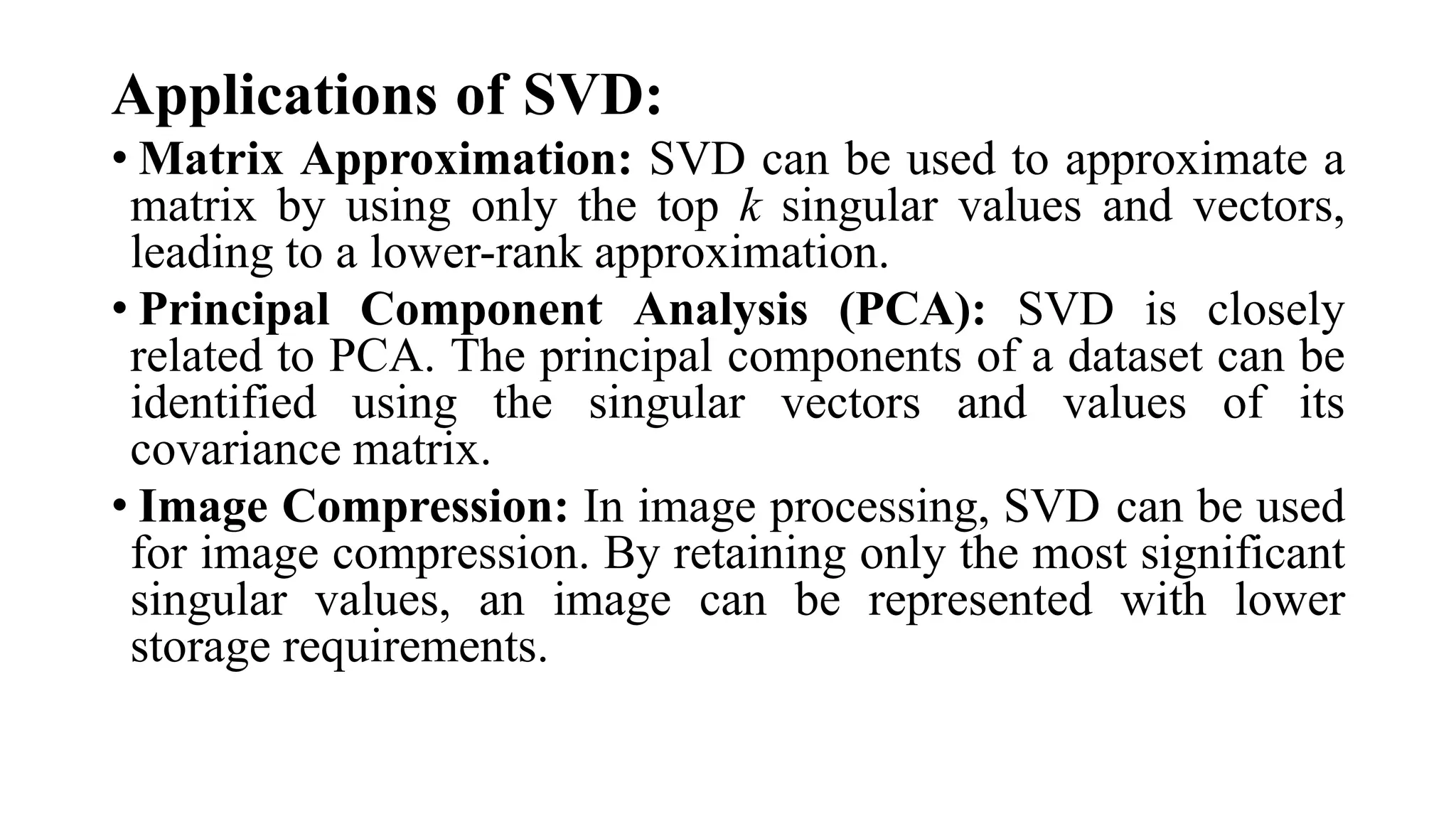
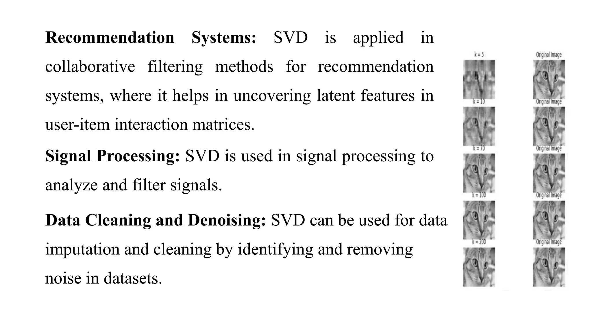
3. Key applications of SVD include matrix approximation, principal component analysis, image compression, recommendation systems, and signal processing.


![R basics for MBA Students[1].pptx](https://cdn.slidesharecdn.com/ss_thumbnails/rbasicsformbastudents1-240213044033-aee3b8d3-thumbnail.jpg?width=640&height=640&fit=bounds)


![Module_-_3_Product_Mgt_&_Pricing[1].pptx](https://cdn.slidesharecdn.com/ss_thumbnails/module-3productmgtpricing1-240418034836-e464c428-thumbnail.jpg?width=640&height=640&fit=bounds)


