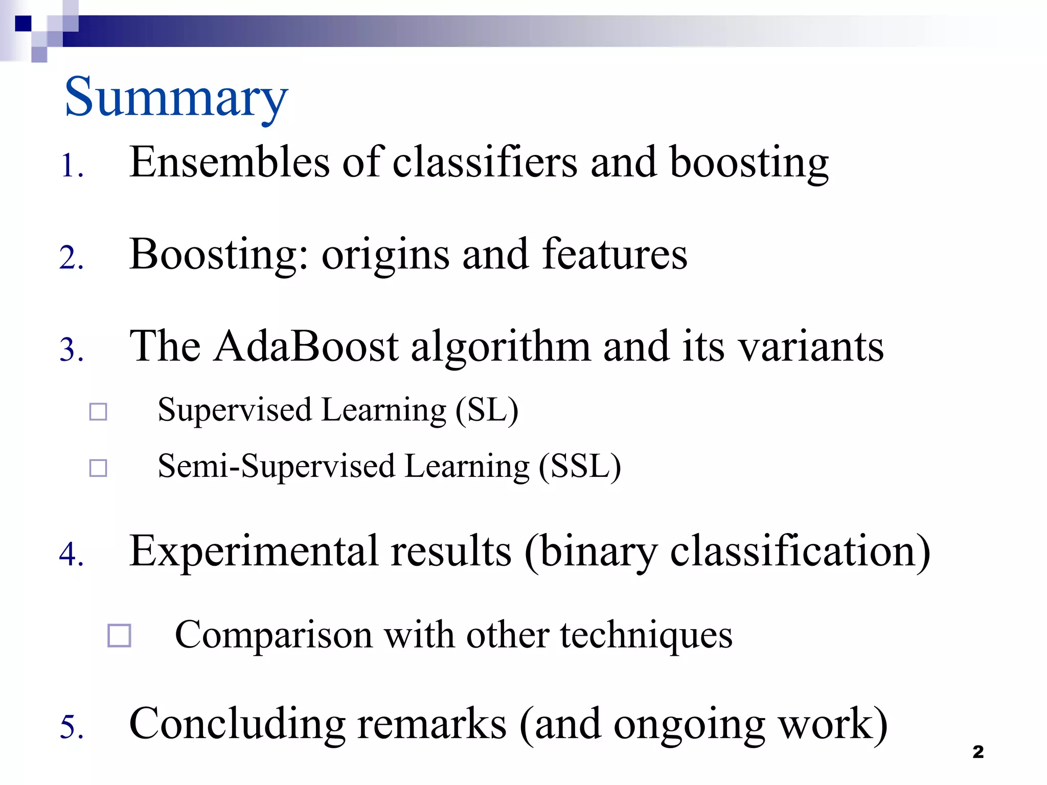
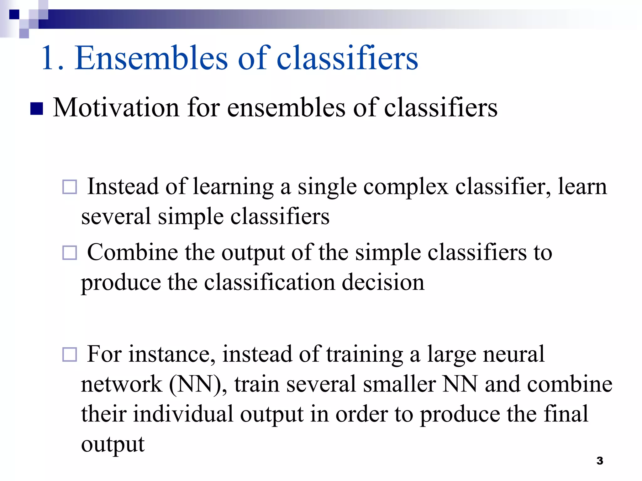
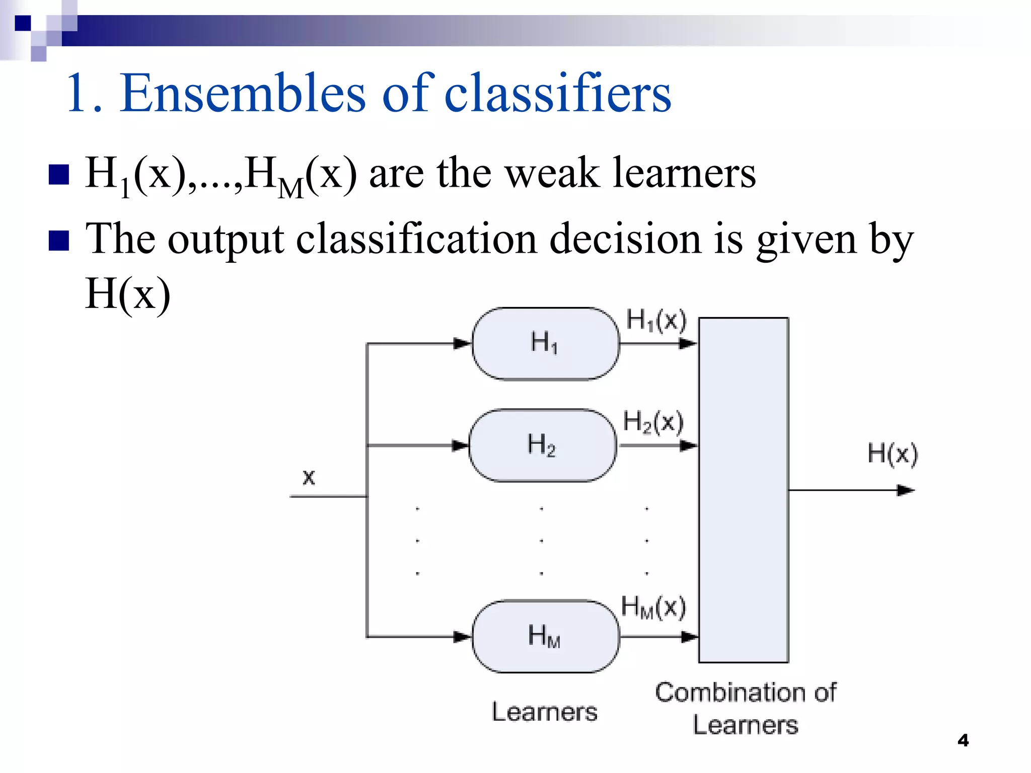
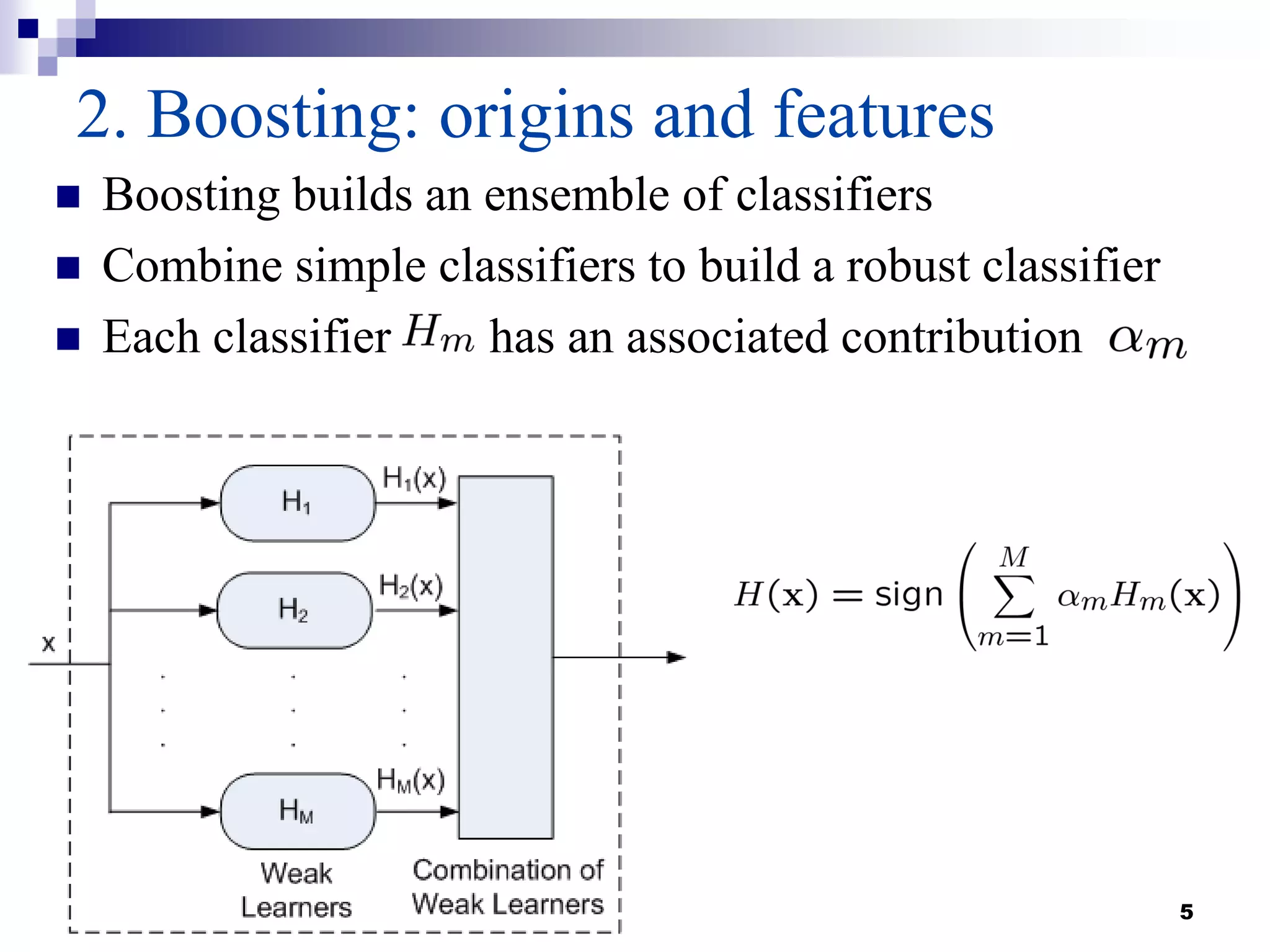
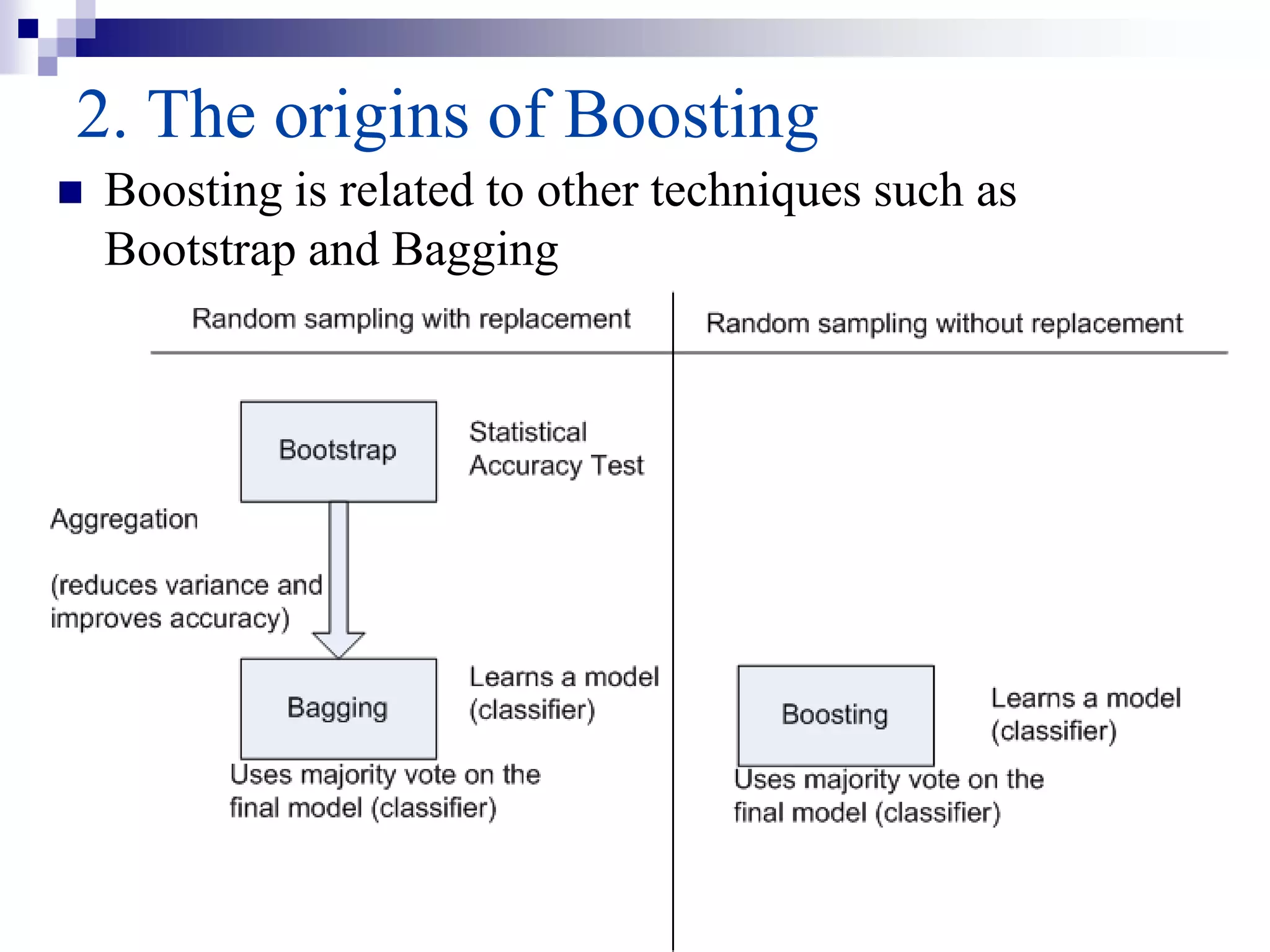
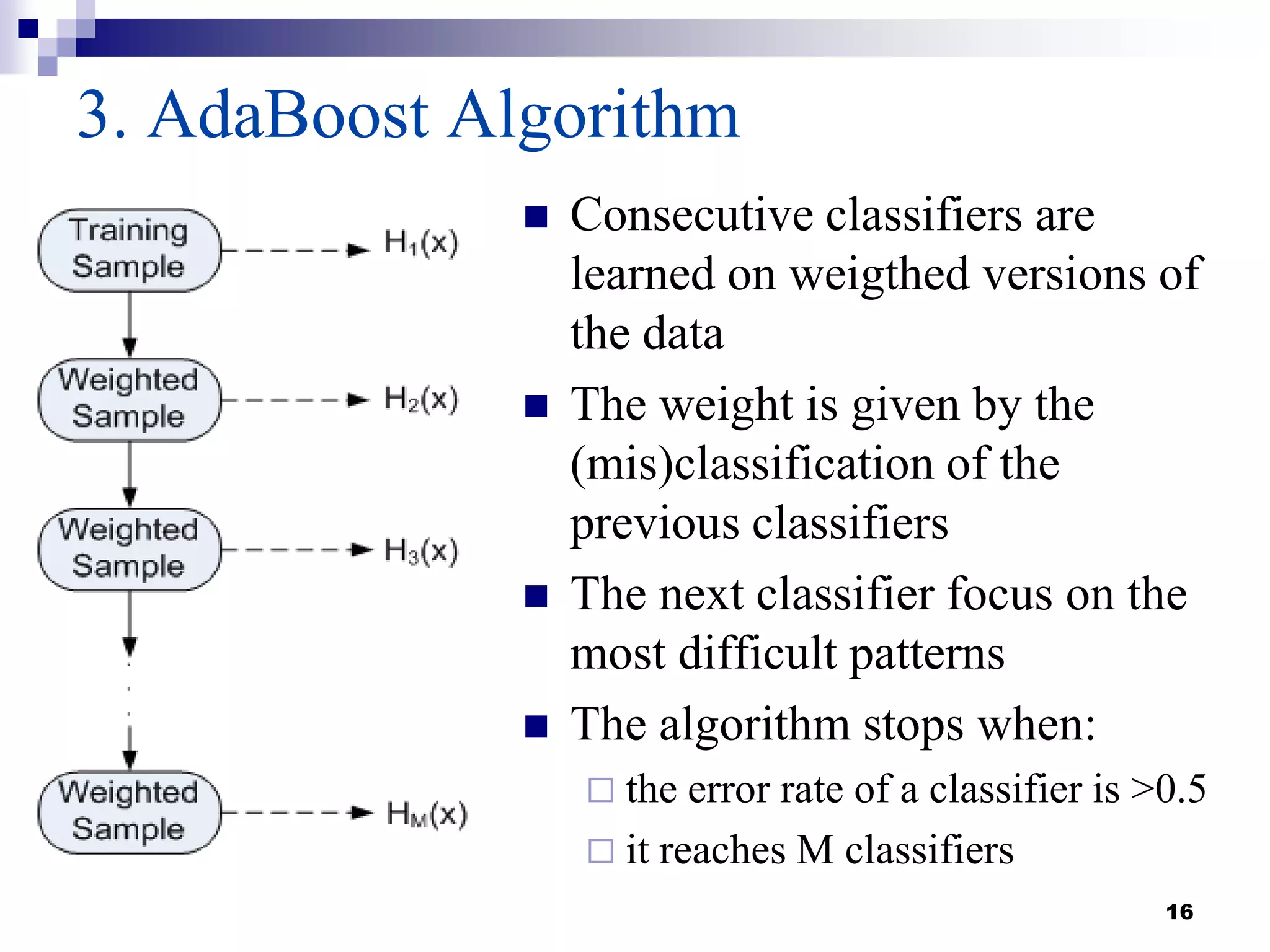
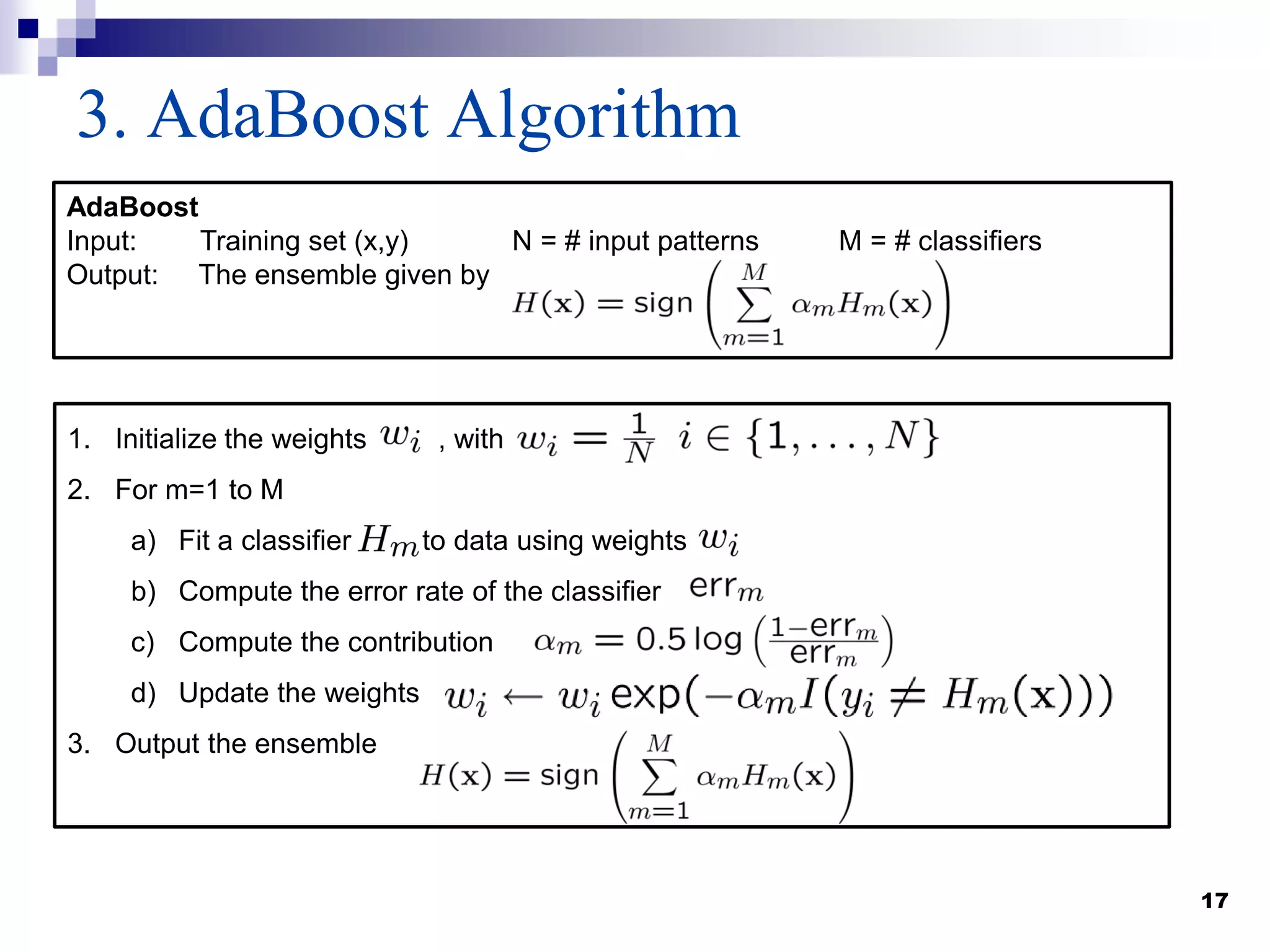
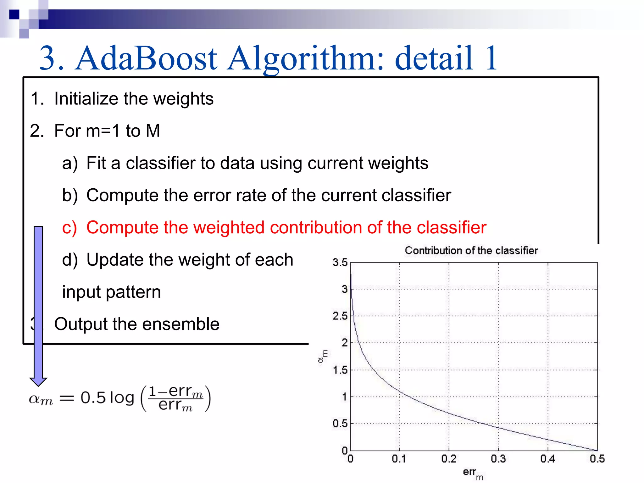
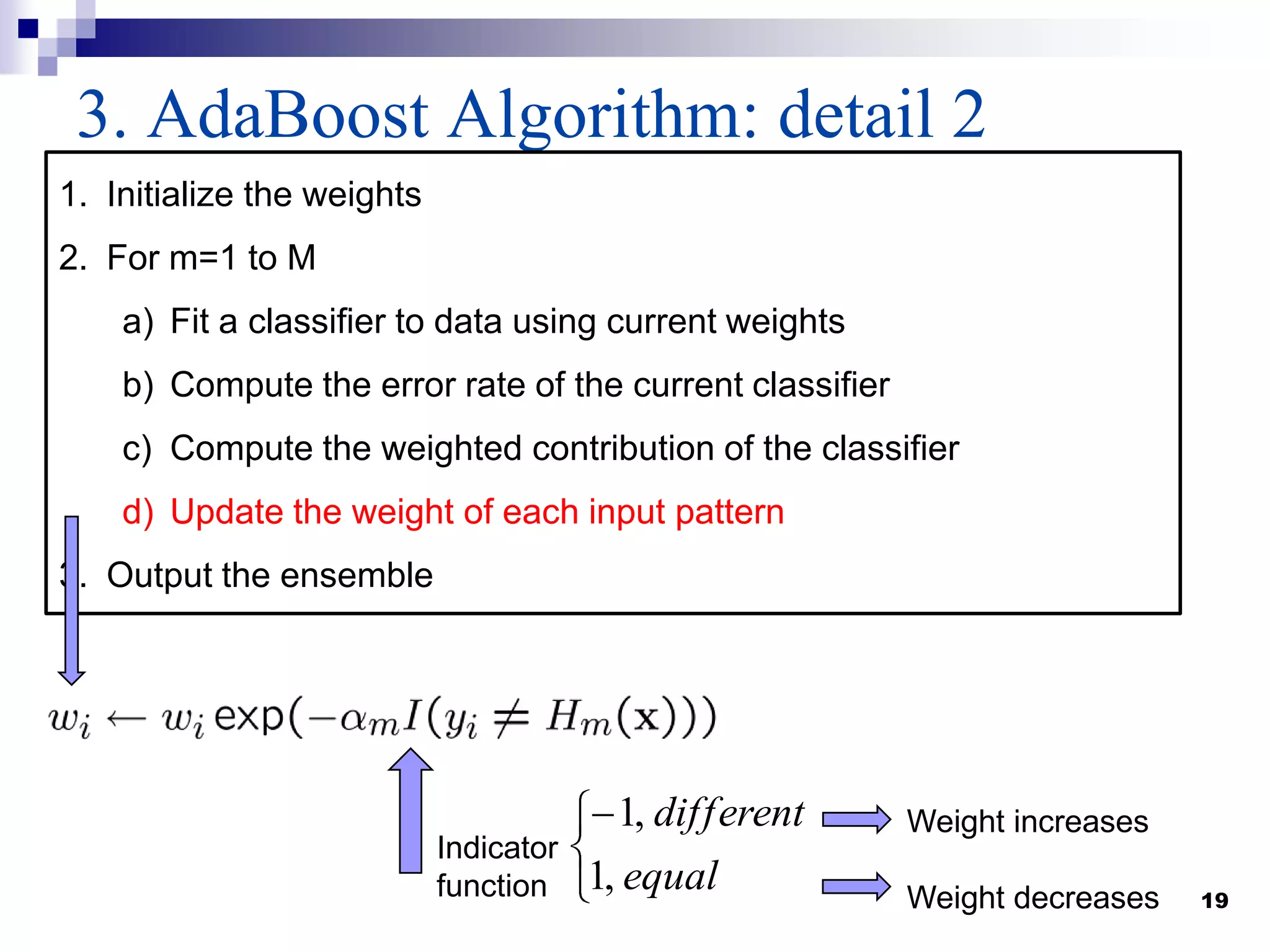
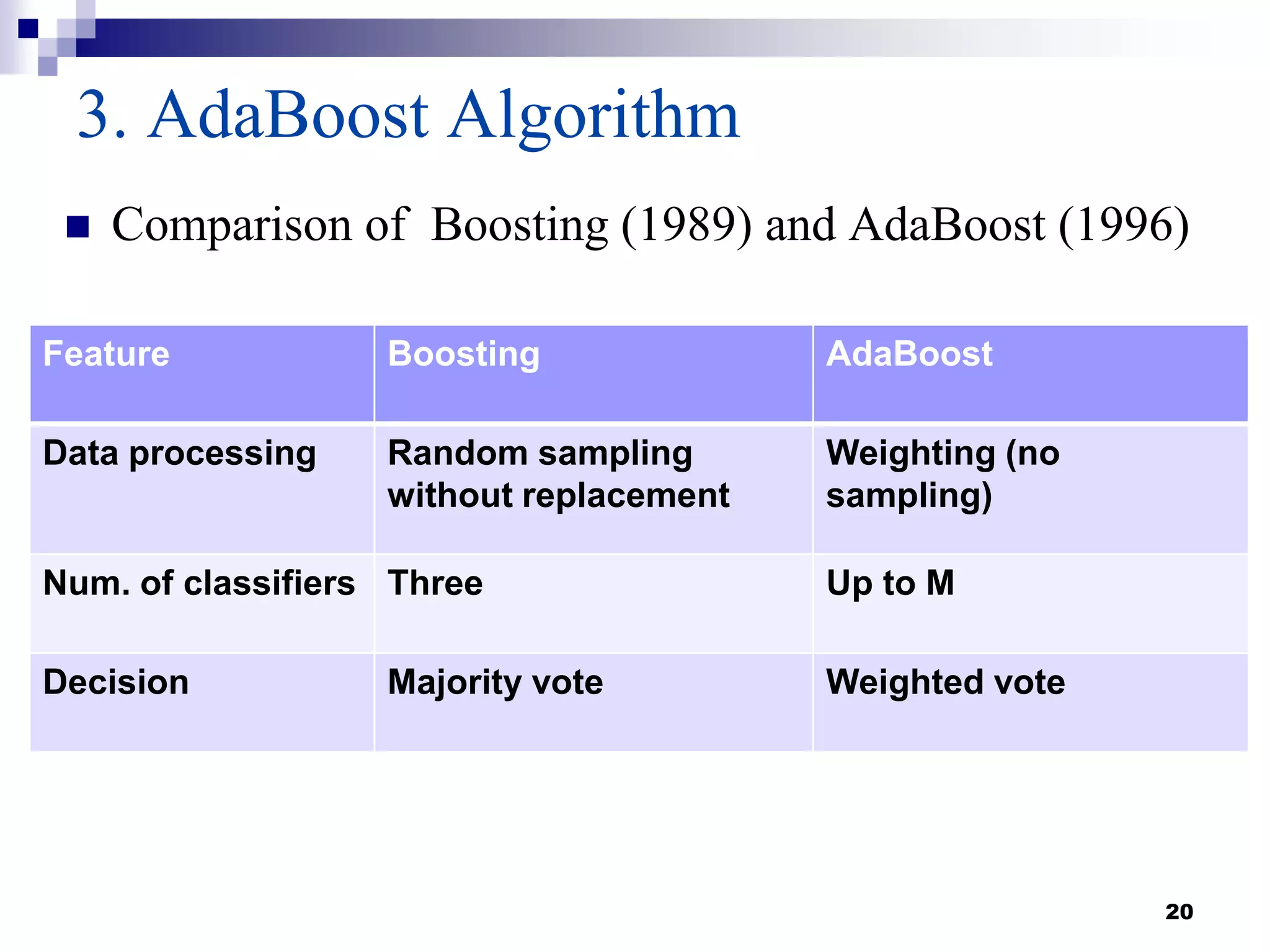
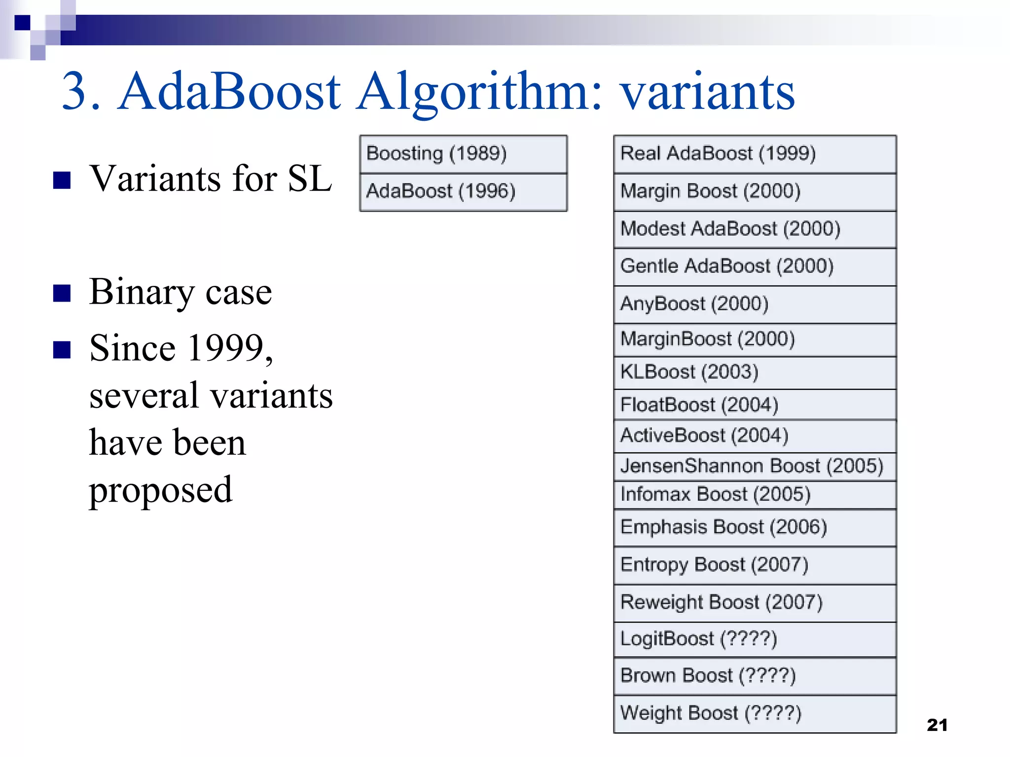
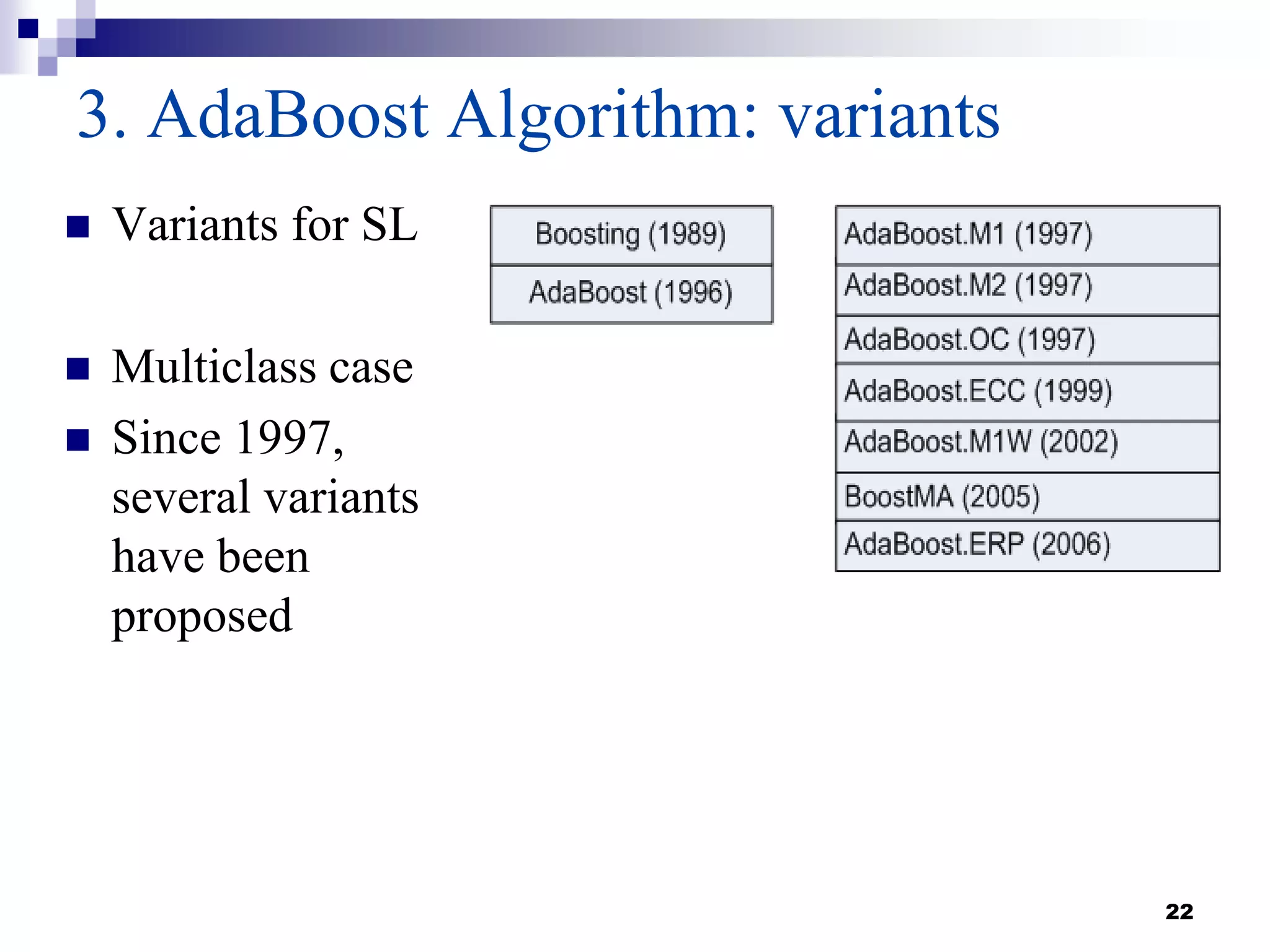
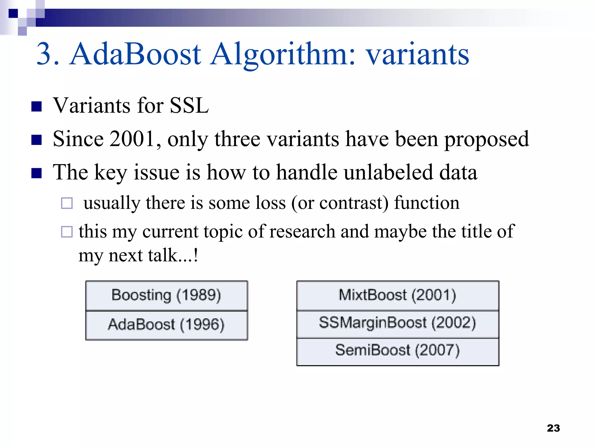
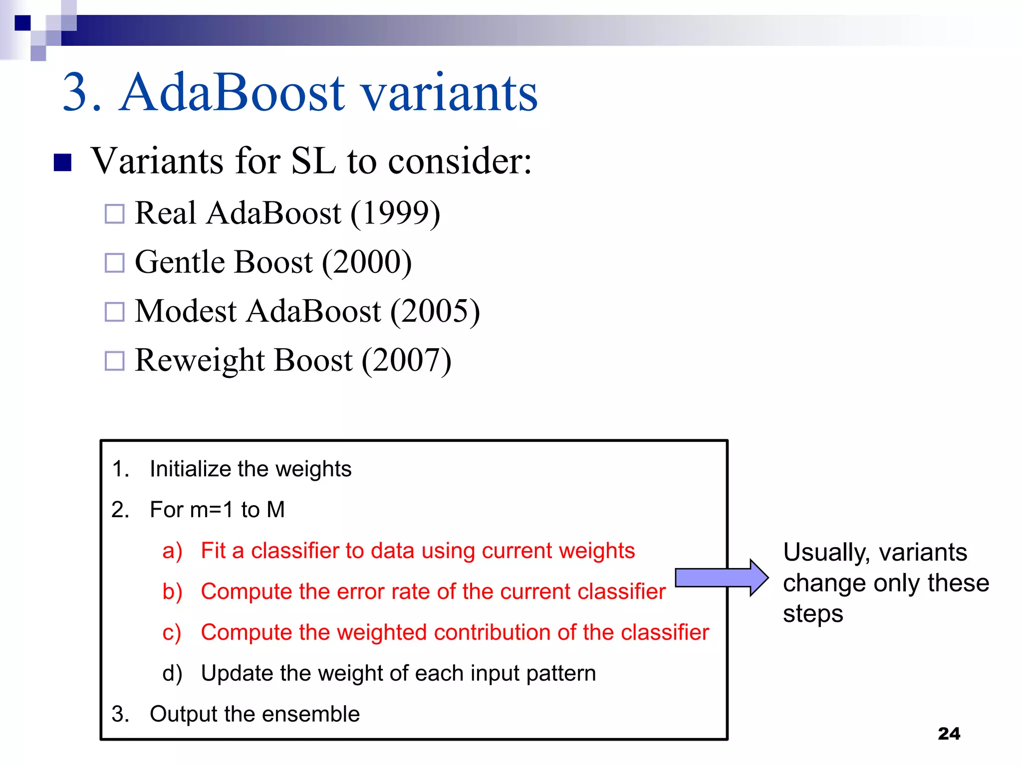
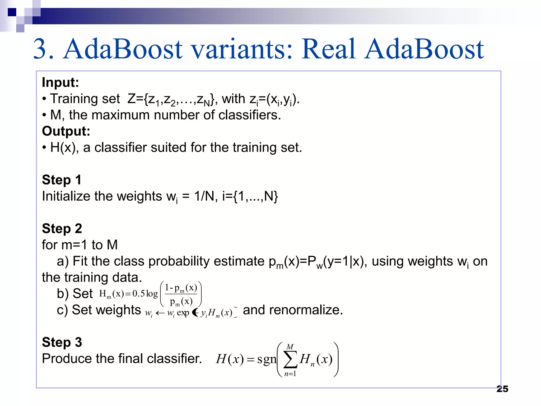
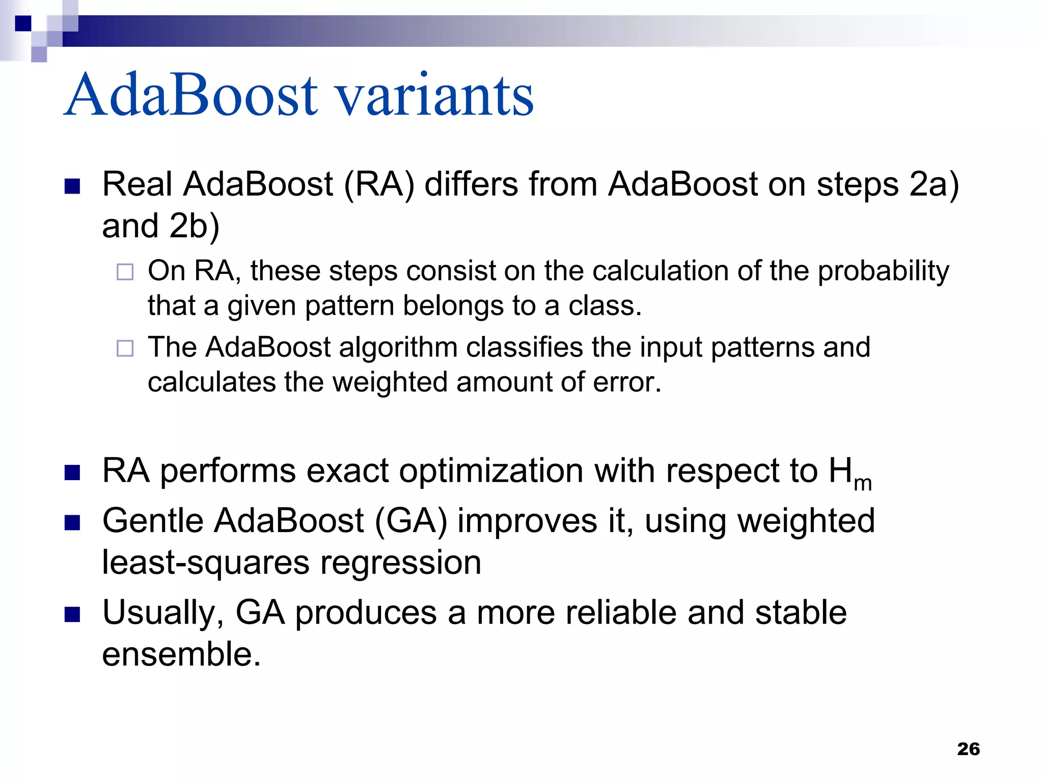
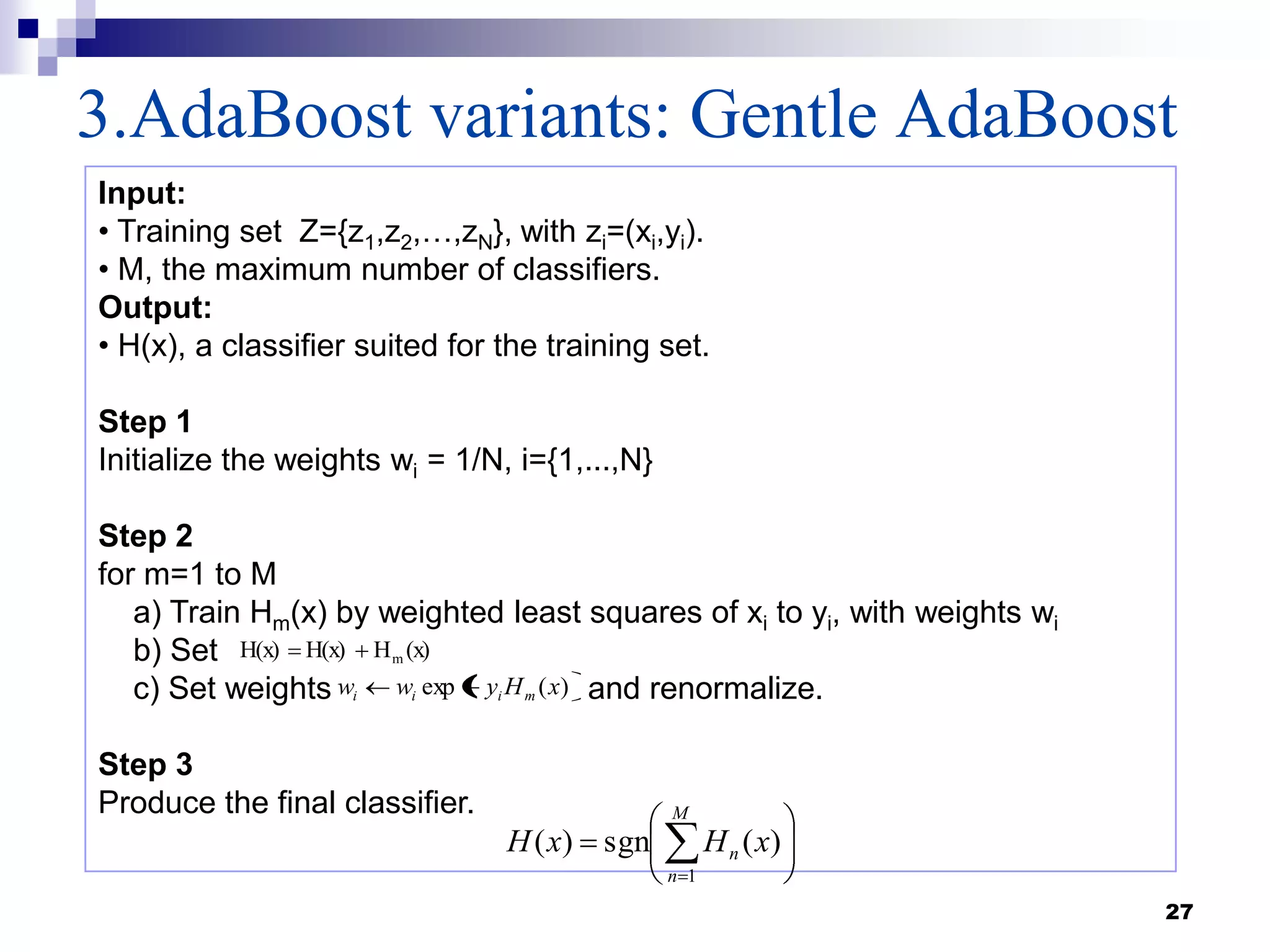
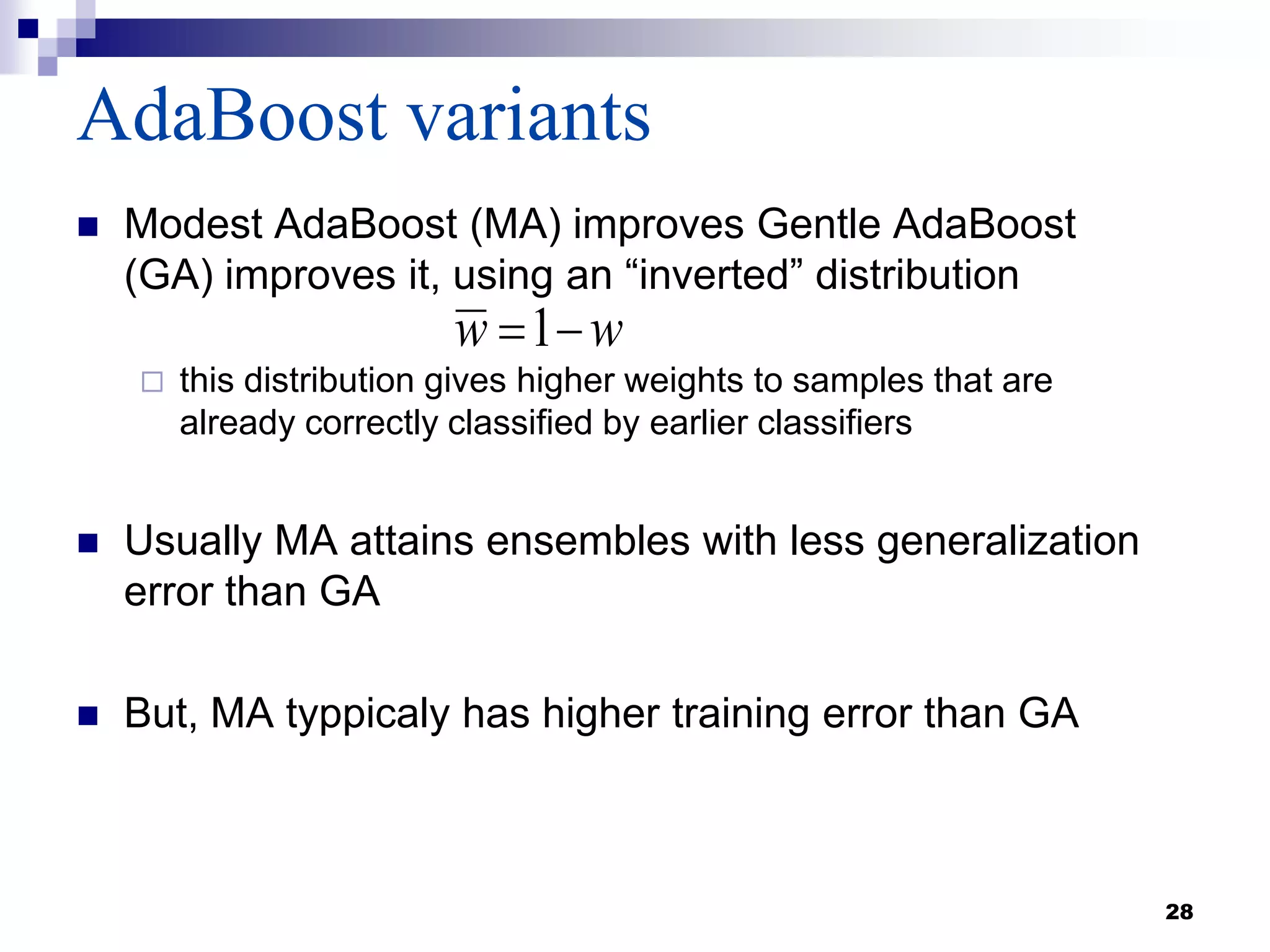
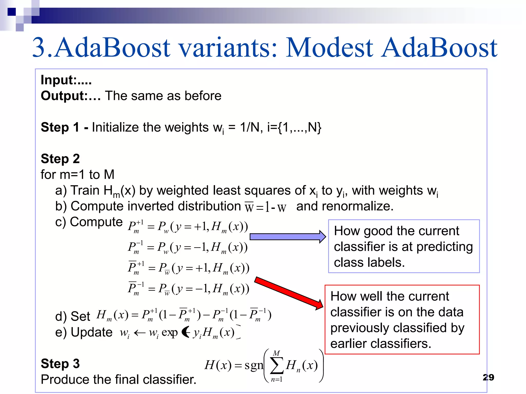
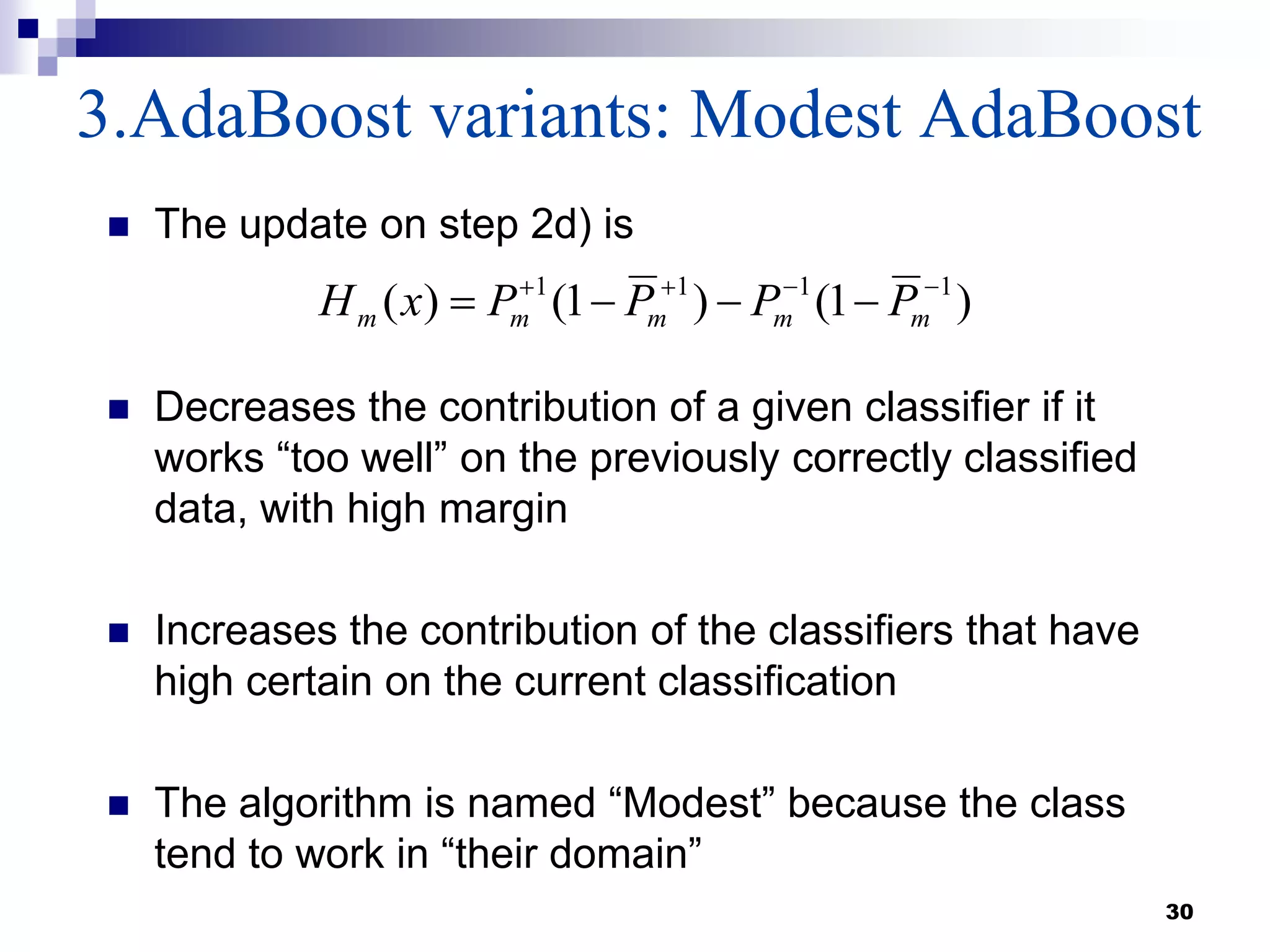
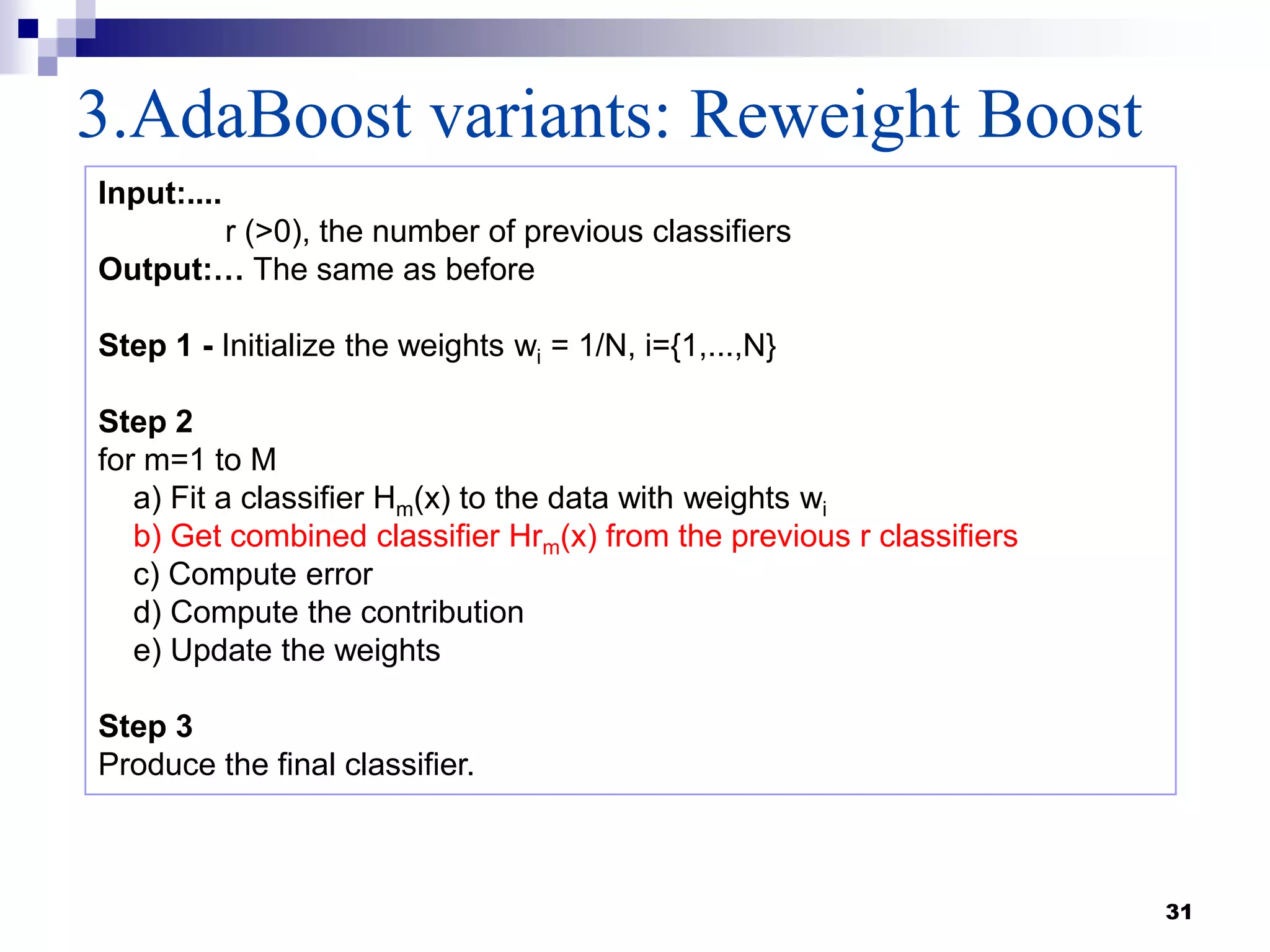
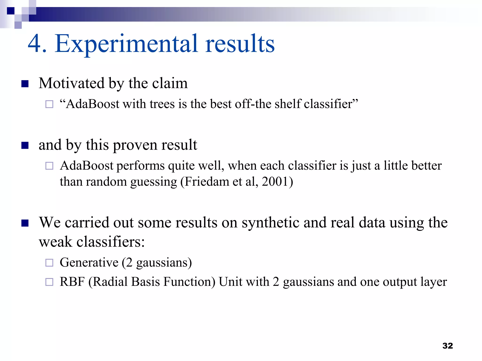
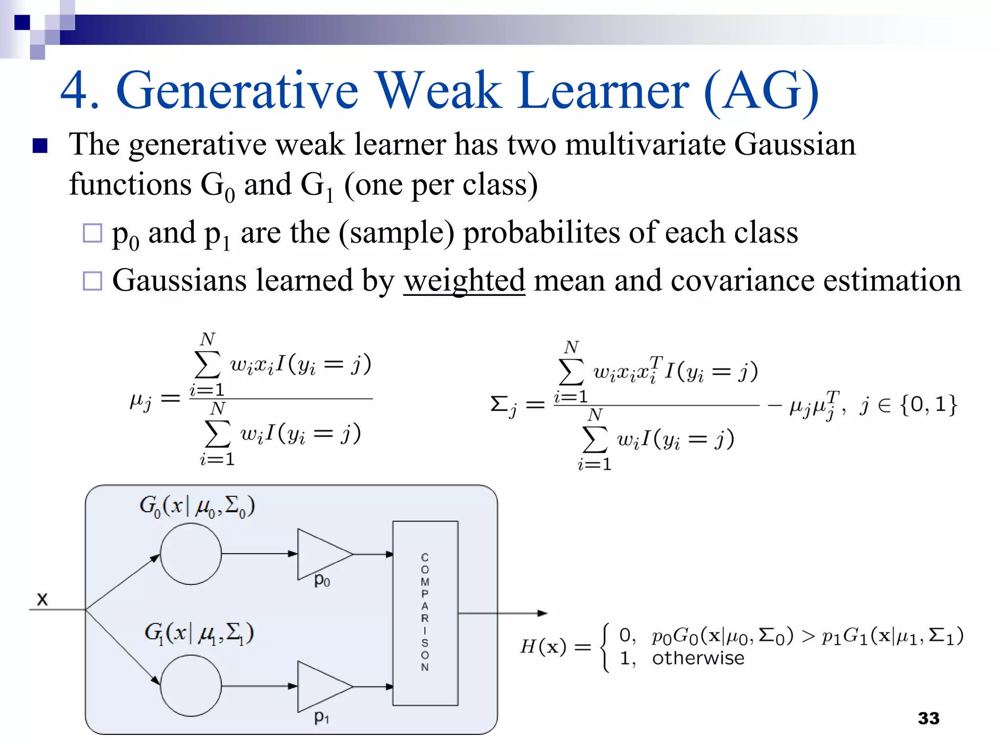
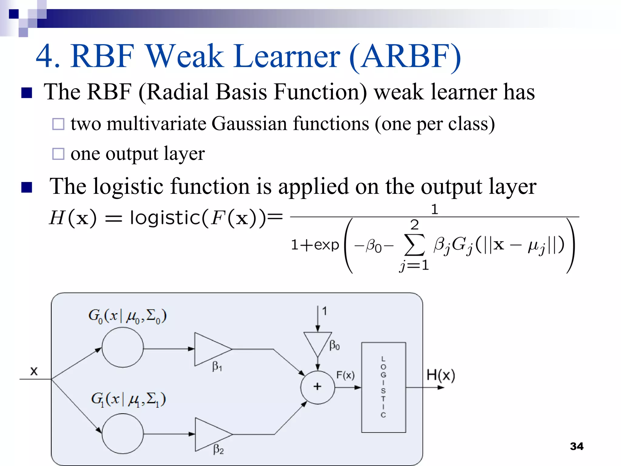
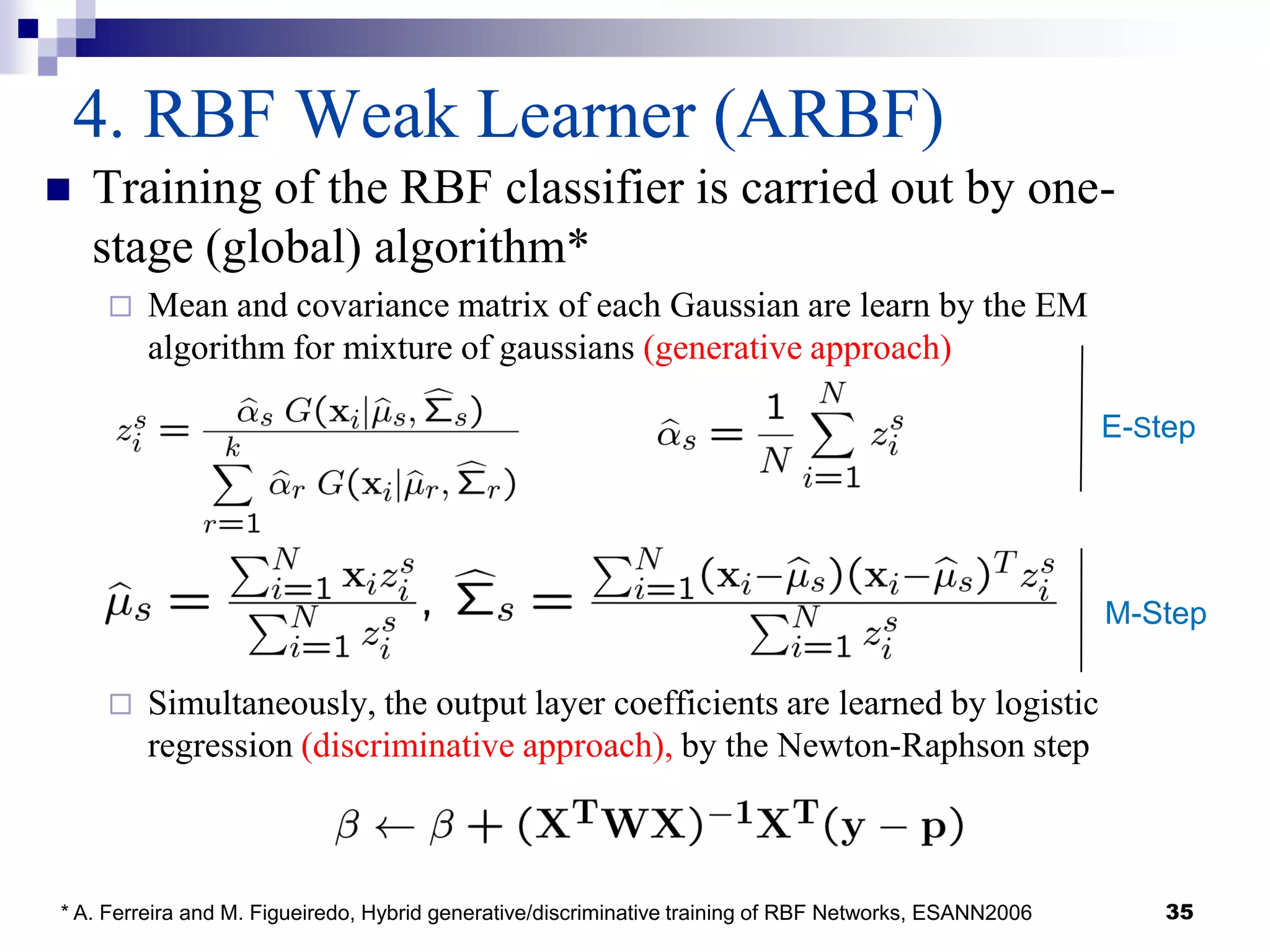
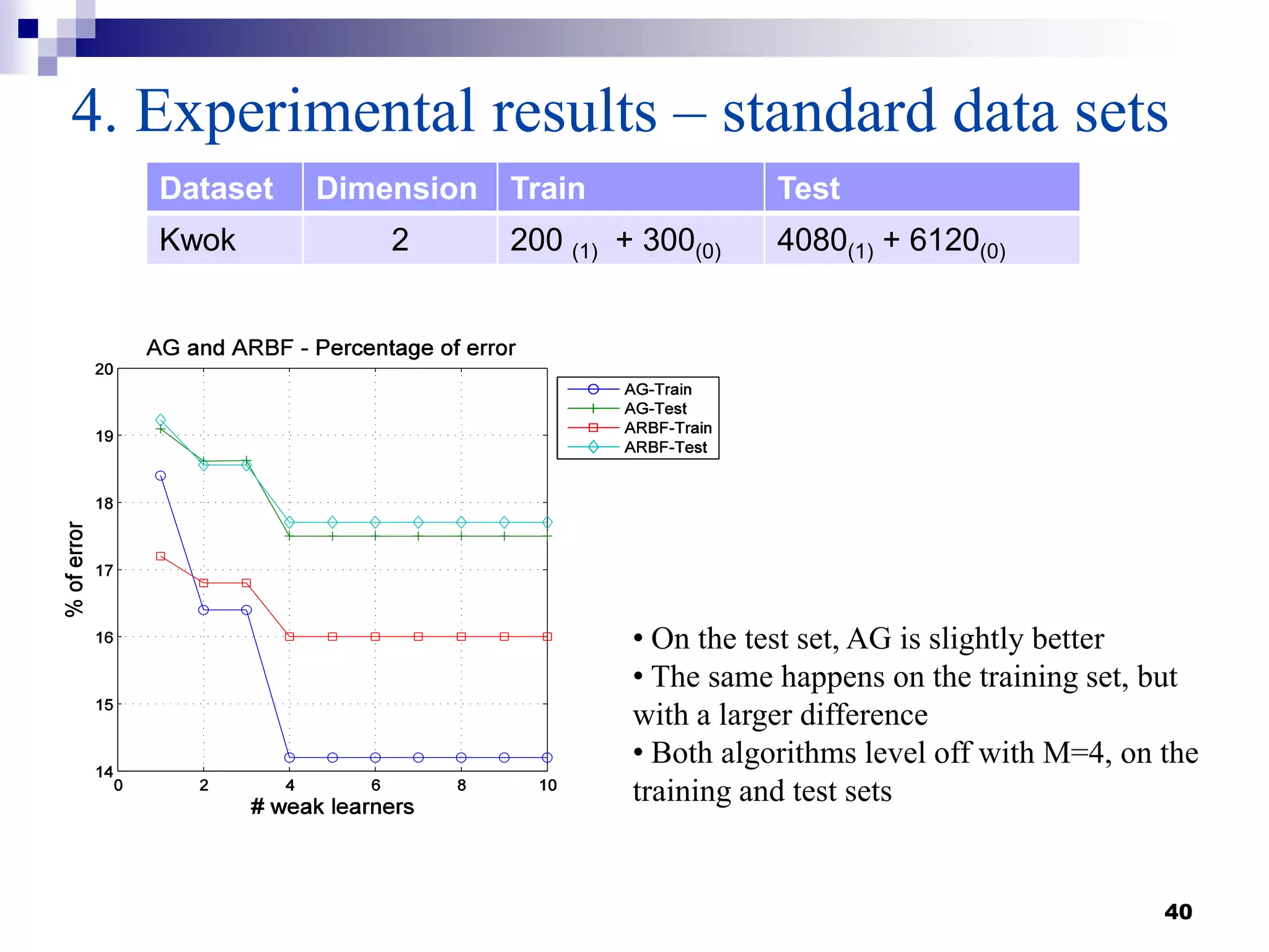
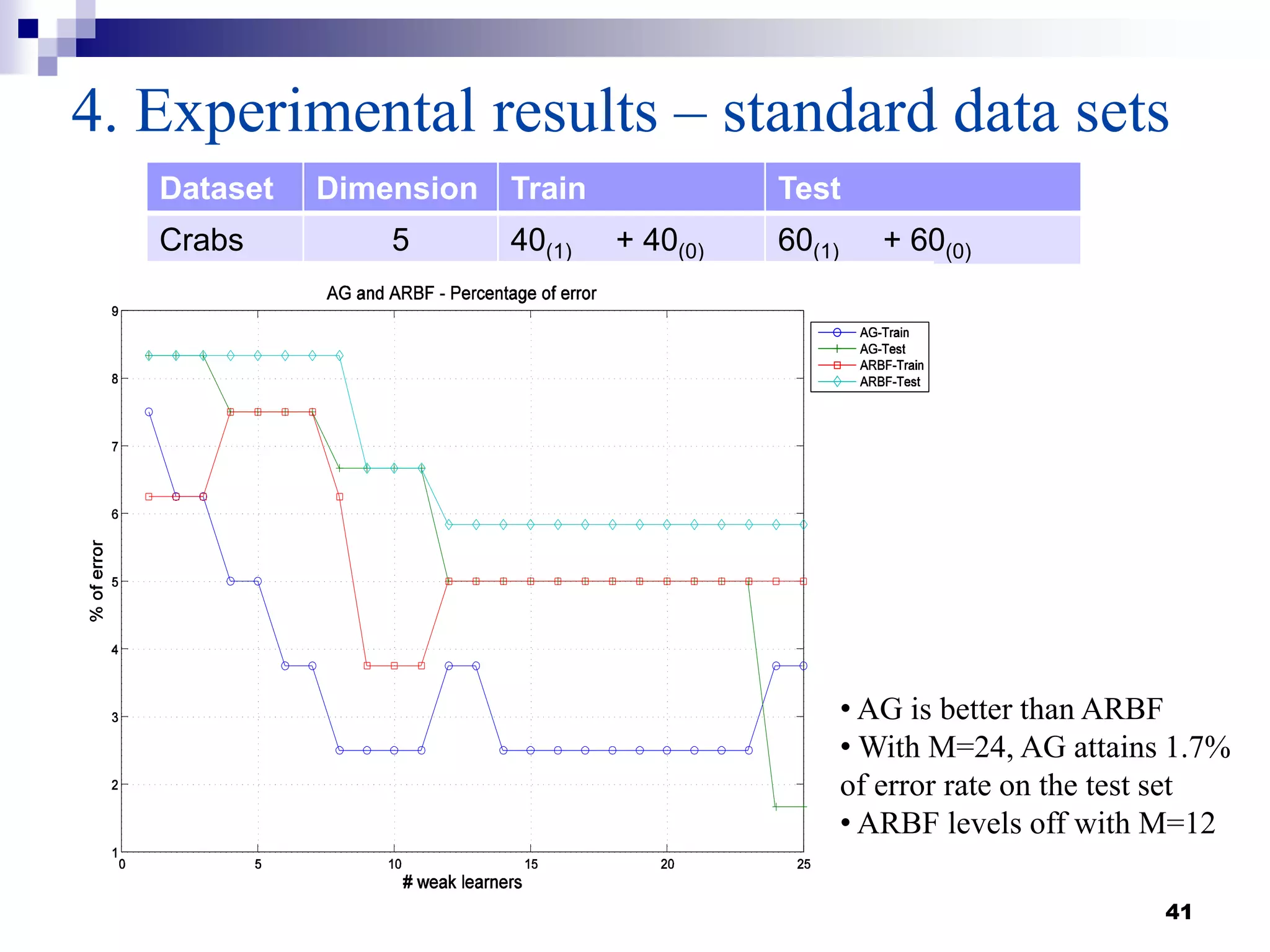
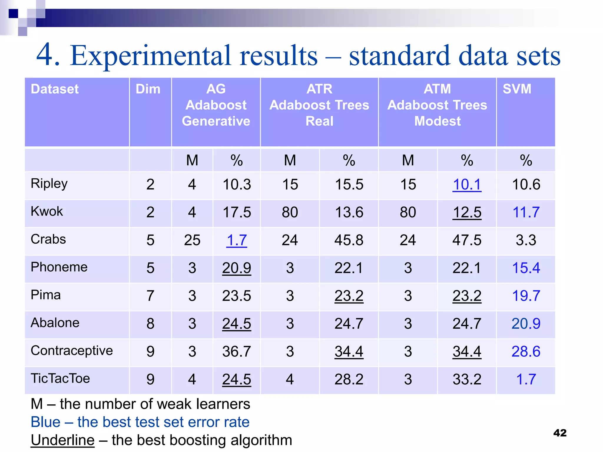
This document summarizes a survey on boosting algorithms for supervised learning. It begins with an introduction to ensembles of classifiers and boosting, describing how boosting builds ensembles by combining simple classifiers with associated contributions. The AdaBoost algorithm and its variants are then explained in detail. Experimental results on synthetic and standard datasets are presented, comparing boosting with generative and RBF weak learners. The results show that boosting algorithms can achieve low error rates, with AdaBoost performing well when weak learners are only slightly better than random.

1. 1
A Survey on
Boosting Algorithms for
Supervised Learning
Artur Ferreira
supervisor Prof. Mário Figueiredo
26 November 2007

2. 2
Summary
1. Ensembles of classifiers and boosting
2. Boosting: origins and features
3. The AdaBoost algorithm and its variants
 Supervised Learning (SL)
 Semi-Supervised Learning (SSL)
4. Experimental results (binary classification)
 Comparison with other techniques
5. Concluding remarks (and ongoing work)

3. 3
1. Ensembles of classifiers
 Motivation for ensembles of classifiers
 Instead of learning a single complex classifier, learn
several simple classifiers
 Combine the output of the simple classifiers to
produce the classification decision
 For instance, instead of training a large neural
network (NN), train several smaller NN and combine
their individual output in order to produce the final
output

4. 4
1. Ensembles of classifiers
 H1(x),...,HM(x) are the weak learners
 The output classification decision is given by
H(x)

5. 5
2. Boosting: origins and features
 Boosting builds an ensemble of classifiers
 Combine simple classifiers to build a robust classifier
 Each classifier has an associated contribution

6. 6
2. The origins of Boosting
 Boosting is related to other techniques such as
Bootstrap and Bagging

7. 7
2. Bootstrap: features
 General purpose sample-based statistical method
 Assesses the statistical accuracy of some estimate S(Z), over a
training set Z={z1, z2,…, zN}, with zi=(xi,yi)
 Draws randomly with replacement from a set of data points,
 Uses B versions of the training set
 To check the accuracy, the measure is applied over the B
sampled versions of the training set

8. 8
2. Bootstrap: graphical idea

9. 9
2. Bootstrap: algorithm
Input:
• Training set Z={z1,z2,…,zN}, with zi=(xi,yi).
• B, number of sampled versions of the training set.
Output:
• S(Z), statistical estimate and its accuracy.
Step 1
for n=1 to B
a) Draw, with replacement, L < N samples from the training set Z,
obtaining the nth sample Z*n.
b) For each sample Z*n, estimate a statistic S (Z*n).
end
Step 2
Produce the bootstrap estimate S(Z), using S (Z*n) with n={1,…,B}.
Step 3
Compute the accuracy of the estimate, using the variance or some other
criterion.

10. 10
2. Bagging: features
 Proposed by Breiman, 1996
 Consists of Bootstrap aggregation
 Training set Z={z1, z2,…, zN}, with zi=(xi,yi) for
which we intend to fit a model f(x)
 Obtain a prediction of f(x) at input x
 For each bootstrap sample b we fit our model,
giving a prediction fb(x).
 The Bagging estimate is the average of the
individual estimates

11. 11
2. Bagging: algorithm (classification)
Input:
• Training set Z={z1,z2,…,zN}, with zi=(xi,yi).
• B, number of sampled versions of the training set.
Output:
• H(x), a classifier suited for the training set.
Step 1
for n=1 to B
a) Draw, with replacement, L < N samples from the training set Z,
obtaining the nth sample Z*n.
b) For each sample Z*n, learn classifier Hn.
end
Step 2
Produce the final classifier as a vote of Hn with n={1,…,B}.
B
n
n xHxH
1
)(sgn)(

12. 12
2. Boosting: features
 Freund and Schapire, 1989
 Similar to Bagging, in the sense that uses
several versions of the training set
 Uses 3 subsets of the training set
 Differs from Bagging, in the sense that does not
allow replacement
 The final classification is done my a majority
vote (3 classifiers)

13. 13
2. Boosting: algorithm (classification)
Input:
• Training set Z={z1,z2,…,zN}, with zi=(xi,yi).
Output:
• H(x), a classifier suited for the training set.
Step 1 - Draw, without replacement, L < N samples from the training set Z,
obtaining Z*1; train weak learner H1 on Z*1
Step 2 - Select L2 < N samples from Z with half of the samples
misclassified by H1 to obtain Z*2; train weak learner H2 on it.
Step 3 - Select all samples from Z that H1 and H2 disagree on; train weak
learner H3, using these samples.
Step 4 - Produce the final classifier as a vote of the three weak learners
3
1
)(sgn)(
n
n xHxH

14. 14
2. Boosting: graphical idea

15. 15
3. AdaBoost Algorithm
 Adaptive Boosting
 By Freund and Schapire, 1996
 Instead of sample, reweight the
data
 Consecutive classifiers are
learned on weigthed versions
of the data
 The entire training set is
considered in order to learn
each classifier

16. 16
3. AdaBoost Algorithm
 Consecutive classifiers are
learned on weigthed versions of
the data
 The weight is given by the
(mis)classification of the
previous classifiers
 The next classifier focus on the
most difficult patterns
 The algorithm stops when:
 the error rate of a classifier is >0.5
 it reaches M classifiers

17. 17
3. AdaBoost Algorithm
1. Initialize the weights , with
2. For m=1 to M
a) Fit a classifier to data using weights
b) Compute the error rate of the classifier
c) Compute the contribution
d) Update the weights
3. Output the ensemble
AdaBoost
Input: Training set (x,y) N = # input patterns M = # classifiers
Output: The ensemble given by

18. 18
3. AdaBoost Algorithm: detail 1
1. Initialize the weights
2. For m=1 to M
a) Fit a classifier to data using current weights
b) Compute the error rate of the current classifier
c) Compute the weighted contribution of the classifier
d) Update the weight of each
input pattern
3. Output the ensemble

19. 19
3. AdaBoost Algorithm: detail 2
1. Initialize the weights
2. For m=1 to M
a) Fit a classifier to data using current weights
b) Compute the error rate of the current classifier
c) Compute the weighted contribution of the classifier
d) Update the weight of each input pattern
3. Output the ensemble
Indicator
function equal
different
,1
,1 Weight increases
Weight decreases

20. 20
3. AdaBoost Algorithm
 Comparison of Boosting (1989) and AdaBoost (1996)
Feature Boosting AdaBoost
Data processing Random sampling
without replacement
Weighting (no
sampling)
Num. of classifiers Three Up to M
Decision Majority vote Weighted vote

21. 21
3. AdaBoost Algorithm: variants
 Variants for SL
 Binary case
 Since 1999,
several variants
have been
proposed

22. 22
3. AdaBoost Algorithm: variants
 Variants for SL
 Multiclass case
 Since 1997,
several variants
have been
proposed

23. 23
3. AdaBoost Algorithm: variants
 Variants for SSL
 Since 2001, only three variants have been proposed
 The key issue is how to handle unlabeled data
 usually there is some loss (or contrast) function
 this my current topic of research and maybe the title of
my next talk...!

24. 24
3. AdaBoost variants
 Variants for SL to consider:
 Real AdaBoost (1999)
 Gentle Boost (2000)
 Modest AdaBoost (2005)
 Reweight Boost (2007)
1. Initialize the weights
2. For m=1 to M
a) Fit a classifier to data using current weights
b) Compute the error rate of the current classifier
c) Compute the weighted contribution of the classifier
d) Update the weight of each input pattern
3. Output the ensemble
Usually, variants
change only these
steps

25. 3. AdaBoost variants: Real AdaBoost
25
Input:
• Training set Z={z1,z2,…,zN}, with zi=(xi,yi).
• M, the maximum number of classifiers.
Output:
• H(x), a classifier suited for the training set.
Step 1
Initialize the weights wi = 1/N, i={1,...,N}
Step 2
for m=1 to M
a) Fit the class probability estimate pm(x)=Pw(y=1|x), using weights wi on
the training data.
b) Set
c) Set weights and renormalize.
Step 3
Produce the final classifier.
(x)p
(x)p-1
log0.5(x)H
m
m
m
)(exp xHyww miii
M
n
n xHxH
1
)(sgn)(

26. AdaBoost variants
 Real AdaBoost (RA) differs from AdaBoost on steps 2a)
and 2b)
 On RA, these steps consist on the calculation of the probability
that a given pattern belongs to a class.
 The AdaBoost algorithm classifies the input patterns and
calculates the weighted amount of error.
 RA performs exact optimization with respect to Hm
 Gentle AdaBoost (GA) improves it, using weighted
least-squares regression
 Usually, GA produces a more reliable and stable
ensemble.
26

27. 3.AdaBoost variants: Gentle AdaBoost
27
Input:
• Training set Z={z1,z2,…,zN}, with zi=(xi,yi).
• M, the maximum number of classifiers.
Output:
• H(x), a classifier suited for the training set.
Step 1
Initialize the weights wi = 1/N, i={1,...,N}
Step 2
for m=1 to M
a) Train Hm(x) by weighted least squares of xi to yi, with weights wi
b) Set
c) Set weights and renormalize.
Step 3
Produce the final classifier.
(x)HH(x)H(x) m
)(exp xHyww miii
M
n
n xHxH
1
)(sgn)(

28. AdaBoost variants
 Modest AdaBoost (MA) improves Gentle AdaBoost
(GA) improves it, using an “inverted” distribution
 this distribution gives higher weights to samples that are
already correctly classified by earlier classifiers
 Usually MA attains ensembles with less generalization
error than GA
 But, MA typpicaly has higher training error than GA
28
ww 1

29. 3.AdaBoost variants: Modest AdaBoost
29
Input:....
Output:… The same as before
Step 1 - Initialize the weights wi = 1/N, i={1,...,N}
Step 2
for m=1 to M
a) Train Hm(x) by weighted least squares of xi to yi, with weights wi
b) Compute inverted distribution and renormalize.
c) Compute
d) Set
e) Update
Step 3
Produce the final classifier.
w-1w
)(exp xHyww miii
M
n
n xHxH
1
)(sgn)(
))(,1(
))(,1(
))(,1(
))(,1(
1
1
1
1
xHyPP
xHyPP
xHyPP
xHyPP
mwm
mwm
mwm
mwm
)1()1()( 1111
mmmmm PPPPxH
How good the current
classifier is at predicting
class labels.
How well the current
classifier is on the data
previously classified by
earlier classifiers.

30. 3.AdaBoost variants: Modest AdaBoost
30
 The update on step 2d) is
 Decreases the contribution of a given classifier if it
works “too well” on the previously correctly classified
data, with high margin
 Increases the contribution of the classifiers that have
high certain on the current classification
 The algorithm is named “Modest” because the class
tend to work in “their domain”
)1()1()( 1111
mmmmm PPPPxH

31. 3.AdaBoost variants: Reweight Boost
31
Input:....
r (>0), the number of previous classifiers
Output:… The same as before
Step 1 - Initialize the weights wi = 1/N, i={1,...,N}
Step 2
for m=1 to M
a) Fit a classifier Hm(x) to the data with weights wi
b) Get combined classifier Hrm(x) from the previous r classifiers
c) Compute error
d) Compute the contribution
e) Update the weights
Step 3
Produce the final classifier.

32. 32
4. Experimental results
 Motivated by the claim
 “AdaBoost with trees is the best off-the shelf classifier”
 and by this proven result
 AdaBoost performs quite well, when each classifier is just a little better
than random guessing (Friedam et al, 2001)
 We carried out some results on synthetic and real data using the
weak classifiers:
 Generative (2 gaussians)
 RBF (Radial Basis Function) Unit with 2 gaussians and one output layer

33. 33
4. Generative Weak Learner (AG)
 The generative weak learner has two multivariate Gaussian
functions G0 and G1 (one per class)
 p0 and p1 are the (sample) probabilites of each class
 Gaussians learned by weighted mean and covariance estimation

34. 34
4. RBF Weak Learner (ARBF)
 The RBF (Radial Basis Function) weak learner has
 two multivariate Gaussian functions (one per class)
 one output layer
 The logistic function is applied on the output layer

35. 35
4. RBF Weak Learner (ARBF)
 Training of the RBF classifier is carried out by one-
stage (global) algorithm*
 Mean and covariance matrix of each Gaussian are learn by the EM
algorithm for mixture of gaussians (generative approach)
 Simultaneously, the output layer coefficients are learned by logistic
regression (discriminative approach), by the Newton-Raphson step
* A. Ferreira and M. Figueiredo, Hybrid generative/discriminative training of RBF Networks, ESANN2006
E-Step
M-Step

36. 36
4. Experimental results – synthetic 1
 Synthetic 1 dataset: two-dimensional; 100 train patterns (50 +
50); 400 test patterns (200 + 200)
 Using up to M=10 classifiers
 Test set error rate: AG (M=10) 6.5% ARBF (M=3) 1%
AG ARBF

37. 37
4. Experimental results – synthetic 1
 Synthetic 1 dataset: two-dimensional; 100 train patterns (50 +
50); 400 test patterns (200 + 200)
 Using up to M=10 classifiers
 Training and test set error rate, as a function of M
• ARBF obtains better results, but is
unable to achieve zero errors on the
test set
• For both algorithms, after a given
value of M, there is no decrease on the
error

38. 38
4. Experimental results – synthetic 2
AG ARBF
 Synthetic 2 dataset: two-dimensional; 180 train patterns (90 +
90); 360 test patterns (180 + 180)
 Using up to M=15 classifiers
 Test set error rate: AG (M=15) 0.28% ARBF (M=15) 0.83%

39. 39
4. Experimental results – synthetic 2
 Synthetic 2 dataset: two-dimensional; 180 train patterns (90 +
90); 360 test patterns (180 + 180)
 Using up to M=15 classifiers
 Training and test set error rate, as a function of M
• In this case, AG achieves better results
• Unable to achieve zero errors on the test set
• ARBF levels off with M=6
• For AG we have it with M=12

40. 40
4. Experimental results – standard data sets
Dataset Dimension Train Test
Kwok 2 200 (1) + 300(0) 4080(1) + 6120(0)
• On the test set, AG is slightly better
• The same happens on the training set, but
with a larger difference
• Both algorithms level off with M=4, on the
training and test sets

41. 41
4. Experimental results – standard data sets
Dataset Dimension Train Test
Crabs 5 40(1) + 40(0) 60(1) + 60(0)
• AG is better than ARBF
• With M=24, AG attains 1.7%
of error rate on the test set
• ARBF levels off with M=12

42. 42
4. Experimental results – standard data sets
Dataset Dim AG
Adaboost
Generative
ATR
Adaboost Trees
Real
ATM
Adaboost Trees
Modest
SVM
M % M % M % %
Ripley 2 4 10.3 15 15.5 15 10.1 10.6
Kwok 2 4 17.5 80 13.6 80 12.5 11.7
Crabs 5 25 1.7 24 45.8 24 47.5 3.3
Phoneme 5 3 20.9 3 22.1 3 22.1 15.4
Pima 7 3 23.5 3 23.2 3 23.2 19.7
Abalone 8 3 24.5 3 24.7 3 24.7 20.9
Contraceptive 9 3 36.7 3 34.4 3 34.4 28.6
TicTacToe 9 4 24.5 4 28.2 3 33.2 1.7
M – the number of weak learners
Blue – the best test set error rate
Underline – the best boosting algorithm

43. 43
4. Experimental results
Detector AdaBoost Variant Weak Learner
Viola-Jones (2001) Discrete AdaBoost Stub
Float Boost (2004) Float Boost 1D Histograms
KLBoost (2003) KLBoost 1D Histograms
Schneiderman Real AdaBoost One group of n-D
Histograms
 Application to face detection

44. 44
5. Concluding remarks
 Adaptive Boosting is a field of intensive research
 The main focus of research is for SSL
 It seems to be “easy” to accomodate for unlabeled data
 Our tests, on SL, showed that:
 Boosting of generative and RBF classifiers achieve performance close to
boosting of trees, on standard datasets
 Good performance with low training complexity, suited for embedded
systems
 AG and ARBF obtain results close to SVM, using a small number of weak
learners
 Typically, (the simpler) AG attains better results than ARBF
 For high-dimensional datasets (with small training set) may be necessary
to use diagonal covariances

45. 45
5. Concluding remarks: ongoing work
 For SL:
 Establish (one more!) variant of AdaBoost, using the logistic
function
 The logistic function gives us a degree of confidence on the
classification
 For SSL:
 Study and minor modifications of existing boosting
algorithms
 MixtBoost, SSMarginBoost, SemiBoost
 Extend our AdaBoost variant, proposed for SL, to SSL
 using the logistic function properties to accommodate for unlabeled data

46. 46
5. Concluding remarks: ongoing work
 Logistic Function
)exp(1
1
)(
a
al