Downloaded 143 times


![Supervised learning
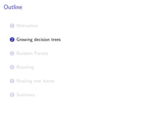
• Data comes as a finite learning set L = (X, y) where
Input samples are given as an array of shape (n samples,
n features)
E.g., feature values for wine physicochemical properties:
# fixed acidity, volatile acidity, ...
X = [[ 7.4 0. ... 0.56 9.4 0. ]
[ 7.8 0. ... 0.68 9.8 0. ]
...
[ 7.8 0.04 ... 0.65 9.8 0. ]]
Output values are given as an array of shape (n samples,)
E.g., wine taste preferences (from 0 to 10):
y = [5 5 5 ... 6 7 6]
• The goal is to build an estimator ϕL : X → Y minimizing
Err(ϕL) = EX,Y {L(Y , ϕL.predict(X))}.
5 / 26](https://image.slidesharecdn.com/slides-150408072332-conversion-gate01/85/Tree-models-with-Scikit-Learn-Great-models-with-little-assumptions-6-320.jpg)
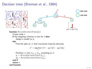


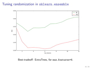
![Tuning randomization in sklearn.ensemble
from sklearn.ensemble import RandomForestRegressor, ExtraTreesRegressor
from sklearn.cross_validation import ShuffleSplit
from sklearn.learning_curve import validation_curve
# Validation of max_features, controlling randomness in forests
param_name = "max_features"
param_range = range(1, X.shape[1]+1)
for Forest, color, label in [(RandomForestRegressor, "g", "RF"),
(ExtraTreesRegressor, "r", "ETs")]:
_, test_scores = validation_curve(
Forest(n_estimators=100, n_jobs=-1), X, y,
cv=ShuffleSplit(n=len(X), n_iter=10, test_size=0.25),
param_name=param_name, param_range=param_range,
scoring="mean_squared_error")
test_scores_mean = np.mean(-test_scores, axis=1)
plt.plot(param_range, test_scores_mean, label=label, color=color)
plt.xlabel(param_name)
plt.xlim(1, max(param_range))
plt.ylabel("MSE")
plt.legend(loc="best")
plt.show()
15 / 26](https://image.slidesharecdn.com/slides-150408072332-conversion-gate01/85/Tree-models-with-Scikit-Learn-Great-models-with-little-assumptions-17-320.jpg)

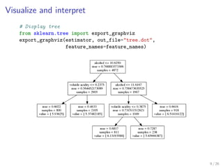
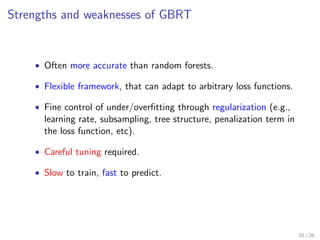
![Careful tuning required
from sklearn.ensemble import GradientBoostingRegressor
from sklearn.cross_validation import ShuffleSplit
from sklearn.grid_search import GridSearchCV
# Careful tuning is required to obtained good results
param_grid = {"learning_rate": [0.1, 0.01, 0.001],
"subsample": [1.0, 0.9, 0.8],
"max_depth": [3, 5, 7],
"min_samples_leaf": [1, 3, 5]}
est = GradientBoostingRegressor(n_estimators=1000)
grid = GridSearchCV(est, param_grid,
cv=ShuffleSplit(n=len(X), n_iter=10, test_size=0.25),
scoring="mean_squared_error",
n_jobs=-1).fit(X, y)
gbrt = grid.best_estimator_
See our PyData 2014 tutorial for further guidance
https://github.com/pprett/pydata-gbrt-tutorial
19 / 26](https://image.slidesharecdn.com/slides-150408072332-conversion-gate01/85/Tree-models-with-Scikit-Learn-Great-models-with-little-assumptions-22-320.jpg)

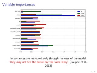
![Variable importances
importances = pd.DataFrame()
# Variable importances with Random Forest, default parameters
est = RandomForestRegressor(n_estimators=10000, n_jobs=-1).fit(X, y)
importances["RF"] = pd.Series(est.feature_importances_,
index=feature_names)
# Variable importances with Totally Randomized Trees
est = ExtraTreesRegressor(max_features=1, max_depth=3,
n_estimators=10000, n_jobs=-1).fit(X, y)
importances["TRTs"] = pd.Series(est.feature_importances_,
index=feature_names)
# Variable importances with GBRT
importances["GBRT"] = pd.Series(gbrt.feature_importances_,
index=feature_names)
importances.plot(kind="barh")
21 / 26](https://image.slidesharecdn.com/slides-150408072332-conversion-gate01/85/Tree-models-with-Scikit-Learn-Great-models-with-little-assumptions-25-320.jpg)
![Partial dependence plots
Relation between the response Y and a subset of features,
marginalized over all other features.
from sklearn.ensemble.partial_dependence import plot_partial_dependence
plot_partial_dependence(gbrt, X,
features=[1, 10], feature_names=feature_names)
23 / 26](https://image.slidesharecdn.com/slides-150408072332-conversion-gate01/85/Tree-models-with-Scikit-Learn-Great-models-with-little-assumptions-27-320.jpg)
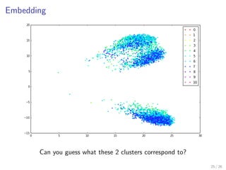
![Embedding
from sklearn.ensemble import RandomTreesEmbedding
from sklearn.decomposition import TruncatedSVD
# Project wines through a forest of totally randomized trees
# and use the leafs the samples end into as a high-dimensional representation
hasher = RandomTreesEmbedding(n_estimators=1000)
X_transformed = hasher.fit_transform(X)
# Plot wines on a plane using the 2 principal components
svd = TruncatedSVD(n_components=2)
coords = svd.fit_transform(X_transformed)
n_values = 10 + 1 # Wine preferences are from 0 to 10
cm = plt.get_cmap("hsv")
colors = (cm(1. * i / n_values) for i in range(n_values))
for k, c in zip(range(n_values), colors):
plt.plot(coords[y == k, 0], coords[y == k, 1], ’.’, label=k, color=c)
plt.legend()
plt.show()
24 / 26](https://image.slidesharecdn.com/slides-150408072332-conversion-gate01/85/Tree-models-with-Scikit-Learn-Great-models-with-little-assumptions-28-320.jpg)

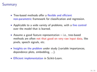


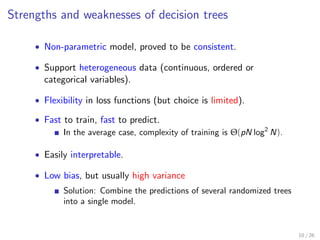
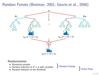
The document discusses tree-based models in machine learning, focusing on decision trees, random forests, and gradient boosted regression trees, emphasizing their applicability to regression and classification tasks using the scikit-learn library. It outlines the mechanics of these models, including their strengths and weaknesses, and illustrates tuning and validation techniques for optimizing performance. The document also highlights the importance of feature representation and offers insights into model interpretability through variable importances and partial dependence plots.