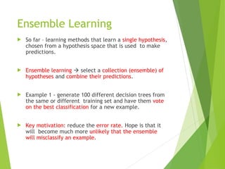
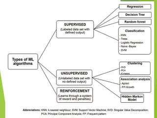
Ensemble Learning
Sofar – learning methods that learn a single hypothesis,
chosen from a hypothesis space that is used to make
predictions.
Ensemble learning select a collection (ensemble) of
hypotheses and combine their predictions.
Example 1 - generate 100 different decision trees from
the same or different training set and have them vote
on the best classification for a new example.
Key motivation: reduce the error rate. Hope is that it
will become much more unlikely that the ensemble
will misclassify an example.
18.
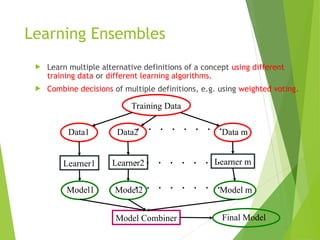
Learning Ensembles
Learnmultiple alternative definitions of a concept using different
training data or different learning algorithms.
Combine decisions of multiple definitions, e.g. using weighted voting.
Training Data
Data1 Data m
Data2
Learner1 Learner2 Learner m
Model1 Model2 Model m
Model Combiner Final Model
19.
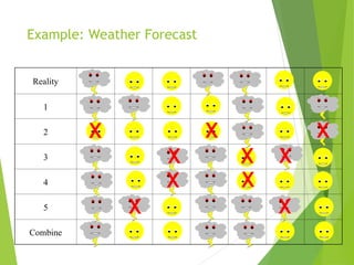
Value of Ensembles
“No Free Lunch” Theorem
No single algorithm wins all the time!
When combing multiple independent and diverse
decisions each of which is at least more accurate than
random guessing, random errors cancel each other out,
correct decisions are reinforced.
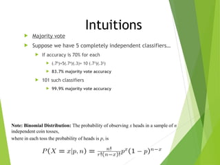
Majority vote
Suppose we have 5 completely independent classifiers…
If accuracy is 70% for each
(.75
)+5(.74
)(.3)+ 10 (.73
)(.32
)
83.7% majority vote accuracy
101 such classifiers
99.9% majority vote accuracy
Intuitions
Note: Binomial Distribution: The probability of observing x heads in a sample of n
independent coin tosses,
where in each toss the probability of heads is p, is
22.
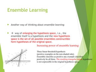
Ensemble Learning
Anotherway of thinking about ensemble learning:
way of enlarging the hypothesis space, i.e., the
ensemble itself is a hypothesis and the new hypothesis
space is the set of all possible ensembles constructible
form hypotheses of the original space.
Increasing power of ensemble learning:
Three linear threshold hypothesis
(positive examples on the non-shaded side);
Ensemble classifies as positive any example classified
positively be all three. The resulting triangular region hypothesis
is not expressible in the original hypothesis space.
23.
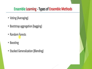
Different types ofensemble
learning
Different learning algorithms
Algorithms with different choice for parameters
Data set with different features (e.g. random subspace)
Data set = different subsets (e.g. bagging, boosting)
24.
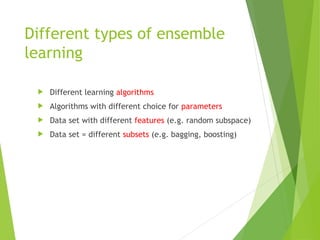
Different types ofensemble learning
(1)
Different algorithms, same set of training data
Training
Set L
A1
A2
An
…
C1
C2
Cn
…
A: algorithm I; C: classifier
25.
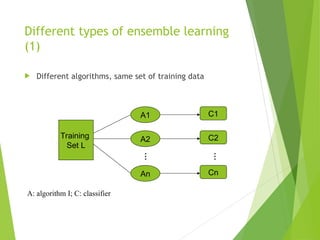
P1
Different types ofensemble learning
(2)
Same algorithm, different parameter settings
Training
Set L
A
C1
C2
Cn
P2
Pn
…
P: parameters for the learning algorithm
26.
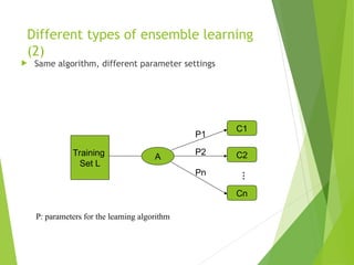
Different types ofensemble learning
(3)
Same algorithm, different versions of data set, e.g.
Bagging: resample training data
Boosting: Reweight training data
Decorate: Add additional artificial training data
RandomSubSpace (random forest): random subsets of features
Training
Set L
A
… C1
C2
Cn
…
L1
L2
Ln
In WEKA, these are called meta-learners, they take a learning
algorithm as an argument (base learner) and create a new learning
algorithm.
27.
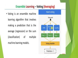
Combining an ensembleof
classifiers (1)
Voting:
Classifiers are combined in a static way
Each base-level classifier gives a (weighted) vote for its
prediction
Plurality vote: each base-classifier predict a class
Class distribution vote: each predict a probability
distribution
pC(x) = ΣCC pC(x) / | C |
28.
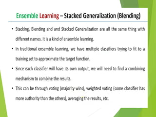
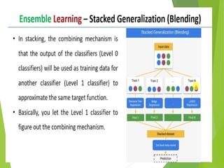
Combining an ensembleof
classifiers (2)
Stacking: a stack of classifiers
Classifiers are combined in a dynamically
A machine learning method is used to learn how to combine the
prediction of the base-level classifiers.
Top level classifier is used to obtain the final prediction from the
predictions of the base-level classifiers
29.
Combining an ensembleof
classifiers (3)
Cascading:
Combine classifiers iteratively.
At each iteration, training data set is extended with the
prediction obtained in the previous iteration
30.
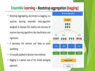
Bagging
Create ensemblesby “bootstrap aggregation”, i.e.,
repeatedly randomly resampling the training data
(Brieman, 1996).
Bootstrap: draw N items from X with replacement
Each bootstrap sample will on average contain 63.2%
of the unique training examples, the rest are replicates.
Bagging
Train M learners on M bootstrap samples
Combine outputs by voting (e.g., majority vote)
Decreases error by decreasing the variance in the results
due to unstable learners, algorithms (like decision trees
and neural networks) whose output can change
dramatically when the training data is slightly changed.
31.
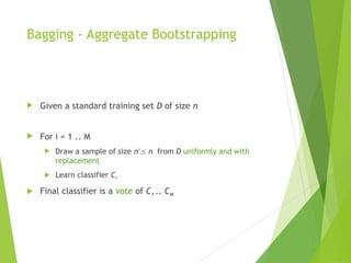
Bagging - AggregateBootstrapping
Given a standard training set D of size n
For i = 1 .. M
Draw a sample of size n*
n from D uniformly and with
replacement
Learn classifier Ci
Final classifier is a vote of C1 .. CM
32.
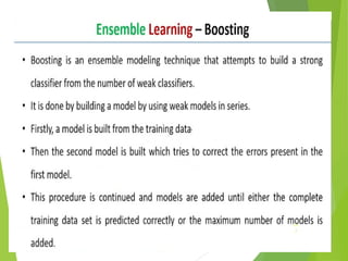
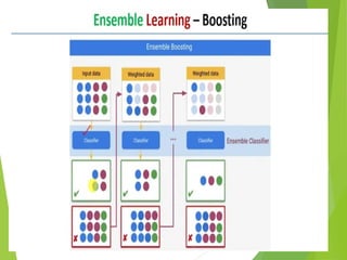
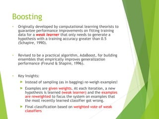
Boosting
• Originally developedby computational learning theorists to
guarantee performance improvements on fitting training
data for a weak learner that only needs to generate a
hypothesis with a training accuracy greater than 0.5
(Schapire, 1990).
• Revised to be a practical algorithm, AdaBoost, for building
ensembles that empirically improves generalization
performance (Freund & Shapire, 1996).
• Key Insights:
Instead of sampling (as in bagging) re-weigh examples!
Examples are given weights. At each iteration, a new
hypothesis is learned (weak learner) and the examples
are reweighted to focus the system on examples that
the most recently learned classifier got wrong.
Final classification based on weighted vote of weak
classifiers
33.
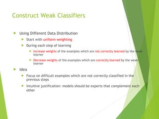
Construct Weak Classifiers
Using Different Data Distribution
Start with uniform weighting
During each step of learning
Increase weights of the examples which are not correctly learned by the weak
learner
Decrease weights of the examples which are correctly learned by the weak
learner
Idea
Focus on difficult examples which are not correctly classified in the
previous steps
Intuitive justification: models should be experts that complement each
other
34.
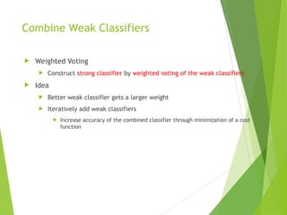
Combine Weak Classifiers
Weighted Voting
Construct strong classifier by weighted voting of the weak classifiers
Idea
Better weak classifier gets a larger weight
Iteratively add weak classifiers
Increase accuracy of the combined classifier through minimization of a cost
function
35.
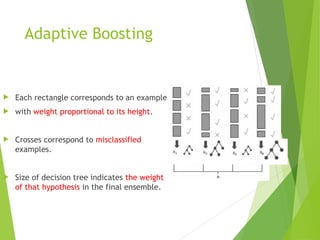
Adaptive Boosting
Eachrectangle corresponds to an example,
with weight proportional to its height.
Crosses correspond to misclassified
examples.
Size of decision tree indicates the weight
of that hypothesis in the final ensemble.
36.
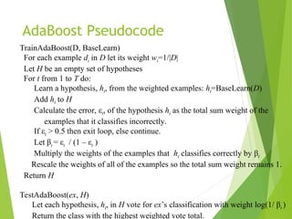
AdaBoost Pseudocode
TrainAdaBoost(D, BaseLearn)
Foreach example di in D let its weight wi=1/|D|
Let H be an empty set of hypotheses
For t from 1 to T do:
Learn a hypothesis, ht, from the weighted examples: ht=BaseLearn(D)
Add ht to H
Calculate the error, εt, of the hypothesis ht as the total sum weight of the
examples that it classifies incorrectly.
If εt > 0.5 then exit loop, else continue.
Let βt = εt / (1 – εt )
Multiply the weights of the examples that ht classifies correctly by βt
Rescale the weights of all of the examples so the total sum weight remains 1.
Return H
TestAdaBoost(ex, H)
Let each hypothesis, ht, in H vote for ex’s classification with weight log(1/ βt )
Return the class with the highest weighted vote total.
37.
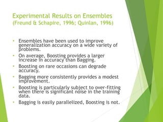
Experimental Results onEnsembles
(Freund & Schapire, 1996; Quinlan, 1996)
• Ensembles have been used to improve
generalization accuracy on a wide variety of
problems.
• On average, Boosting provides a larger
increase in accuracy than Bagging.
• Boosting on rare occasions can degrade
accuracy.
• Bagging more consistently provides a modest
improvement.
• Boosting is particularly subject to over-fitting
when there is significant noise in the training
data.
• Bagging is easily parallelized, Boosting is not.
38.
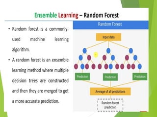
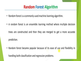
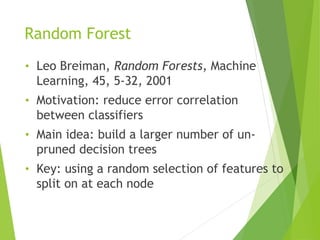
Random Forest
• LeoBreiman, Random Forests, Machine
Learning, 45, 5-32, 2001
• Motivation: reduce error correlation
between classifiers
• Main idea: build a larger number of un-
pruned decision trees
• Key: using a random selection of features to
split on at each node
39.
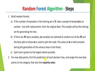
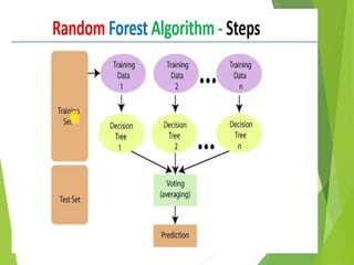
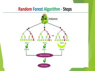
How Random ForestWork
• Each tree is grown on a bootstrap sample of the
training set of N cases.
• A number m is specified much smaller than the
total number of variables M (e.g. m = sqrt(M)).
• At each node, m variables are selected at
random out of the M.
• The split used is the best split on these m
variables.
• Final classification is done by majority vote
across trees.
39
40.
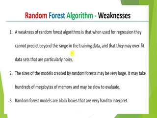
Advantages of randomforest
• Error rates compare favorably to Adaboost
• More robust with respect to noise.
• More efficient on large data
• Provides an estimation of the importance of
features in determining classification
• More info at:
http://stat-www.berkeley.edu/users/breiman/RandomForests/cc_ho
me.htm
41.
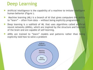
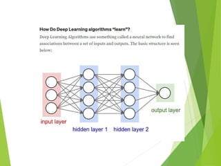
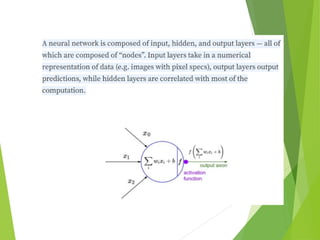
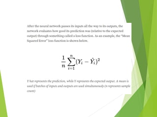
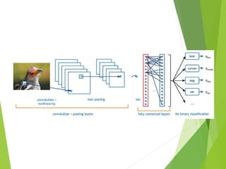
Deep Learning
Artificialintelligence is the capability of a machine to imitate intelligent
human behavior (Figure ).
Machine learning (ML) is a branch of AI that gives computers the ability
to “learn” — often from data — without being explicitly programmed.
Deep learning is a subfield of ML that uses algorithms called artificial
neural networks (ANNs), which are inspired by the structure and function
of the brain and are capable of self-learning.
ANNs are trained to “learn” models and patterns rather than being
explicitly told how to solve a problem