Unit V -Multiple Learners in artificial intelligence and machine learning

Multiple Learners
Prepared by: Nivetha R
Department of Computer Science and
Engineering

Multiple Learners
• There is no algorithm that is always the most accurate
• Generate a group of base-learners which when combined has higher
accuracy
• Different learners use different
• Algorithms
• Hyperparameters
• Representations /Modalities/Views
• Training sets

Voting – Hard and Soft Voting

Error-Correcting Output Codes
1. Classification Task:
o It is divided into multiple subtasks. Instead of solving one large classification problem, it is broken down
into simpler binary classification problems.
2. Simpler Classification Problems:
o Each binary classifier (a model that outputs either -1 or +1) focuses on a specific aspect of the task, helping
to simplify the overall problem.
3. Binary Classifiers:
o Each classifier outputs either -1 or +1. These outputs correspond to the class predictions for specific parts
of the task.
4. Code Matrix (W):
o A matrix W is introduced with K rows and L columns.
o The rows represent the different classes, and the columns correspond to different classifiers (base-
learners).
o The values within the matrix are binary (-1 or +1), which act as the "codes" for each class. Each class is
represented as a unique combination of -1s and +1s across the classifiers.

•One per class
L=K
•Pairwise
L=K(K-1)/2





























1
1
1
1
1
1
1
1
1
1
1
1
1
1
1
1
W

























1
1
0
1
0
0
1
0
1
0
1
0
0
1
1
0
0
1
0
0
0
1
1
1
W

Types of ECOC
• There are several variations of ECOC, each with its own characteristics and applications.
• One-vs-All (OvA): In the One-vs-All approach, each class is compared against all other classes.
This results in a code matrix where each column has one class labeled as 1 and all others as -1.
This method is simple but may not be optimal for all problems.
• One-vs-One (OvO): In the One-vs-One approach, each pair of classes is compared, resulting in a
code matrix where each column represents a binary classifier for a pair of classes. This method can
be more accurate but requires training more classifiers.
• Dense and Sparse Codes: Dense codes use a larger number of binary classifiers, resulting in more
robust error correction but higher computational cost. Sparse codes use fewer classifiers, reducing
computational cost but potentially sacrificing some robustness.

Advantages of Error Correcting Output Codes(ECOC)
• Robustness to Errors:
• Improved Generalization
• Flexibility
Applications of Error Correcting Output Codes(ECOC)
1. Image Classification
2. Text Classification
3. Bioinformatics
4. Speech Recognition

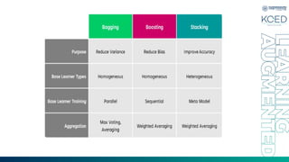
Bagging
What Is Bagging?
Bagging, an abbreviation for Bootstrap Aggregating, is a machine learning
ensemble strategy for enhancing the reliability and precision of predictive models. It
entails generating numerous subsets of the training data by employing random
sampling with replacement. These subsets train multiple base learners, such as
decision trees, neural networks, or other models.
During prediction, the outputs of these base learners are aggregated, often by
averaging (for regression tasks) or voting (for classification tasks), to produce the
final prediction. Bagging helps to reduce overfitting by introducing diversity among
the base learners and improves the overall performance by reducing variance and
increasing robustness

Bagging
•Use bootstrapping to generate L training sets
and train one base-learner with each (Breiman,
1996)
•Use voting (Average or median with regression)
•Unstable algorithms profit from bagging

Steps of Bagging
Dataset Preparation: Prepare your dataset, ensuring it's properly cleaned
and preprocessed. Split it into a training set and a test set.
Bootstrap Sampling: Randomly sample from the training dataset with
replacement to create multiple bootstrap samples. Each bootstrap sample
should typically have the same size as the original dataset, but some data
points may be repeated while others may be omitted.
Model Training: Train a base model (e.g., decision tree, neural network, etc.)
on each bootstrap sample. Each model should be trained independently of
the others.
Prediction Generation: Use each trained model to predict the test dataset.
Combining Predictions: Combine the predictions from all the models. You
can use majority voting to determine the final predicted class for classification
tasks. For regression tasks, you can average the predictions.

Bagging method
Bootstrap Aggregating is an ensemble learning technique that integrates many models to
produce a more accurate and robust prediction model. The following stages are included in
the bagging algorithm:
Bootstrap Sampling– It’s the process of randomly sampling a dataset with replacement to
generate various subsets known as bootstrap samples. The size of each subset is the same
as the original dataset.
Base Model Training– A base model, such as a decision tree or a neural network, is trained
individually on each bootstrap sample. Because the subsets are not similar, each base
model generates a separate prediction model.
Aggregation– The result of each base model is then aggregated via aggregation, which is
commonly accomplished by taking the average for regression problems or the mode for
classification issues. This aggregation process contributes to the reduction of variance and
the improvement of the generalization performance of the final prediction model.
Prediction– The completed model is used to forecast fresh data

Steps of Bagging
Evaluation: Evaluate the bagging ensemble's performance on the test dataset
using appropriate metrics (e.g., accuracy, F1 score, mean squared error, etc.).
Hyperparameter Tuning: If necessary, tune the hyperparameters of the base
model(s) or the bagging ensemble itself using techniques like cross-validation.
Deployment: Once you're satisfied with the performance of the bagging
ensemble, deploy it to make predictions on new, unseen data.

Boosting
The term ‘Boosting’ refers to a family of algorithms
which converts weak learner to strong learners.

How Does Boosting Algorithms
Work?
• Step 1: The base learner takes all the distributions and assign equal weight or
attention to each observation.
• Step 2: If there is any prediction error caused by first base learning algorithm,
then we pay higher attention to observations having prediction error. Then, we
apply the next base learning algorithm.
• Step 3: Iterate Step 2 till the limit of base learning algorithm is reached or higher
accuracy is achieved.
Finally, it combines the outputs from weak learner and creates a strong
learner which eventually improves the prediction power of the model.
Boosting pays higher focus on examples which are mis-classiﬁed or have
higher errors by preceding weak rules.

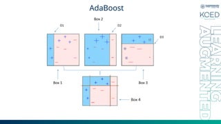
AdaBoost
• Box 1: You can see that we have assigned equal weights to each data point and
applied a decision stump to classify them as + (plus) or – (minus). The decision
stump (D1) has generated vertical line at left side to classify the data points. We
see that, this vertical line has incorrectly predicted three + (plus) as – (minus). In
such case, we’ll assign higher weights to these three + (plus) and apply another
decision stump.

AdaBoost
• Box 2: Here, you can see that the size of three incorrectly predicted + (plus) is
bigger as compared to rest of the data points. In this case, the second decision
stump (D2) will try to predict them correctly. Now, a vertical line (D2) at right side
of this box has classified three mis-classified + (plus) correctly. But again, it has
caused mis-classification errors. This time with three -(minus). Again, we will
assign higher weight to three – (minus) and apply another decision stump.

AdaBoost
• Box 3: Here, three – (minus) are given higher weights. A decision stump (D3) is
applied to predict these mis-classified observation correctly. This time a
horizontal line is generated to classify + (plus) and – (minus) based on higher
weight of mis-classified observation.

Stacking
• Stacked generalization is an ensemble method where a new model learns
how to best combine the predictions from multiple existing models
• In stacking, an algorithm takes the outputs of sub-models as input and
attempts to learn how to best combine the input predictions to make a
better output prediction.
• Can be Non Linear

Stacking
•Combiner f () is
another learner
(Wolpert, 1992)

Cascading
Use dj only if
preceding ones are
not confident
Cascade learners in
order of complexity

Key Components of Cascading
1.Stages:
1. Each stage typically consists of a classifier or model that operates on the
data.
2. Early stages use simpler models that quickly identify and discard obvious
negative samples.
3. Later stages employ more complex models that handle the remaining,
more challenging cases.
2.Decision Thresholds:
1. Each classifier in the cascade has a threshold that determines whether a
sample is classified positively or negatively.
2. The thresholds can be adjusted to balance sensitivity (true positive rate)
and specificity (true negative rate).
3.Error Focus:
1. Each subsequent model in the cascade is trained to focus on the errors
made by the previous classifiers, enhancing the overall model's ability to
correct mistakes.

How Cascading Works
1.Initial Classifier: The first model is trained on the entire dataset. It makes
predictions and classifies samples.
2.Filtering:
1. Samples that are classified as negatives are discarded.
2. Positive samples are passed to the next stage for further analysis.
3.Subsequent Classifiers:
1. Each subsequent classifier builds on the output of the previous one.
2. This continues until all stages have been applied or until a final decision is
made.

Cascading
• For example, suppose we want to build a machine learning model which would
detect if a credit card transaction is fraudulent or not.

Unit V -Multiple Learners in artificial intelligence and machine learning

More Related Content

Similar to Unit V -Multiple Learners in artificial intelligence and machine learning

Recently uploaded

Unit V -Multiple Learners in artificial intelligence and machine learning