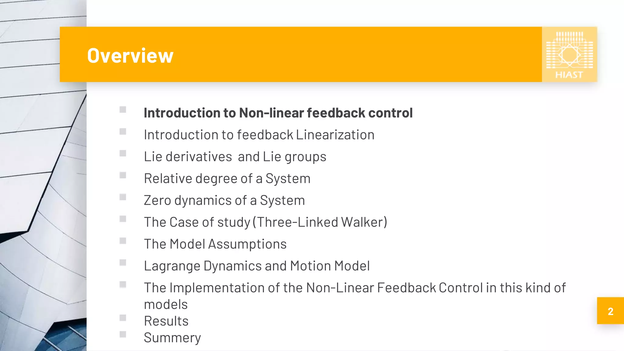
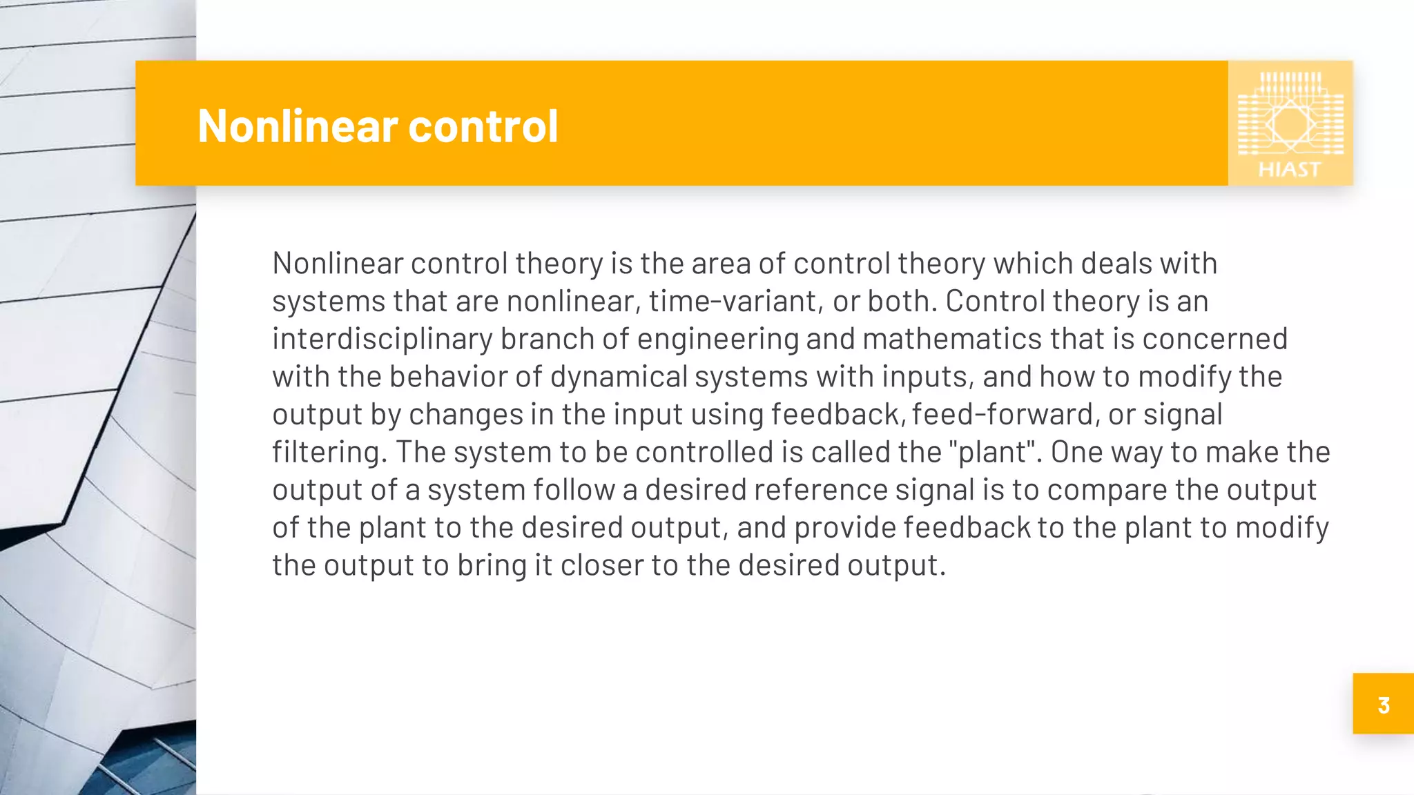
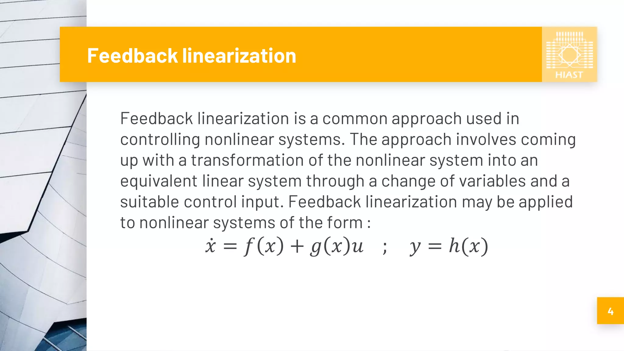
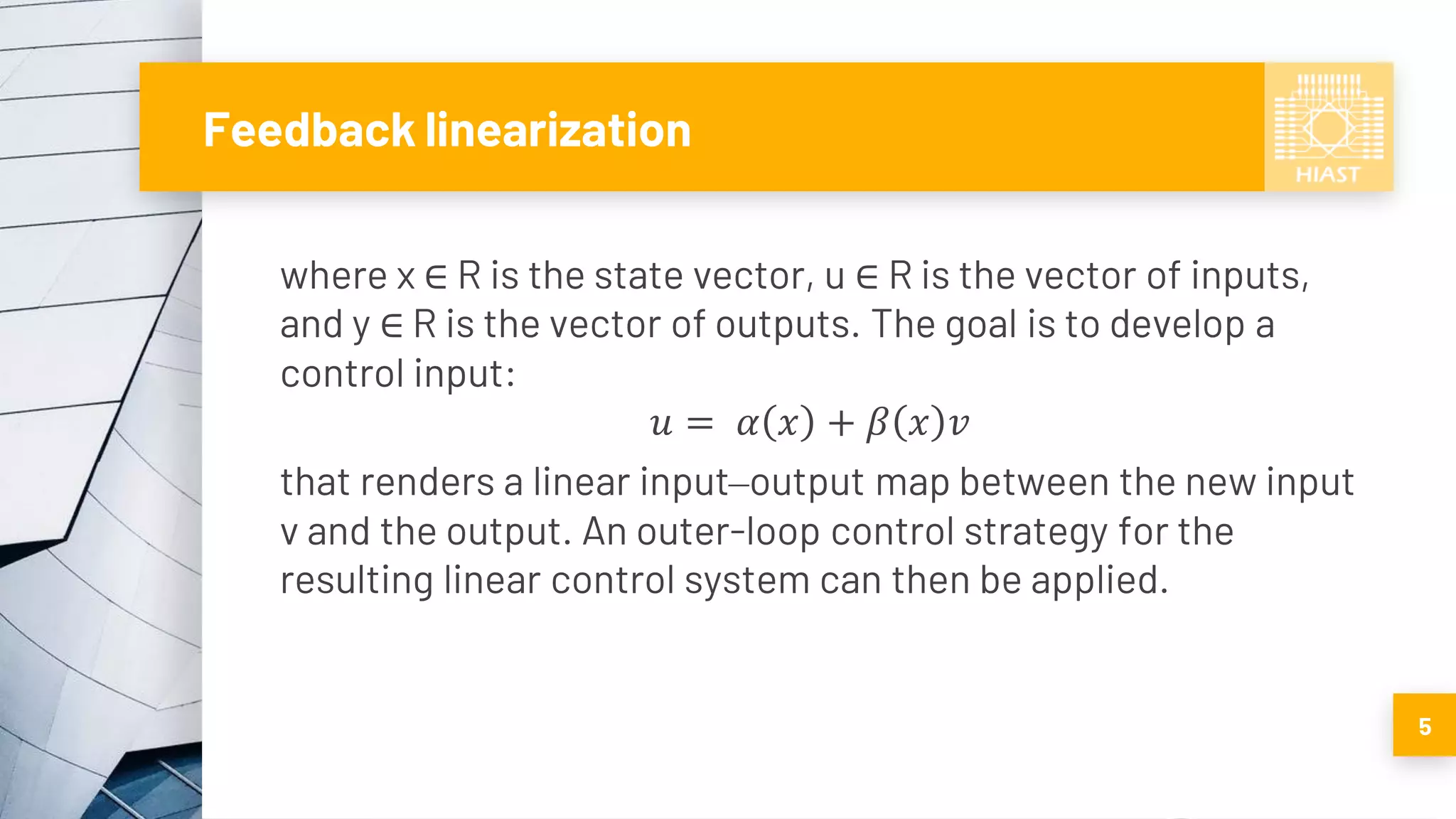
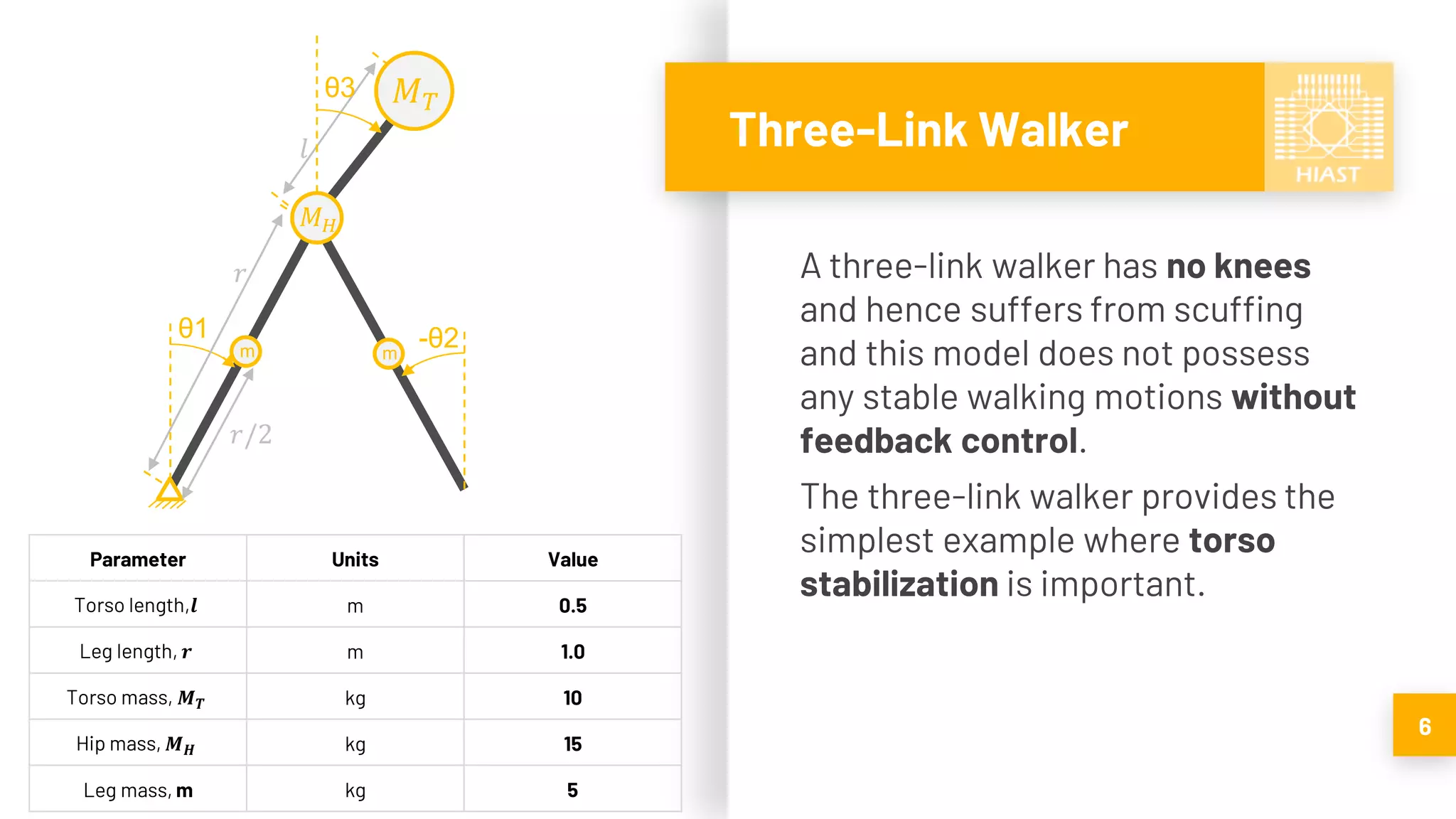
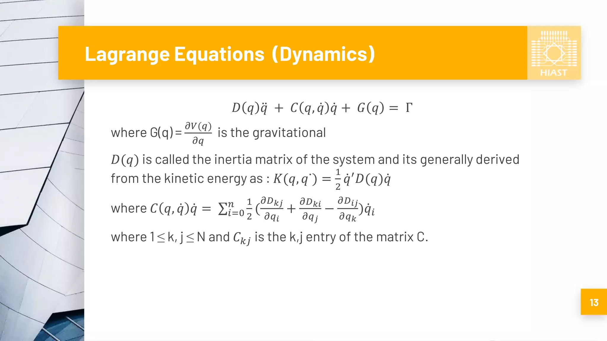
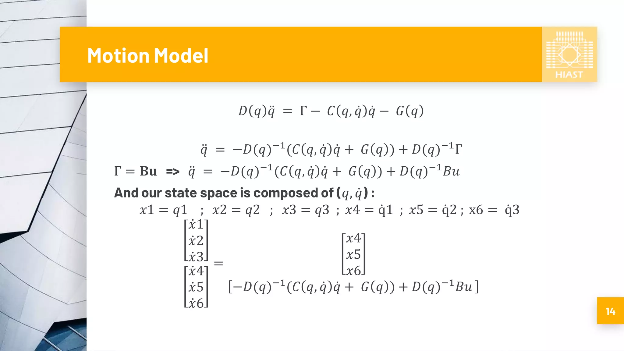
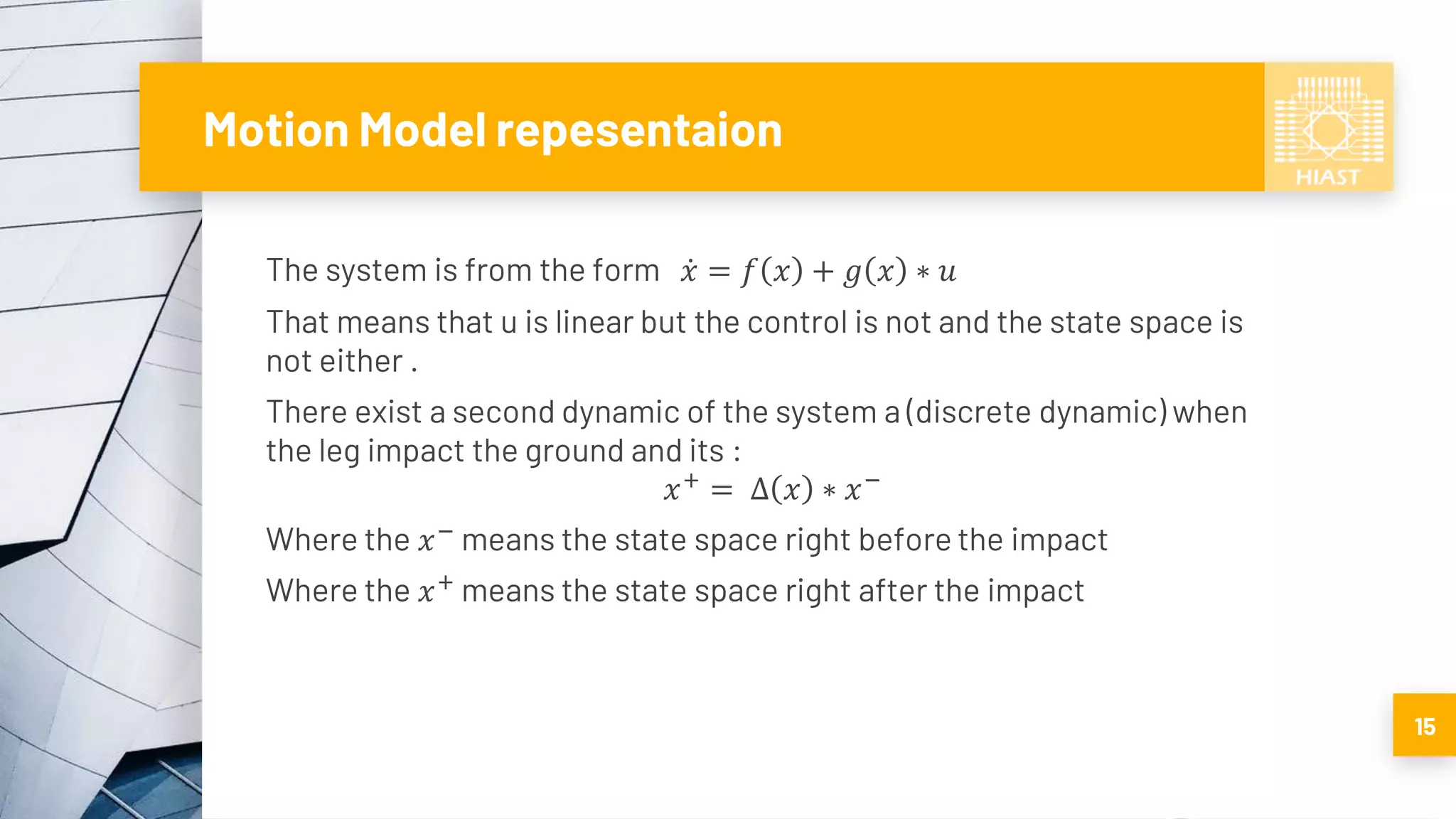
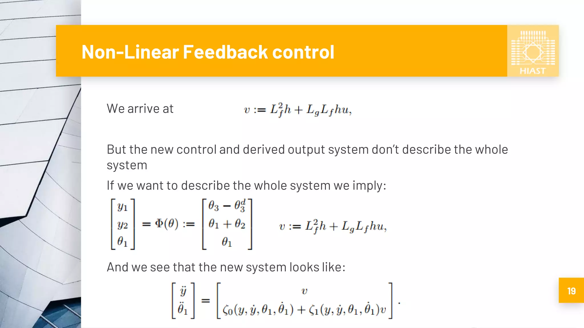
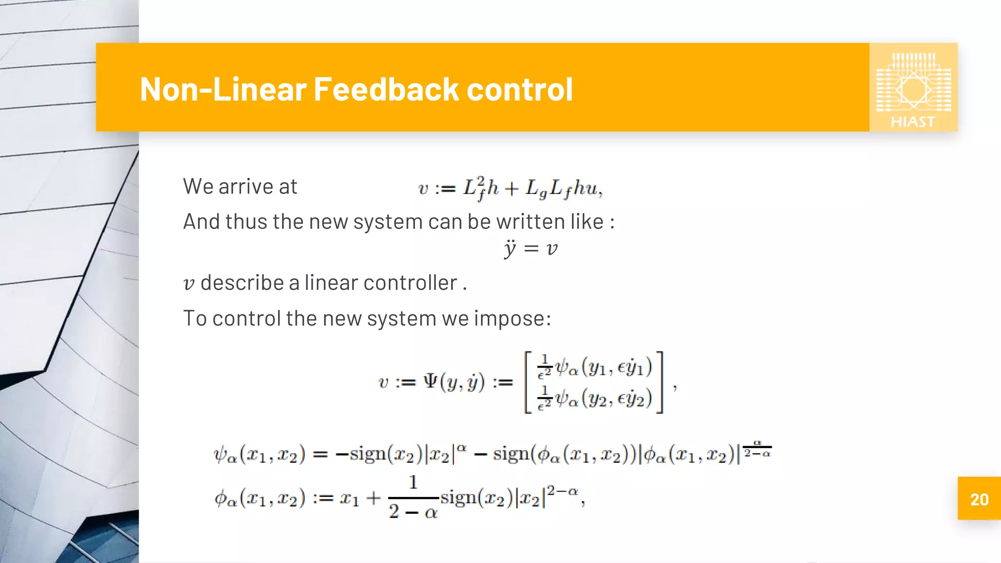
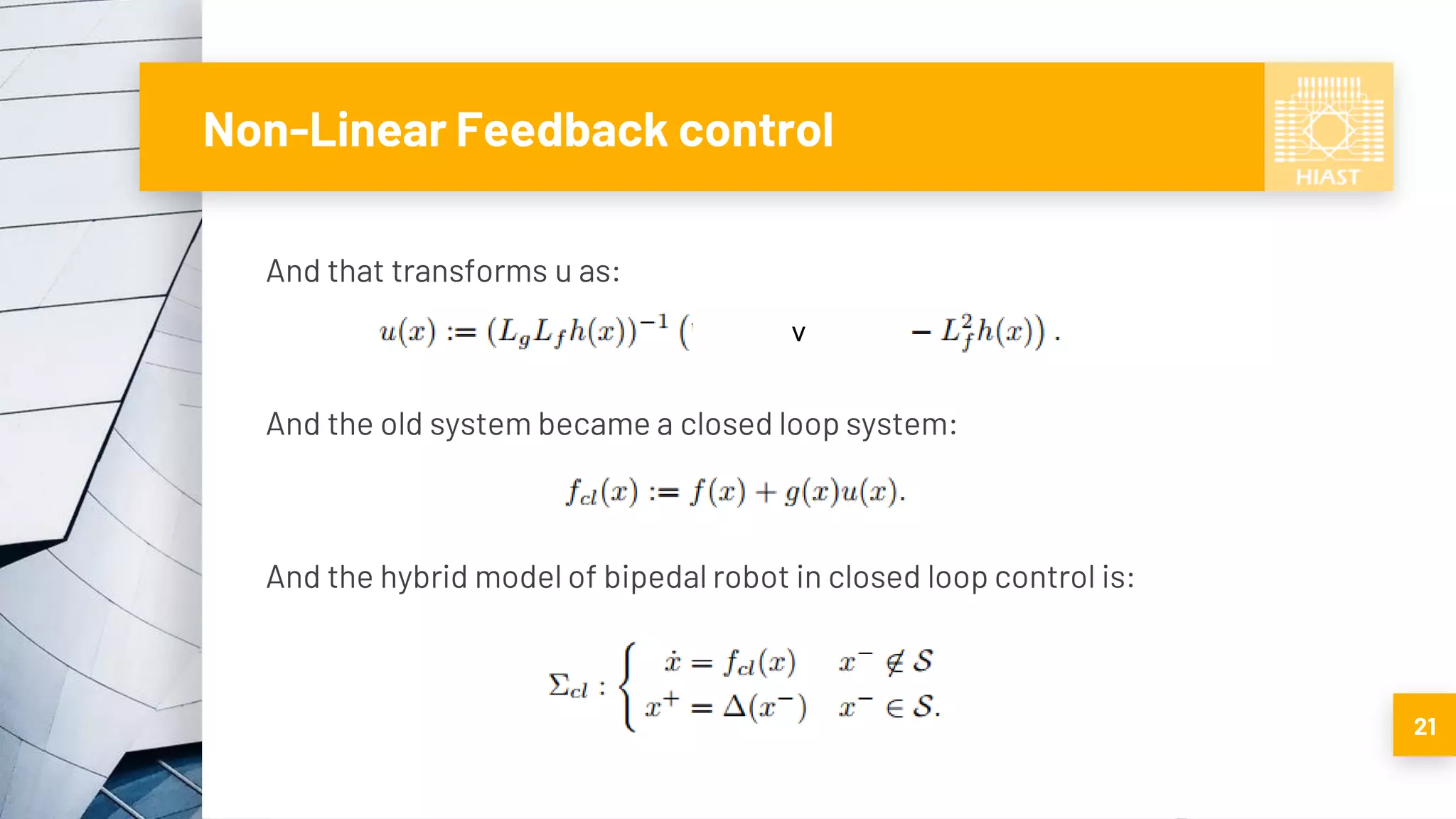
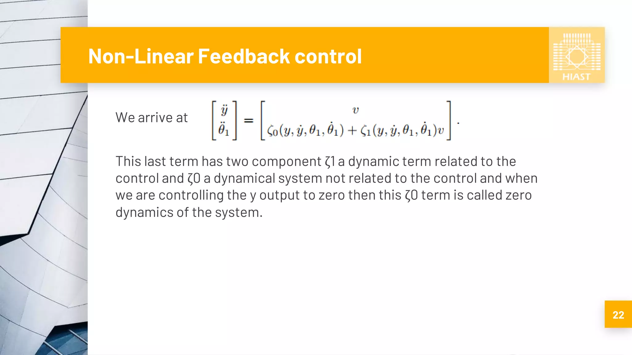
The document discusses the principles of non-linear control theory with a focus on controlling a three-link bipedal robot. Key topics include feedback linearization, Lagrangian dynamics, and the challenges of achieving stable walking motions. Results indicate that while the non-linear feedback controller can manage the robot's movements to some extent, direct control of the under-actuated system presents difficulties due to infinite amplitude errors in the motion model.

1. Bi-pedal Robot
Non-linear Control
by Eng. Mike Simon
Supervisor : Dr. Ibrahim chuaib
HIAST

2. Overview
▪ Introduction to Non-linear feedback control
▪ Introduction to feedback Linearization
▪ Lie derivatives and Lie groups
▪ Relative degree of a System
▪ Zero dynamics of a System
▪ The Case of study (Three-Linked Walker)
▪ The Model Assumptions
▪ Lagrange Dynamics and Motion Model
▪ The Implementation of the Non-Linear Feedback Control in this kind of
models
▪ Results
▪ Summery
2

3. Nonlinear control
Nonlinear control theory is the area of control theory which deals with
systems that are nonlinear, time-variant, or both. Control theory is an
interdisciplinary branch of engineering and mathematics that is concerned
with the behavior of dynamical systems with inputs, and how to modify the
output by changes in the input using feedback,feed-forward, or signal
filtering. The system to be controlled is called the "plant". One way to make the
output of a system follow a desired reference signal is to compare the output
of the plant to the desired output, and provide feedback to the plant to modify
the output to bring it closer to the desired output.
3

4. Feedback linearization
Feedback linearization is a common approach used in
controlling nonlinear systems. The approach involves coming
up with a transformation of the nonlinear system into an
equivalent linear system through a change of variables and a
suitable control input. Feedback linearization may be applied
to nonlinear systems of the form :
ሶ𝑥 = 𝑓 𝑥 + 𝑔 𝑥 𝑢 ; 𝑦 = ℎ(𝑥)
4

5. Feedback linearization
where x ∈ R is the state vector, u ∈ R is the vector of inputs,
and y ∈ R is the vector of outputs. The goal is to develop a
control input:
𝑢 = 𝛼 𝑥 + 𝛽 𝑥 𝑣
that renders a linear input–output map between the new input
v and the output. An outer-loop control strategy for the
resulting linear control system can then be applied.
5

6. Three-Link Walker
A three-link walker has no knees
and hence suffers from scuffing
and this model does not possess
any stable walking motions without
feedback control.
The three-link walker provides the
simplest example where torso
stabilization is important.
6
θ3
θ1 -θ2
𝑀 𝑇
𝑀 𝐻
m m
𝑙
𝑟
𝑟/2
Parameter Units Value
Torso length,𝒍 m 0.5
Leg length, 𝒓 m 1.0
Torso mass, 𝑴 𝑻 kg 10
Hip mass, 𝑴 𝑯 kg 15
Leg mass, m kg 5

7. Assumptions (Robot and point feet)
▪ comprised of 3 rigid links connected by 2 revolute joints to form a single
open kinematic chain.
▪ each link has nonzero mass and its mass is not distributed
(i.e., each link is modeled as a point mass). 
▪ planar, with motion constrained to the sagittal plane.
▪ bipedal, with two symmetric legs connected at a common point
called the hip, and both leg ends are terminated in points.
▪ independently actuated at each of the 2 revolute joints.
▪ unactuated at the point of contact between the stance leg and
ground.
7

8. Assumptions (Links and Joints)
▪ The robot will be modeled as connections of rigid links through revolute
joints, with all links lying in a common plane and the axes of rotation of
the joints being normal to the plane.
▪ each joint is further assumed to be ideal, meaning that the connection is
rigid and frictionless
▪ Finally, links are implicitly assumed to be noninterfering, meaning that,
magically, individual links can assume arbitrary positions and
orientations without contacting one another.
8

9. Assumptions (Walking)
▪ there are alternating phases of single support and impact
▪ during the single support phase, the stance leg end acts as an ideal pivot.
▪ at impact, the swing leg neither slips nor rebounds, while the former
stance leg releases without interaction with the ground.
▪ in each step, the swing leg starts from strictly behind the stance leg and
is placed strictly in front of the stance leg at impact.
▪ walking is from left to right and takes place on a level surface.
9

10. Lagrange Dynamics and Motion Model

11. Lagrange Equations (energy equations)
Instead of forces, Lagrangian mechanics uses the energies in the system. The central quantity of
Lagrangian mechanics is the Lagrangian, a function which summarizes the dynamics of the
entire system
Lagrangian for a system of particles can be defined by: 𝑳 = 𝑲 − 𝑽
Where K is the total kinetic energy of the system, equaling the sum Σ of the kinetic energies of the
smaller pieces of the system with respect to some fixed frame. Generally noted as:
𝑲 =
𝟏
𝟐
෍
𝒌=𝟏
𝒏
𝒎𝒗 𝟐
The potential energy of the system reflects the energy of conservative forces (e.g. Newtonian gravity)
its not always the case of Newtonian gravity But in the case of normal ridged body dynamics its noted
as:
𝑽 = 𝑴𝒕𝒐𝒕𝒂𝒍 ∗ 𝒈 ∗ 𝒑 𝒗 𝒄𝒐𝒎
11

12. Lagrange Equations (lagrangian)
The Lagrangian is the real-valued function given by the total kinetic energy minus the total
potential energy Lagrangian for a system of particles can be defined by: 𝑳 = 𝑲 − 𝑽
Lagrange’s equation is
𝑑
𝑑𝑡
𝜕𝐿
𝜕 ሶ𝑞
−
𝜕𝐿
𝜕𝑞
= Γ + σ 𝐹𝑒𝑥
where Γ is the vector of generalized torques and forces from the
actuator.
If the kinetic energy is quadratic, that is: 𝐾(𝑞, 𝑞˙) =
1
2
ሶ𝑞′
𝐷(𝑞) ሶ𝑞
then the Lagrange equation results in the second-order differential
equation
𝐷 𝑞 ሷ𝑞 + 𝐶 𝑞, ሶ𝑞 ሶ𝑞 + 𝐺 𝑞 = Γ
12

13. Lagrange Equations (Dynamics)
𝐷 𝑞 ሷ𝑞 + 𝐶 𝑞, ሶ𝑞 ሶ𝑞 + 𝐺 𝑞 = Γ
where G(q) =
𝜕𝑉(𝑞)
𝜕𝑞
is the gravitational
𝐷(𝑞) is called the inertia matrix of the system and its generally derived
from the kinetic energy as : 𝐾(𝑞, 𝑞˙) =
1
2
ሶ𝑞′
𝐷(𝑞) ሶ𝑞
where 𝐶 𝑞, ሶ𝑞 ሶ𝑞 = σ𝑖=0
𝑛 1
2
(
𝜕𝐷 𝑘𝑗
𝜕𝑞𝑖
+
𝜕𝐷 𝑘𝑖
𝜕𝑞 𝑗
−
𝜕𝐷 𝑖𝑗
𝜕𝑞 𝑘
) ሶ𝑞𝑖
where 1 ≤ k, j ≤ N and 𝐶 𝑘𝑗 is the k,j entry of the matrix C.
13

14. Motion Model
𝐷 𝑞 ሷ𝑞 = Γ − 𝐶 𝑞, ሶ𝑞 ሶ𝑞 − 𝐺 𝑞
ሷ𝑞 = −𝐷(𝑞)−1
(𝐶 𝑞, ሶ𝑞 ሶ𝑞 + 𝐺 𝑞 ) + 𝐷(𝑞)−1
Γ
Γ = 𝐁𝐮 => ሷ𝑞 = −𝐷(𝑞)−1
(𝐶 𝑞, ሶ𝑞 ሶ𝑞 + 𝐺 𝑞 ) + 𝐷(𝑞)−1
𝐵𝑢
And our state space is composed of (𝑞, ሶ𝑞) :
𝑥1 = 𝑞1 ; 𝑥2 = 𝑞2 ; 𝑥3 = 𝑞3 ; 𝑥4 = ሶq1 ; 𝑥5 = ሶq2 ; x6 = ሶq3
ሶ𝑥1
ሶ𝑥2
ሶ𝑥3
ሶ𝑥4
ሶ𝑥5
ሶ𝑥6
=
𝑥4
𝑥5
𝑥6
−𝐷(𝑞)−1
(𝐶 𝑞, ሶ𝑞 ሶ𝑞 + 𝐺 𝑞 ) + 𝐷(𝑞)−1
𝐵𝑢
14

15. Motion Model repesentaion
The system is from the form ሶ𝑥 = 𝑓 𝑥 + 𝑔 𝑥 ∗ 𝑢
That means that u is linear but the control is not and the state space is
not either .
There exist a second dynamic of the system a (discrete dynamic) when
the leg impact the ground and its :
𝑥+
= ∆ 𝑥 ∗ 𝑥−
Where the 𝑥−
means the state space right before the impact
Where the 𝑥+
means the state space right after the impact
15

16. Non-Linear Feedback control

17. Non-Linear Feedback control
We select h to view theta2 and theta3 the entities that we want to
control and we add to them the desired output because we want to
control them to zero of the output this leads to:
ℎ 𝑥 = 𝑥2 − 𝑥2𝑑𝑒𝑠𝑖𝑟𝑒𝑑 𝑥3 − 𝑥3𝑑𝑒𝑠𝑖𝑟𝑒𝑑
and we derive y 2 times (until the control terms kick in).
17

18. Non-Linear Feedback control
We select h to view theta2 and theta3 the entities that we want to
control and we add to them the desired output because we want to
control them to zero of the output this leads to:
ℎ 𝑥 = 𝑥2 − 𝑥2𝑑𝑒𝑠𝑖𝑟𝑒𝑑 𝑥3 − 𝑥3𝑑𝑒𝑠𝑖𝑟𝑒𝑑
and we derive y 2 times (until the control terms kick in).
18

19. Non-Linear Feedback control
We arrive at
But the new control and derived output system don’t describe the whole
system
If we want to describe the whole system we imply:
And we see that the new system looks like:
19

20. Non-Linear Feedback control
We arrive at
And thus the new system can be written like :
ሷ𝑦 = 𝑣
𝑣 describe a linear controller .
To control the new system we impose:
20

21. Non-Linear Feedback control
And that transforms u as:
And the old system became a closed loop system:
And the hybrid model of bipedal robot in closed loop control is:
21
v

22. Non-Linear Feedback control
We arrive at
This last term has two component ζ1 a dynamic term related to the
control and ζ0 a dynamical system not related to the control and when
we are controlling the y output to zero then this ζ0 term is called zero
dynamics of the system.
22

23. Results
Open Matlab for simulation
23

24. Summery
▪ The controls up until now has an infinite amplitude (maybe errors in
the motion model)
▪ Controlling this under-actuated system tells us that there exist a zero
dynamics in the system and it can’t be controlled directly using this
method.
▪ The non-linear feedback controller can control the robot to some
extend.
24

25. Refrences
-Feedback Control of Dynamic Bipedal Robot Locomotion book
- NonLinear Control via Input-Output Feedback Linearization of a
Robot Manipulator
Wafa Ghozlane*, Jilani Knani
- Non-linear control Normal Form Slides..
- Nonlinear Control Systems Slides
Ant´onio Pedro Aguiar
pedro@isr.ist.utl.pt
7. Feedback Linearization
IST-DEEC PhD Course
http://users.isr.ist.utl.pt/%7Epedro/NCS2012/
25