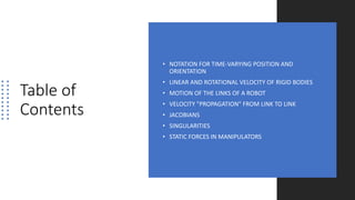
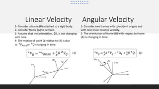
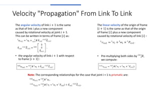
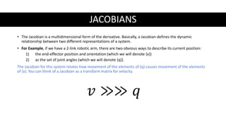
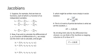
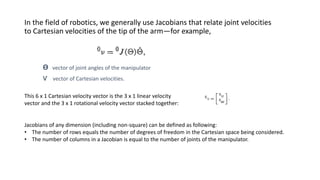
This document discusses robot dynamics and Jacobians. It covers: 1) Linear and rotational velocity of rigid bodies and how velocity propagates from link to link in a robot. 2) Jacobians relate how movement of joint angles causes movement of the end effector position and orientation. 3) Singularities occur when a robot loses degrees of freedom in Cartesian space. 4) Static forces in manipulators are analyzed by considering forces and torques exerted between links.

1. Robot Dynamics
Jacobians: velocities and static forces

2. Table of
Contents
• NOTATION FOR TIME-VARYING POSITION AND
ORIENTATION
• LINEAR AND ROTATIONAL VELOCITY OF RIGID BODIES
• MOTION OF THE LINKS OF A ROBOT
• VELOCITY "PROPAGATION" FROM LINK TO LINK
• JACOBIANS
• SINGULARITIES
• STATIC FORCES IN MANIPULATORS

3. Robot as Mechanisms
Robot
Open-Chain
Inverse
kinematics
Forward
kinematics
Closed-Chain
Inverse
kinematics
Forward
kinematics
Mixed-Chain
Kinematic Chain
Topology
Kinematic chain of a robot basically consists of:
Joint + Links

4. Kinematic chain of a robot basically consists of:
Joint + Links

5. Differentiation of Position Vectors

6. The angular velocity vector
We can think of angular velocity as describing rotational
motion of a frame that we attach to the body.
𝐴 𝛺 𝐵
: describes the rotation of frame (B} relative to {A}.
• Its direction indicates the instantaneous axis of rotation of {B} relative to {A},
and the magnitude of indicates the speed of rotation.

7. LINEAR AND ROTATIONAL
VELOCITY OF RIGID BODIES
• Motion of rigid bodies can be equivalently studied as
the motion of frames relative to one another.
• The notions of translations and orientations will be
extended to the time-varying case.

8. Linear Velocity Angular Velocity
1- Consider a frame (B) attached to a rigid body.
2- Consider frame {A} to be fixed.
3- Assume that the orientation, 𝐵
𝐴
𝑅, is not changing
with time.
4- The motion of point Q relative to (A} is due
to 𝐴
𝑃𝐵𝑜𝑟𝑔or 𝐵
𝑄 changing in time.
1- Consider two frames with coincident origins and
with zero linear relative velocity.
2- The orientation of frame {B} with respect to frame
{A} is changing in time.
(2)(1)

9. Simultaneous linear and rotational velocity
• We can very simply expand (2) to the case where origins are not coincident by adding on
the linear velocity of the origin to (2) to derive the general formula for velocity of a
vector fixed in frame {B} as seen from frame {A}:

10. MOTION OF THE
LINKS OF A ROBOT
Main Considerations:
• 1- Always use link frame {0} as our
reference frame.
• 2- 𝒗𝒊 is the linear velocity of the
origin of link frame {i}
• 3- 𝝎𝒊 is the angular velocity of link
frame {i}.
• 4- At any instant, each link of a
robot in motion has some linear
and angular velocity.

11. Velocity "Propagation"
From Link To Link
• A manipulator is a chain of bodies, each one
capable of motion relative to its neighbors.
Because of this structure, we can compute the
velocity of each link in order, starting from the
base.
• The velocity of link 𝑖 + 1 will be that of link 𝑖,
plus whatever new velocity components were
added by joint 𝑖 + 1
• Remember that linear velocity is associated
with a point, but angular velocity is associated
with a body. Hence, the term "velocity of a
link" here means the linear velocity of the
origin of the link frame and the rotational
velocity of the link.

12. Velocity "Propagation" From Link To Link
• the angular velocity of link 𝑖 + 1 with respect
to frame 𝑖 + 1 :
Note: The corresponding relationships for the case that joint i + 1 is prismatic are:
The linear velocity of the origin of frame
𝑖 + 1 is the same as that of the origin
of frame 𝑖 plus a new component
caused by rotational velocity of link 𝑖 ∶
• Pre-multiplying both sides by 𝑖
𝑖+1
𝑅,
we compute:
The angular velocity of link 𝑖 + 1 is the same
as that of link 𝑖 plus a new component
caused by rotational velocity at joint 𝑖 + 1.
This can be written in terms of frame {𝑖} as:

13. Example: A two-
link manipulator
• 1- start by attaching frames to
the links.
• 2- compute the velocity of the
origin of each frame, starting
from the base frame {0}, which
has zero velocity.
• 3- use the link transformations
to calculate the angular
velocities
• 4- To find the velocities with
respect to the nonmoving base
frame, we rotate them with the
rotation matrix 0
3
𝑅

14. JACOBIANS
• The Jacobian is a multidimensional form of the derivative. Basically, a Jacobian defines the dynamic
relationship between two different representations of a system.
• For Example, if we have a 2-link robotic arm, there are two obvious ways to describe its current position:
1) the end-effector position and orientation (which we will denote {x})
2) as the set of joint angles (which we will denote {q}).
The Jacobian for this system relates how movement of the elements of {q} causes movement of the elements
of {x}. You can think of a Jacobian as a transform matrix for velocity.
𝑣 ≫≫ 𝑞

15. Jacobians
1- Suppose, for example, that we have six
functions, each of which is a function of six
independent variables:
2- Now, if we wish to calculate the differentials of
𝑦𝑖 as a function of differentials of 𝑥𝑖, we simply
use the chain rule to calculate, and we get:
3- which might be written more simply in vector
notation:
4- The 6 x 6 matrix of partial derivatives is what we
call the Jacobian, J.
By dividing both sides by the differential time
element, we can think of the Jacobian as mapping
velocities in X to those in Y:

16. In the field of robotics, we generally use Jacobians that relate joint velocities
to Cartesian velocities of the tip of the arm—for example,
ϴ vector of joint angles of the manipulator
ѵ vector of Cartesian velocities.
This 6 x 1 Cartesian velocity vector is the 3 x 1 linear velocity
vector and the 3 x 1 rotational velocity vector stacked together:
Jacobians of any dimension (including non-square) can be defined as following:
• The number of rows equals the number of degrees of freedom in the Cartesian space being considered.
• The number of columns in a Jacobian is equal to the number of joints of the manipulator.

17. Changing A Jacobian's Frame Of Reference:
Given a Jacobian written in frame {B}, that is,
a 6 x 1 Cartesian velocity vector given in {B} is described relative to {A) by the
transformation
Hence, we can write
∴ changing the frame of reference of a Jacobian is accomplished by means of the
following relationship:

18. SINGULARITIES
1. Workspace-boundary singularities
• occur when the manipulator is fully
stretched out or folded back on itself
in such a way that the end-effector is
at or very near the boundary of the
workspace.
2. Workspace-interior singularities
• occur away from the workspace
boundary; they generally are caused
by a lining up of two or more joint
axes.
When a manipulator is in a singular configuration, it has lost one or more degrees of freedom (as viewed from
Cartesian space). This means that there is some direction (or subspace) in Cartesian space along which it is
impossible to move the hand of the robot, no matter what joint rates are selected.
To check for singularity we ask an important question: Is the Jacobian invertible for all values of ϴ? If not,
where is it not invertible?
Because if jacobine matrix invertible That means it is nonsingular.

19. STATIC FORCES IN MANIPULATORS
We define special symbols for the force and torque exerted by a neighbor link:
𝑓𝑖 = force exerted on link 𝑖 by link 𝑖 − 1
𝑛𝑖 = torque exerted on link 𝑖 by link 𝑖 − 1.
In the equilibrium state:
- sum of the forces is equal to zero.
- Sum of the torques about the origin of frame {i} is equal to zero
In order to write these equations in terms of only forces and
moments defined within their own link frames, we transform with
the rotation matrix describing frame {i + 1} relative to frame {i}.
This leads to our most important result for static force
"propagation" from link to link:

20. Joint Torque
• Torques are needed at the joints in order to balance the reaction forces and moments acting on
the links.
• The joint torque required to maintain the static equilibrium, the dot product of the joint-axis
vector with the moment vector acting on the link is computed:
• In the case that joint i is prismatic, we compute the joint actuator force as:

21. Manipulator Dynamics

22. Robot
Dynamics In the past lectures we discussed
the kinematics of the robots which
dealt with the static positions,
forces and velocities without taking
into account the forces required to
case the motion.
In this lecture we are going to
discuss the Robot Dynamics:
‘Robot dynamics is the relationship
between the forces acting on a
robot and the resulting motion of
the robot.’

23. The dynamic
model of a
manipulator
plays an
important role
for
• 1- Control algorithm
• 2- Simulation of motion
• 3- Analysis of manipulator structure

24. The Control Problem
• In This problem, we are given a trajectory
point, ϴ, Ӫ and ϴ. And we wish to find the
required vector of joint torques, τ.
• This formulation of dynamics is useful for
the problem of controlling the manipulator.

25. Simulation Of Motion
Problem
• Simulating manipulator motion allows control
strategies and motion planning techniques to be
tested without the need to use a physically
available system.
• In simulation we try to calculate how the
mechanism will move under application of a set
of joint torques.
• That is, given a torque vector, τ, calculate the
resulting motion of the manipulator, ϴ, Ӫ and ϴ.
This is useful for simulating the manipulator.

26. Analysis of manipulator
structure
• The analysis of the dynamic model can be
helpful for mechanical design of prototype
arms.
• Computation of the forces and torques
required for the execution of typical
motions provides useful information for
designing joints, transmissions and
actuators.

27. Evaluation of
the Equation
of Motion
There are two methods for derivation of the
equations of motion of a manipulator in the joint
space:
1. The first method is based on the Lagrange
formulation and is conceptually simple and
systematic.
2. The second method is based on the Newton–
Euler formulation and yields the model in a
recursive form;

28. Any Questions …