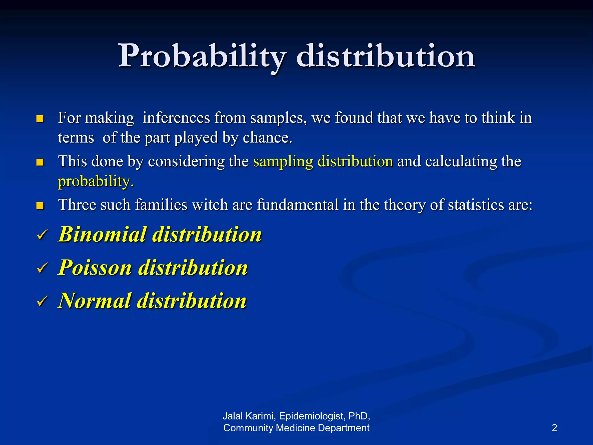
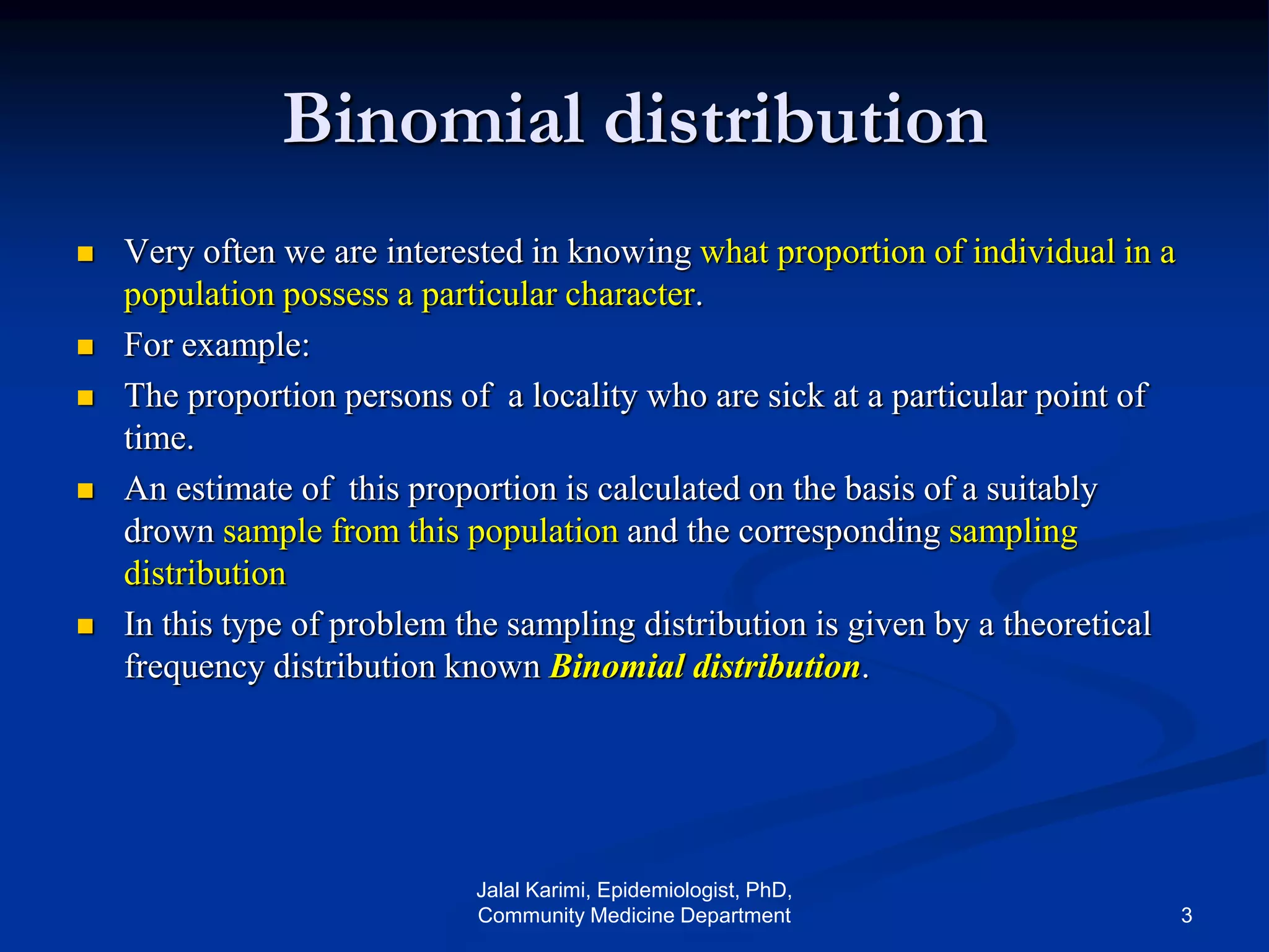
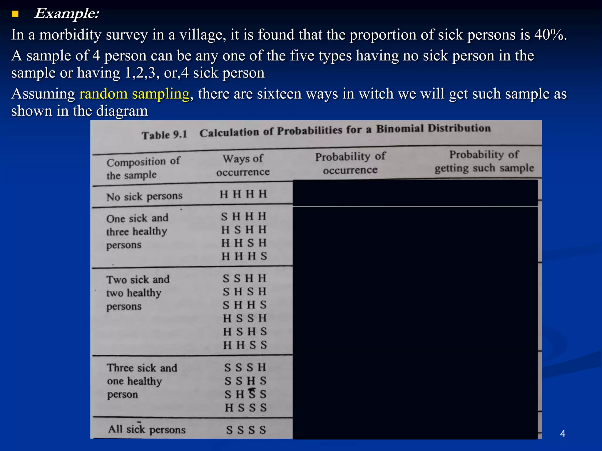
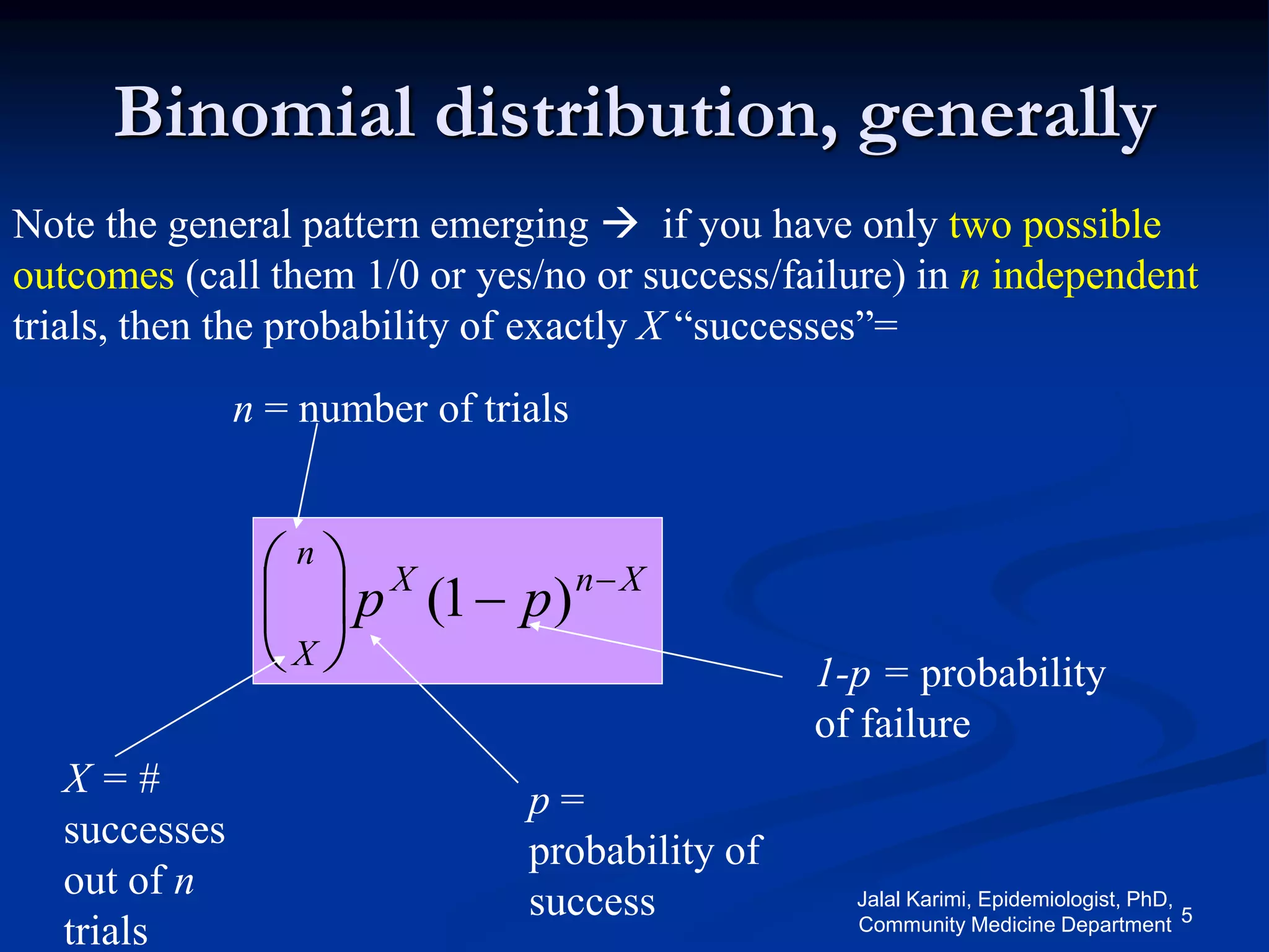
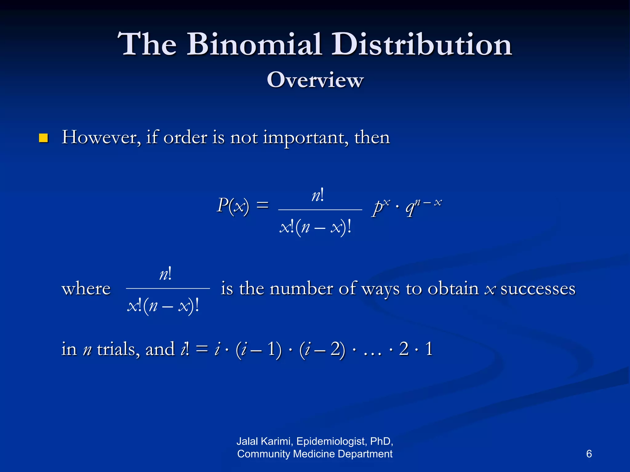
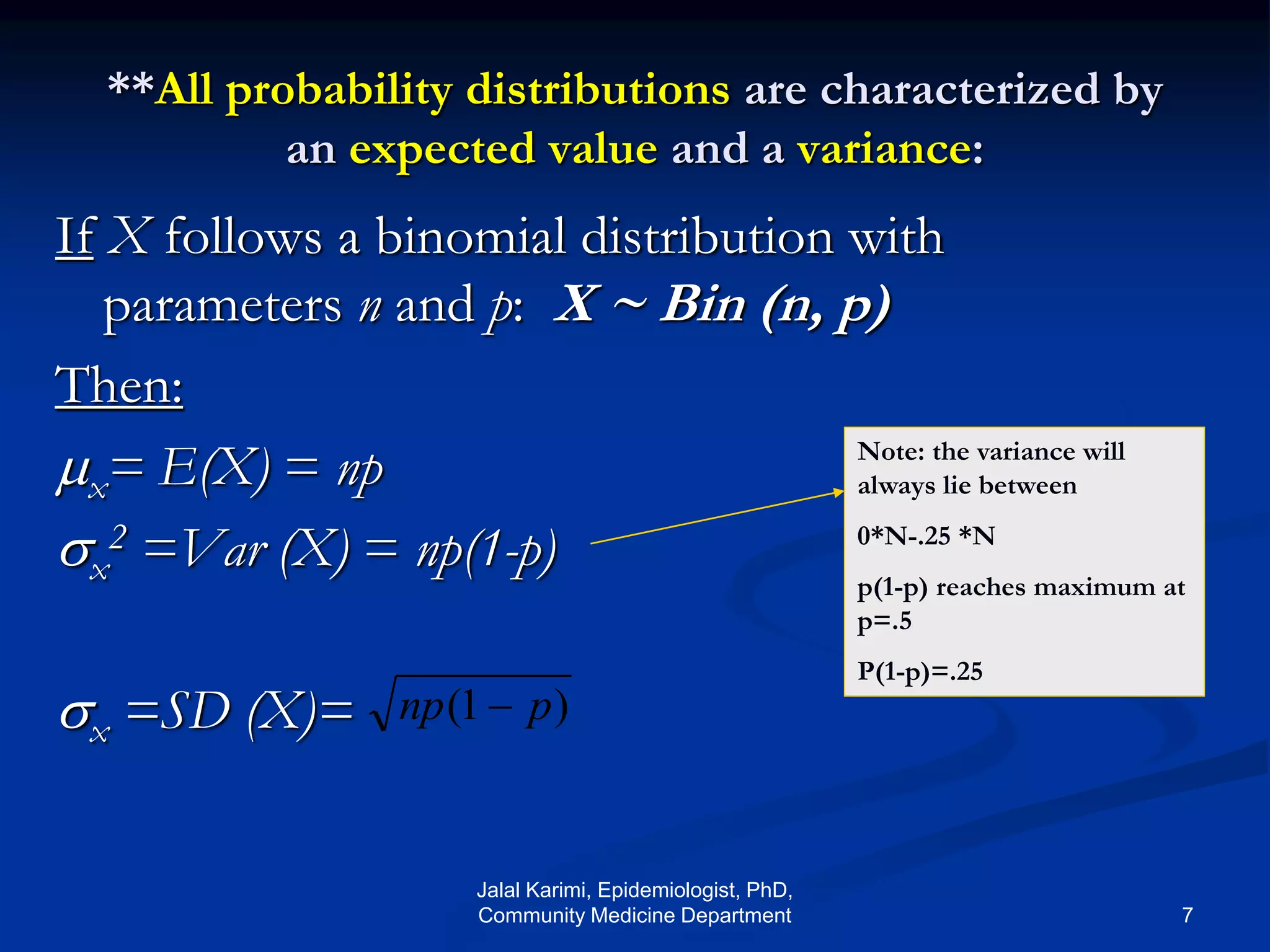
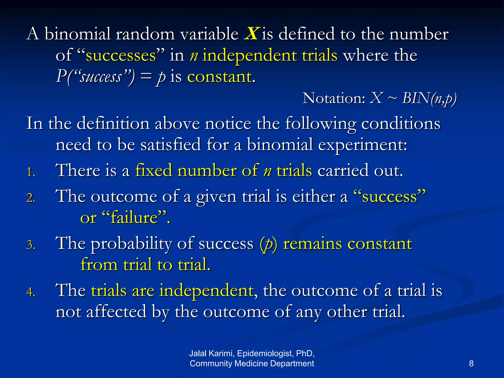
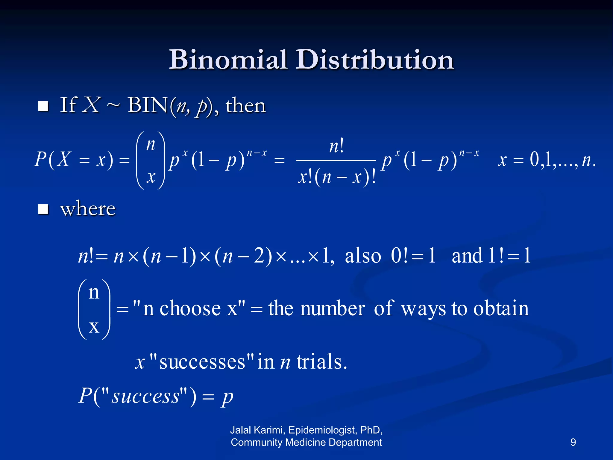
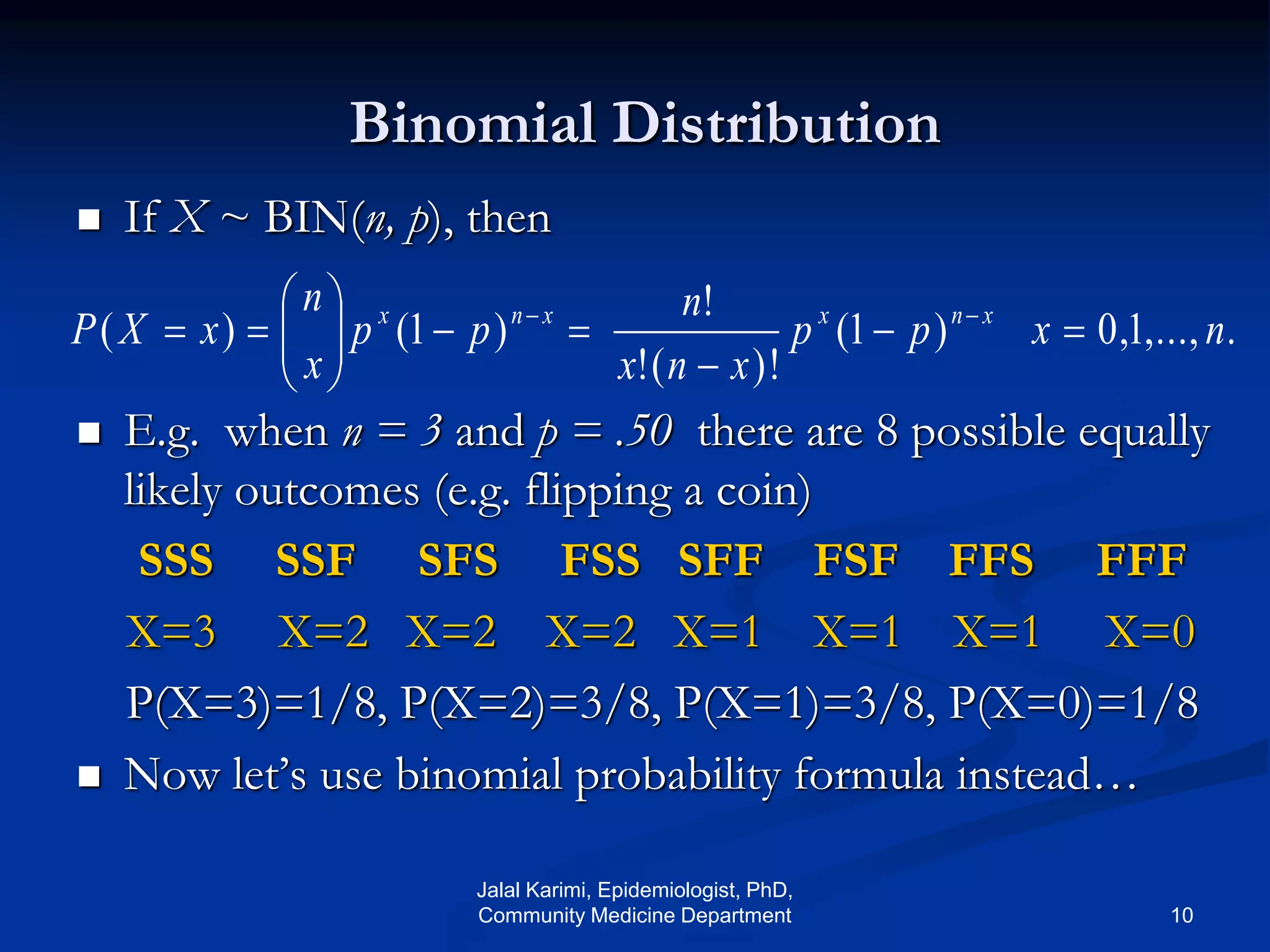
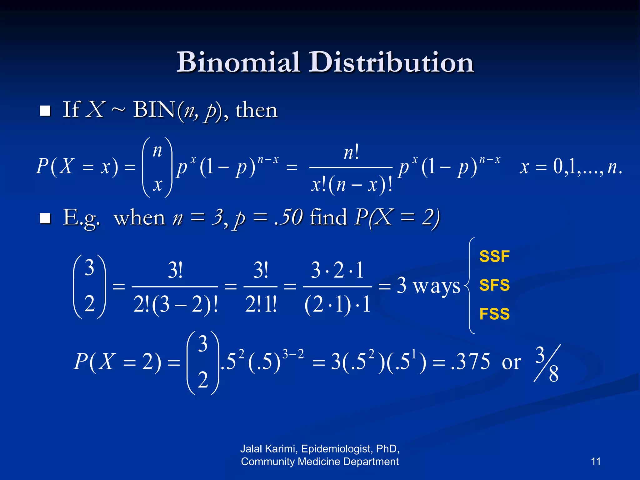
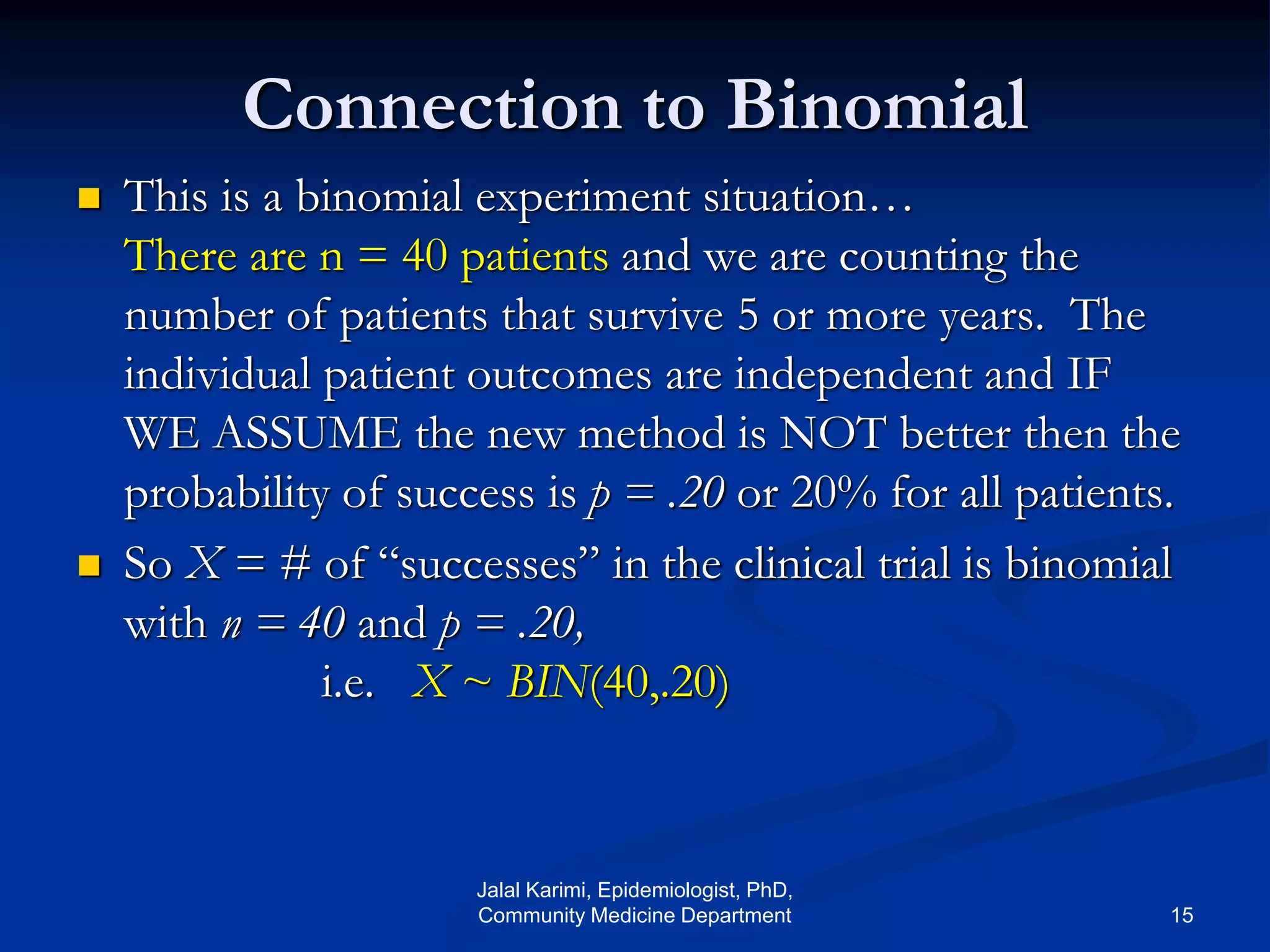
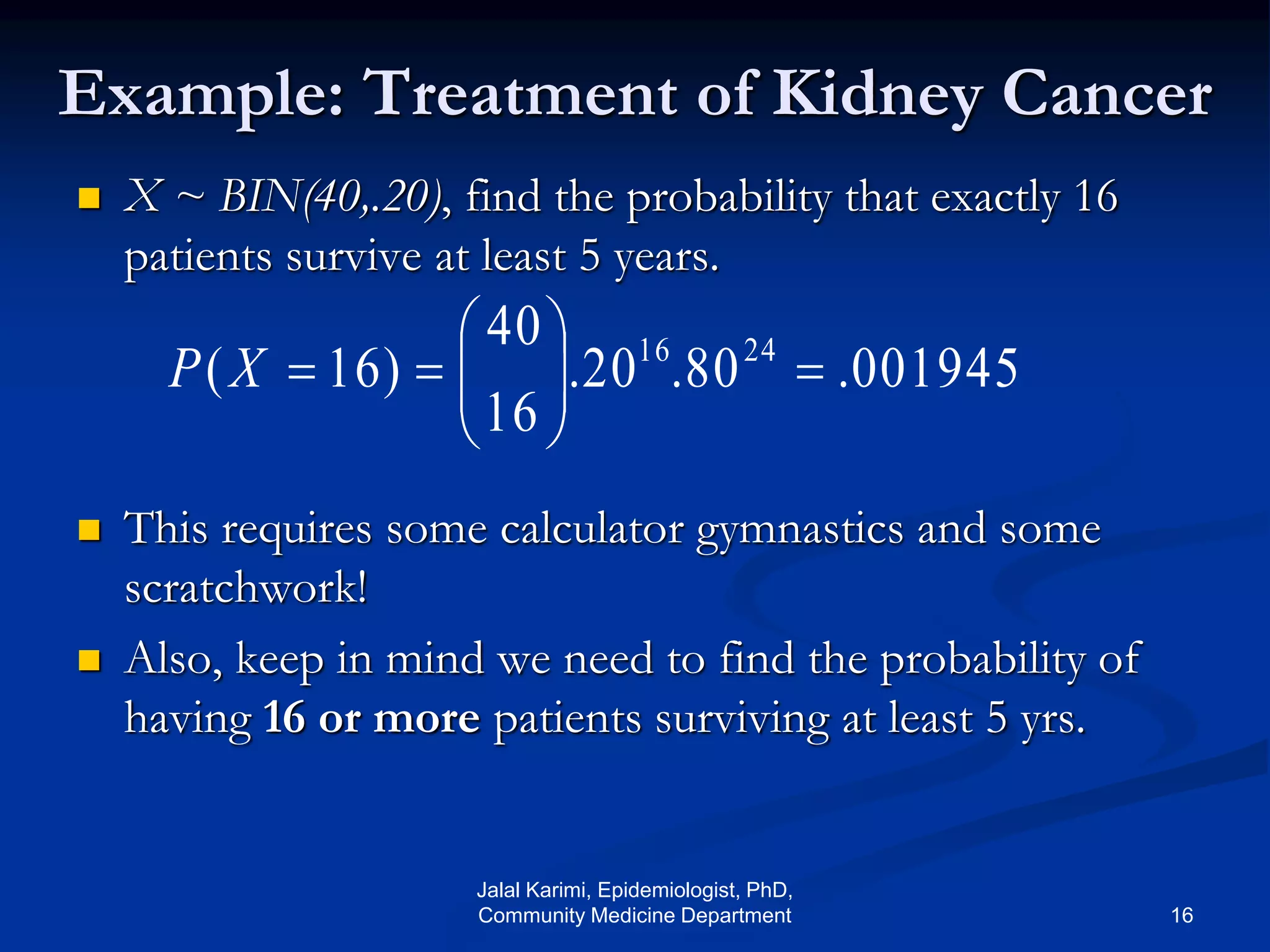
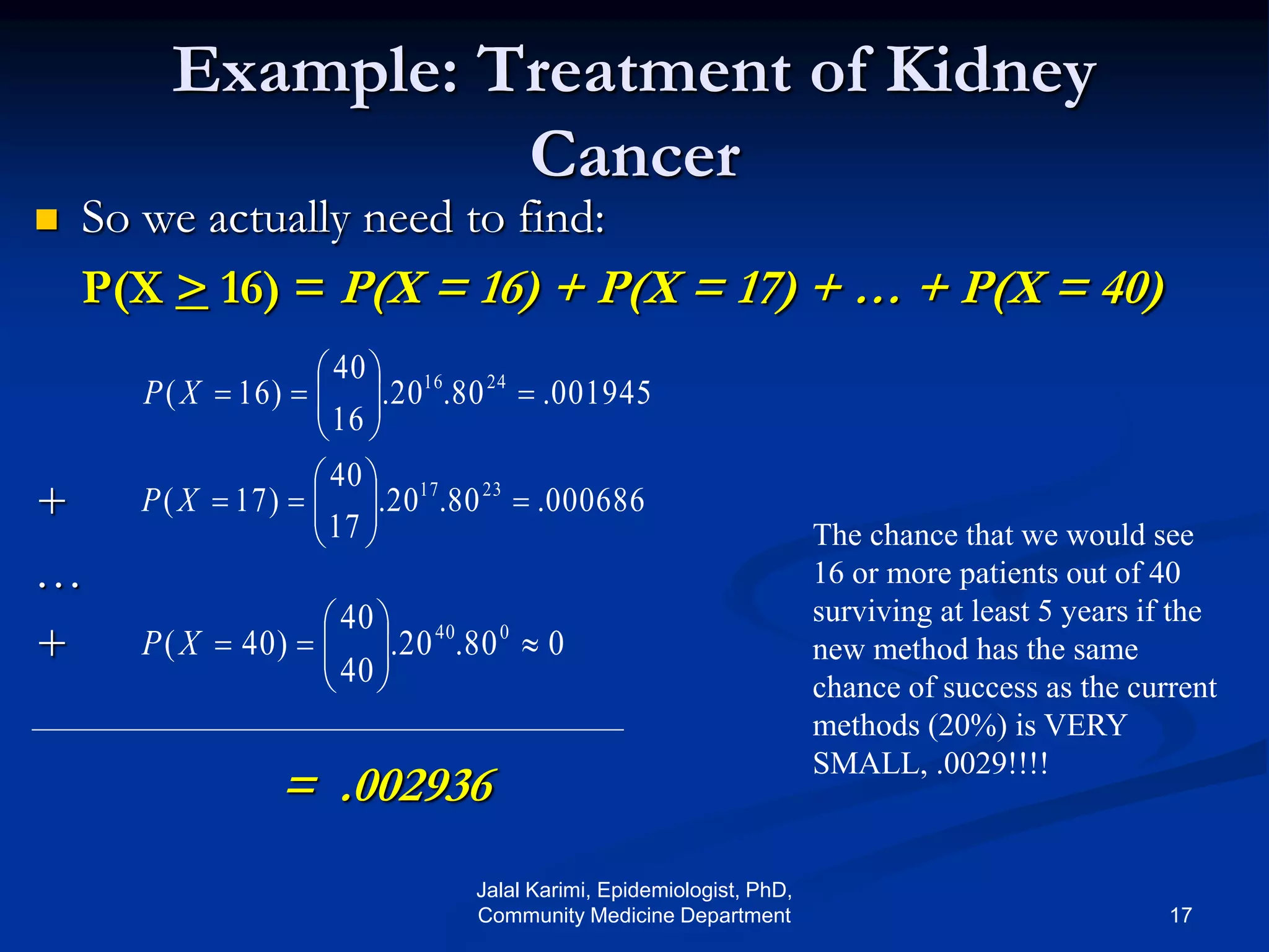
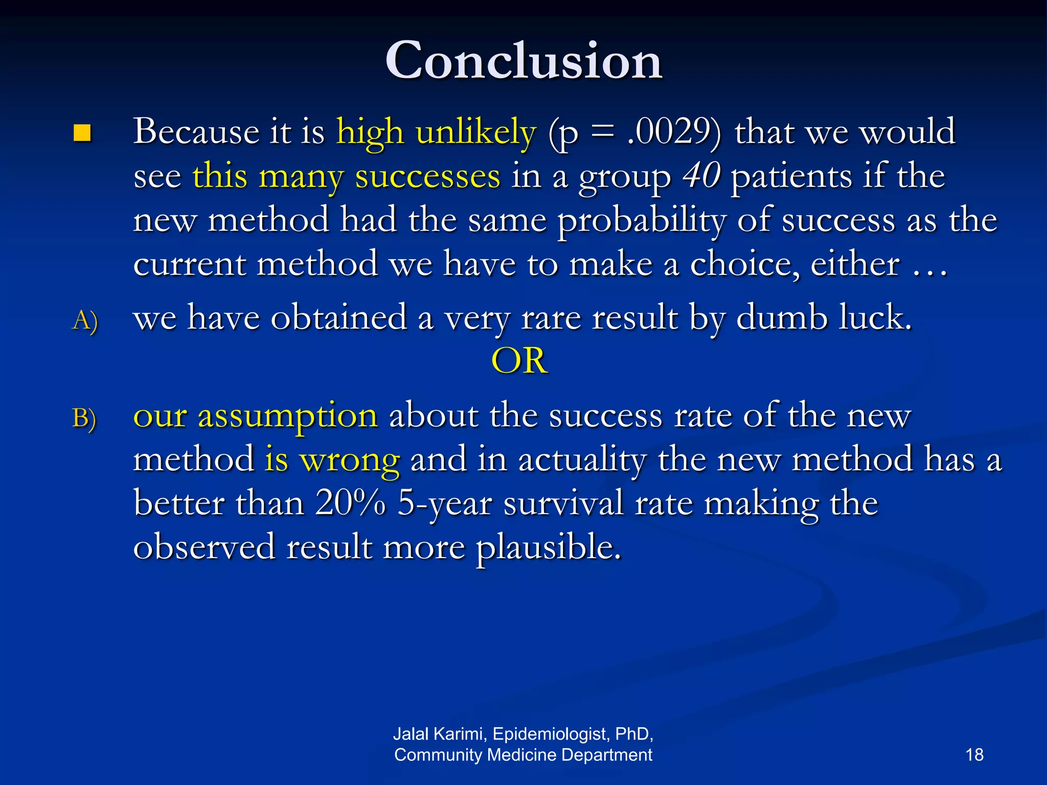
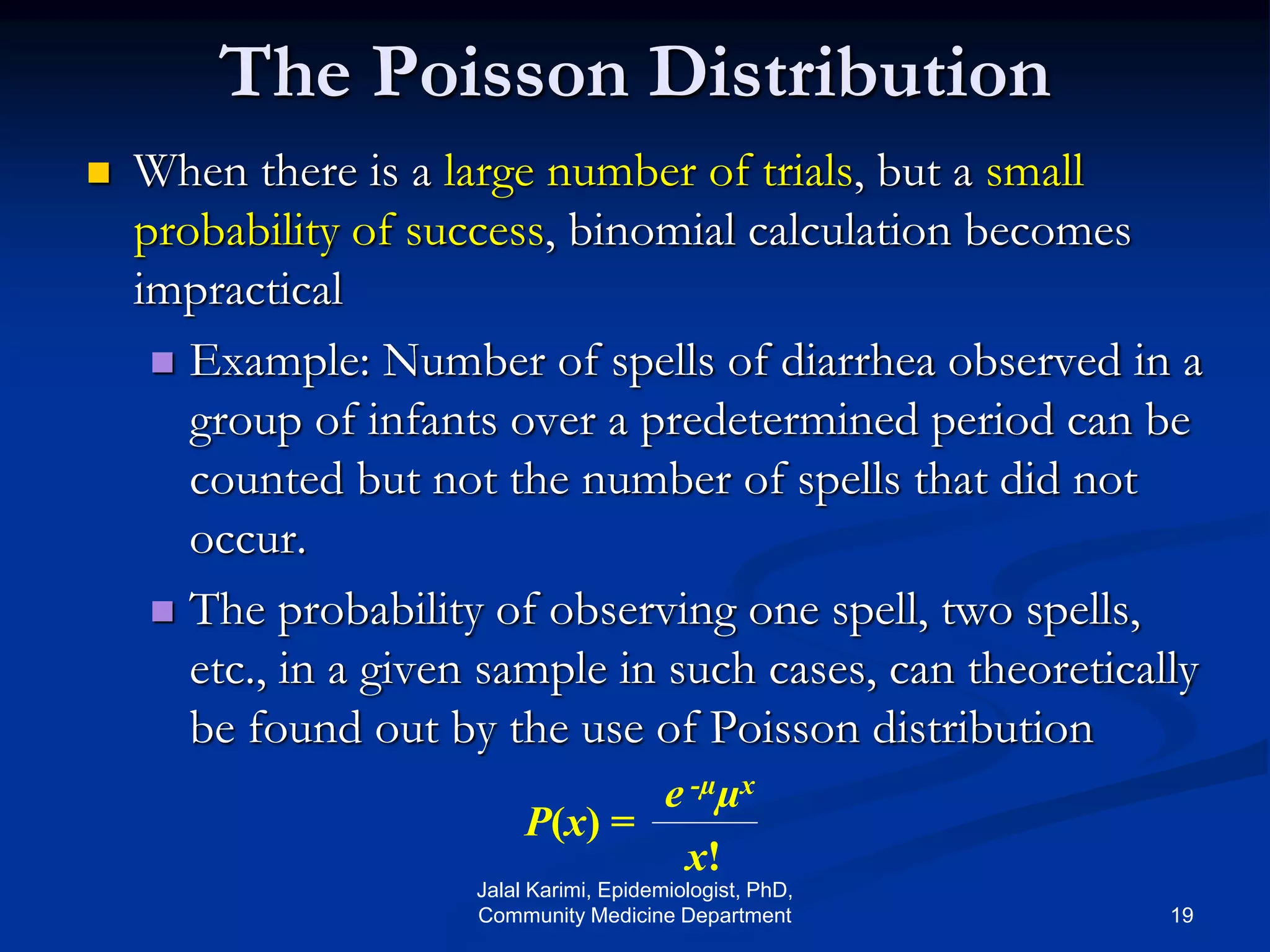
SlideShare a Scribd company logo
Biostatistics
Introduction to BIOSTATISTICS
Lecturer:
Jalal Karimi, MSc, PhD of Epidemiology
Reference:
Introduction to Biostatistics and Research Methods, Fifth Edition
By Sunder Rao
Department of Community Medicine
Third session
Jalal Karimi, Epidemiologist, PhD,
Community Medicine Department 1
Probability distribution
 For making inferences from samples, we found that we have to think in
terms of the part played by chance.
 This done by considering the sampling distribution and calculating the
probability.
 Three such families witch are fundamental in the theory of statistics are:
 Binomial distribution
 Poisson distribution
 Normal distribution
Jalal Karimi, Epidemiologist, PhD,
Community Medicine Department 2
Binomial distribution
 Very often we are interested in knowing what proportion of individual in a
population possess a particular character.
 For example:
 The proportion persons of a locality who are sick at a particular point of
time.
 An estimate of this proportion is calculated on the basis of a suitably
drown sample from this population and the corresponding sampling
distribution
 In this type of problem the sampling distribution is given by a theoretical
frequency distribution known Binomial distribution.
Jalal Karimi, Epidemiologist, PhD,
Community Medicine Department 3
 Example:
In a morbidity survey in a village, it is found that the proportion of sick persons is 40%.
A sample of 4 person can be any one of the five types having no sick person in the
sample or having 1,2,3, or,4 sick person
Assuming random sampling, there are sixteen ways in witch we will get such sample as
shown in the diagram
4
Binomial distribution, generally
XnX
n
X
pp 






)1(
1-p = probability
of failure
p =
probability of
success
X = #
successes
out of n
trials
n = number of trials
Note the general pattern emerging  if you have only two possible
outcomes (call them 1/0 or yes/no or success/failure) in n independent
trials, then the probability of exactly X “successes”=
Jalal Karimi, Epidemiologist, PhD,
Community Medicine Department 5
The Binomial Distribution
Overview
 However, if order is not important, then
where is the number of ways to obtain x successes
in n trials, and i! = i  (i – 1)  (i – 2)  …  2  1
n!
x!(n – x)!
px  qn – xP(x) =
n!
x!(n – x)!
Jalal Karimi, Epidemiologist, PhD,
Community Medicine Department 6
**All probability distributions are characterized by
an expected value and a variance:
If X follows a binomial distribution with
parameters n and p: X ~ Bin (n, p)
Then:
x= E(X) = np
x
2 =Var (X) = np(1-p)
x =SD (X)= )1( pnp 
Note: the variance will
always lie between
0*N-.25 *N
p(1-p) reaches maximum at
p=.5
P(1-p)=.25
Jalal Karimi, Epidemiologist, PhD,
Community Medicine Department 7
A binomial random variable X is defined to the number
of “successes” in n independent trials where the
P(“success”) = p is constant.
Notation: X ~ BIN(n,p)
In the definition above notice the following conditions
need to be satisfied for a binomial experiment:
1. There is a fixed number of n trials carried out.
2. The outcome of a given trial is either a “success”
or “failure”.
3. The probability of success (p) remains constant
from trial to trial.
4. The trials are independent, the outcome of a trial is
not affected by the outcome of any other trial.
Jalal Karimi, Epidemiologist, PhD,
Community Medicine Department 8
Binomial Distribution
 If X ~ BIN(n, p), then
 where
.,...,1,0)1(
)!(!
!
)1()( nxpp
xnx
n
pp
x
n
xXP xnxxnx








 
psuccessP
nx
nnnn








)"("
trials.insuccesses""
obtaintowaysofnumberthex"choosen"
x
n
11!and10!also,1...)2()1(!
Jalal Karimi, Epidemiologist, PhD,
Community Medicine Department 9
Binomial Distribution
 If X ~ BIN(n, p), then
 E.g. when n = 3 and p = .50 there are 8 possible equally
likely outcomes (e.g. flipping a coin)
SSS SSF SFS FSS SFF FSF FFS FFF
X=3 X=2 X=2 X=2 X=1 X=1 X=1 X=0
P(X=3)=1/8, P(X=2)=3/8, P(X=1)=3/8, P(X=0)=1/8
 Now let’s use binomial probability formula instead…
.,...,1,0)1(
)!(!
!
)1()( nxpp
xnx
n
pp
x
n
xXP xnxxnx








 
Jalal Karimi, Epidemiologist, PhD,
Community Medicine Department 10
Binomial Distribution
 If X ~ BIN(n, p), then
 E.g. when n = 3, p = .50 find P(X = 2)
.,...,1,0)1(
)!(!
!
)1()( nxpp
xnx
n
pp
x
n
xXP xnxxnx








 
8
3or375.)5)(.5(.3)5(.5.
2
3
)2(
ways3
1)12(
123
!1!2
!3
)!23(!2
!3
2
3
12232



















XP
SSF
SFS
FSS
Jalal Karimi, Epidemiologist, PhD,
Community Medicine Department 11
Example: Treatment of Kidney
Cancer
 Suppose we have n = 40 patients who will be
receiving an experimental therapy which is
believed to be better than current treatments
which historically have had a 5-year survival rate
of 20%, i.e. the probability of 5-year survival is
p = .20.
 Thus the number of patients out of 40 in our
study surviving at least 5 years has a binomial
distribution, i.e. X ~ BIN(40,.20).
Jalal Karimi, Epidemiologist, PhD,
Community Medicine Department 12
Results and “The Question”
 Suppose that using the new treatment we find
that 16 out of the 40 patients survive at least 5
years past diagnosis.
 Q: Does this result suggest that the new therapy
has a better 5-year survival rate than the current,
i.e. is the probability that a patient survives at
least 5 years greater than .20 or a 20% chance
when treated using the new therapy?
Jalal Karimi, Epidemiologist, PhD,
Community Medicine Department 13
What do we consider in answering
the question of interest?
We essentially ask ourselves the following:
 If we assume that new therapy is no better than
the current what is the probability we would see
these results by chance variation alone?
 More specifically what is the probability of
seeing 16 or more successes out of 40 if the
success rate of the new therapy is .20 or 20% as
well?
Jalal Karimi, Epidemiologist, PhD,
Community Medicine Department 14
Connection to Binomial
 This is a binomial experiment situation…
There are n = 40 patients and we are counting the
number of patients that survive 5 or more years. The
individual patient outcomes are independent and IF
WE ASSUME the new method is NOT better then the
probability of success is p = .20 or 20% for all patients.
 So X = # of “successes” in the clinical trial is binomial
with n = 40 and p = .20,
i.e. X ~ BIN(40,.20)
Jalal Karimi, Epidemiologist, PhD,
Community Medicine Department 15
Example: Treatment of Kidney Cancer
 X ~ BIN(40,.20), find the probability that exactly 16
patients survive at least 5 years.
 This requires some calculator gymnastics and some
scratchwork!
 Also, keep in mind we need to find the probability of
having 16 or more patients surviving at least 5 yrs.
001945.80.20.
16
40
)16( 2416






XP
Jalal Karimi, Epidemiologist, PhD,
Community Medicine Department 16
Example: Treatment of Kidney
Cancer
 So we actually need to find:
P(X > 16) = P(X = 16) + P(X = 17) + … + P(X = 40)
+
…
+
= .002936
001945.80.20.
16
40
)16( 2416






XP
000686.80.20.
17
40
)17( 2317






XP
080.20.
40
40
)40( 040






XP
The chance that we would see
16 or more patients out of 40
surviving at least 5 years if the
new method has the same
chance of success as the current
methods (20%) is VERY
SMALL, .0029!!!!
Jalal Karimi, Epidemiologist, PhD,
Community Medicine Department 17
Conclusion
 Because it is high unlikely (p = .0029) that we would
see this many successes in a group 40 patients if the
new method had the same probability of success as the
current method we have to make a choice, either …
A) we have obtained a very rare result by dumb luck.
OR
B) our assumption about the success rate of the new
method is wrong and in actuality the new method has a
better than 20% 5-year survival rate making the
observed result more plausible.
Jalal Karimi, Epidemiologist, PhD,
Community Medicine Department 18
The Poisson Distribution
 When there is a large number of trials, but a small
probability of success, binomial calculation becomes
impractical
 Example: Number of spells of diarrhea observed in a
group of infants over a predetermined period can be
counted but not the number of spells that did not
occur.
 The probability of observing one spell, two spells,
etc., in a given sample in such cases, can theoretically
be found out by the use of Poisson distribution
P(x) =
e -µµx
x!
Jalal Karimi, Epidemiologist, PhD,
Community Medicine Department 19
Assuming these are independent random events, the number
of people killed in a given year therefore has a Poisson
distribution:
Answer:
Poisson distribution
Jalal Karimi, Epidemiologist, PhD,
Community Medicine Department 20

Jalal Karimi, Epidemiologist, PhD,
Community Medicine Department 21
The Normal Distribution
 Properties of the Normal Distribution
 Shapes of Normal Distributions
 Standard (Z) Scores
 The Standard Normal Distribution
 Transforming Z Scores into Proportions
 Transforming Proportions into Z Scores
 Finding the Percentile Rank of a Raw Score
 Finding the Raw Score for a Percentile
Jalal Karimi, Epidemiologist, PhD,
Community Medicine Department 22
 Normal Distribution – A bell-shaped and
symmetrical theoretical distribution, with the
mean, the median, and the mode all coinciding at its
peak and with frequencies gradually decreasing at
both ends of the curve.
Normal Distributions
• The normal distribution is a theoretical ideal
distribution. Real-life empirical distributions never
match this model perfectly. However, many things
in life do approximate the normal distribution, and
are said to be “normally distributed.”
Jalal Karimi, Epidemiologist, PhD,
Community Medicine Department 23
Scores “Normally Distributed?”
 Is this distribution normal?
 There are two things to initially examine: (1) look at
the shape illustrated by the bar chart, and (2)
calculate the mean, median, and mode.
Table 10.1 Final Grades in Social Statistics of 1,200 Students (1983-1993)
Midpoint
Score Frequency Bar Chart Freq.
Cum. Freq.
(below) %
Cum %
(below)
40 * 4 4 0/33 0/33
50 ******* 78 82 6/5 6/83
60 *************** 275 357 22/92 29/75
70 *********************** 483 840 40/25 70
80 *************** 274 1114 22/83 92/83
90 ******* 81 1195 6/75 99/58
100 * 5 1200 0/42 100
Jalal Karimi, Epidemiologist, PhD,
Community Medicine Department 24
Scores Normally Distributed!
 The Mean = 70.07
 The Median = 70
 The Mode = 70
 Since all three are essentially equal, and this is
reflected in the bar graph, we can assume that these
data are normally distributed.
 Also, since the median is approximately equal to
the mean, we know that the distribution is
symmetrical.
Jalal Karimi, Epidemiologist, PhD,
Community Medicine Department 25
The Shape of a Normal Distribution:
The Normal Curve
Jalal Karimi, Epidemiologist, PhD,
Community Medicine Department 26
The Shape of a Normal Distribution
Notice the shape of the normal curve in this graph. Some normal
distributions are tall and thin, while others are short and wide. All
normal distributions, though, are wider in the middle and
symmetrical.
Jalal Karimi, Epidemiologist, PhD,
Community Medicine Department 27
Notice that the standard deviation changes the relative width of the
distribution; the larger the standard deviation, the wider the curve.
Different Shapes of the Normal Distribution
Jalal Karimi, Epidemiologist, PhD,
Community Medicine Department 28
Areas Under the Normal Curve by
Measuring Standard Deviations
Jalal Karimi, Epidemiologist, PhD,
Community Medicine Department 29
Standard (Z) Scores
 A standard score (also called Z score) is
the number of standard deviations that a
given raw score is above or below the
mean.
yS
YY
Z


Jalal Karimi, Epidemiologist, PhD,
Community Medicine Department 30
The Standard Normal Table
 A table showing the area (as a proportion,
which can be translated into a percentage) under
the standard normal curve corresponding to
any Z score or its fraction
Area up to
a given score
Jalal Karimi, Epidemiologist, PhD,
Community Medicine Department 31
The Standard Normal Table
 A table showing the area (as a proportion,
which can be translated into a percentage) under
the standard normal curve corresponding to
any Z score or its fraction
Area beyond
a given score
Jalal Karimi, Epidemiologist, PhD,
Community Medicine Department 32
Finding the Area Between the Mean
and a Positive Z Score
 Using the data presented in Table 10.1, find the
percentage of students whose scores range from the
mean (70.07) to 85.
 (1) Convert 85 to a Z score:
Z = (85-70.07)/10.27 = 1.45
(2) Look up the Z score (1.45) in next slide
finding the proportion (.4265)
Jalal Karimi, Epidemiologist, PhD,
Community Medicine Department 33
Jalal Karimi, Epidemiologist, PhD,
Community Medicine Department 34
Finding the Area Between the
Mean and a Positive Z Score
(3) Convert the proportion (.4265) to a percentage (42.65%); this
is the percentage of students scoring between the mean and 85 in
the course.
Jalal Karimi, Epidemiologist, PhD,
Community Medicine Department 35
Finding the Area Between the
Mean and a Negative Z Score
 Using the data presented in Table 10.1, find
the percentage of students scoring between
65 and the mean (70.07)
 (1) Convert 65 to a Z score:
Z = (65-70.07)/10.27 =
•(2) Since the curve is symmetrical and
negative area does not exist, use .49 to find
the area in the standard normal table:
-.49
.1879
Jalal Karimi, Epidemiologist, PhD,
Community Medicine Department 36
Jalal Karimi, Epidemiologist, PhD,
Community Medicine Department 37
Finding the Area Between the
Mean and a Negative Z Score
(3) Convert the proportion (.1879) to a percentage (18.79%); this is the
percentage of students scoring between 65 and the mean (70.07)
Jalal Karimi, Epidemiologist, PhD,
Community Medicine Department 38
Finding the Area Between 2 Z Scores
on the Same Side of the Mean
 Using the same data presented in Table 10.1, find the
percentage of students scoring between 74 and 84.
 (1) Find the Z scores for 74 and 84:
Z = .38 and Z = 1.36
 (2) Look up the corresponding areas for those Z scores:
.1480 and .4131
Jalal Karimi, Epidemiologist, PhD,
Community Medicine Department 39
Finding the Area Between 2 Z Scores on the Same
Side of the Mean
(3) To find the highlighted area above, subtract the smaller area
from the larger area (.4131-.1480 = ).2651
Now, we have the percentage of students scoring
between 74 and 84.
Jalal Karimi, Epidemiologist, PhD,
Community Medicine Department 40
Finding the Area Between 2 Z Scores on Opposite
Sides of the Mean
 Using the same data, find the percentage of students
scoring between 62 and 72.
 (1) Find the Z scores for 62 and 72:
Z = (72-70.07)/10.27 = .19
-.79
.3605
Z = (62-70.07)/10.27 =
(2) Look up the areas between these Z scores and
the mean, like in the previous 2 examples:
Z = .19 is .0753 and Z = -.79 is .2852
(3) Add the two areas together: .0753 + .2852 =
Jalal Karimi, Epidemiologist, PhD,
Community Medicine Department 41
Finding the Area Between 2 Z Scores
on Opposite Sides of the Mean
(4) Convert the proportion (.3605) to a percentage (36.05%); this
is the percentage of students scoring between 62 and 72.
Jalal Karimi, Epidemiologist, PhD,
Community Medicine Department 42
Finding Area Above a Positive Z Score or Below a
Negative Z Score
 Find the percentage of students who did (a) very well,
scoring above 85, and (b) those students who did
poorly, scoring below 50.
 (a) Convert 85 to a Z score, then look up the value in
Column C of the Standard Normal Table:
Z = (85-70.07)/10.27 = 1.45 
(b) Convert 50 to a Z score, then look up the value
(look for a positive Z score!) in Column C:
Z = (50-70.07)/10.27 = -1.95 
7.35%
2.56%
Jalal Karimi, Epidemiologist, PhD,
Community Medicine Department 43
Finding Area Above a Positive Z
Score or Below a Negative Z Score
Jalal Karimi, Epidemiologist, PhD,
Community Medicine Department 44
Finding a Z Score Bounding an Area Above It
 Find the raw score that bounds the top 10 percent of
the distribution (Table 10.1)
 (1) 10% = a proportion of .10
 (2) Using the Standard Normal Table, look in Column
C for .1000, then take the value in Column A; this is
the Z score (1.28)
(3) Finally convert the Z score to a raw score:
Y=70.07 + 1.28 (10.27) = 83.22
Jalal Karimi, Epidemiologist, PhD,
Community Medicine Department 45
Finding a Z Score Bounding an Area Above It
(4) 83.22 is the raw score that bounds the upper 10% of the
distribution. The Z score associated with 83.22 in this
distribution is 1.28
Jalal Karimi, Epidemiologist, PhD,
Community Medicine Department 46
Finding a Z Score Bounding an Area
Below It
 Find the raw score that bounds the lowest 5 percent of
the distribution (Table 10.1)
 (1) 5% = a proportion of .05
 (2) Using the Standard Normal Table, look in Column
C for .05, then take the value in Column A; this is the
Z score (-1.65); negative, since it is on the left side of
the distribution
 (3) Finally convert the Z score to a raw score:
Y=70.07 + -1.65 (10.27) = 53.12
Jalal Karimi, Epidemiologist, PhD,
Community Medicine Department 47
Finding a Z Score Bounding an Area Below It
(4) 53.12 is the raw score that bounds the lower 5% of the
distribution. The Z score associated with 53.12 in this
distribution is -1.65
Jalal Karimi, Epidemiologist, PhD,
Community Medicine Department 48

More Related Content

What's hot

Probability distributionv1
Probability distributionv1Probability distributionv1
Probability distributionv1
Beatrice van Eden
 
Binomial distribution
Binomial distributionBinomial distribution
Binomial distribution
Robert Tinaro
 
Hypergeometric probability distribution
Hypergeometric probability distributionHypergeometric probability distribution
Hypergeometric probability distribution
Nadeem Uddin
 
Poisson distribution
Poisson distributionPoisson distribution
Poisson distribution
SonamWadhwa3
 
Discrete and continuous probability distributions ppt @ bec doms
Discrete and continuous probability distributions ppt @ bec domsDiscrete and continuous probability distributions ppt @ bec doms
Discrete and continuous probability distributions ppt @ bec doms
Babasab Patil
 
Probability And Probability Distributions
Probability And Probability Distributions Probability And Probability Distributions
Probability And Probability Distributions
Sahil Nagpal
 
Normal Distribution, Binomial Distribution, Poisson Distribution
Normal Distribution, Binomial Distribution, Poisson DistributionNormal Distribution, Binomial Distribution, Poisson Distribution
Normal Distribution, Binomial Distribution, Poisson Distribution
Q Dauh Q Alam
 
Binomial and Poission Probablity distribution
Binomial and Poission Probablity distributionBinomial and Poission Probablity distribution
Binomial and Poission Probablity distribution
Prateek Singla
 
Gamma, Expoential, Poisson And Chi Squared Distributions
Gamma, Expoential, Poisson And Chi Squared DistributionsGamma, Expoential, Poisson And Chi Squared Distributions
Gamma, Expoential, Poisson And Chi Squared Distributions
DataminingTools Inc
 
Bayes rule (Bayes Law)
Bayes rule (Bayes Law)Bayes rule (Bayes Law)
Bayes rule (Bayes Law)
Tish997
 
Normal probability distribution
Normal probability distributionNormal probability distribution
Normal probability distribution
Nadeem Uddin
 
Chapter 3 Confidence Interval
Chapter 3 Confidence IntervalChapter 3 Confidence Interval
Chapter 3 Confidence Interval
ghalan
 
Geometric probability distribution
Geometric probability distributionGeometric probability distribution
Geometric probability distribution
Nadeem Uddin
 
Bernoulli distribution
Bernoulli distributionBernoulli distribution
Bernoulli distribution
Suchithra Edakunni
 
Discrete distributions: Binomial, Poisson & Hypergeometric distributions
Discrete distributions:  Binomial, Poisson & Hypergeometric distributionsDiscrete distributions:  Binomial, Poisson & Hypergeometric distributions
Discrete distributions: Binomial, Poisson & Hypergeometric distributions
ScholarsPoint1
 
Discrete probability distributions
Discrete probability distributionsDiscrete probability distributions
Discrete probability distributions
Habibullah Bahar University College
 
Stat 3203 -pps sampling
Stat 3203 -pps samplingStat 3203 -pps sampling
Stat 3203 -pps sampling
Khulna University
 
Binomial distribution
Binomial distributionBinomial distribution
Binomial distribution
Saradha Shyam
 
Poisson distribution
Poisson distributionPoisson distribution
Poisson distribution
Anindya Jana
 
Bernoullis Random Variables And Binomial Distribution
Bernoullis Random Variables And Binomial DistributionBernoullis Random Variables And Binomial Distribution
Bernoullis Random Variables And Binomial Distribution
mathscontent
 

What's hot (20)

Probability distributionv1
Probability distributionv1Probability distributionv1
Probability distributionv1
 
Binomial distribution
Binomial distributionBinomial distribution
Binomial distribution
 
Hypergeometric probability distribution
Hypergeometric probability distributionHypergeometric probability distribution
Hypergeometric probability distribution
 
Poisson distribution
Poisson distributionPoisson distribution
Poisson distribution
 
Discrete and continuous probability distributions ppt @ bec doms
Discrete and continuous probability distributions ppt @ bec domsDiscrete and continuous probability distributions ppt @ bec doms
Discrete and continuous probability distributions ppt @ bec doms
 
Probability And Probability Distributions
Probability And Probability Distributions Probability And Probability Distributions
Probability And Probability Distributions
 
Normal Distribution, Binomial Distribution, Poisson Distribution
Normal Distribution, Binomial Distribution, Poisson DistributionNormal Distribution, Binomial Distribution, Poisson Distribution
Normal Distribution, Binomial Distribution, Poisson Distribution
 
Binomial and Poission Probablity distribution
Binomial and Poission Probablity distributionBinomial and Poission Probablity distribution
Binomial and Poission Probablity distribution
 
Gamma, Expoential, Poisson And Chi Squared Distributions
Gamma, Expoential, Poisson And Chi Squared DistributionsGamma, Expoential, Poisson And Chi Squared Distributions
Gamma, Expoential, Poisson And Chi Squared Distributions
 
Bayes rule (Bayes Law)
Bayes rule (Bayes Law)Bayes rule (Bayes Law)
Bayes rule (Bayes Law)
 
Normal probability distribution
Normal probability distributionNormal probability distribution
Normal probability distribution
 
Chapter 3 Confidence Interval
Chapter 3 Confidence IntervalChapter 3 Confidence Interval
Chapter 3 Confidence Interval
 
Geometric probability distribution
Geometric probability distributionGeometric probability distribution
Geometric probability distribution
 
Bernoulli distribution
Bernoulli distributionBernoulli distribution
Bernoulli distribution
 
Discrete distributions: Binomial, Poisson & Hypergeometric distributions
Discrete distributions:  Binomial, Poisson & Hypergeometric distributionsDiscrete distributions:  Binomial, Poisson & Hypergeometric distributions
Discrete distributions: Binomial, Poisson & Hypergeometric distributions
 
Discrete probability distributions
Discrete probability distributionsDiscrete probability distributions
Discrete probability distributions
 
Stat 3203 -pps sampling
Stat 3203 -pps samplingStat 3203 -pps sampling
Stat 3203 -pps sampling
 
Binomial distribution
Binomial distributionBinomial distribution
Binomial distribution
 
Poisson distribution
Poisson distributionPoisson distribution
Poisson distribution
 
Bernoullis Random Variables And Binomial Distribution
Bernoullis Random Variables And Binomial DistributionBernoullis Random Variables And Binomial Distribution
Bernoullis Random Variables And Binomial Distribution
 

Similar to Binomial distribution and applications

Chi square test
Chi square testChi square test
Chi square test
YASMEEN CHAUDHARI
 
Probablity distribution
Probablity distributionProbablity distribution
Probablity distribution
Mmedsc Hahm
 
Sample size in clinical research 2021 april
Sample size in clinical research 2021 aprilSample size in clinical research 2021 april
Sample size in clinical research 2021 april
INAAMUL HAQ
 
Barbara Osimani, Problems with Evidence of Pharmaceutical Harm. King's Colleg...
Barbara Osimani, Problems with Evidence of Pharmaceutical Harm. King's Colleg...Barbara Osimani, Problems with Evidence of Pharmaceutical Harm. King's Colleg...
Barbara Osimani, Problems with Evidence of Pharmaceutical Harm. King's Colleg...
Barbara Osimani
 
Statistik Chapter 5 (1)
Statistik Chapter 5 (1)Statistik Chapter 5 (1)
Statistik Chapter 5 (1)
WanBK Leo
 
4 1 probability and discrete probability distributions
4 1 probability and discrete    probability distributions4 1 probability and discrete    probability distributions
4 1 probability and discrete probability distributions
Lama K Banna
 
Biostatistics 2
Biostatistics 2 Biostatistics 2
Biostatistics 2
jalal karimi
 
PMED Opening Workshop - Credible Ecological Inference for Medical Decisions w...
PMED Opening Workshop - Credible Ecological Inference for Medical Decisions w...PMED Opening Workshop - Credible Ecological Inference for Medical Decisions w...
PMED Opening Workshop - Credible Ecological Inference for Medical Decisions w...
The Statistical and Applied Mathematical Sciences Institute
 
Evaluating the Medical Literature
Evaluating the Medical LiteratureEvaluating the Medical Literature
Evaluating the Medical Literature
Clista Clanton
 
Chi square(hospital admin) A
Chi square(hospital admin) AChi square(hospital admin) A
Chi square(hospital admin) A
Mmedsc Hahm
 
3 cross sectional study
3 cross sectional study3 cross sectional study
3 cross sectional study
Sumit Prajapati
 
3 cross sectional study
3 cross sectional study3 cross sectional study
3 cross sectional study
Sumit Prajapati
 
Binomial distribution
Binomial distributionBinomial distribution
Binomial distribution
Hari shankar sharma
 
Probability Distribution
Probability DistributionProbability Distribution
Probability Distribution
Pharmacy Universe
 
Chapter 2 Probabilty And Distribution
Chapter 2 Probabilty And DistributionChapter 2 Probabilty And Distribution
Chapter 2 Probabilty And Distribution
ghalan
 
The ABC of Evidence-Base Medicine
The ABC of Evidence-Base MedicineThe ABC of Evidence-Base Medicine
The ABC of Evidence-Base Medicine
Dr Max Mongelli
 
Parmetric and non parametric statistical test in clinical trails
Parmetric and non parametric statistical test in clinical trailsParmetric and non parametric statistical test in clinical trails
Parmetric and non parametric statistical test in clinical trails
Vinod Pagidipalli
 
Introduction to stats important for third proff and hivhly recommended for no...
Introduction to stats important for third proff and hivhly recommended for no...Introduction to stats important for third proff and hivhly recommended for no...
Introduction to stats important for third proff and hivhly recommended for no...
udayaditya6446
 
Choosing appropriate statistical test RSS6 2104
Choosing appropriate statistical test RSS6 2104Choosing appropriate statistical test RSS6 2104
Choosing appropriate statistical test RSS6 2104
RSS6
 
Categorical data analysis.pptx
Categorical data analysis.pptxCategorical data analysis.pptx
Categorical data analysis.pptx
Begashaw3
 

Similar to Binomial distribution and applications (20)

Chi square test
Chi square testChi square test
Chi square test
 
Probablity distribution
Probablity distributionProbablity distribution
Probablity distribution
 
Sample size in clinical research 2021 april
Sample size in clinical research 2021 aprilSample size in clinical research 2021 april
Sample size in clinical research 2021 april
 
Barbara Osimani, Problems with Evidence of Pharmaceutical Harm. King's Colleg...
Barbara Osimani, Problems with Evidence of Pharmaceutical Harm. King's Colleg...Barbara Osimani, Problems with Evidence of Pharmaceutical Harm. King's Colleg...
Barbara Osimani, Problems with Evidence of Pharmaceutical Harm. King's Colleg...
 
Statistik Chapter 5 (1)
Statistik Chapter 5 (1)Statistik Chapter 5 (1)
Statistik Chapter 5 (1)
 
4 1 probability and discrete probability distributions
4 1 probability and discrete    probability distributions4 1 probability and discrete    probability distributions
4 1 probability and discrete probability distributions
 
Biostatistics 2
Biostatistics 2 Biostatistics 2
Biostatistics 2
 
PMED Opening Workshop - Credible Ecological Inference for Medical Decisions w...
PMED Opening Workshop - Credible Ecological Inference for Medical Decisions w...PMED Opening Workshop - Credible Ecological Inference for Medical Decisions w...
PMED Opening Workshop - Credible Ecological Inference for Medical Decisions w...
 
Evaluating the Medical Literature
Evaluating the Medical LiteratureEvaluating the Medical Literature
Evaluating the Medical Literature
 
Chi square(hospital admin) A
Chi square(hospital admin) AChi square(hospital admin) A
Chi square(hospital admin) A
 
3 cross sectional study
3 cross sectional study3 cross sectional study
3 cross sectional study
 
3 cross sectional study
3 cross sectional study3 cross sectional study
3 cross sectional study
 
Binomial distribution
Binomial distributionBinomial distribution
Binomial distribution
 
Probability Distribution
Probability DistributionProbability Distribution
Probability Distribution
 
Chapter 2 Probabilty And Distribution
Chapter 2 Probabilty And DistributionChapter 2 Probabilty And Distribution
Chapter 2 Probabilty And Distribution
 
The ABC of Evidence-Base Medicine
The ABC of Evidence-Base MedicineThe ABC of Evidence-Base Medicine
The ABC of Evidence-Base Medicine
 
Parmetric and non parametric statistical test in clinical trails
Parmetric and non parametric statistical test in clinical trailsParmetric and non parametric statistical test in clinical trails
Parmetric and non parametric statistical test in clinical trails
 
Introduction to stats important for third proff and hivhly recommended for no...
Introduction to stats important for third proff and hivhly recommended for no...Introduction to stats important for third proff and hivhly recommended for no...
Introduction to stats important for third proff and hivhly recommended for no...
 
Choosing appropriate statistical test RSS6 2104
Choosing appropriate statistical test RSS6 2104Choosing appropriate statistical test RSS6 2104
Choosing appropriate statistical test RSS6 2104
 
Categorical data analysis.pptx
Categorical data analysis.pptxCategorical data analysis.pptx
Categorical data analysis.pptx
 

Recently uploaded

Advanced Java[Extra Concepts, Not Difficult].docx
Advanced Java[Extra Concepts, Not Difficult].docxAdvanced Java[Extra Concepts, Not Difficult].docx
Advanced Java[Extra Concepts, Not Difficult].docx
adhitya5119
 
ANATOMY AND BIOMECHANICS OF HIP JOINT.pdf
ANATOMY AND BIOMECHANICS OF HIP JOINT.pdfANATOMY AND BIOMECHANICS OF HIP JOINT.pdf
ANATOMY AND BIOMECHANICS OF HIP JOINT.pdf
Priyankaranawat4
 
How to Build a Module in Odoo 17 Using the Scaffold Method
How to Build a Module in Odoo 17 Using the Scaffold MethodHow to Build a Module in Odoo 17 Using the Scaffold Method
How to Build a Module in Odoo 17 Using the Scaffold Method
Celine George
 
Main Java[All of the Base Concepts}.docx
Main Java[All of the Base Concepts}.docxMain Java[All of the Base Concepts}.docx
Main Java[All of the Base Concepts}.docx
adhitya5119
 
Assessment and Planning in Educational technology.pptx
Assessment and Planning in Educational technology.pptxAssessment and Planning in Educational technology.pptx
Assessment and Planning in Educational technology.pptx
Kavitha Krishnan
 
Smart-Money for SMC traders good time and ICT
Smart-Money for SMC traders good time and ICTSmart-Money for SMC traders good time and ICT
Smart-Money for SMC traders good time and ICT
simonomuemu
 
clinical examination of hip joint (1).pdf
clinical examination of hip joint (1).pdfclinical examination of hip joint (1).pdf
clinical examination of hip joint (1).pdf
Priyankaranawat4
 
Chapter 4 - Islamic Financial Institutions in Malaysia.pptx
Chapter 4 - Islamic Financial Institutions in Malaysia.pptxChapter 4 - Islamic Financial Institutions in Malaysia.pptx
Chapter 4 - Islamic Financial Institutions in Malaysia.pptx
Mohd Adib Abd Muin, Senior Lecturer at Universiti Utara Malaysia
 
Lapbook sobre os Regimes Totalitários.pdf
Lapbook sobre os Regimes Totalitários.pdfLapbook sobre os Regimes Totalitários.pdf
Lapbook sobre os Regimes Totalitários.pdf
Jean Carlos Nunes Paixão
 
BÀI TẬP BỔ TRỢ TIẾNG ANH 8 CẢ NĂM - GLOBAL SUCCESS - NĂM HỌC 2023-2024 (CÓ FI...
BÀI TẬP BỔ TRỢ TIẾNG ANH 8 CẢ NĂM - GLOBAL SUCCESS - NĂM HỌC 2023-2024 (CÓ FI...BÀI TẬP BỔ TRỢ TIẾNG ANH 8 CẢ NĂM - GLOBAL SUCCESS - NĂM HỌC 2023-2024 (CÓ FI...
BÀI TẬP BỔ TRỢ TIẾNG ANH 8 CẢ NĂM - GLOBAL SUCCESS - NĂM HỌC 2023-2024 (CÓ FI...
Nguyen Thanh Tu Collection
 
DRUGS AND ITS classification slide share
DRUGS AND ITS classification slide shareDRUGS AND ITS classification slide share
DRUGS AND ITS classification slide share
taiba qazi
 
Pride Month Slides 2024 David Douglas School District
Pride Month Slides 2024 David Douglas School DistrictPride Month Slides 2024 David Douglas School District
Pride Month Slides 2024 David Douglas School District
David Douglas School District
 
Natural birth techniques - Mrs.Akanksha Trivedi Rama University
Natural birth techniques - Mrs.Akanksha Trivedi Rama UniversityNatural birth techniques - Mrs.Akanksha Trivedi Rama University
Natural birth techniques - Mrs.Akanksha Trivedi Rama University
Akanksha trivedi rama nursing college kanpur.
 
The History of Stoke Newington Street Names
The History of Stoke Newington Street NamesThe History of Stoke Newington Street Names
The History of Stoke Newington Street Names
History of Stoke Newington
 
CACJapan - GROUP Presentation 1- Wk 4.pdf
CACJapan - GROUP Presentation 1- Wk 4.pdfCACJapan - GROUP Presentation 1- Wk 4.pdf
CACJapan - GROUP Presentation 1- Wk 4.pdf
camakaiclarkmusic
 
Azure Interview Questions and Answers PDF By ScholarHat
Azure Interview Questions and Answers PDF By ScholarHatAzure Interview Questions and Answers PDF By ScholarHat
Azure Interview Questions and Answers PDF By ScholarHat
Scholarhat
 
The simplified electron and muon model, Oscillating Spacetime: The Foundation...
The simplified electron and muon model, Oscillating Spacetime: The Foundation...The simplified electron and muon model, Oscillating Spacetime: The Foundation...
The simplified electron and muon model, Oscillating Spacetime: The Foundation...
RitikBhardwaj56
 
MARY JANE WILSON, A “BOA MÃE” .
MARY JANE WILSON, A “BOA MÃE”           .MARY JANE WILSON, A “BOA MÃE”           .
MARY JANE WILSON, A “BOA MÃE” .
Colégio Santa Teresinha
 
S1-Introduction-Biopesticides in ICM.pptx
S1-Introduction-Biopesticides in ICM.pptxS1-Introduction-Biopesticides in ICM.pptx
S1-Introduction-Biopesticides in ICM.pptx
tarandeep35
 
A Independência da América Espanhola LAPBOOK.pdf
A Independência da América Espanhola LAPBOOK.pdfA Independência da América Espanhola LAPBOOK.pdf
A Independência da América Espanhola LAPBOOK.pdf
Jean Carlos Nunes Paixão
 

Recently uploaded (20)

Advanced Java[Extra Concepts, Not Difficult].docx
Advanced Java[Extra Concepts, Not Difficult].docxAdvanced Java[Extra Concepts, Not Difficult].docx
Advanced Java[Extra Concepts, Not Difficult].docx
 
ANATOMY AND BIOMECHANICS OF HIP JOINT.pdf
ANATOMY AND BIOMECHANICS OF HIP JOINT.pdfANATOMY AND BIOMECHANICS OF HIP JOINT.pdf
ANATOMY AND BIOMECHANICS OF HIP JOINT.pdf
 
How to Build a Module in Odoo 17 Using the Scaffold Method
How to Build a Module in Odoo 17 Using the Scaffold MethodHow to Build a Module in Odoo 17 Using the Scaffold Method
How to Build a Module in Odoo 17 Using the Scaffold Method
 
Main Java[All of the Base Concepts}.docx
Main Java[All of the Base Concepts}.docxMain Java[All of the Base Concepts}.docx
Main Java[All of the Base Concepts}.docx
 
Assessment and Planning in Educational technology.pptx
Assessment and Planning in Educational technology.pptxAssessment and Planning in Educational technology.pptx
Assessment and Planning in Educational technology.pptx
 
Smart-Money for SMC traders good time and ICT
Smart-Money for SMC traders good time and ICTSmart-Money for SMC traders good time and ICT
Smart-Money for SMC traders good time and ICT
 
clinical examination of hip joint (1).pdf
clinical examination of hip joint (1).pdfclinical examination of hip joint (1).pdf
clinical examination of hip joint (1).pdf
 
Chapter 4 - Islamic Financial Institutions in Malaysia.pptx
Chapter 4 - Islamic Financial Institutions in Malaysia.pptxChapter 4 - Islamic Financial Institutions in Malaysia.pptx
Chapter 4 - Islamic Financial Institutions in Malaysia.pptx
 
Lapbook sobre os Regimes Totalitários.pdf
Lapbook sobre os Regimes Totalitários.pdfLapbook sobre os Regimes Totalitários.pdf
Lapbook sobre os Regimes Totalitários.pdf
 
BÀI TẬP BỔ TRỢ TIẾNG ANH 8 CẢ NĂM - GLOBAL SUCCESS - NĂM HỌC 2023-2024 (CÓ FI...
BÀI TẬP BỔ TRỢ TIẾNG ANH 8 CẢ NĂM - GLOBAL SUCCESS - NĂM HỌC 2023-2024 (CÓ FI...BÀI TẬP BỔ TRỢ TIẾNG ANH 8 CẢ NĂM - GLOBAL SUCCESS - NĂM HỌC 2023-2024 (CÓ FI...
BÀI TẬP BỔ TRỢ TIẾNG ANH 8 CẢ NĂM - GLOBAL SUCCESS - NĂM HỌC 2023-2024 (CÓ FI...
 
DRUGS AND ITS classification slide share
DRUGS AND ITS classification slide shareDRUGS AND ITS classification slide share
DRUGS AND ITS classification slide share
 
Pride Month Slides 2024 David Douglas School District
Pride Month Slides 2024 David Douglas School DistrictPride Month Slides 2024 David Douglas School District
Pride Month Slides 2024 David Douglas School District
 
Natural birth techniques - Mrs.Akanksha Trivedi Rama University
Natural birth techniques - Mrs.Akanksha Trivedi Rama UniversityNatural birth techniques - Mrs.Akanksha Trivedi Rama University
Natural birth techniques - Mrs.Akanksha Trivedi Rama University
 
The History of Stoke Newington Street Names
The History of Stoke Newington Street NamesThe History of Stoke Newington Street Names
The History of Stoke Newington Street Names
 
CACJapan - GROUP Presentation 1- Wk 4.pdf
CACJapan - GROUP Presentation 1- Wk 4.pdfCACJapan - GROUP Presentation 1- Wk 4.pdf
CACJapan - GROUP Presentation 1- Wk 4.pdf
 
Azure Interview Questions and Answers PDF By ScholarHat
Azure Interview Questions and Answers PDF By ScholarHatAzure Interview Questions and Answers PDF By ScholarHat
Azure Interview Questions and Answers PDF By ScholarHat
 
The simplified electron and muon model, Oscillating Spacetime: The Foundation...
The simplified electron and muon model, Oscillating Spacetime: The Foundation...The simplified electron and muon model, Oscillating Spacetime: The Foundation...
The simplified electron and muon model, Oscillating Spacetime: The Foundation...
 
MARY JANE WILSON, A “BOA MÃE” .
MARY JANE WILSON, A “BOA MÃE”           .MARY JANE WILSON, A “BOA MÃE”           .
MARY JANE WILSON, A “BOA MÃE” .
 
S1-Introduction-Biopesticides in ICM.pptx
S1-Introduction-Biopesticides in ICM.pptxS1-Introduction-Biopesticides in ICM.pptx
S1-Introduction-Biopesticides in ICM.pptx
 
A Independência da América Espanhola LAPBOOK.pdf
A Independência da América Espanhola LAPBOOK.pdfA Independência da América Espanhola LAPBOOK.pdf
A Independência da América Espanhola LAPBOOK.pdf
 

Binomial distribution and applications

  • 1. Biostatistics Introduction to BIOSTATISTICS Lecturer: Jalal Karimi, MSc, PhD of Epidemiology Reference: Introduction to Biostatistics and Research Methods, Fifth Edition By Sunder Rao Department of Community Medicine Third session Jalal Karimi, Epidemiologist, PhD, Community Medicine Department 1
  • 2. Probability distribution  For making inferences from samples, we found that we have to think in terms of the part played by chance.  This done by considering the sampling distribution and calculating the probability.  Three such families witch are fundamental in the theory of statistics are:  Binomial distribution  Poisson distribution  Normal distribution Jalal Karimi, Epidemiologist, PhD, Community Medicine Department 2
  • 3. Binomial distribution  Very often we are interested in knowing what proportion of individual in a population possess a particular character.  For example:  The proportion persons of a locality who are sick at a particular point of time.  An estimate of this proportion is calculated on the basis of a suitably drown sample from this population and the corresponding sampling distribution  In this type of problem the sampling distribution is given by a theoretical frequency distribution known Binomial distribution. Jalal Karimi, Epidemiologist, PhD, Community Medicine Department 3
  • 4.  Example: In a morbidity survey in a village, it is found that the proportion of sick persons is 40%. A sample of 4 person can be any one of the five types having no sick person in the sample or having 1,2,3, or,4 sick person Assuming random sampling, there are sixteen ways in witch we will get such sample as shown in the diagram 4
  • 5. Binomial distribution, generally XnX n X pp        )1( 1-p = probability of failure p = probability of success X = # successes out of n trials n = number of trials Note the general pattern emerging  if you have only two possible outcomes (call them 1/0 or yes/no or success/failure) in n independent trials, then the probability of exactly X “successes”= Jalal Karimi, Epidemiologist, PhD, Community Medicine Department 5
  • 6. The Binomial Distribution Overview  However, if order is not important, then where is the number of ways to obtain x successes in n trials, and i! = i  (i – 1)  (i – 2)  …  2  1 n! x!(n – x)! px  qn – xP(x) = n! x!(n – x)! Jalal Karimi, Epidemiologist, PhD, Community Medicine Department 6
  • 7. **All probability distributions are characterized by an expected value and a variance: If X follows a binomial distribution with parameters n and p: X ~ Bin (n, p) Then: x= E(X) = np x 2 =Var (X) = np(1-p) x =SD (X)= )1( pnp  Note: the variance will always lie between 0*N-.25 *N p(1-p) reaches maximum at p=.5 P(1-p)=.25 Jalal Karimi, Epidemiologist, PhD, Community Medicine Department 7
  • 8. A binomial random variable X is defined to the number of “successes” in n independent trials where the P(“success”) = p is constant. Notation: X ~ BIN(n,p) In the definition above notice the following conditions need to be satisfied for a binomial experiment: 1. There is a fixed number of n trials carried out. 2. The outcome of a given trial is either a “success” or “failure”. 3. The probability of success (p) remains constant from trial to trial. 4. The trials are independent, the outcome of a trial is not affected by the outcome of any other trial. Jalal Karimi, Epidemiologist, PhD, Community Medicine Department 8
  • 9. Binomial Distribution  If X ~ BIN(n, p), then  where .,...,1,0)1( )!(! ! )1()( nxpp xnx n pp x n xXP xnxxnx           psuccessP nx nnnn         )"(" trials.insuccesses"" obtaintowaysofnumberthex"choosen" x n 11!and10!also,1...)2()1(! Jalal Karimi, Epidemiologist, PhD, Community Medicine Department 9
  • 10. Binomial Distribution  If X ~ BIN(n, p), then  E.g. when n = 3 and p = .50 there are 8 possible equally likely outcomes (e.g. flipping a coin) SSS SSF SFS FSS SFF FSF FFS FFF X=3 X=2 X=2 X=2 X=1 X=1 X=1 X=0 P(X=3)=1/8, P(X=2)=3/8, P(X=1)=3/8, P(X=0)=1/8  Now let’s use binomial probability formula instead… .,...,1,0)1( )!(! ! )1()( nxpp xnx n pp x n xXP xnxxnx           Jalal Karimi, Epidemiologist, PhD, Community Medicine Department 10
  • 11. Binomial Distribution  If X ~ BIN(n, p), then  E.g. when n = 3, p = .50 find P(X = 2) .,...,1,0)1( )!(! ! )1()( nxpp xnx n pp x n xXP xnxxnx           8 3or375.)5)(.5(.3)5(.5. 2 3 )2( ways3 1)12( 123 !1!2 !3 )!23(!2 !3 2 3 12232                    XP SSF SFS FSS Jalal Karimi, Epidemiologist, PhD, Community Medicine Department 11
  • 12. Example: Treatment of Kidney Cancer  Suppose we have n = 40 patients who will be receiving an experimental therapy which is believed to be better than current treatments which historically have had a 5-year survival rate of 20%, i.e. the probability of 5-year survival is p = .20.  Thus the number of patients out of 40 in our study surviving at least 5 years has a binomial distribution, i.e. X ~ BIN(40,.20). Jalal Karimi, Epidemiologist, PhD, Community Medicine Department 12
  • 13. Results and “The Question”  Suppose that using the new treatment we find that 16 out of the 40 patients survive at least 5 years past diagnosis.  Q: Does this result suggest that the new therapy has a better 5-year survival rate than the current, i.e. is the probability that a patient survives at least 5 years greater than .20 or a 20% chance when treated using the new therapy? Jalal Karimi, Epidemiologist, PhD, Community Medicine Department 13
  • 14. What do we consider in answering the question of interest? We essentially ask ourselves the following:  If we assume that new therapy is no better than the current what is the probability we would see these results by chance variation alone?  More specifically what is the probability of seeing 16 or more successes out of 40 if the success rate of the new therapy is .20 or 20% as well? Jalal Karimi, Epidemiologist, PhD, Community Medicine Department 14
  • 15. Connection to Binomial  This is a binomial experiment situation… There are n = 40 patients and we are counting the number of patients that survive 5 or more years. The individual patient outcomes are independent and IF WE ASSUME the new method is NOT better then the probability of success is p = .20 or 20% for all patients.  So X = # of “successes” in the clinical trial is binomial with n = 40 and p = .20, i.e. X ~ BIN(40,.20) Jalal Karimi, Epidemiologist, PhD, Community Medicine Department 15
  • 16. Example: Treatment of Kidney Cancer  X ~ BIN(40,.20), find the probability that exactly 16 patients survive at least 5 years.  This requires some calculator gymnastics and some scratchwork!  Also, keep in mind we need to find the probability of having 16 or more patients surviving at least 5 yrs. 001945.80.20. 16 40 )16( 2416       XP Jalal Karimi, Epidemiologist, PhD, Community Medicine Department 16
  • 17. Example: Treatment of Kidney Cancer  So we actually need to find: P(X > 16) = P(X = 16) + P(X = 17) + … + P(X = 40) + … + = .002936 001945.80.20. 16 40 )16( 2416       XP 000686.80.20. 17 40 )17( 2317       XP 080.20. 40 40 )40( 040       XP The chance that we would see 16 or more patients out of 40 surviving at least 5 years if the new method has the same chance of success as the current methods (20%) is VERY SMALL, .0029!!!! Jalal Karimi, Epidemiologist, PhD, Community Medicine Department 17
  • 18. Conclusion  Because it is high unlikely (p = .0029) that we would see this many successes in a group 40 patients if the new method had the same probability of success as the current method we have to make a choice, either … A) we have obtained a very rare result by dumb luck. OR B) our assumption about the success rate of the new method is wrong and in actuality the new method has a better than 20% 5-year survival rate making the observed result more plausible. Jalal Karimi, Epidemiologist, PhD, Community Medicine Department 18
  • 19. The Poisson Distribution  When there is a large number of trials, but a small probability of success, binomial calculation becomes impractical  Example: Number of spells of diarrhea observed in a group of infants over a predetermined period can be counted but not the number of spells that did not occur.  The probability of observing one spell, two spells, etc., in a given sample in such cases, can theoretically be found out by the use of Poisson distribution P(x) = e -µµx x! Jalal Karimi, Epidemiologist, PhD, Community Medicine Department 19
  • 20. Assuming these are independent random events, the number of people killed in a given year therefore has a Poisson distribution: Answer: Poisson distribution Jalal Karimi, Epidemiologist, PhD, Community Medicine Department 20
  • 21.  Jalal Karimi, Epidemiologist, PhD, Community Medicine Department 21
  • 22. The Normal Distribution  Properties of the Normal Distribution  Shapes of Normal Distributions  Standard (Z) Scores  The Standard Normal Distribution  Transforming Z Scores into Proportions  Transforming Proportions into Z Scores  Finding the Percentile Rank of a Raw Score  Finding the Raw Score for a Percentile Jalal Karimi, Epidemiologist, PhD, Community Medicine Department 22
  • 23.  Normal Distribution – A bell-shaped and symmetrical theoretical distribution, with the mean, the median, and the mode all coinciding at its peak and with frequencies gradually decreasing at both ends of the curve. Normal Distributions • The normal distribution is a theoretical ideal distribution. Real-life empirical distributions never match this model perfectly. However, many things in life do approximate the normal distribution, and are said to be “normally distributed.” Jalal Karimi, Epidemiologist, PhD, Community Medicine Department 23
  • 24. Scores “Normally Distributed?”  Is this distribution normal?  There are two things to initially examine: (1) look at the shape illustrated by the bar chart, and (2) calculate the mean, median, and mode. Table 10.1 Final Grades in Social Statistics of 1,200 Students (1983-1993) Midpoint Score Frequency Bar Chart Freq. Cum. Freq. (below) % Cum % (below) 40 * 4 4 0/33 0/33 50 ******* 78 82 6/5 6/83 60 *************** 275 357 22/92 29/75 70 *********************** 483 840 40/25 70 80 *************** 274 1114 22/83 92/83 90 ******* 81 1195 6/75 99/58 100 * 5 1200 0/42 100 Jalal Karimi, Epidemiologist, PhD, Community Medicine Department 24
  • 25. Scores Normally Distributed!  The Mean = 70.07  The Median = 70  The Mode = 70  Since all three are essentially equal, and this is reflected in the bar graph, we can assume that these data are normally distributed.  Also, since the median is approximately equal to the mean, we know that the distribution is symmetrical. Jalal Karimi, Epidemiologist, PhD, Community Medicine Department 25
  • 26. The Shape of a Normal Distribution: The Normal Curve Jalal Karimi, Epidemiologist, PhD, Community Medicine Department 26
  • 27. The Shape of a Normal Distribution Notice the shape of the normal curve in this graph. Some normal distributions are tall and thin, while others are short and wide. All normal distributions, though, are wider in the middle and symmetrical. Jalal Karimi, Epidemiologist, PhD, Community Medicine Department 27
  • 28. Notice that the standard deviation changes the relative width of the distribution; the larger the standard deviation, the wider the curve. Different Shapes of the Normal Distribution Jalal Karimi, Epidemiologist, PhD, Community Medicine Department 28
  • 29. Areas Under the Normal Curve by Measuring Standard Deviations Jalal Karimi, Epidemiologist, PhD, Community Medicine Department 29
  • 30. Standard (Z) Scores  A standard score (also called Z score) is the number of standard deviations that a given raw score is above or below the mean. yS YY Z   Jalal Karimi, Epidemiologist, PhD, Community Medicine Department 30
  • 31. The Standard Normal Table  A table showing the area (as a proportion, which can be translated into a percentage) under the standard normal curve corresponding to any Z score or its fraction Area up to a given score Jalal Karimi, Epidemiologist, PhD, Community Medicine Department 31
  • 32. The Standard Normal Table  A table showing the area (as a proportion, which can be translated into a percentage) under the standard normal curve corresponding to any Z score or its fraction Area beyond a given score Jalal Karimi, Epidemiologist, PhD, Community Medicine Department 32
  • 33. Finding the Area Between the Mean and a Positive Z Score  Using the data presented in Table 10.1, find the percentage of students whose scores range from the mean (70.07) to 85.  (1) Convert 85 to a Z score: Z = (85-70.07)/10.27 = 1.45 (2) Look up the Z score (1.45) in next slide finding the proportion (.4265) Jalal Karimi, Epidemiologist, PhD, Community Medicine Department 33
  • 34. Jalal Karimi, Epidemiologist, PhD, Community Medicine Department 34
  • 35. Finding the Area Between the Mean and a Positive Z Score (3) Convert the proportion (.4265) to a percentage (42.65%); this is the percentage of students scoring between the mean and 85 in the course. Jalal Karimi, Epidemiologist, PhD, Community Medicine Department 35
  • 36. Finding the Area Between the Mean and a Negative Z Score  Using the data presented in Table 10.1, find the percentage of students scoring between 65 and the mean (70.07)  (1) Convert 65 to a Z score: Z = (65-70.07)/10.27 = •(2) Since the curve is symmetrical and negative area does not exist, use .49 to find the area in the standard normal table: -.49 .1879 Jalal Karimi, Epidemiologist, PhD, Community Medicine Department 36
  • 37. Jalal Karimi, Epidemiologist, PhD, Community Medicine Department 37
  • 38. Finding the Area Between the Mean and a Negative Z Score (3) Convert the proportion (.1879) to a percentage (18.79%); this is the percentage of students scoring between 65 and the mean (70.07) Jalal Karimi, Epidemiologist, PhD, Community Medicine Department 38
  • 39. Finding the Area Between 2 Z Scores on the Same Side of the Mean  Using the same data presented in Table 10.1, find the percentage of students scoring between 74 and 84.  (1) Find the Z scores for 74 and 84: Z = .38 and Z = 1.36  (2) Look up the corresponding areas for those Z scores: .1480 and .4131 Jalal Karimi, Epidemiologist, PhD, Community Medicine Department 39
  • 40. Finding the Area Between 2 Z Scores on the Same Side of the Mean (3) To find the highlighted area above, subtract the smaller area from the larger area (.4131-.1480 = ).2651 Now, we have the percentage of students scoring between 74 and 84. Jalal Karimi, Epidemiologist, PhD, Community Medicine Department 40
  • 41. Finding the Area Between 2 Z Scores on Opposite Sides of the Mean  Using the same data, find the percentage of students scoring between 62 and 72.  (1) Find the Z scores for 62 and 72: Z = (72-70.07)/10.27 = .19 -.79 .3605 Z = (62-70.07)/10.27 = (2) Look up the areas between these Z scores and the mean, like in the previous 2 examples: Z = .19 is .0753 and Z = -.79 is .2852 (3) Add the two areas together: .0753 + .2852 = Jalal Karimi, Epidemiologist, PhD, Community Medicine Department 41
  • 42. Finding the Area Between 2 Z Scores on Opposite Sides of the Mean (4) Convert the proportion (.3605) to a percentage (36.05%); this is the percentage of students scoring between 62 and 72. Jalal Karimi, Epidemiologist, PhD, Community Medicine Department 42
  • 43. Finding Area Above a Positive Z Score or Below a Negative Z Score  Find the percentage of students who did (a) very well, scoring above 85, and (b) those students who did poorly, scoring below 50.  (a) Convert 85 to a Z score, then look up the value in Column C of the Standard Normal Table: Z = (85-70.07)/10.27 = 1.45  (b) Convert 50 to a Z score, then look up the value (look for a positive Z score!) in Column C: Z = (50-70.07)/10.27 = -1.95  7.35% 2.56% Jalal Karimi, Epidemiologist, PhD, Community Medicine Department 43
  • 44. Finding Area Above a Positive Z Score or Below a Negative Z Score Jalal Karimi, Epidemiologist, PhD, Community Medicine Department 44
  • 45. Finding a Z Score Bounding an Area Above It  Find the raw score that bounds the top 10 percent of the distribution (Table 10.1)  (1) 10% = a proportion of .10  (2) Using the Standard Normal Table, look in Column C for .1000, then take the value in Column A; this is the Z score (1.28) (3) Finally convert the Z score to a raw score: Y=70.07 + 1.28 (10.27) = 83.22 Jalal Karimi, Epidemiologist, PhD, Community Medicine Department 45
  • 46. Finding a Z Score Bounding an Area Above It (4) 83.22 is the raw score that bounds the upper 10% of the distribution. The Z score associated with 83.22 in this distribution is 1.28 Jalal Karimi, Epidemiologist, PhD, Community Medicine Department 46
  • 47. Finding a Z Score Bounding an Area Below It  Find the raw score that bounds the lowest 5 percent of the distribution (Table 10.1)  (1) 5% = a proportion of .05  (2) Using the Standard Normal Table, look in Column C for .05, then take the value in Column A; this is the Z score (-1.65); negative, since it is on the left side of the distribution  (3) Finally convert the Z score to a raw score: Y=70.07 + -1.65 (10.27) = 53.12 Jalal Karimi, Epidemiologist, PhD, Community Medicine Department 47
  • 48. Finding a Z Score Bounding an Area Below It (4) 53.12 is the raw score that bounds the lower 5% of the distribution. The Z score associated with 53.12 in this distribution is -1.65 Jalal Karimi, Epidemiologist, PhD, Community Medicine Department 48

Editor's Notes

  1. 42
  2. 43