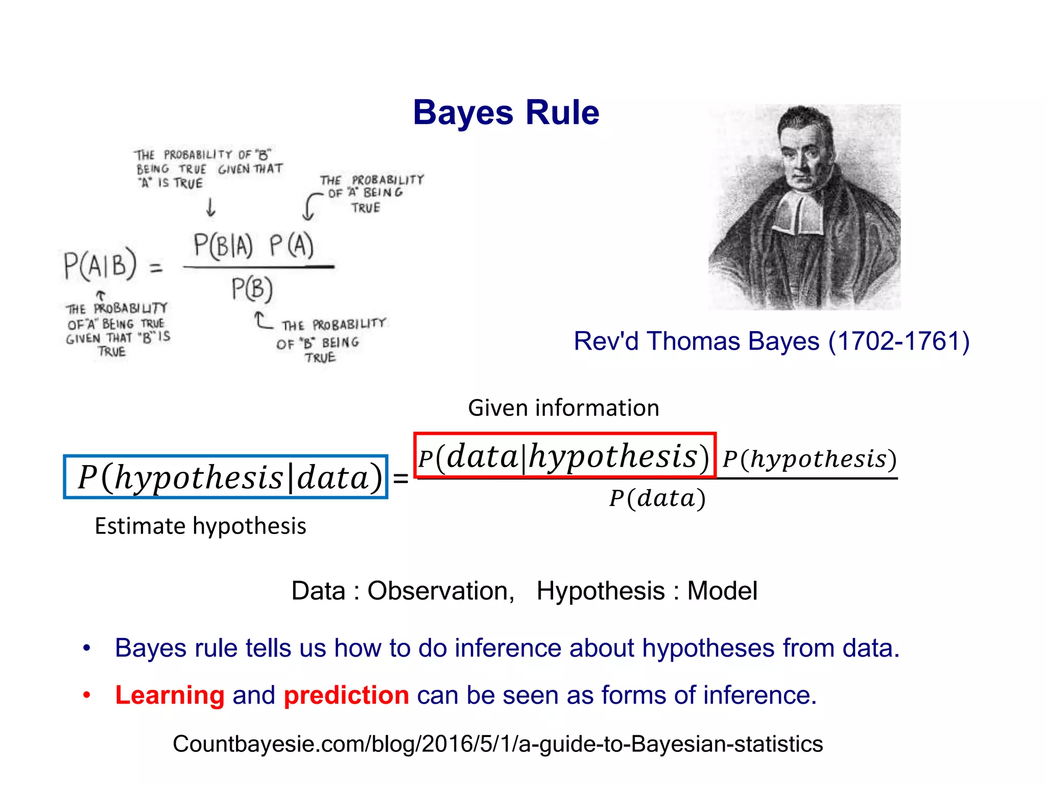
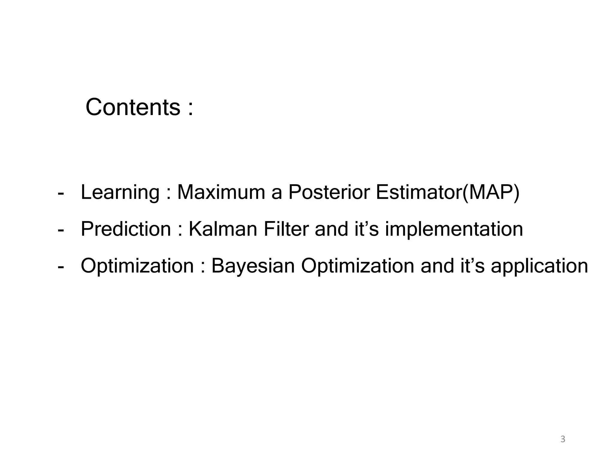
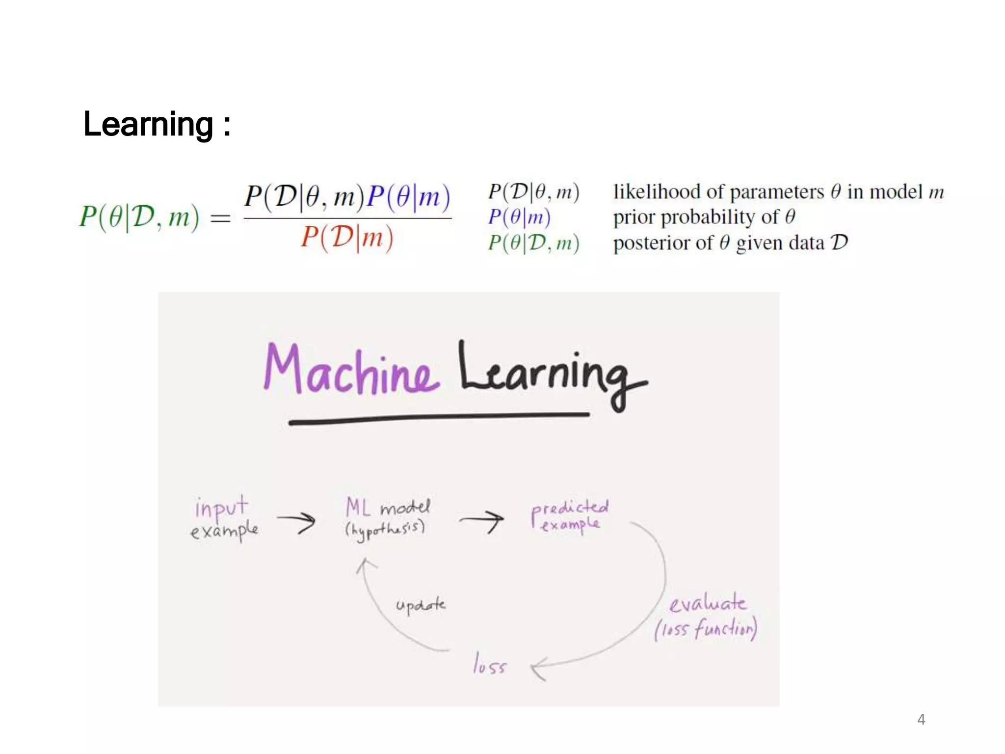
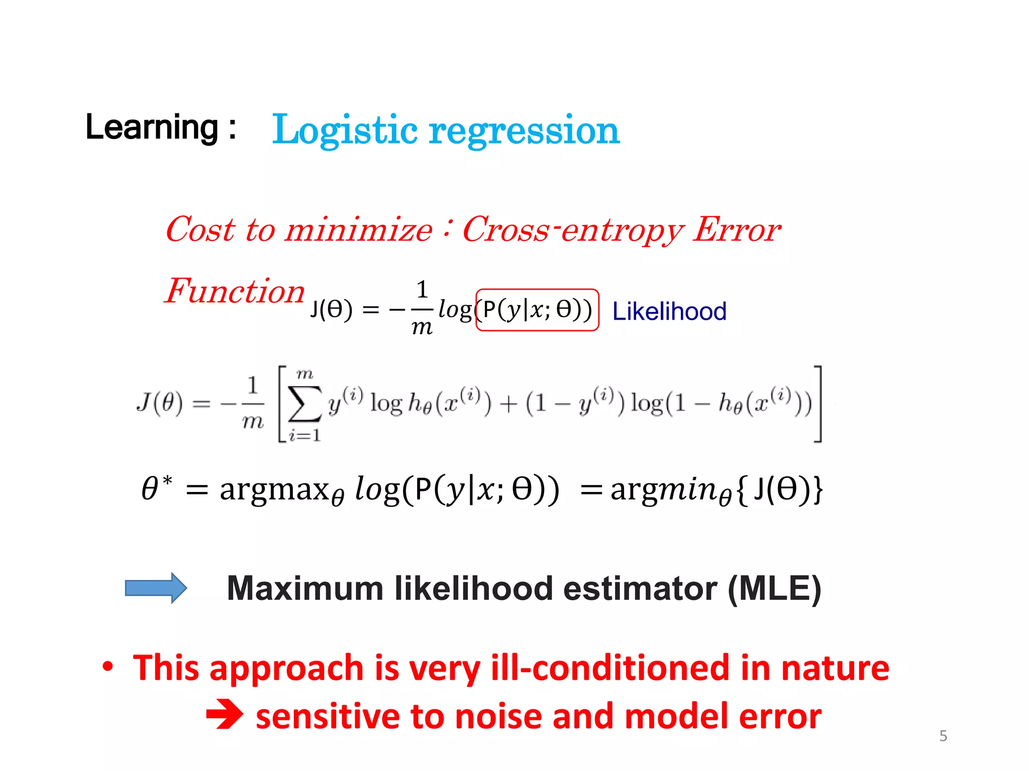
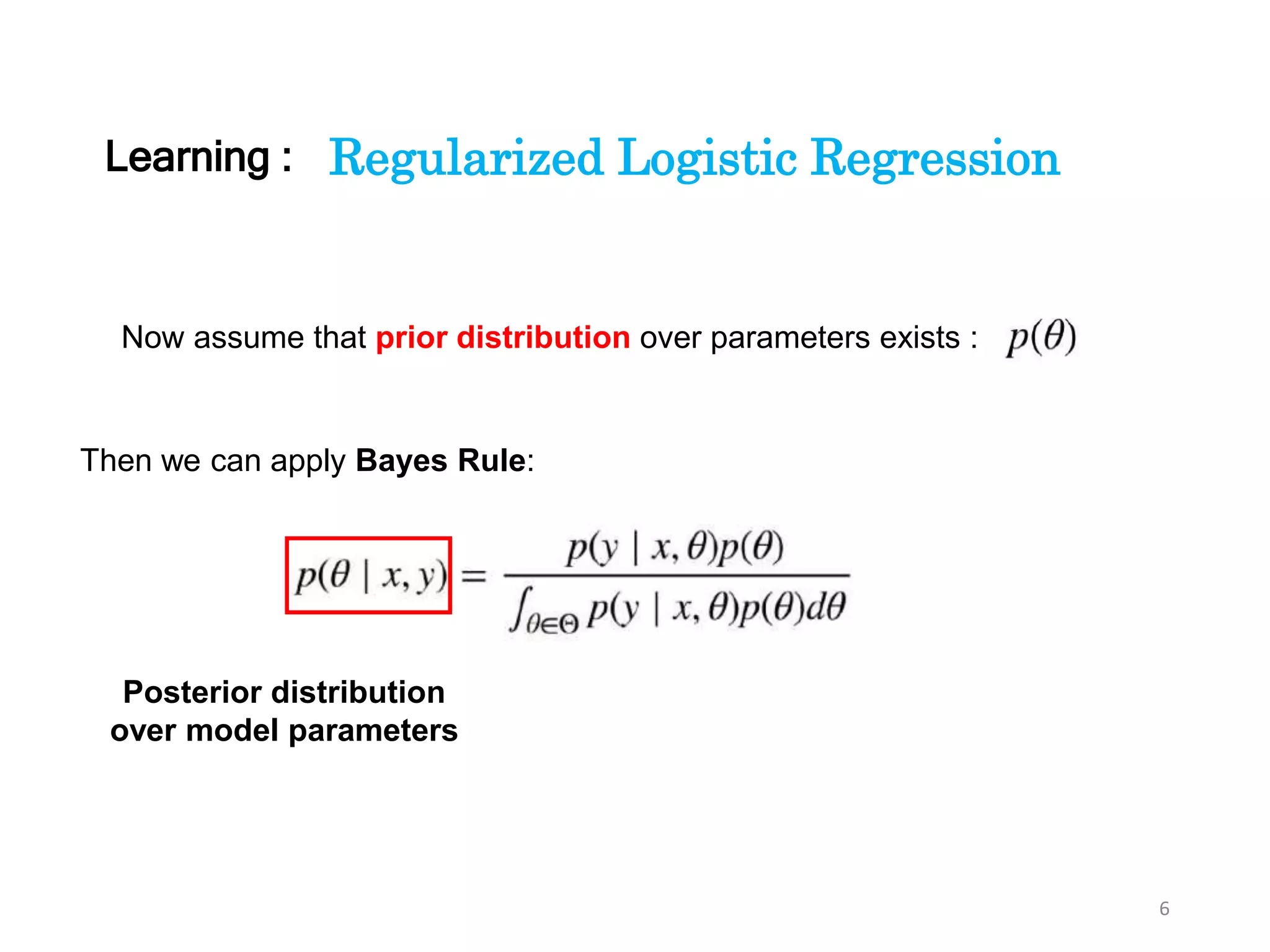
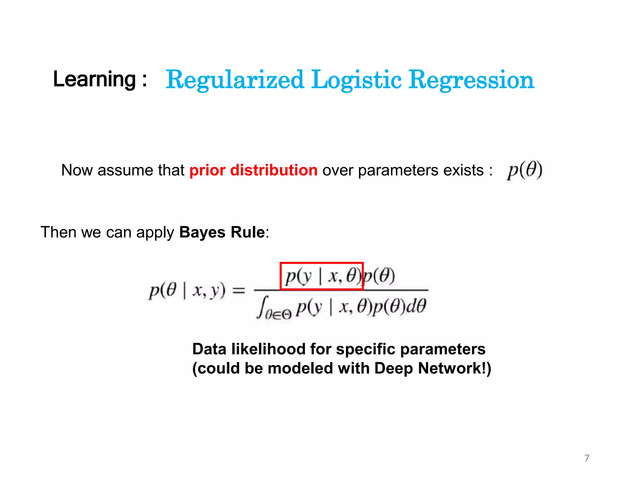
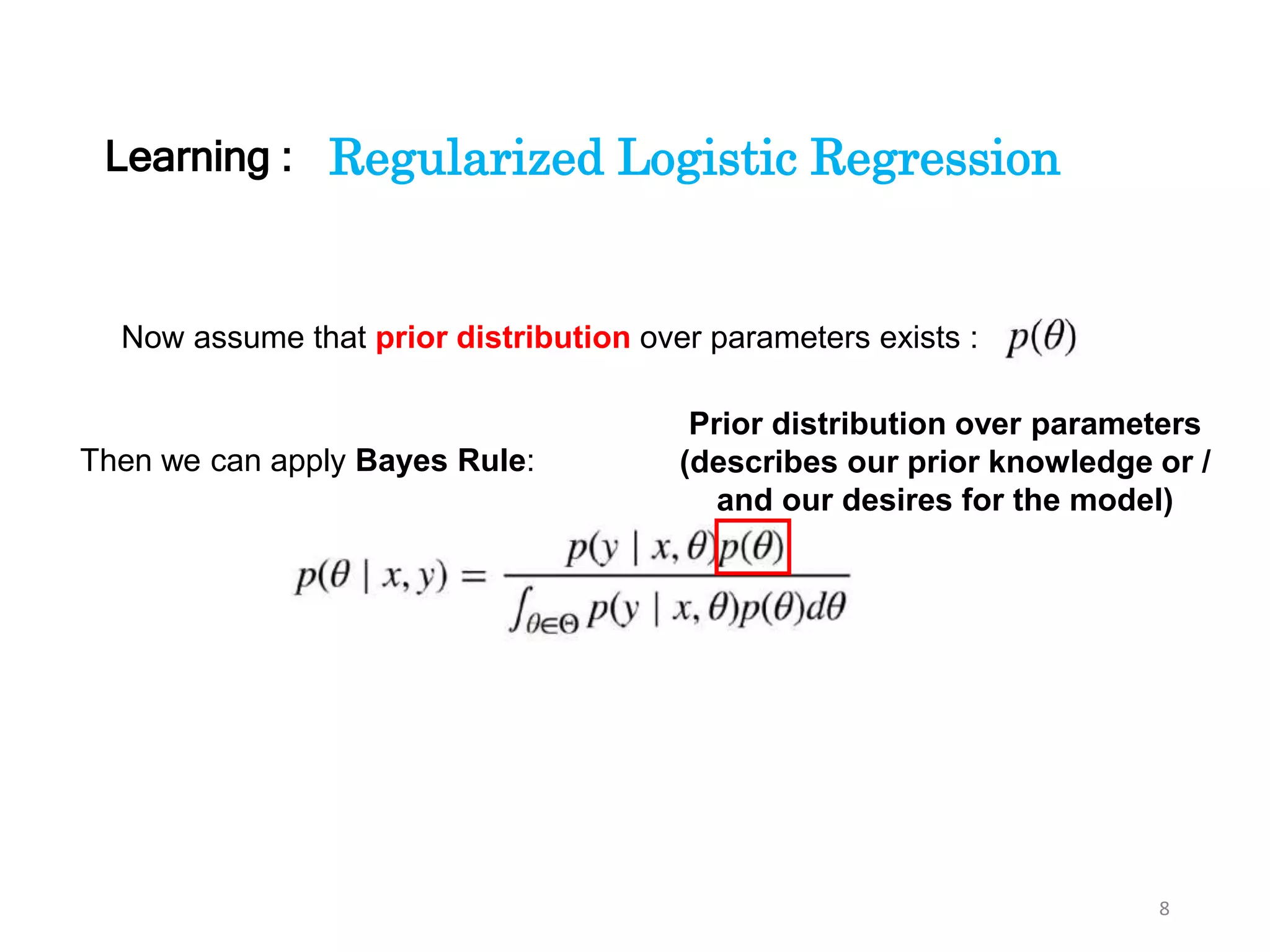
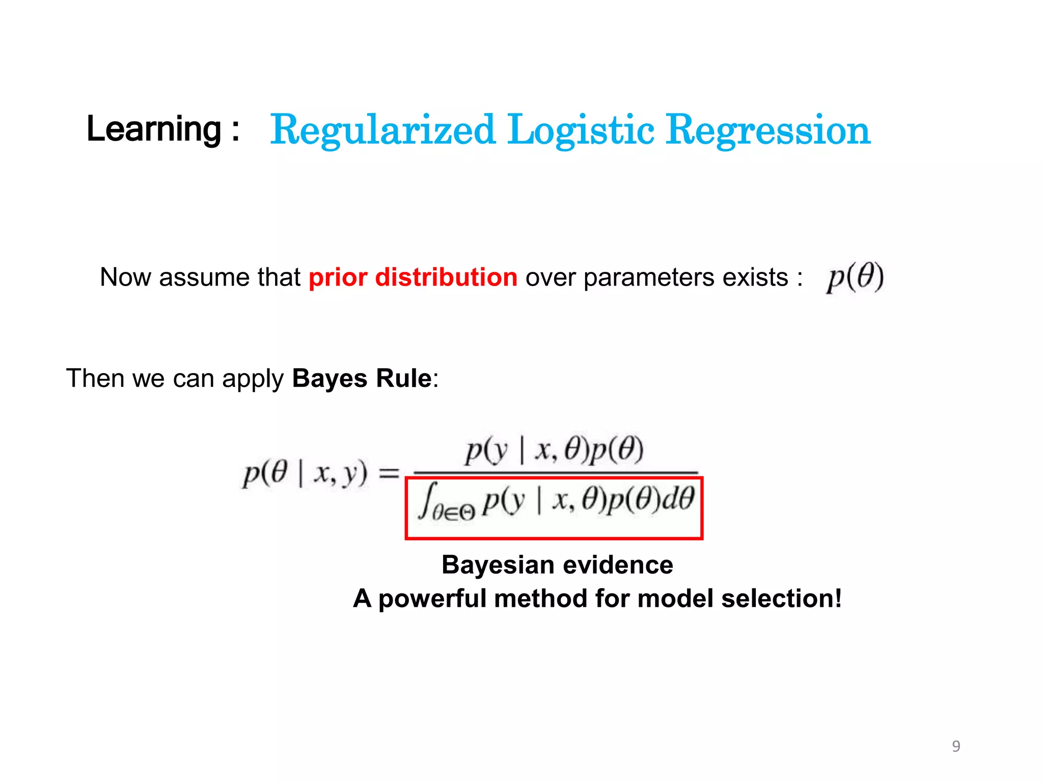
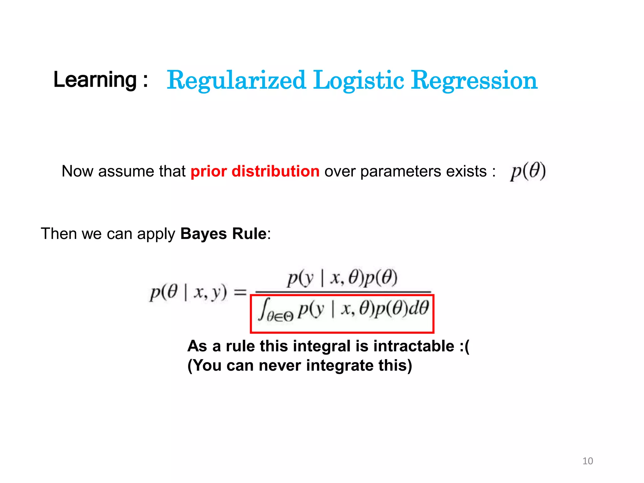
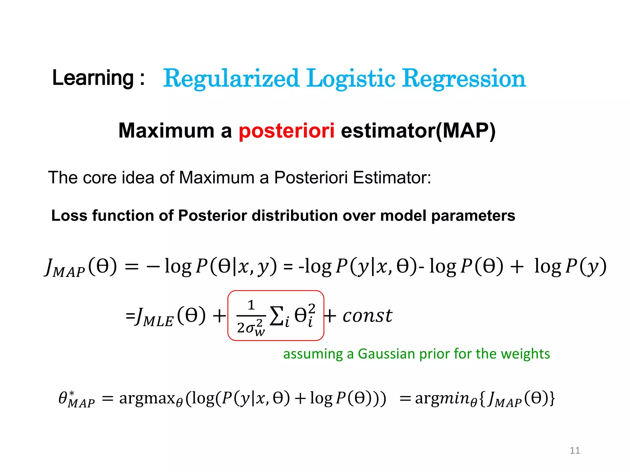
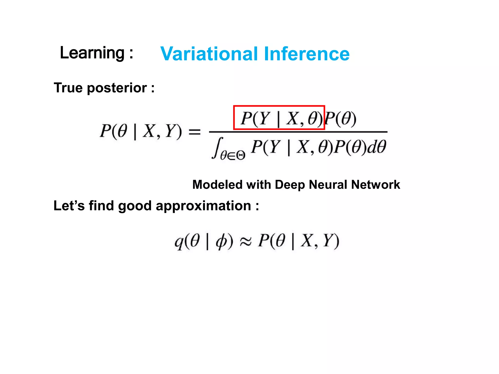
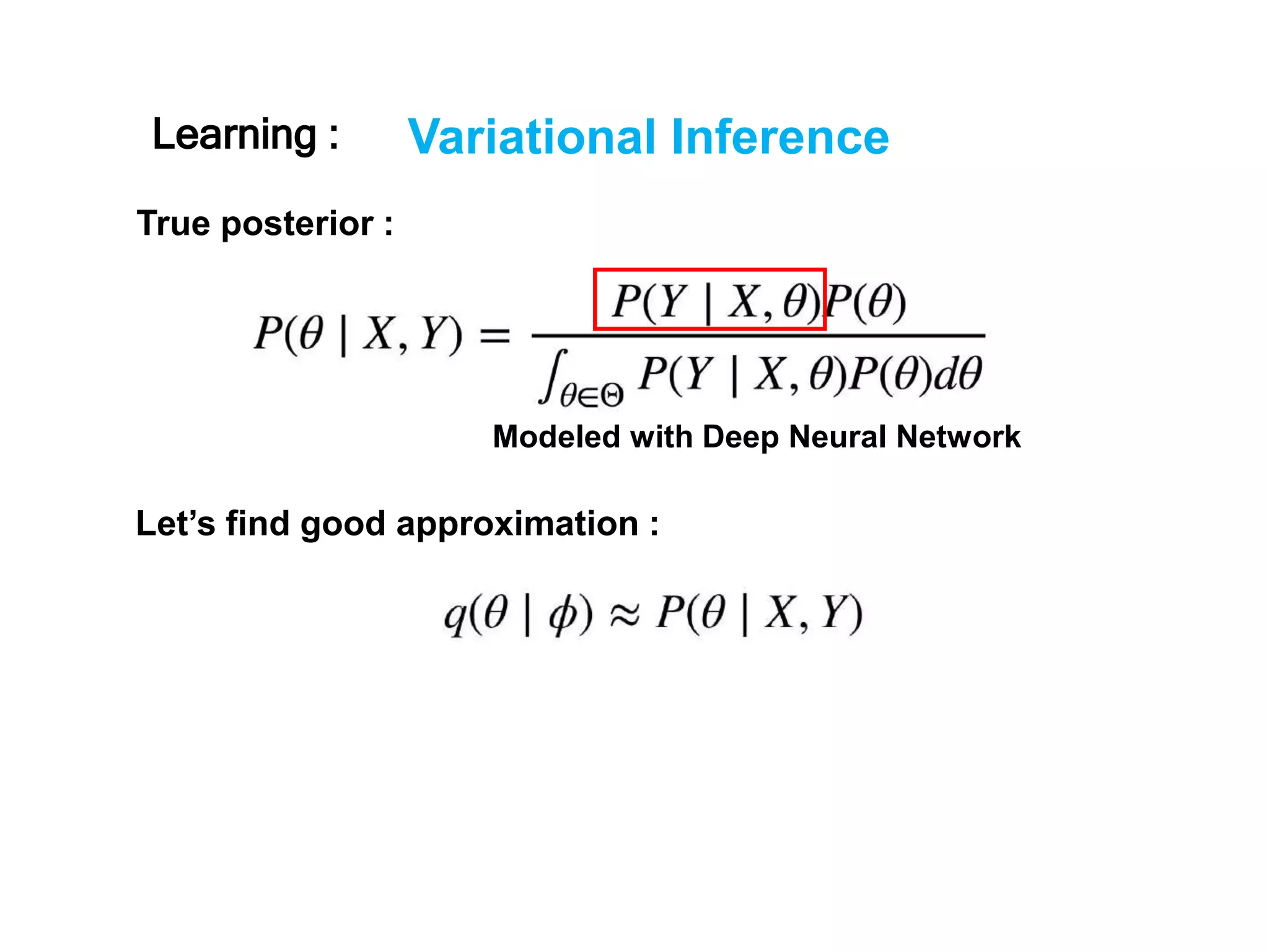
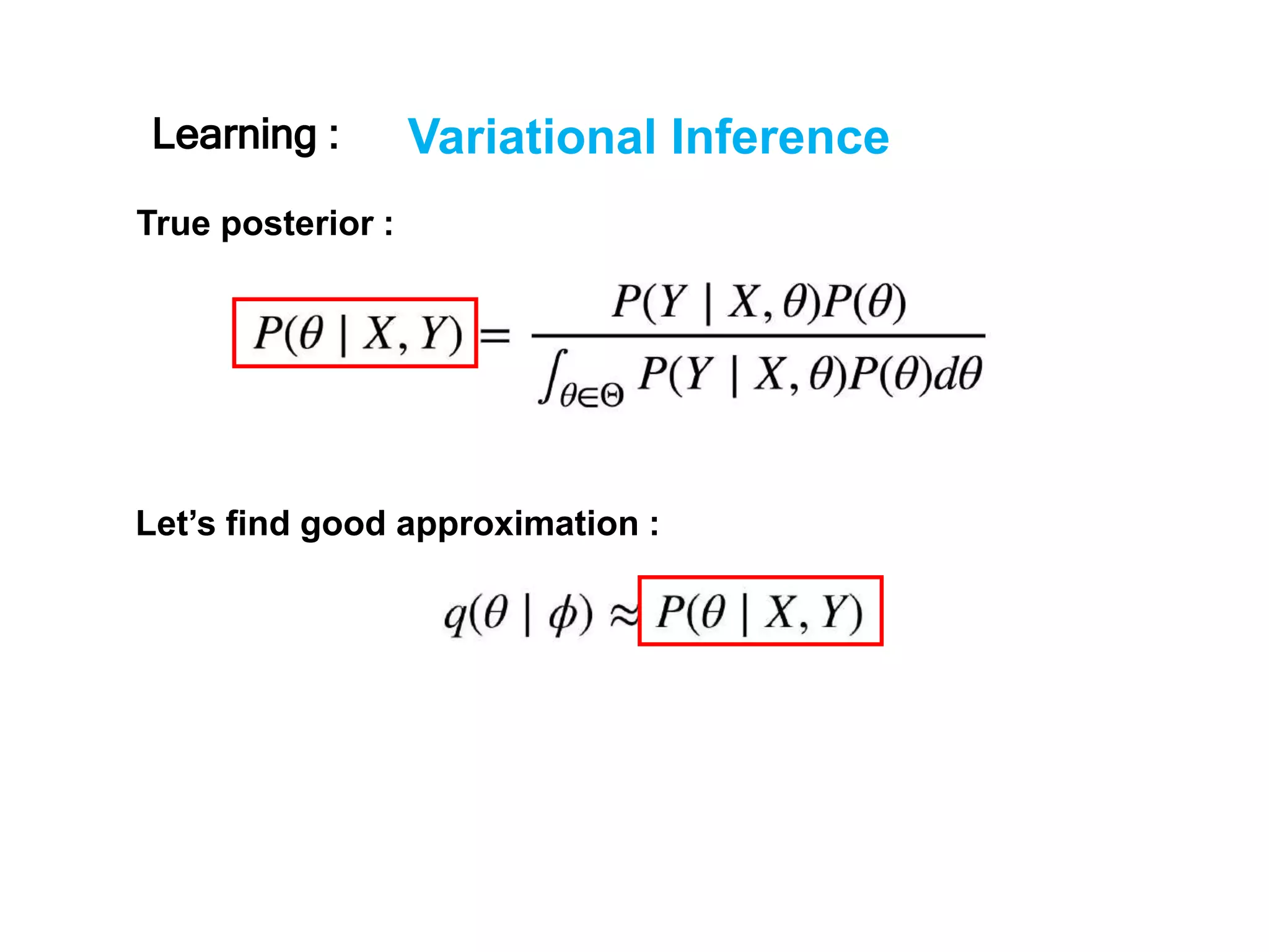
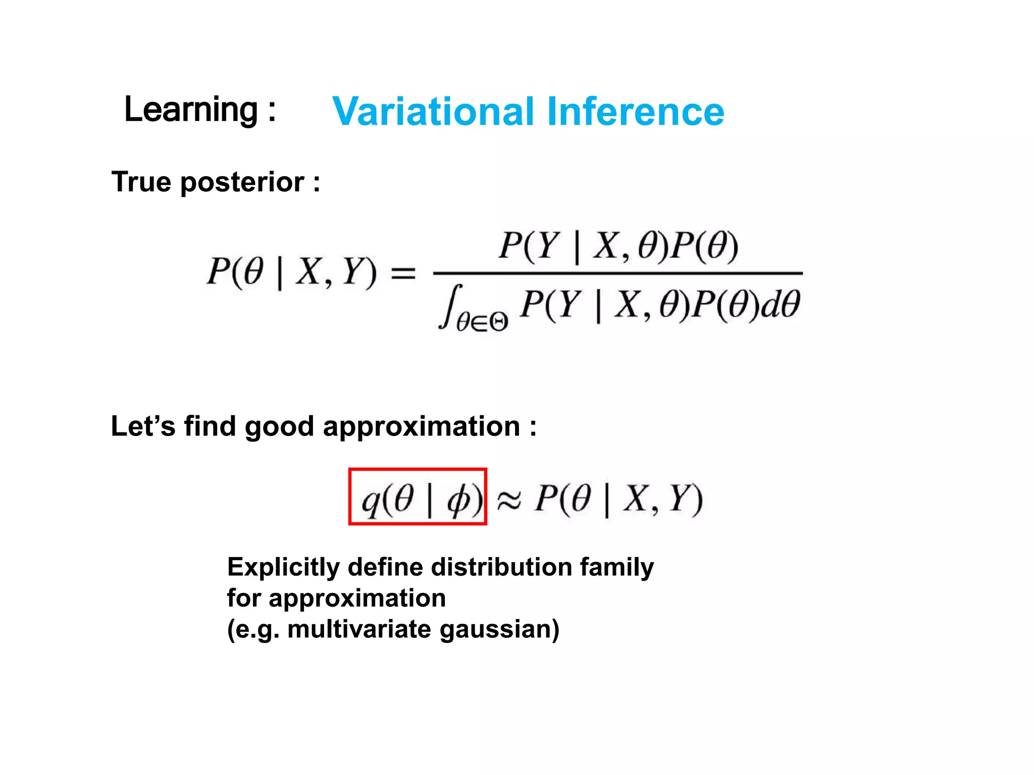
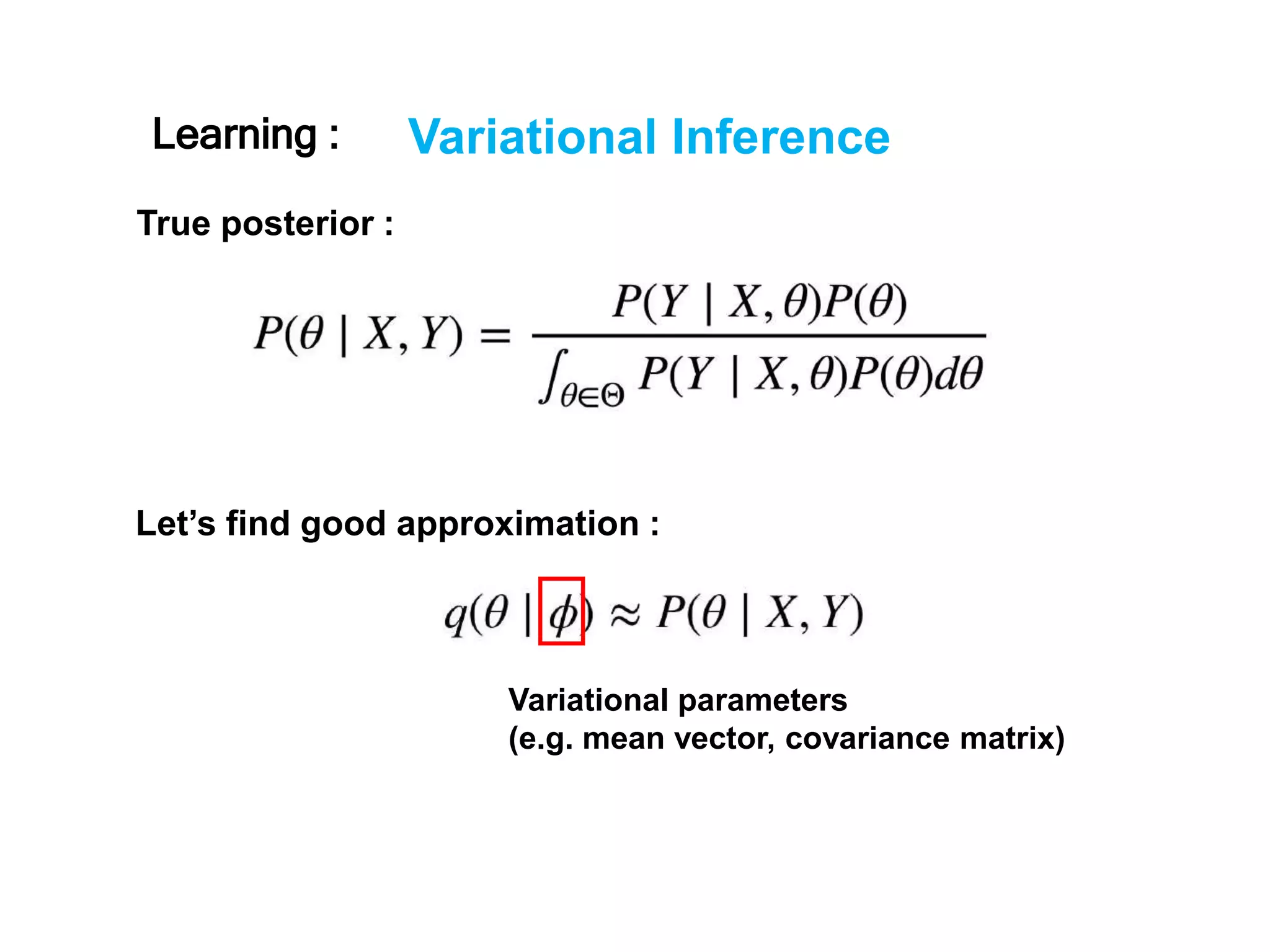
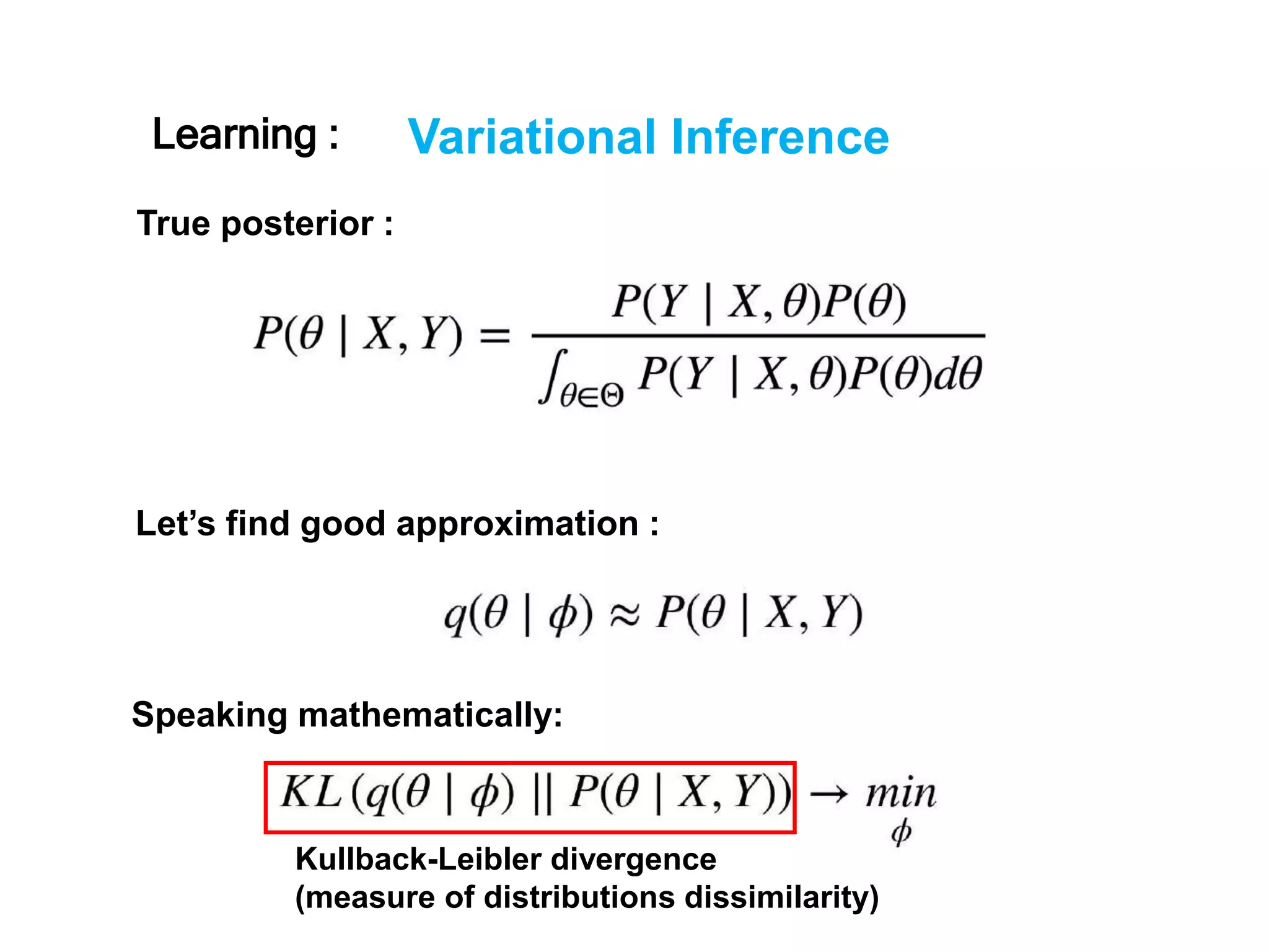
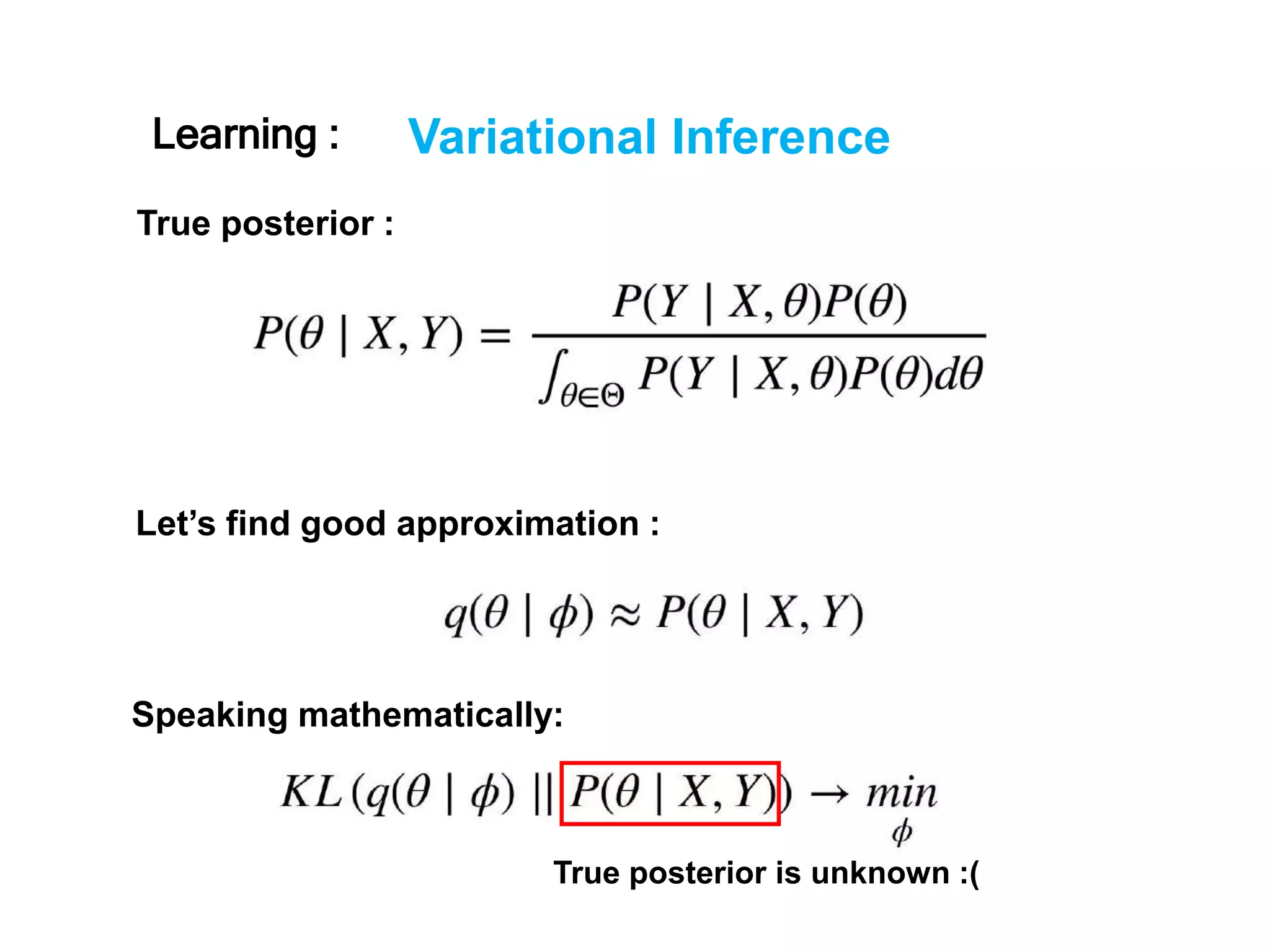
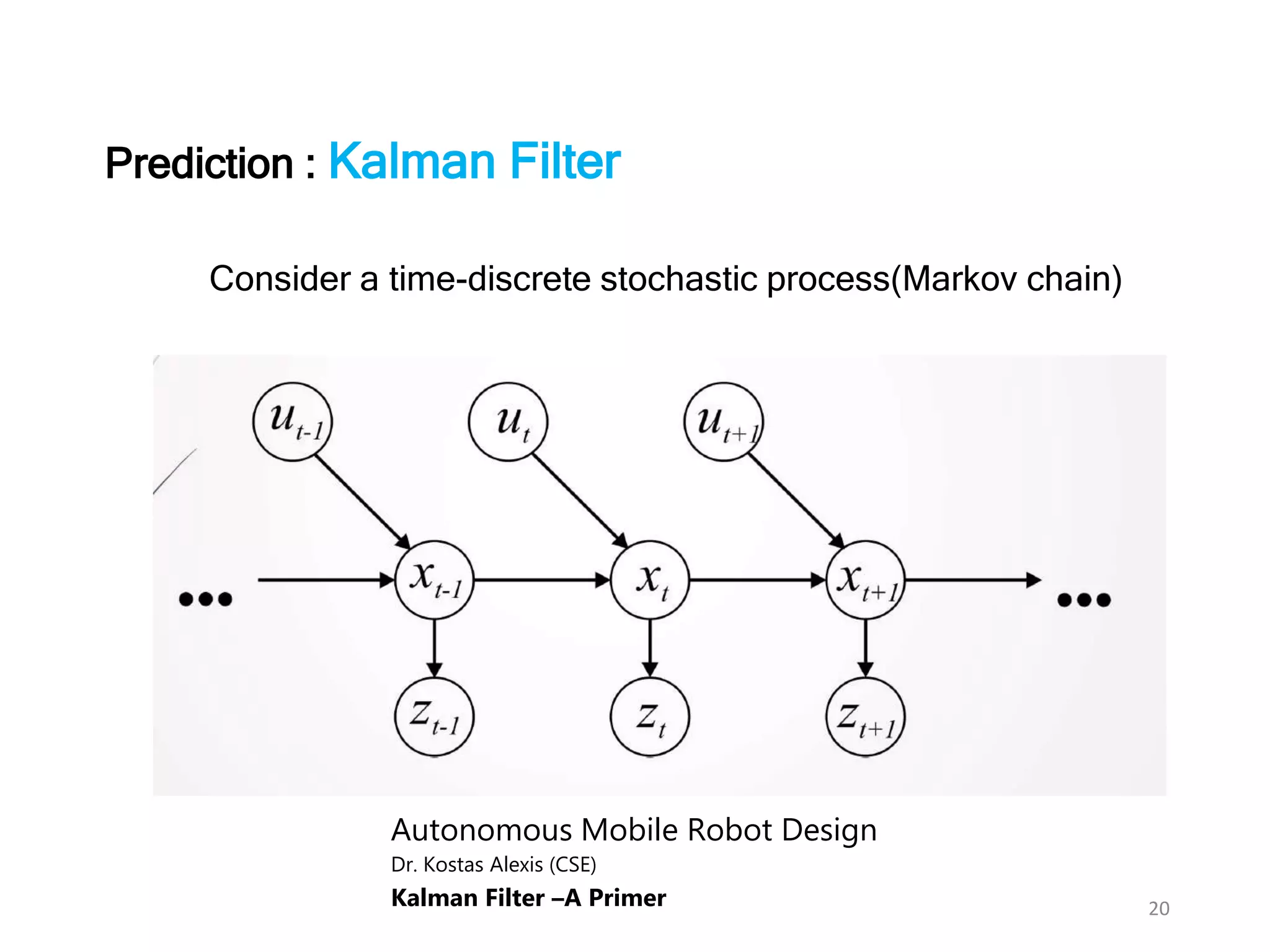
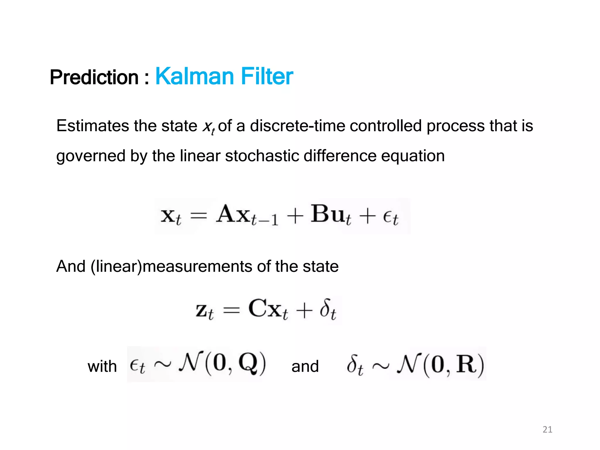
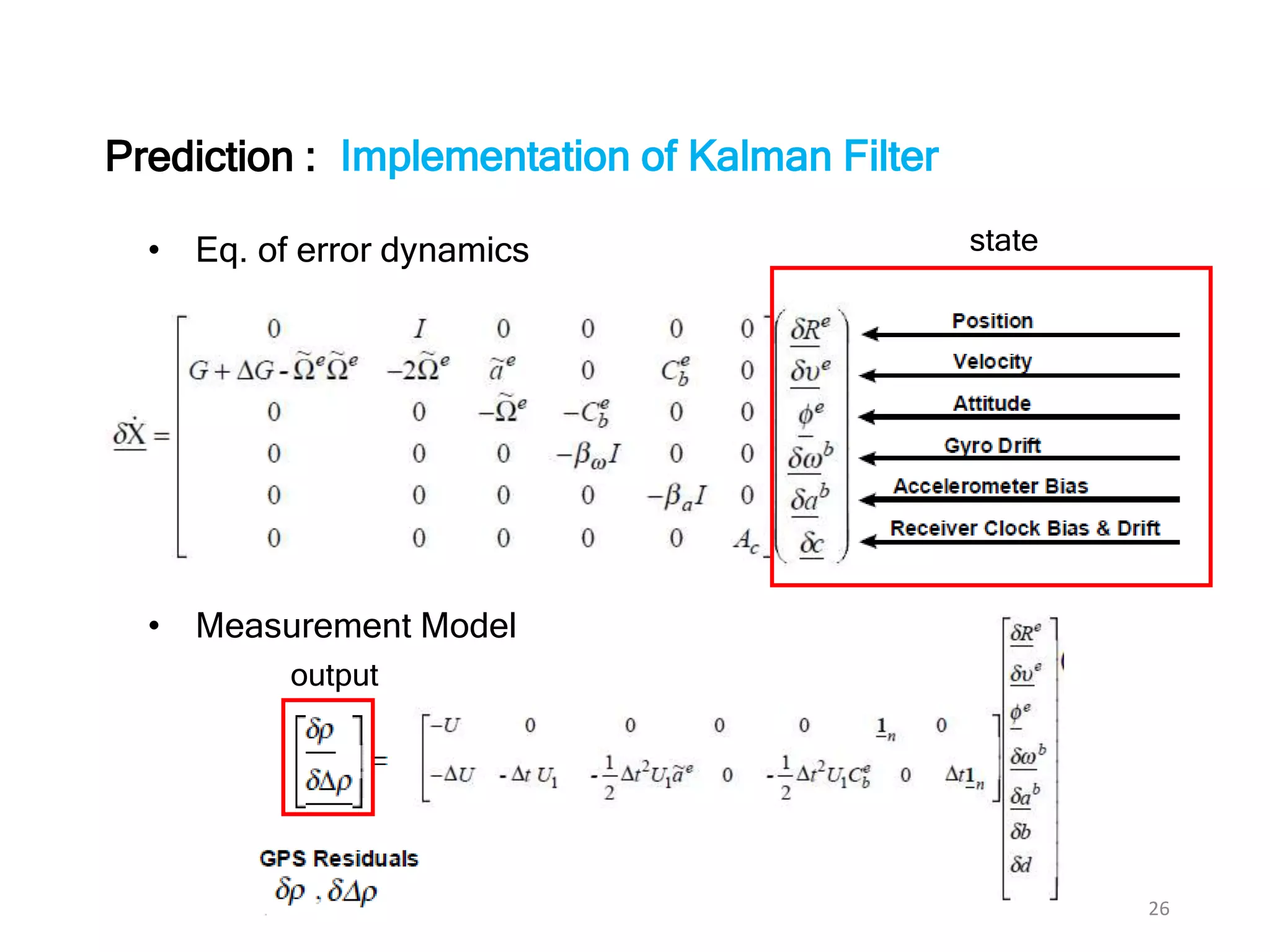
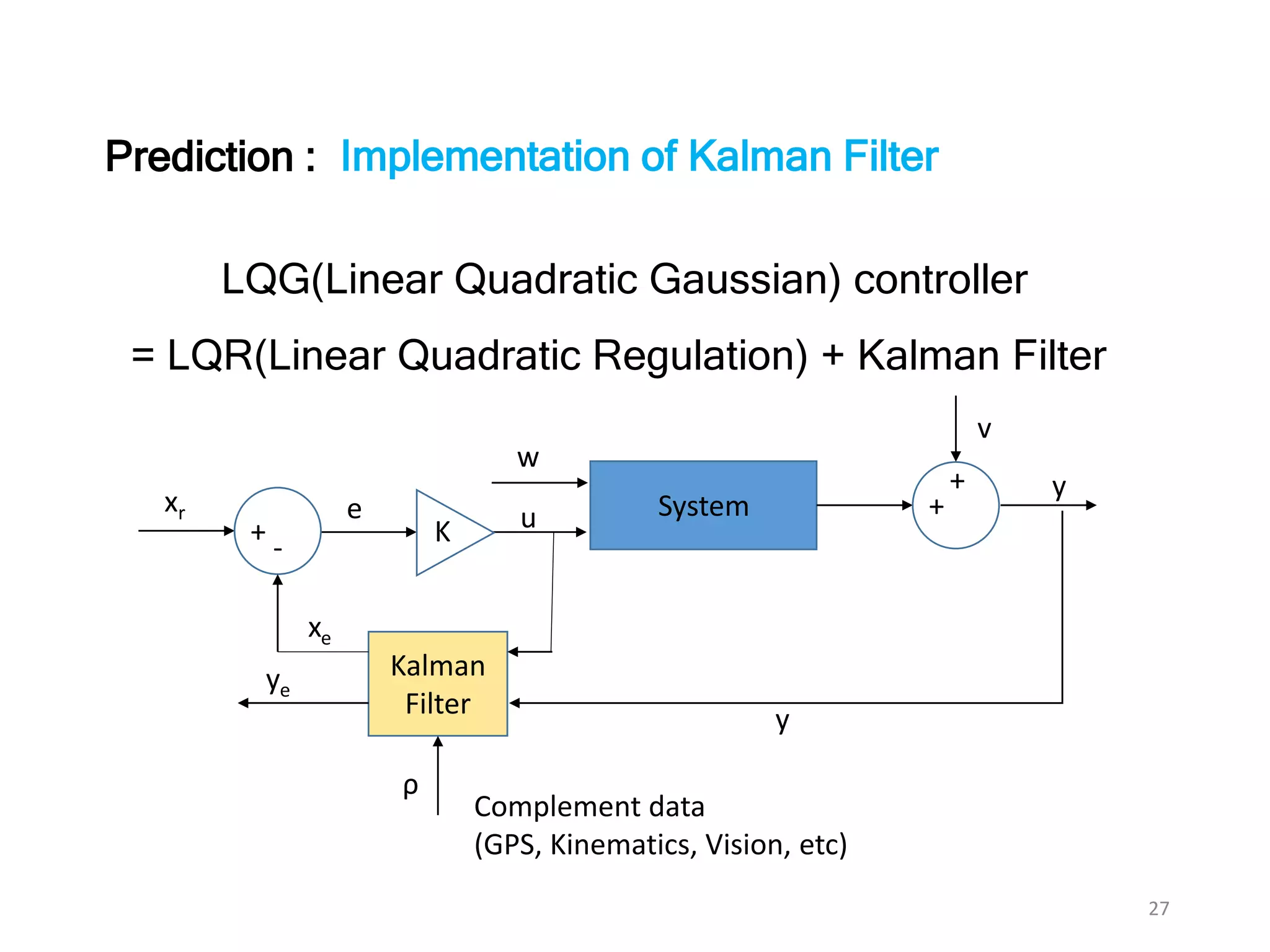
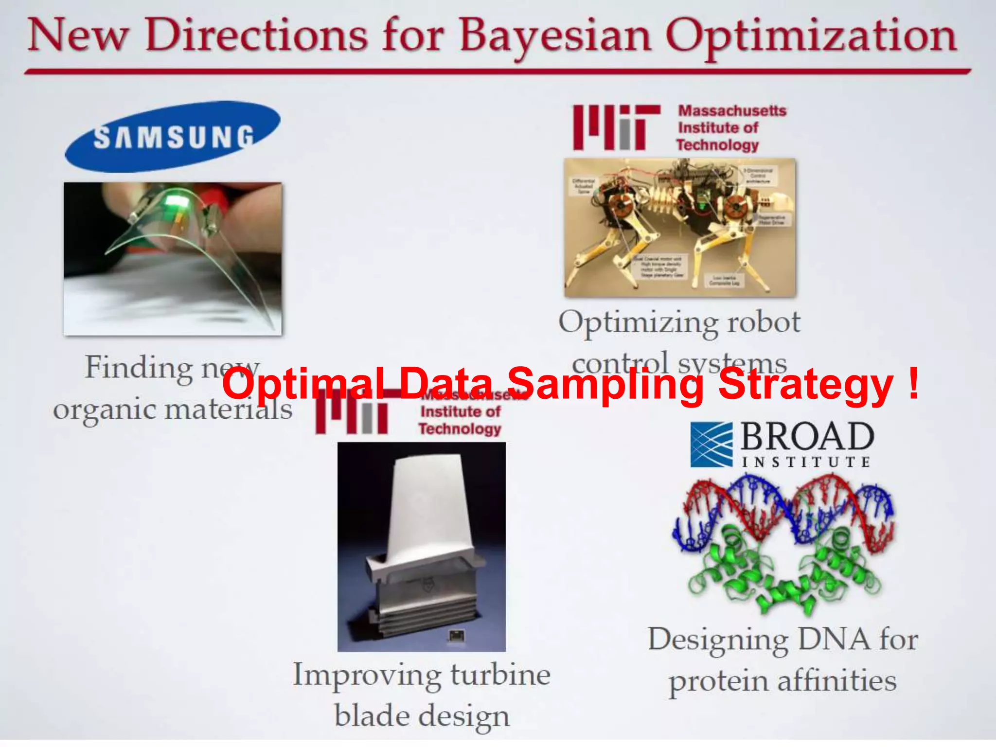
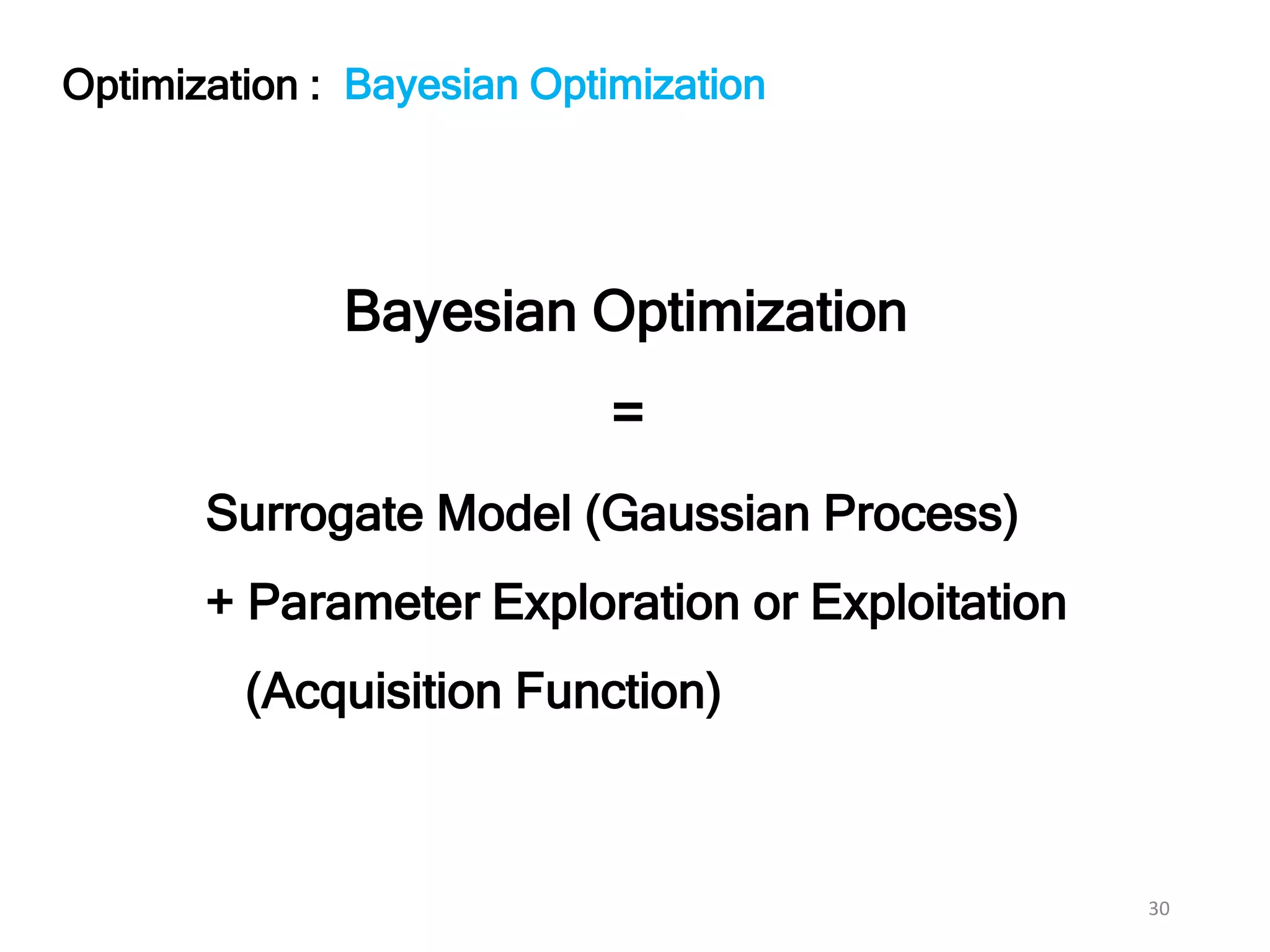
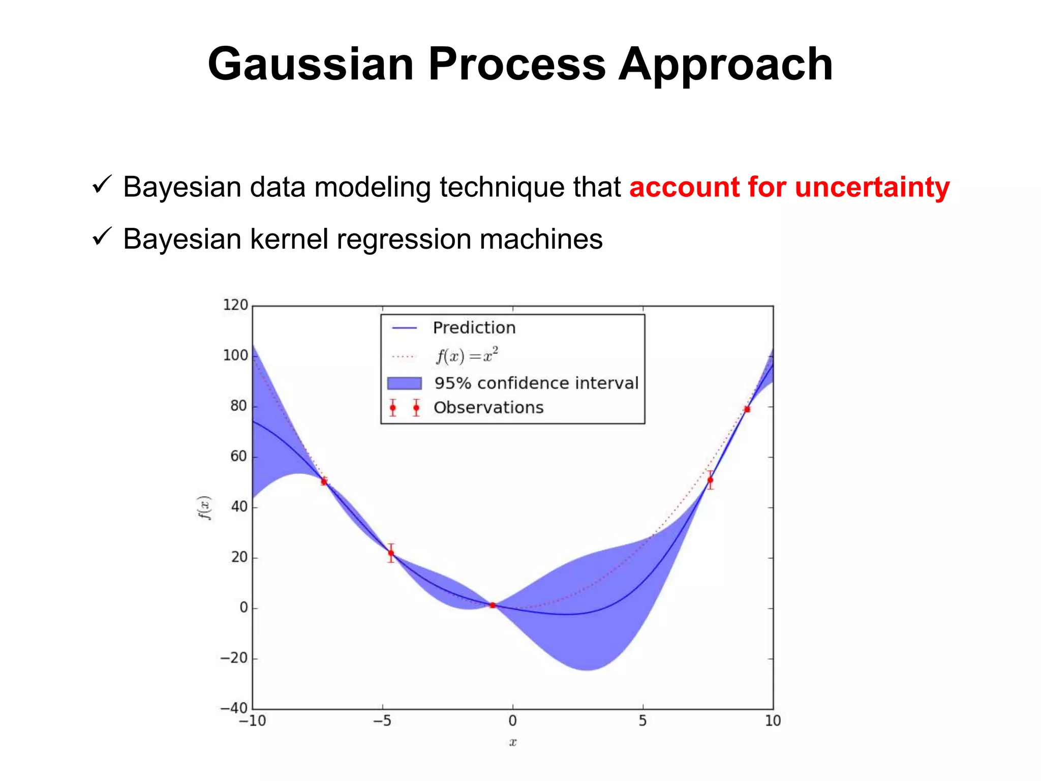
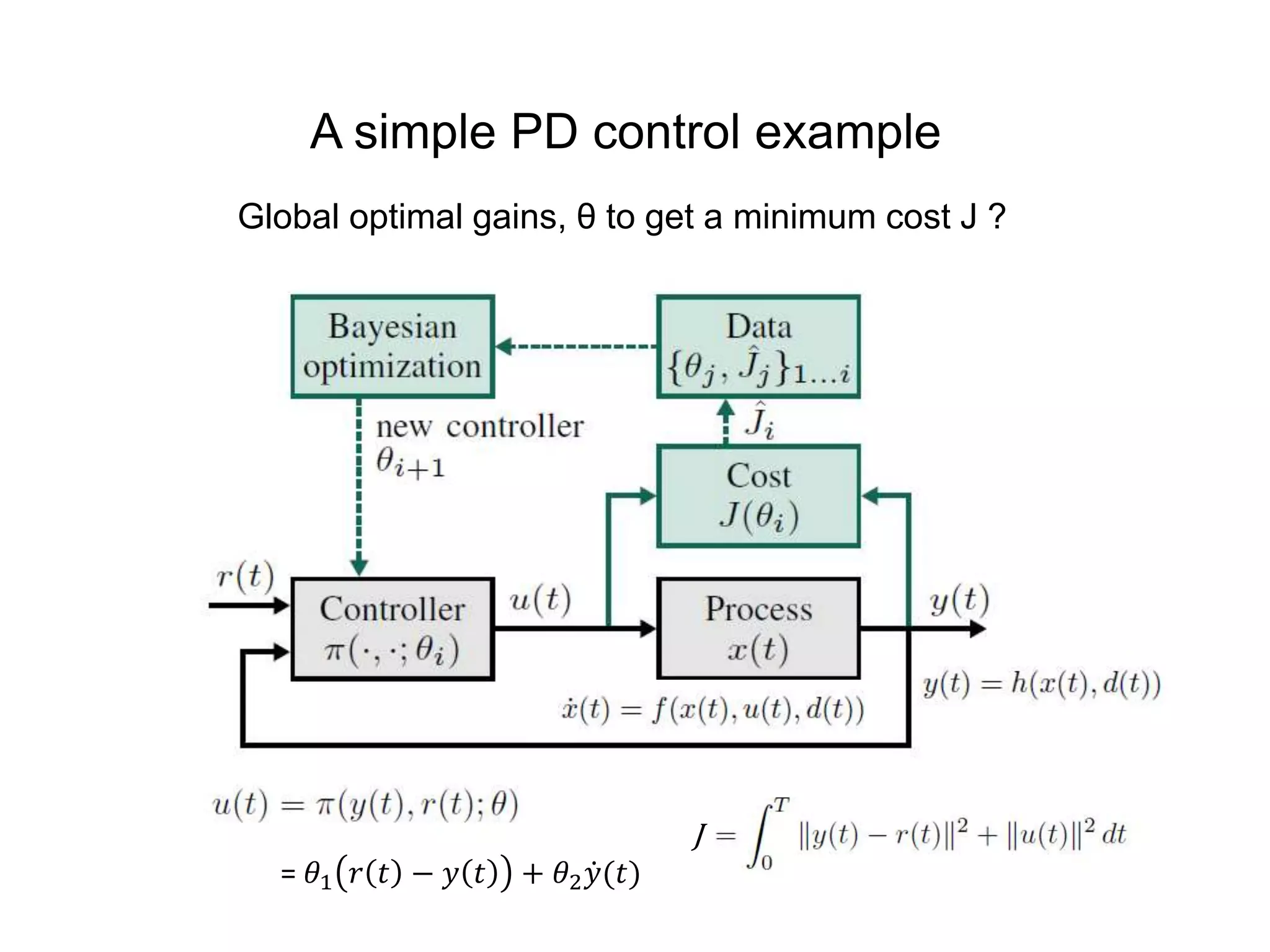
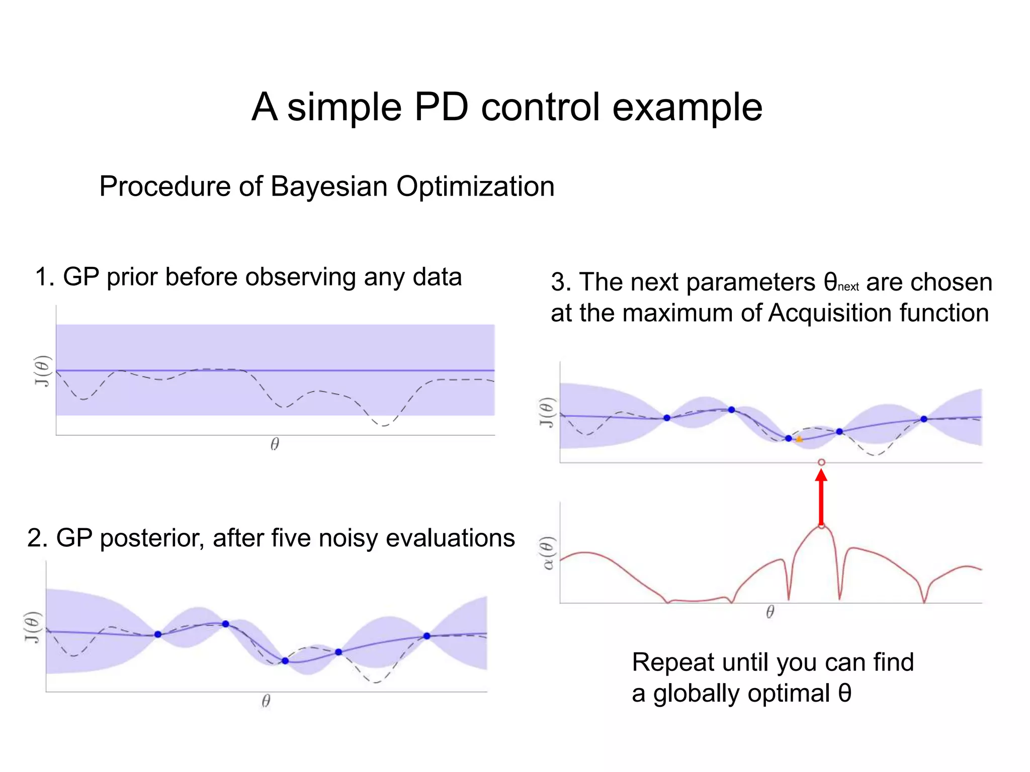
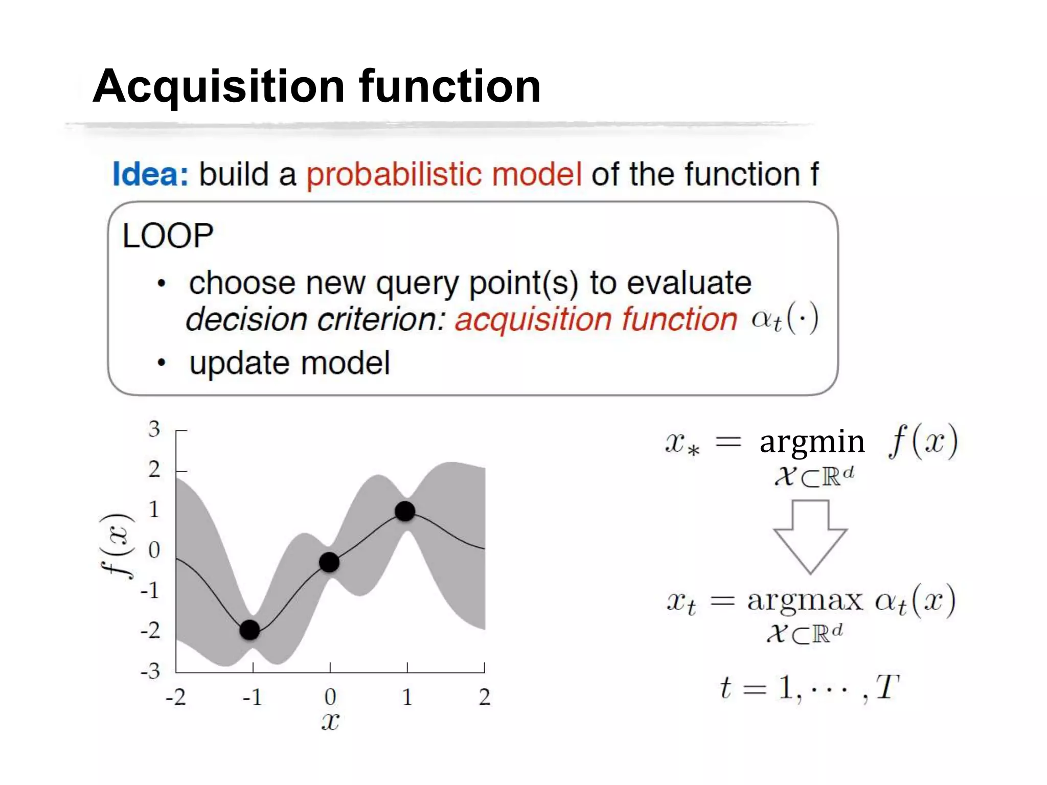
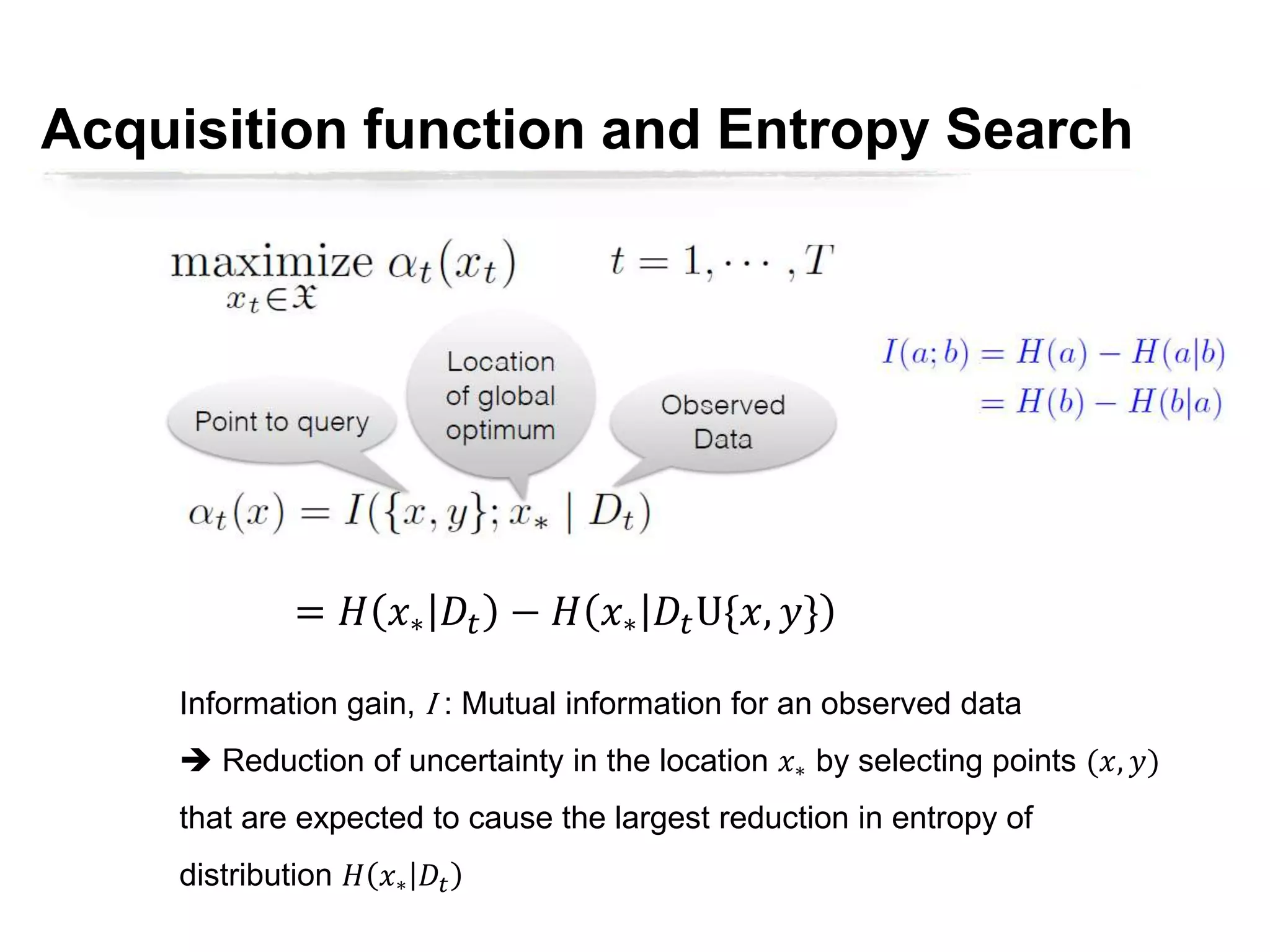
The document discusses Bayesian inference, focusing on learning, prediction, and optimization, with a particular emphasis on tools like the Kalman filter and Bayesian optimization techniques. It covers concepts such as maximum a posteriori estimation, regularized logistic regression, and Gaussian processes for modeling uncertainty in data. Additionally, it outlines the algorithmic implementations and methodologies for applying these Bayesian techniques in various settings.

1. Bayesian Inference :
Kalman filter에서 Optimization까지

2. Bayes Rule
𝑃 ℎ𝑦𝑝𝑜𝑡ℎ𝑒𝑠𝑖𝑠 𝑑𝑎𝑡𝑎 =
𝑃 𝑑𝑎𝑡𝑎 ℎ𝑦𝑝𝑜𝑡ℎ𝑒𝑠𝑖𝑠 𝑃(ℎ𝑦𝑝𝑜𝑡ℎ𝑒𝑠𝑖𝑠)
𝑃(𝑑𝑎𝑡𝑎)
• Bayes rule tells us how to do inference about hypotheses from data.
• Learning and prediction can be seen as forms of inference.
Given information
Estimate hypothesis
Rev'd Thomas Bayes (1702-1761)
Data : Observation, Hypothesis : Model
Countbayesie.com/blog/2016/5/1/a-guide-to-Bayesian-statistics

3. 3
Contents :
- Learning : Maximum a Posterior Estimator(MAP)
- Prediction : Kalman Filter and it’s implementation
- Optimization : Bayesian Optimization and it’s application

4. 4
Learning :

5. 5
Cost to minimize : Cross-entropy Error
Function J(ϴ) = −
1
𝑚
𝑙𝑜g(P 𝑦 𝑥; ϴ )
Logistic regression
Likelihood
Maximum likelihood estimator (MLE)
𝜃∗ = argmax 𝜃 𝑙𝑜g(P 𝑦 𝑥; ϴ ) = arg𝑚𝑖𝑛 𝜃{ J(ϴ)}
• This approach is very ill-conditioned in nature
 sensitive to noise and model error
Learning :

6. 6
Regularized Logistic Regression
Now assume that prior distribution over parameters exists :
Then we can apply Bayes Rule:
Posterior distribution
over model parameters
Learning :

7. 7
Regularized Logistic Regression
Now assume that prior distribution over parameters exists :
Then we can apply Bayes Rule:
Data likelihood for specific parameters
(could be modeled with Deep Network!)
Learning :

8. 8
Regularized Logistic Regression
Now assume that prior distribution over parameters exists :
Then we can apply Bayes Rule:
Prior distribution over parameters
(describes our prior knowledge or /
and our desires for the model)
Learning :

9. 9
Regularized Logistic Regression
Now assume that prior distribution over parameters exists :
Then we can apply Bayes Rule:
Bayesian evidence
A powerful method for model selection!
Learning :

10. 10
Regularized Logistic Regression
Now assume that prior distribution over parameters exists :
Then we can apply Bayes Rule:
Learning :
As a rule this integral is intractable :(
(You can never integrate this)

11. 11
The core idea of Maximum a Posteriori Estimator:
Maximum a posteriori estimator(MAP)
𝐽 𝑀𝐴𝑃 ϴ = − log 𝑃 ϴ 𝑥, 𝑦 = -log 𝑃 𝑦 𝑥, ϴ - log 𝑃 ϴ + log 𝑃 𝑦
=𝐽 𝑀𝐿𝐸 ϴ +
1
2𝜎 𝑤
2 𝑖 ϴ𝑖
2
+ 𝑐𝑜𝑛𝑠𝑡
𝜃 𝑀𝐴𝑃
∗
= argmax 𝜃(log(𝑃 𝑦 𝑥, ϴ + log 𝑃 ϴ )) = arg𝑚𝑖𝑛 𝜃{ 𝐽 𝑀𝐴𝑃 ϴ }
Loss function of Posterior distribution over model parameters
assuming a Gaussian prior for the weights
Regularized Logistic RegressionLearning :

12. Variational Inference
True posterior :
Modeled with Deep Neural Network
Let’s find good approximation :
Learning :

13. Variational Inference
True posterior :
Modeled with Deep Neural Network
Let’s find good approximation :
Learning :

14. Variational Inference
True posterior :
Let’s find good approximation :
Learning :
Intractable integral :(

15. Variational Inference
True posterior :
Let’s find good approximation :
Learning :

16. Variational Inference
True posterior :
Let’s find good approximation :
Explicitly define distribution family
for approximation
(e.g. multivariate gaussian)
Learning :

17. Variational Inference
True posterior :
Let’s find good approximation :
Learning :
Variational parameters
(e.g. mean vector, covariance matrix)

18. Variational Inference
True posterior :
Let’s find good approximation :
Kullback-Leibler divergence
(measure of distributions dissimilarity)
Learning :
Speaking mathematically:

19. Variational Inference
True posterior :
Let’s find good approximation :
Speaking mathematically:
True posterior is unknown :(
Learning :

20. 20
Prediction : Kalman Filter
Autonomous Mobile Robot Design
Dr. Kostas Alexis (CSE)
Kalman Filter –A Primer
Consider a time-discrete stochastic process(Markov chain)

21. 21
Estimates the state xt of a discrete-time controlled process that is
governed by the linear stochastic difference equation
And (linear)measurements of the state
with and
Prediction : Kalman Filter

22. 22
Bayes Filter Algorithm
For each step, do:
• Apply motion model
• Apply to sensor model
constant
Prediction :

23. 23
From Bayes Filter to Kalman Filter
For each step, do:
• Apply motion model
• Apply to sensor model
Prediction :

24. 24
Kalman Filter AlgorithmPrediction :
Kt : Kalman Gain
Cov. of state Cov. of measurement noise
>>∽1 for
<<∽0 for
While passing through tunnel

25. 25
Implementation of Kalman FilterPrediction :
GPS aided IMU :
- Gyro has drift, bias, and alignment error
- GPS, vision or kinematics can cope with these inherent problems
“ASSESSMENT OF INTEGRATED GPS/INS FOR THE EX-171 EXTENDED
RANGE GUIDED MUNITION”, AIAA-98-4416

26. 26
• Eq. of error dynamics
Implementation of Kalman FilterPrediction :
• Measurement Model
state
output

27. 27
System
v
+
+ y
+
-
K
y
K
w
u
Kalman
Filter
xe
ye
xr e
Complement data
(GPS, Kinematics, Vision, etc)
ρ
Implementation of Kalman FilterPrediction :
LQG(Linear Quadratic Gaussian) controller
= LQR(Linear Quadratic Regulation) + Kalman Filter

28. 28
Implementation of Kalman FilterPrediction :

29. Optimal Data Sampling Strategy !

30. 30
Bayesian OptimizationOptimization :
Surrogate Model (Gaussian Process)
+ Parameter Exploration or Exploitation
(Acquisition Function)
Bayesian Optimization
=

31. Automatic Gain Tuning
based on
Gaussian Process Global Optimization
(= Bayesian Optimization)

32. 32
Bayesian OptimizationOptimization :

33. Short Introduction on
Gaussian Processes
Regression, Classification & Optimization

34. Why GPs ? :
- Provide Closed-Form Predictions !
- Effective for small data problems
- And Explainable !

35. How Do We Deal With Many Parameters, Little Data ?
1. Regularization
e.g., smoothing, L1 penalty, drop out in neural nets, large K
for K-nearest neighbor
2. Standard Bayesian approach
specify probability of data given weights, P(D|W)
specify weight priors given hyper-parameter α, P(W|α)
find posterior over weights given data, P(W|D, α)
With little data, strong weight prior constrains inference
3. Gaussian processes
place a prior over functions, p(f) directly rather than
over model parameters, p(w)

36. Functions : Relationship between Input and Output
Distribution of functions that satisfy
within the range of Input, X and Output, f
 Prior over functions, No Constraints
X
f
prior

37. • GP specifies a prior over functions, f(x)
• Suppose we have a set of observations:
• D = {(x1,y1), (x2, y2), (x3, y3), …, (xn,
yn)}
Standard Bayesian approach
• p(f|D) ~ p(D|f) p(f)
One view of Bayesian inference
• generating samples (the prior)
• discard all samples inconsistent with
our data, leaving the samples of
interest (the posterior)
• The Gaussian process allows us to
do this analytically.
Gaussian Process Approach
prior
posterior

38.  Bayesian data modeling technique that account for uncertainty
 Bayesian kernel regression machines
Gaussian Process Approach

39. Procedure to sample
2. Compute Covariance Matrix for a given 𝑋 = 𝑥1 … . 𝑥 𝑛
1. Let’s assume input, X and function, f distributed as follows
X
f

40. Procedure to sample
3. Compute SVD or Cholesky decomp. of K to get orthogonal basis
functions
K = 𝐴𝑆𝐵 𝑇 = 𝐿𝐿𝑇
4. Compute Basis Function
𝑓𝑖 = 𝐴𝑆1/2 𝑢𝑖
or 𝑓𝑖 = 𝐿𝑢𝑖
𝑢𝑖 ∶ 𝑟𝑎𝑛𝑑𝑜𝑚 𝑣𝑒𝑐𝑡𝑜𝑟 𝑤𝑖𝑡ℎ
𝑧𝑒𝑟𝑜 𝑚𝑒𝑎𝑛 𝑎𝑛𝑑 𝑢𝑛𝑖𝑡 𝑣𝑎𝑟𝑖𝑎𝑛𝑐𝑒
L : Lower part of Cholesky
decomp. of K
X
f
posterior
X
f
prior

41. J
= 𝜃1 𝑟 𝑡 − 𝑦 𝑡 + 𝜃2 𝑦(𝑡)
A simple PD control example
Global optimal gains, θ to get a minimum cost J ?

42. A simple PD control example
Procedure of Bayesian Optimization
1. GP prior before observing any data
2. GP posterior, after five noisy evaluations
3. The next parameters θnext are chosen
at the maximum of Acquisition function
Repeat until you can find
a globally optimal θ

43. argmin
Acquisition function

44. = 𝐻 𝑥∗ 𝐷𝑡 − 𝐻 𝑥∗ 𝐷𝑡U{𝑥, 𝑦}
Information gain, I : Mutual information for an observed data
 Reduction of uncertainty in the location 𝑥∗ by selecting points (𝑥, 𝑦)
that are expected to cause the largest reduction in entropy of
distribution 𝐻 𝑥∗ 𝐷𝑡
Acquisition function and Entropy Search