DSP

1. 1
EC 726: Advanced Digital Signal Processing
Spring 2009
Lecture 8: Discrete Kalman Filtering
Lecturer: Dr. Maha Elsabrouty
Electrical and Electronics Engineering

2. 2
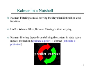
Kalman in a Nutshell
Kalman Filtering aims at solving the Bayesian Estimation cost
function.
Unlike Wiener Filter, Kalman filtering is time varying.
Kalman filtering depends on defining the system in state space
model: Prediction (estimate a priori) + correct (estimate a
posteriori)

3. 3
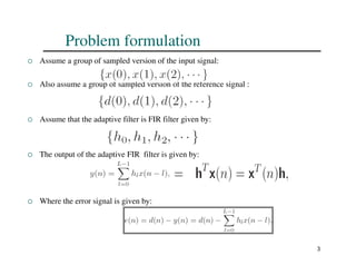
Problem formulation
Assume a group of sampled version of the input signal:
Also assume a group of sampled version of the reference signal :
Assume that the adaptive filter is FIR filter given by:
The output of the adaptive FIR filter is given by:
Where the error signal is given by:

4. 4
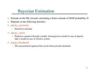
Bayesian Estimation
Extends on the ML towards calculating a better estimate of MAP probability ☺
Depends on the following densities:
p(yk|x1:k) posterior
Desired to calculate
p(yk|yk-1) prior
Predictive equation through a model, Autoregressive model in case of speech,
Jake’s model in case of wireless system.
p(xk|yk) likelihood
The measurement equation that can be observed and calculated.

5. 5
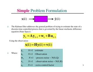
Simple Problem Formulation
The Kalman filter addresses the general problem of trying to estimate the state of a
discrete-time controlled process that is governed by the linear stochastic difference
equation (State Space):
Using the observation:
Where:
1
1 −
− +
+
= k
k
k
k u
B
w
y
A
y
)
(
)
(
)
( k
k
k v
y
H
x +
=
factor
control
e
:
1
R)
N(0,
~
noise
n
observatio
:
1
Q)
N(0,
~
noise
process
:
1
n
Observatio
:
1
estimate
:
1
xtra
N
u
N
N
N
N
k
k
k
k
k
×
×
×
×
×
v
w
x
y
)
(k
x )
(
ˆ k
y

6. 6
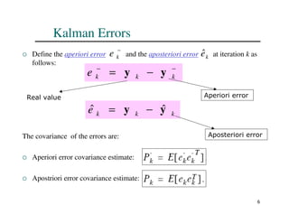
Kalman Errors
Define the aperiori error and the aposteriori error at iteration k as
follows:
The covariance of the errors are:
Aperiori error covariance estimate:
Apostriori error covariance estimate:
−
k
e k
ê
−
−
−
= k
k
k
e y
y
Real value Aperiori error
k
k
k
e y
y ˆ
ˆ −
=
Aposteriori error

7. 7
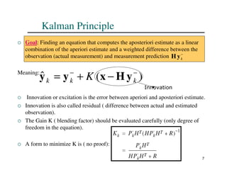
Kalman Principle
Goal: Finding an equation that computes the aposteriori estimate as a linear
combination of the aperiori estimate and a weighted difference between the
observation (actual measurement) and measurement prediction
Meaning:
Innovation or excitation is the error between aperiori and aposteriori estimate.
Innovation is also called residual ( difference between actual and estimated
observation).
The Gain K ( blending factor) should be evaluated carefully (only degree of
freedom in the equation).
A form to minimize K is ( no proof):
−
k
y
H
)
(
ˆ −
−
−
+
= k
k
k K y
H
x
y
y
Innovation

8. 8
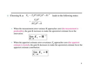
Choosing K as leads to the following notes:
When the measurement error variance R approaches zero (the measurement is
predictable), the gain K increases to make the apestoriori estimate favor the
innovation:
When the apperiori estimate error covariance approaches zero (the apperiori
estimate is trusted), the gain K decreases to make the apestoriori estimate favor the
apperiori estimate contribution:
1
lim −
→
= H
0
R
k
K
0
0
P
=
→
− k
K
k
lim

9. 9
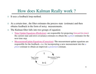
How does Kalman Really work ?
It uses a feedback loop method.
At a certain time , the filter estimates the process state (estimate) and then
obtains feedback in the form of noisy measurements.
The Kalman filter falls into two groups of equation:
Time Update Equations (Prediction): are responsible for projecting forward (in time)
the current state and error covariance estimates to obtain the a priori estimates for the
next time step.
MeasurementUpdate Equations (Correction): The measurement update equations are
responsible for the feedback—i.e. for incorporating a new measurement into the a
priori estimate to obtain an improved a posteriori estimate.
t
t+1

10. 10
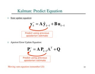
Kalman: Predict Equation
State update equation:
Aperiori Error Update Equation:
Moving sum equation (remember LS)
1
1
ˆ −
−
−
+
= k
k
k u
B
y
A
y
Q
P
A
P +
Α
= −
− T
k
k 1
Predict using previous
aposteriori estimate
Predict using previous
aposteriori estimate

11. 11
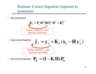
Kalman: Correct Equation (Aperiori to
posteriori)
Gain Calculation:
State Correct Equation:
Error Correct Equation:
( ) 1
−
−
−
+
= R
H
P
H
H
P
K T
k
T
k
k
Same instant k, use
aperiori estimate
)
(
ˆ −
−
−
+
= k
k
k
k
k y
H
x
K
y
y
Same instant k, use
aperiori estimate
−
−
= k
k P
H)
K
(I
P

12. 12
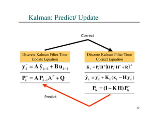
Kalman: Predict/ Update
Discrete Kalman Filter Time
Update Equation
1
1
ˆ −
−
−
+
= k
k
k u
B
y
A
y
Q
P
A
P +
Α
= −
− T
k
k 1
Discrete Kalman Filter Time
Correct Equation
( ) 1
−
−
−
+
= R
H
P
H
H
P
K T
k
T
k
k
)
(
ˆ −
−
−
+
= k
k
k
k
k y
H
x
K
y
y
−
−
= k
k P
H)
K
(I
P
Predict
Correct

13. 13
Notes on Kalman filtering
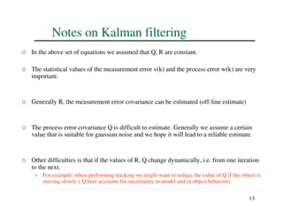
In the above set of equations we assumed that Q, R are constant.
The statistical values of the measurement error v(k) and the process error w(k) are very
important.
Generally R, the measurement error covariance can be estimated (off-line estimate)
The process error covariance Q is difficult to estimate. Generally we assume a certain
value that is suitable for gaussian noise and we hope it will lead to a reliable estimate.
Other difficulties is that if the values of R, Q change dynamically, i.e. from one iteration
to the next.
For example: when performing tracking we might want to reduce the value of Q if the object is
moving slowly ( Q here accounts for uncertainty in model and in object behavior)

14. 14
Applying Kalman filter
Kalman filter is associated with Tracking.
Mainly, all Bayesian estimation family does it.
It has many application when you consider prediction/correction:
Navigation, Sensing , postionning:
Missile tracking.
GPS positioning.
Locating users in GSM networks.
Speech enhancement.
Wireless Communication:
Channel Estimation and Tracking
Computer vision, real

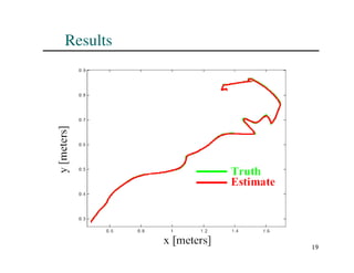
15. 15
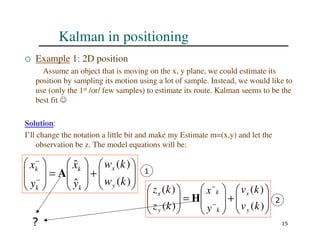
Kalman in positioning
Example 1: 2D position
Assume an object that is moving on the x, y plane, we could estimate its
position by sampling its motion using a lot of sample. Instead, we would like to
use (only the 1st /or/ few samples) to estimate its route. Kalman seems to be the
best fit ☺
Solution:
I’ll change the notation a little bit and make my Estimate m=(x,y) and let the
observation be z. The model equations will be:








+








=








−
−
)
(
)
(
ˆ
ˆ
k
w
k
w
y
x
y
x
y
x
k
k
k
k
A 1








+








=








−
−
)
(
)
(
)
(
)
(
k
v
k
v
y
x
k
z
k
z
y
x
k
k
y
x
H 2
?

16. 16
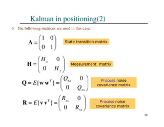
Kalman in positioning(2)
The following matrices are used in this case:








=
1
0
0
1
A State transition matrix








=
=
xx
xx
T
Q
Q
E
0
0
}
{ w
w
Q Process noise
covariance matrix








=
=
xx
xx
T
R
R
E
0
0
}
{ v
v
R Process noise
covariance matrix








=
y
x
H
H
0
0
H Measurement matrix

17. 17
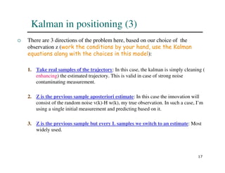
There are 3 directions of the problem here, based on our choice of the
observation z (work the conditions by your hand, use the Kalman
equations along with the choices in this model):
1. Take real samples of the trajectory: In this case, the kalman is simply cleaning (
enhancing) the estimated trajectory. This is valid in case of strong noise
contaminating measurement.
2. Z is the previous sample aposteriori estimate: In this case the innovation will
consist of the random noise v(k)-H w(k), my true observation. In such a case, I’m
using a single initial measurement and predicting based on it.
3. Z is the previous sample but every L samples we switch to an estimate: Most
widely used.
Kalman in positioning (3)

18. 18
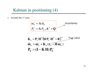
Assume the 1st case:
Kalman in positioning (4)
Q
A
A
A
+
=
=
−
−
−
T
k
k
k
k
P
P
m
m
1
ˆ
( ) 1
−
−
−
+
= R
H
P
H
H
P
K T
k
T
k
k
)
(
ˆ −
−
−
+
= k
k
k
k
k m
H
z
K
m
m
−
−
= k
k P
H)
K
(I
P
Uncertainty
True value

19. 19
Results

20. 20
Significant latency when moving

21. 21
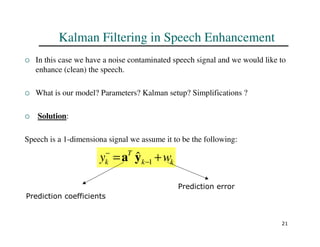
Kalman Filtering in Speech Enhancement
In this case we have a noise contaminated speech signal and we would like to
enhance (clean) the speech.
What is our model? Parameters? Kalman setup? Simplifications ?
Solution:
Speech is a 1-dimensiona signal we assume it to be the following:
k
k
T
k w
y +
= −
−
1
ŷ
a
Prediction coefficients
Prediction error

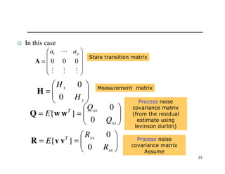
22. 22
In this case










=
M
M
M
L
0
0
0
1 p
a
a
A
State transition matrix








=
=
xx
xx
T
Q
Q
E
0
0
}
{ w
w
Q
Process noise
covariance matrix
(from the residual
estimate using
levinson durbin)








=
=
xx
xx
T
R
R
E
0
0
}
{ v
v
R Process noise
covariance matrix
Assume








=
y
x
H
H
0
0
H Measurement matrix

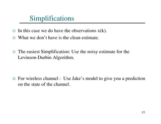
23. 23
Simplifications
In this case we do have the observations x(k).
What we don’t have is the clean estimate.
The easiest Simplification: Use the noisy estimate for the
Levinson-Durbin Algorithm.
For wireless channel : Use Jake’s model to give you a prediction
on the state of the channel.

24. 24
Lecture Activity
Read and Understand the concepts.
Download and understand the simulation of the Kalman filter.
Do the simulation of the Kalmna filter for wireless channel
estimation and tracking.
Read the reading material.
Solve the assignment.

25. 25
References
Brown, R. G. and P. Y. C. Hwang. 1992. Introduction to Random Signals and
Applied Kalman Filtering, Second Edition, John Wiley Sons, Inc.
Gelb, A. 1974. Applied Optimal Estimation, MIT Press, Cambridge, MA.
Grewal, Mohinder S., and Angus P. Andrews (1993). Kalman Filtering Theory
and Practice. Upper Saddle River, NJ USA, Prentice Hall.
Jacobs, O. L. R. 1993. Introduction to Control Theory, 2nd Edition. Oxford
University Press.
Kalman60 Kalman, R. E. 1960. “A New Approach to Linear Filtering and
Prediction Problems,” Transaction of the ASME—Journal of Basic Engineering,
pp. 35-45 (March 1960).
Sorenson70 Sorenson, H. W. 1970. “Least-Squares estimation: from Gauss to
Kalman,” IEEE Spectrum, vol. 7, pp. 63-68, July 1970.