Parallel Bayesian Optimization

Introduction to Parallel Bayesian Optimization
for Machine Learning
Kejia Shi
H2O.ai Inc.
Columbia University in the City of New York
kejia.shi@columbia.edu
August 16, 2017
Kejia Shi Parallel Bayesian Optimization August 16, 2017 1 / 49

Overview
1 Introduction
2 Fundamentals
3 Bayesian Optimization
Gaussian Process
Acquisition Function
4 Parallel Bayesian Optimization

Introduction
So you did all the data cleaning, feature engineering...
And you ﬁt your ﬁrst model with hyperparameters...
Ridge regression: λ...
Neural network: number of layers, batch size...
Random forest: number of trees, leaf size...
Now what you are going to do?

Introduction
θ∗ = arg minθ Φ(θ), for θ ∈ Θ
What is the best set of hyperparameters to optimize the chosen
model?

Problem of Hyperparameter Search
Figure: Typical List of a Convolutional Neural Network Training Hyperparameters

Problem of Hyperparameter Search

Automated Hyperparameter Search: Grid Search

Automated Hyperparameter Search: Random Search

Fundamentals

Fundamentals: Review of Probability
Suppose we have two events, A and B that may or may not be correlated,
A = It’s raining
B = The ground is wet
We can talk about probabilities of these events,
P(A) = Probability it is raining
P(B) = Probability the ground is wet
We can also talk about their other probabilities,
Conditional probabilities
P(B|A) = Probability the ground is wet given that it is raining
Joint probabilities
P(A, B) = Probability it is raining and the ground is wet

Fundamentals: Calculus of Probability
There are simple rules from moving from one probability to another
P(A, B) = P(A|B)P(B) = P(B|A)P(A)
P(A) = ΣbP(A, B = b)
and similarly P(B) = ΣaP(A = a, B)

Fundamentals: Bayes Rule
We want to say something about the probability of B given that A
happened, Bayes rule says that the probability of B after knowing A
is:
P(B|A) =
P(A|B)P(B)
P(A)
.
Notice: P(B|A) – ”posterior”, P(A|B) – ”likelihood”, P(B) – ”prior”
and P(A) – ”marginal” or ”evidence”.

Fundamentals: Gaussian Distribution
x ∼ N(µ, σ2
)
Density: f (x|µ, σ2
) =
1
√
2πσ2
exp{−
(x − µ)2
2σ2
}
Log Density: ln f (x|µ, σ2
) = −
(x − µ)2
2σ2
+ constant

Fundamentals: Probabilistic Model
In short, probabilistic model is a set of probability distribution p(x|).
the distribution family p(·) is selected but we don’t know the
parameter θ.
In Gaussian distribution, p(x|θ), θ = {µ, Σ}.

Fundamentals: Maximum Likelihood
The independent and identically distributed (iid) assumption:
xi
iid
∼ p(x|θ), i = 1, ..., n.
With this, the joint density function becomes
p(x1, ..., xn|θ) = i p(xi |θ).
Maximum likelihood approach seeks the value of θ that mximize the
likelihood function: ˆθML arg maxθ p(x1, ..., xn|θ).
How to solve it? Take gradients!

Fundamentals: Logarithm Trick
Taking gradients of n
i=1 fi p(xi |θ) can be complicated. Therefore we
use the property of monotonically increasing functions on R+.
Speciﬁcally, maximizing g(y) and its monotone transformation
f (g(y)) is the same.
Hence we have the equality
ln(
i
fi ) = Σi ln(fi ).
Notice: location of a maximum does not change, while value of a
maximum does change.
max
y
ln g(y) = max
y
g(y)
arg max
y
ln g(y) = arg max
y
g(y)

Bayesian Optimization

Gaussian Process

Gaussian Process: From Linear Regression
The linear regression model may be written as:
yi ≈ f (xi ; β) = β0 + β1xi1 + β2xi2 + ... + βd xid = β0 + Σd
j=1βj xij .
We have our training data (x1, y1), ..., (xn, yn) and we want to use them to
learn a set of weights β0, β1, ..., βd such that yi ≈ f (xi ; β).
Our least square objective function asks us to choose the β’s that
minimize the sum of squared errors
βLS = argminβΣn
i=1(yi − f (xi ; β))2
≡ argminβL.

Vertical length error. And now (β0, β1, β2) deﬁnes this plane. (Share
the same solution as maximum likelihood approach.)
Idea: Imagine only one feature one response, now you are ﬁtting to a
straight line, which leads to the assumption that errors are normally
distributed.
Extension:
Regularization: l2, Ridge, l1, LASSO
Priors: MAP

Probabistic View
Maximum Likelihood
Likelihood term rising from squared errors y ∼ N(Xβ, σ2I)
βML = argmaxβ ln p(y|µ = Xβ, σ2
)
= argmaxβ −
1
2σ2
||y − Xβ||2
(1)
Maximum a Posteriori
With extra Gaussian prior β ∼ N(0, λ−1I)
Notice ln p(y|X) is unknown. From Bayes Rule:
βMAP = argmaxβ ln p(y|β, X) + ln p(β) − ln p(y|X)
= argmaxβ −
1
2σ2
||y − Xβ||2
−
λ
2
||β||2
(2)

Gaussian Process: In a Bayesian Way
Moving from point estimates to total Bayesian inference:
How do we take into account the uncertainty associated with the
limited data instead of just ﬁnding the MAP solution?
Take oﬀ prior from the likelihood! Instead, build a Gaussian prior
(over weights), Gaussian likelihood model.
(easy for computation of the weights)
The idea is to integrate over multiple straight lines.

Gaussian Process: Bayesian Linear Regression
Settings:
Prior : β ∼ N(0, λ−1
I)
Likelihood : y ∼ N(Xβ, σ2
I)
(3)
The weights don’t even have to be represented explicitly. Different
weights result in different possible possible functions related to your
predictions.
Bayesian linear regression takes into account the imperfect
information and makes subjective guesses with insufficient data.

Inner Product
The inner product of two vectors a = [a1, a2, ..., an] and
b = [b1, b2, ..., bn] is deﬁned as
a · b = Σn
i=1ai bi = a1b1 + a2b2 + ... + anbn.
Inner product operation can be viewed as the simplest kernel function.
K(xn, xm) = xT
n xm.

Gaussian Process: Kernelization
Kernel tricks add more flexibility without changing the algorithm by
efficiently letting you use ”inner product” to frame all kinds of
computation.
Specifically, suppose we have some inputs that cannot be easily
represented as elements of Rd elements, we can still apply a
kernelized algorithm to these inputs, as long as we can define an inner
product on them.
This enable us to integrate over more complicated bases, not just
straight lines to some finite basis (e.g. a polynomial basis {1, x, x2}).

Gaussian Process: Kernelization
Common Kernels
Polynomial kernel: K(xn, xm) = (axT
n xm + c)d , a > 0, c 0, d ∈ Z+
Exponential of a quadratic kernel:
K(xn, xm) = θ0 exp −θ1
2 (xn − xm)T (xn − xm) + θ2 + θ3xT
n xm
Squared exponential kernel:
K(xn, xm) = τ2 exp − 1
2l2 (xn − xm)T (xn − xm)
Mat´ern 3/2 kernel: K(xn, xm) = σ2
f 1 +
√
3r
σl
exp −
√
3r
σl
where,
r = (xn − xm)T (xn − xm).
Mat´ern 5/2 kernel: K(xn, xm) = σ2
f 1 +
√
5r
σl
+ 5r2
3σ2
l
exp −
√
5r
σl

Gaussian Process: Model and Inference
Gaussian Process Model:
Prior: f|X ∼ N(m, K)
Likelihood: y|f , σ2 ∼ N(f, σ2I)
where the elements of the mean vector and kernel/covariance matrix
are deﬁned as mi µ0(xi ) and Ki,j k(xi , xj ).
Posterior:
Mean: µn(x) = µ0(x) + k(x)T (K + σ2I)−1(y − m)
Variance: σ2
n(x) = k(x, x) − k(x)T (K + σ2I)−1k(x)
k(x) is a vector of covariance terms between x and x1:n
These posteriors are used to select the next query point xn+1 as well.

Gaussian Process: Demo and Evaluation
Linear mean function:
- Represents an initial guess at the regression function, with the linear
model m(x) = Xβ corresponding to a convenient special case,
possibly with a hyperprior chosen for the regression coeﬃcients β in
this mean function. Posterior concentrates close to the linear model
to an extent supported by data
Covariance function:
- Controls the smoothness of realizations from the Gaussian process
and the degree of shrinkage towards the mean
Simplicity and ﬂexibility in terms of conditioning and inference!

Gaussian Process: Demo and Evaluation
Advantages
Can ﬁt a wide range of smooth surfaces while being computationally
tractable even for moderate to large numbers of predictors
Disadvantages
O(n3) complexity in terms of total number of observations from the
inversion of a dense covariance matrix
This becomes troublesome as the size of the search space grows with
the model complexity
Solution
Computation becomes signiﬁcantly more accessible and it’s possible
to train many models in parallel

Gaussian Process v.s. Multivariate Gaussian
In short, Gaussian processes can be considered as an inﬁnite-dimensional
generalization of multivariate Gaussian distributions.

Acquisition Function

Acquisition Function: Overview
What does acquisition function mean?
An inexpensive function a(x) that can be evaluated at a given point
x that shows how desirable evaluating f at x is expected to be for
the minimization problem.
How do we query points to evaluate and update our hyperparameters?
Still select arbitrarily?
Utilize our model!

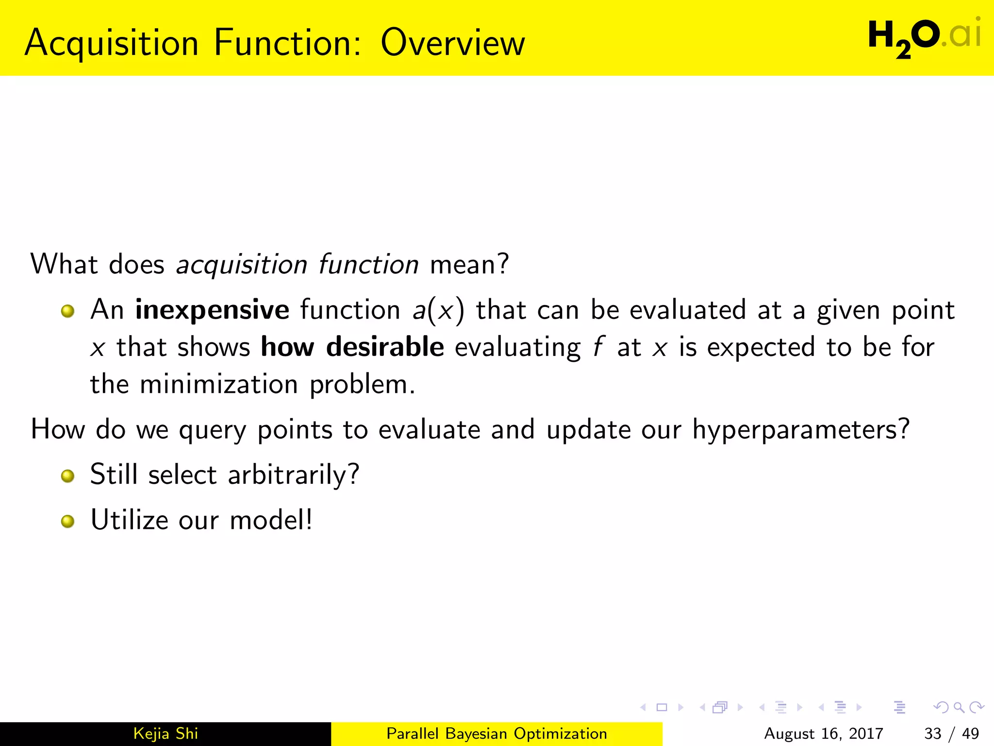
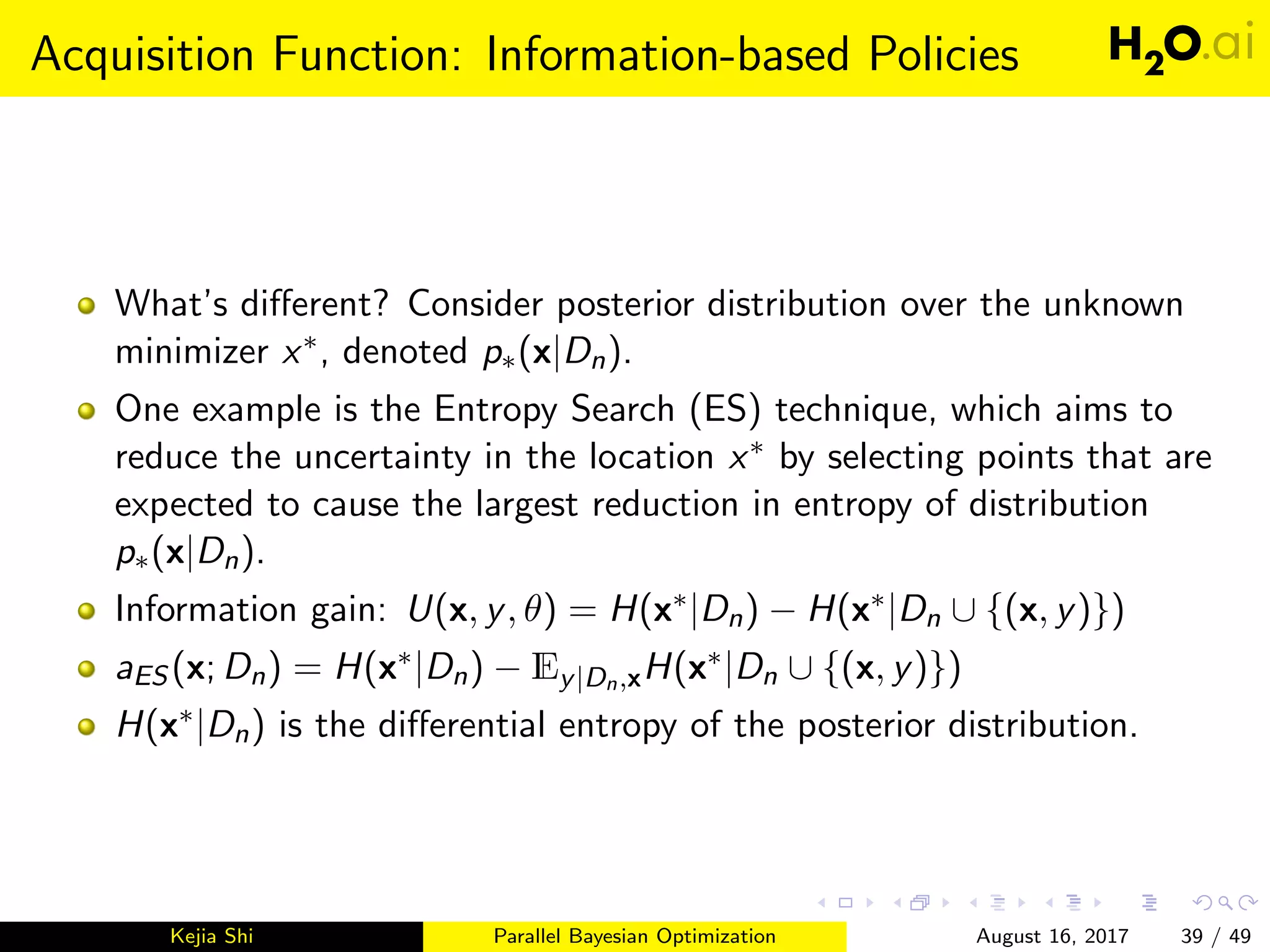
Acquisition Function: Overview
How to utilize the posterior model to create such acquisition functions?
A setting of the model hyperparameters θ
An arbitrary query point x and its correponding function value
v = f (x)
Map them to a utility function U = U(x, v, θ)
Now the acquisition function can be deﬁned as an integration over all its
parameters, i.e. v|x, θ and θ, the selection of the n + 1 point given its
previous data Dn,
a(x; Dn) = EθEv|x,θ[U(x, v, θ)].

Acquisition Function: Marginalization
Deal with a(x; Dn) = EθEv|x,θ[U(x, v, θ)] is very complicated.
We start from the outer expectation over unknown hyperparameters θ.
We wish to marginalize out our uncertainty about θ with
an(x) Eθ|Dn
[a(x; θ)] = a(x; θ)p(θ|Dn)dθ.
Notice: from Bayes Rule, p(θ|Dn) = p(y|X,θ)p(θ)
p(Dn) .
Two ways to tackle the marginalized acquisition function:
Point estimate ˆθ = ˆθML or ˆθMAP , therefore ˆan(x) = a(x; ˆθn).
Sampling from posterior distribution p(θ|Dn), {θ
(i)
n }S
i=1, therefore
Eθ|Dn
[a(x; θ)] ≈ 1
S ΣS
i=1a(x; θ
(i)
n )
Idea: By far we can ignore the θ dependence!

Acquisition Function: Categories
Improvement-based Policies: how much has been improved from
current optimal?
Optimistic Policies: based on our optimistic estimation, what would
this give us? (exploitation and exploration)
Information-based Policies: how much by evaluating this point can
help us reduce the entropy?

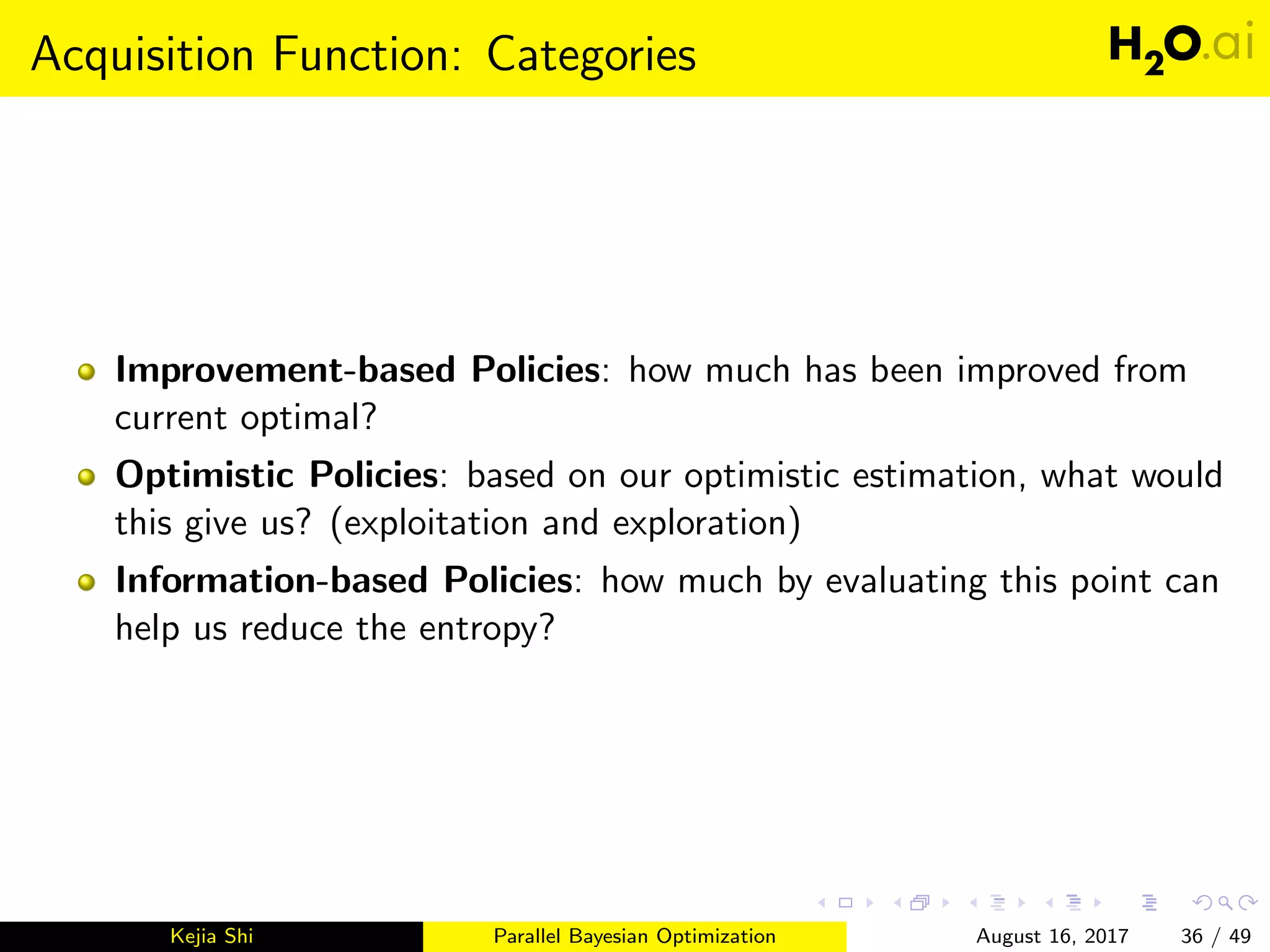
Acquisition Function: Improvement-based Policies
Favors points that are likely to improve upon an incumbent target τ!
Notice τ in practice is set to the best observed value, i.e. maxi=1:n yi .
Probability of improvement(PI):
Earliest idea
aPI (x; Dn) P(v > τ) = Φ(µn(x)−τ
σn(x) )
Expected improvement(EI):
Improvement function, I(x): I(x, v, θ) (v − τ)I(v > τ)
aEI (x; Dn) E[I(x, v, θ)] = (µn(x) − τ)Φ(µn(x)−τ
σn(x) ) + σn(x)φ(µn(x)−τ
σn(x) )

Acquisition Function: Optimistic Policies
As we mentioned acquisition function balances between exploration of
the search space and exploitation of current promising areas, the
upper conﬁdence bound method is one popular way. This category
is optimistic facing uncertainty, as the original method uses the upper
conﬁdence bound as its acquisition function. Since the posterior at
any arbitrary point is a Gaussian, any quantile of the distribution is
computed with its corresponding value of βn as follows,
aUCB(x; Dn) µn(x) + βnσn(x).
We have extra strategies of choosing hyperparameter βn.

Acquisition Function: Information-based Policies
What’s diﬀerent? Consider posterior distribution over the unknown
minimizer x∗, denoted p∗(x|Dn).
One example is the Entropy Search (ES) technique, which aims to
reduce the uncertainty in the location x∗ by selecting points that are
expected to cause the largest reduction in entropy of distribution
p∗(x|Dn).
Information gain: U(x, y, θ) = H(x∗|Dn) − H(x∗|Dn ∪ {(x, y)})
aES (x; Dn) = H(x∗|Dn) − Ey|Dn,xH(x∗|Dn ∪ {(x, y)})
H(x∗|Dn) is the diﬀerential entropy of the posterior distribution.

Acquisition Function: Demo

Parallelization

Parallelization
And more Bayesian optimization packages (scikit-optimize, GPyOpt...)

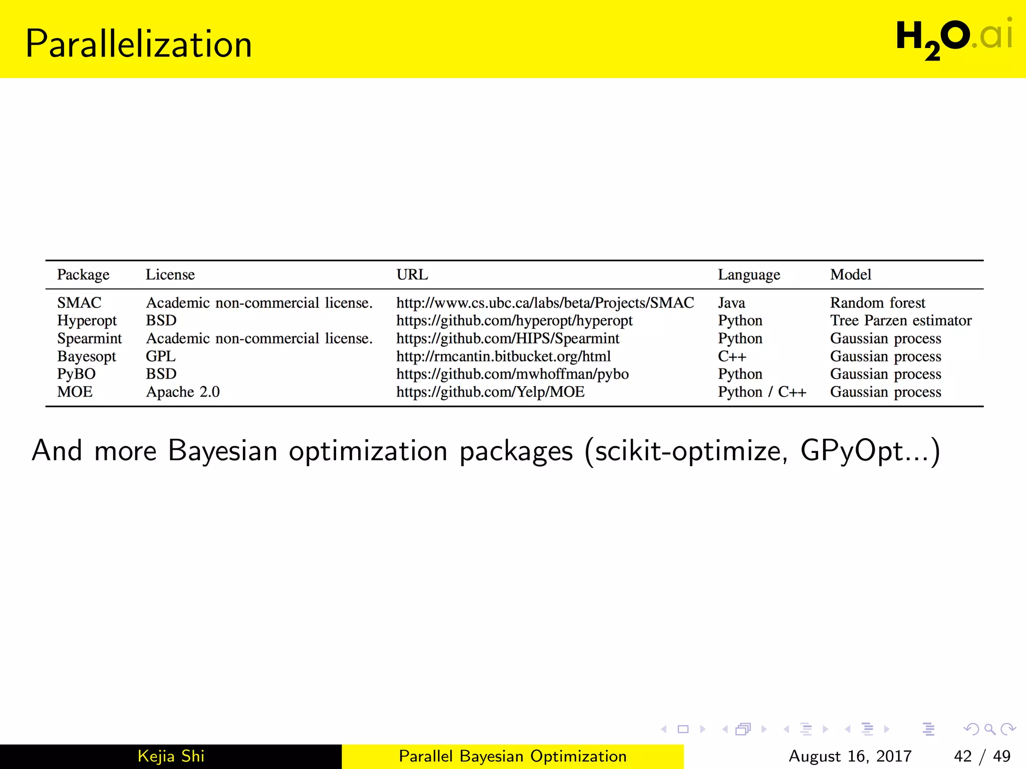
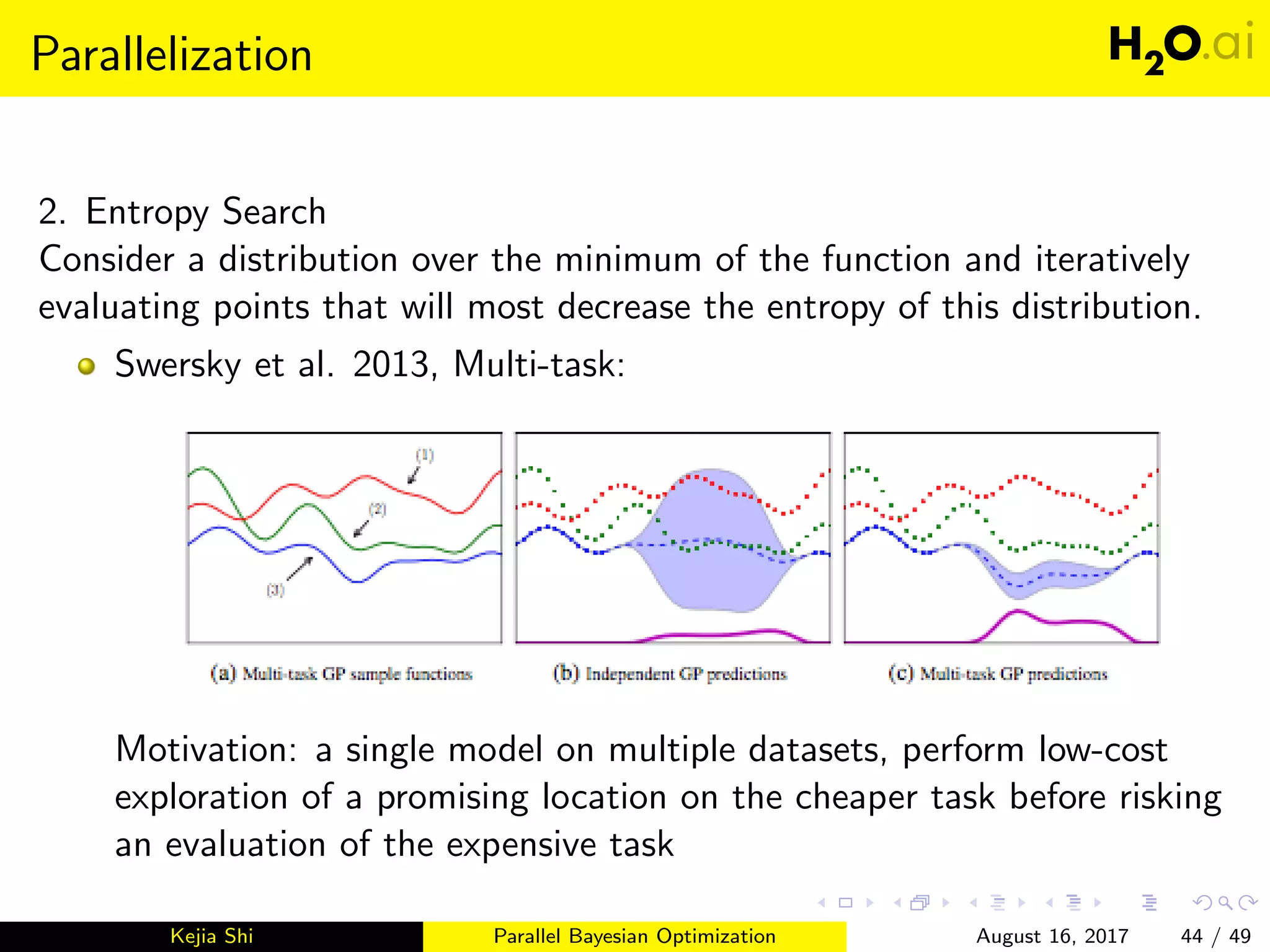
Parallelization
1. On Query Methods (Or Mostly,) Acquisition Function:
Most common: Expected Improvements
Snoek et al. 2012, Spearmint: Monte Carlo Acquisition Function
Wang et al. 2016, MOE (Yelp)[12]: q-EI, argmaxx1, , xqEI(x1, ..., xq)
- Construct an unbiased estimator of EI(x1, , xq) using inﬁnitesimal
perturbation analysis (IPA)
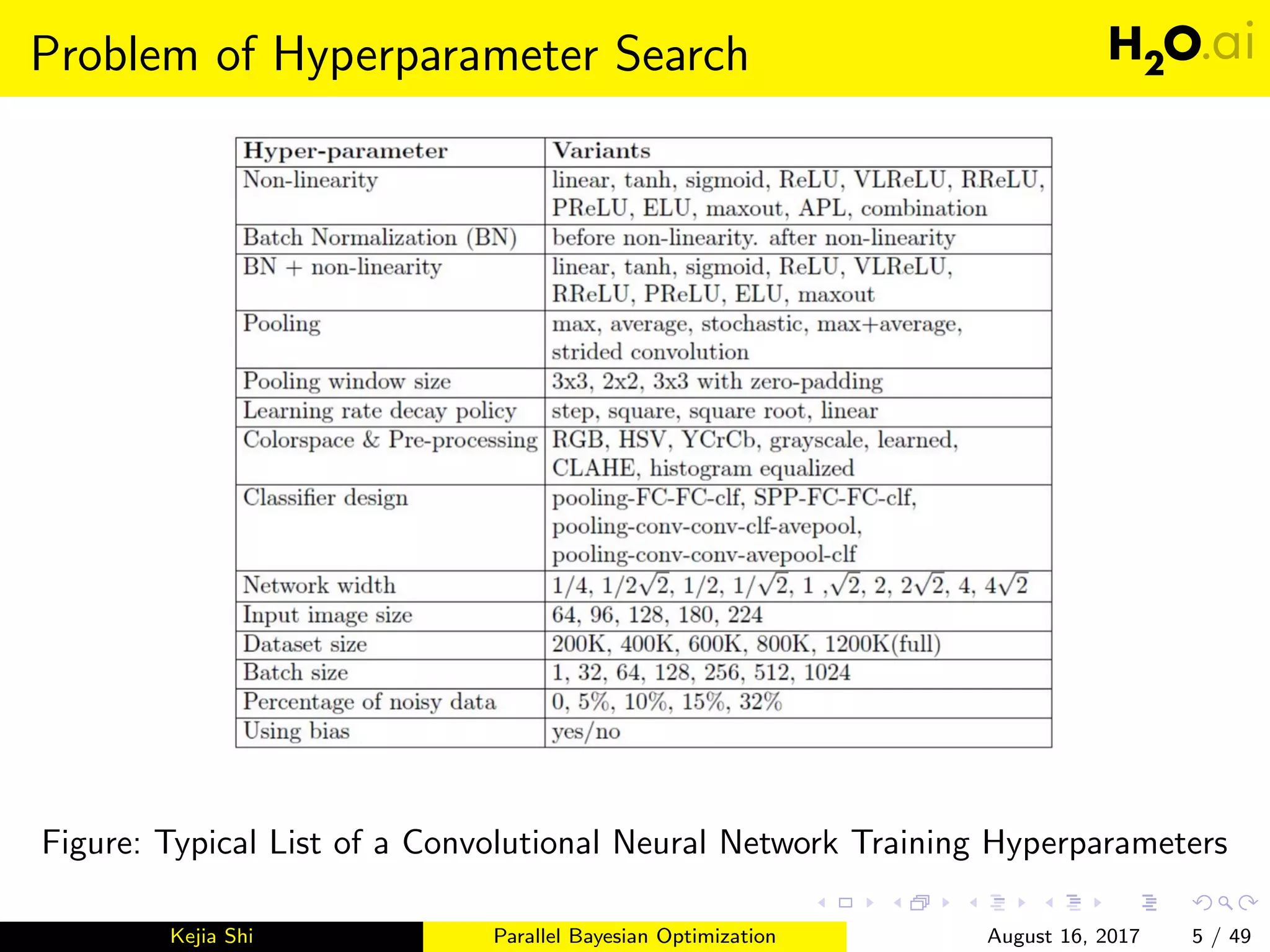
- Turn to a gradient estimator problem under certain assumptions

Parallelization
2. Entropy Search
Consider a distribution over the minimum of the function and iteratively
evaluating points that will most decrease the entropy of this distribution.
Swersky et al. 2013, Multi-task:
Motivation: a single model on multiple datasets, perform low-cost
exploration of a promising location on the cheaper task before risking
an evaluation of the expensive task

Parallelization: Demo
Constant Liar: a constant target value is chosen for all pending new
evaluations (Chevalier, Ginsbourger 2012)

References
0. Fundamentals borrow a lot from Prof. John Paisley’s Machine Learning slides.
Retrieved from http://www.columbia.edu/∼jwp2128/Teaching/W4721/
Spring2017/W4721Spring2017.html
1. Adams, R. P. (2014) A Tutorial on Bayesian Optimization for Machine Learning.
Retrieved from
https://www.iro.umontreal.ca/∼bengioy/.../Ryan adams 140814 bayesopt ncap.pdf
2. Bergstra, J., & Bengio, Y. (2012). Random search for hyper-parameter optimization.
Journal of Machine Learning Research, 13(Feb), 281-305.
3. Gelman, A., Carlin, J. B., Stern, H. S., Dunson, D. B., Vehtari, A., & Rubin, D. B.
(2014). Bayesian Data Analysis (Vol. 2). Boca Raton, FL: CRC press.
4. Hennig, P., & Schuler, C. J. (2012). Entropy Search for Information-Eﬃcient Global
Optimization. Journal of Machine Learning Research, 13(Jun), 18091837.
5. Shahriari, B., Swersky, K., Wang, Z., Adams, R. P., & De Freitas, N. (2016). Taking
the Human Out of the Loop: A Review of Bayesian Optimization. Proceedings of the
IEEE, 104(1), 148175. http://doi.org/10.1109/JPROC.2015.2494218

References
6. Li, L., Jamieson, K., DeSalvo, G., Rostamizadeh, A., & Talwalkar, A. (2016).
Hyperband: A novel bandit-based approach to hyperparameter optimization. arXiv
preprint arXiv:1603.06560.
7. scikit-optimize Package Documentation. Retrieved from
https://scikit-optimize.github.io
8. Snoek, J., Larochelle, H., & Adams, R. P. (2012). Practical bayesian optimization of
machine learning algorithms. In Advances in neural information processing systems (pp.
2951-2959).
9. Swersky, K., Snoek, J., & Adams, R. P. (2013). Multi-task bayesian optimization. In
Advances in neural information processing systems (pp. 2004-2012).

References
Pictures:
1. How CSI Works/Grid Search: https://s-media-cache-
ak0.pinimg.com/originals/3b/dd/d2/3bddd27d048504c1bdb556b17f9ae86e.jpg
2. Catalhoyuk, The team excavates in the South Area on buildings in multiple levels to
better understand the stratigraphy, Retrieved from
(https://www.ﬂickr.com/photos/catalhoyuk/19080999299):
3. A. Honchar, Neural Networks for Algorithmic Trading - Hyperparameters
optimization, Retrieved from (https://medium.com/alexrachnog/neural-networks-for-
algorithmic-trading-hyperparameters-optimization-cb2b4a29b8ee)
4. Grid Search and Random Search Demo Plots, Retrieved from
(http://blog.kaggle.com/2015/07/16/scikit-learn-video-8-eﬃciently-searching-for-
optimal-tuning-parameters/)

The End

Parallel Bayesian Optimization

Recommended

Recommended

More Related Content

What's hot

What's hot (20)

Similar to Parallel Bayesian Optimization

Similar to Parallel Bayesian Optimization (20)

More from Sri Ambati

More from Sri Ambati (20)

Recently uploaded

Recently uploaded (20)

Parallel Bayesian Optimization