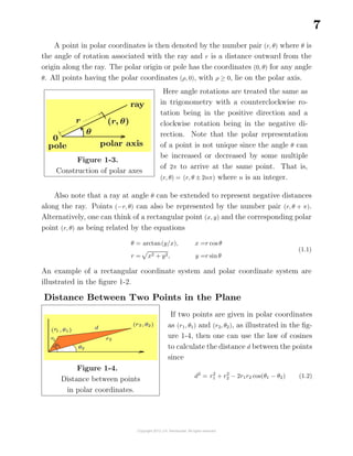
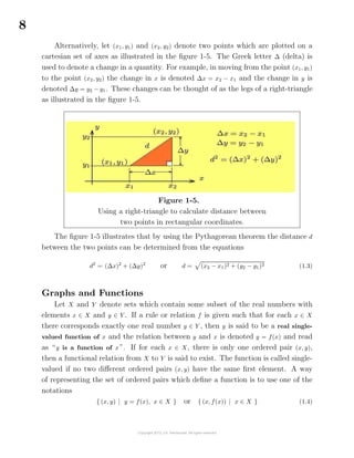
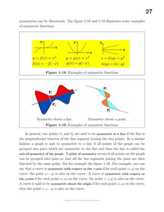
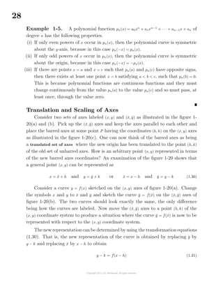
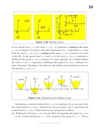
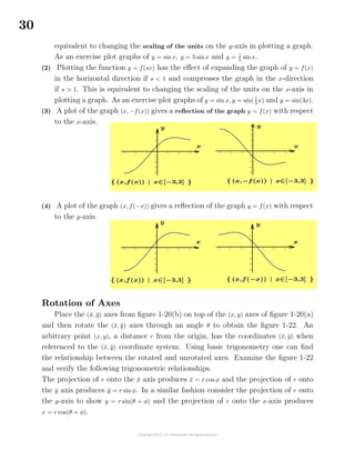
The document provides an introduction to calculus concepts including:
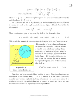
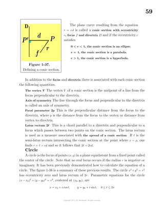
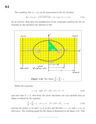
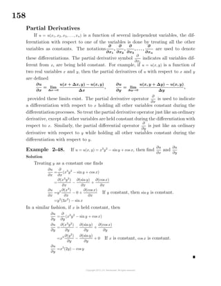
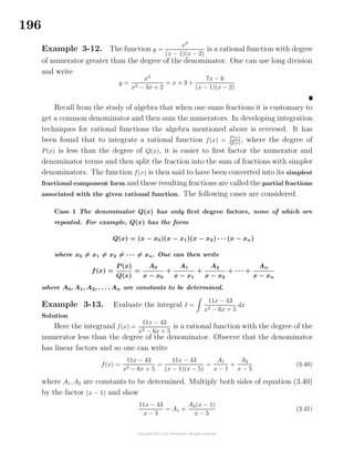
- Sets can represent collections of objects and are denoted using curly brackets. There are five regular solids that follow the Euler formula relating the number of faces, vertices and edges of each solid.
- The preface outlines the main purposes and organization of the two-volume calculus text, which includes fundamental concepts, applications, proofs, and multiple approaches.
- Volume I contains 5 chapters covering sets, functions, graphs, limits, differential calculus, integral calculus, sequences, summations, and applications of calculus.

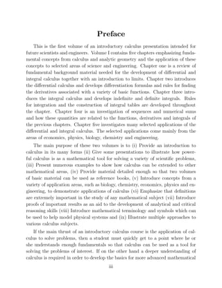
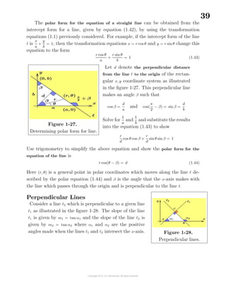
![3
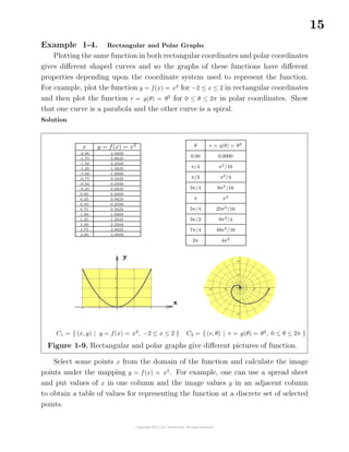
Example 1-1. Intervals
When dealing with real numbers a, b, x it is customary to use the following no-
tations to represent various intervals of real numbers.
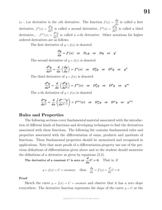
Set Notation Set Definition Name
[a, b] {x | a ≤ x ≤ b} closed interval
(a, b) {x | a < x < b} open interval
[a, b) {x | a ≤ x < b} left-closed, right-open
(a, b] {x | a < x ≤ b} left-open, right-closed
(a, ∞) {x | x > a} left-open, unbounded
[a, ∞) {x | x ≥ a} left-closed,unbounded
(−∞, a) {x | x < a} unbounded, right-open
(−∞, a] {x | x ≤ a} unbounded, right-closed
(−∞, ∞) R = {x | −∞ < x < ∞} Set of real numbers
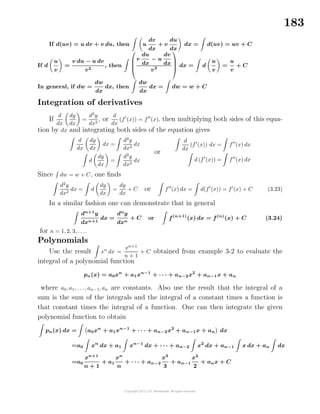
Subsets
If for every element x ∈ A one can show that x is also an element of a set B,
then the set A is called a subset of B or one can say the set A is contained in the
set B. This is expressed using the mathematical statement A ⊂ B, which is read “A
is a subset of B ”. This can also be expressed by saying that B contains A, which is
written as B ⊃ A. If one can find one element of A which is not in the set B, then A
is not a subset of B. This is expressed using either of the notations A ⊂ B or B ⊃ A.
Note that the above definition implies that every set is a subset of itself, since the
elements of a set A belong to the set A. Whenever A ⊂ B and A = B, then A is called
a proper subset of B.
Set Operations
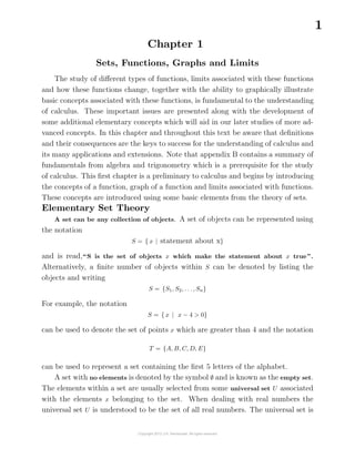
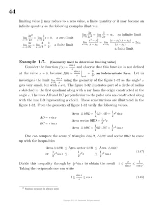
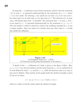
Given two sets A and B, the union of these sets is written A ∪ B and defined
A ∪ B = { x | x ∈ A or x ∈ B, or x ∈ both A and B}
The intersection of two sets A and B is written A ∩ B and defined
A ∩ B = { x | x ∈ both A and B }
If A ∩ B is the empty set one writes A ∩ B = ∅ and then the sets A and B are said to
be disjoint.](https://image.slidesharecdn.com/calculusvolume-1-160216221448/85/Calculus-volume-1-11-320.jpg)
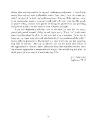
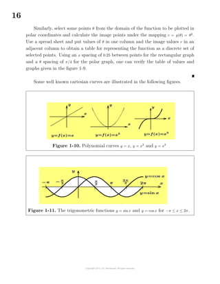
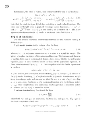
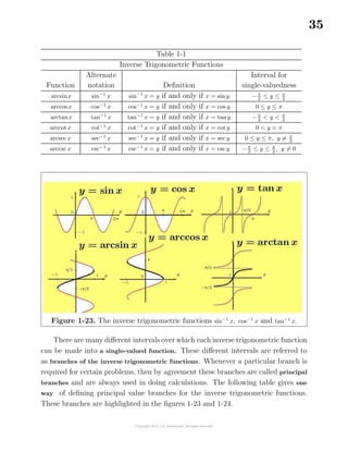
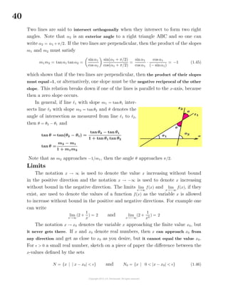
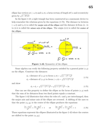
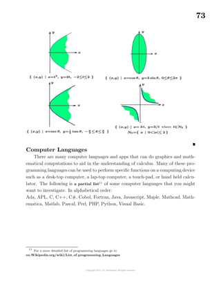
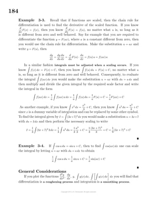
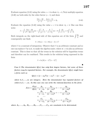
![10
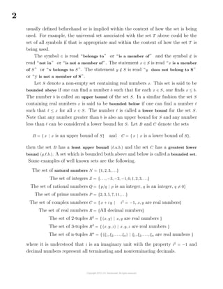
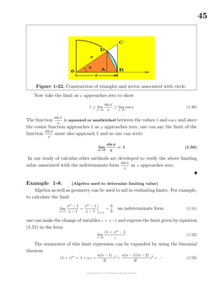
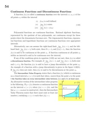
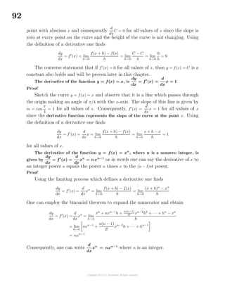
called the locus of points satisfying the rule. The graph illustrated in the figure 1-6
is a pictorial representation of the given rule.
x y = f(x) = x2 + x
-2.0 2.00
-1.8 1.44
-1.6 0.96
-1.4 0.56
-1.2 0.24
-1.0 0.00
-0.8 -0.16
-0.6 -0.24
-0.4 -0.24
-0.2 -0.16
0.0 0.00
0.2 0.24
0.4 0.56
0.6 0.96
0.8 1.44
1.0 2.00
1.2 2.64
1.4 3.36
1.6 4.16
1.8 5.04
2.0 6.00
Figure 1-6. A graph of the function y = f(x) = x2
+ x
Note that substituting x + h in place of x in the function rule gives
f(x + h) = (x + h)2
+ (x + h) = x2
+ (2h + 1)x + (h2
+ h).
If f(x) represents the height of the curve at the point x, then f(x + h) represents the
height of the curve at x + h.
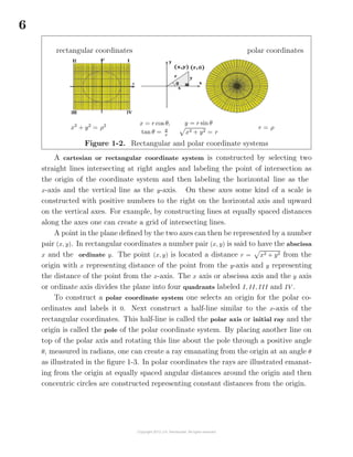
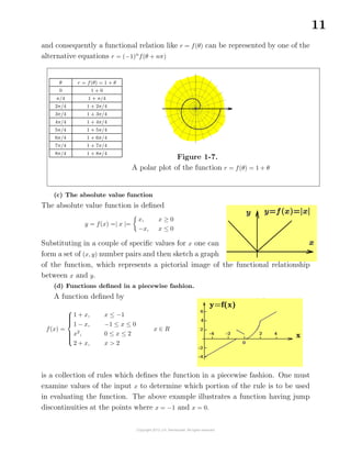
(b) Let r = f(θ) = 1 + θ for 0 ≤ θ ≤ 2π be a given rule defining a function which
can be represented by a curve in polar coordinates (r, θ). One can select a set
of ordered values for θ in the interval [0, 2π] and calculate the corresponding
values for r = f(θ). The set of points (r, θ) created can then be plotted on polar
graph paper to give a pictorial representation of the function rule. The graph
illustrated in the figure 1-7 is a pictorial representation of the given function
over the given domain.
Note in dealing with polar coordinates a radial distance r and polar angle θ can
have any of the representations
((−1)n
r, θ + nπ)](https://image.slidesharecdn.com/calculusvolume-1-160216221448/85/Calculus-volume-1-18-320.jpg)
![42
In terms of limits, if α and β are infinitesimals and lim
α→0
β
α
is some constant
different from zero, then α and β are called infinitesimals of the same order. However,
if lim
α→0
β
α
= 0, then β is called an infinitesimal of higher order than α.
If you are dealing with an equation involving infinitesimals of different
orders, you only need to retain those infinitesimals of lowest order, since the higher
order infinitesimals are significantly smaller and will not affect the results
when these infinitesimals approach zero .
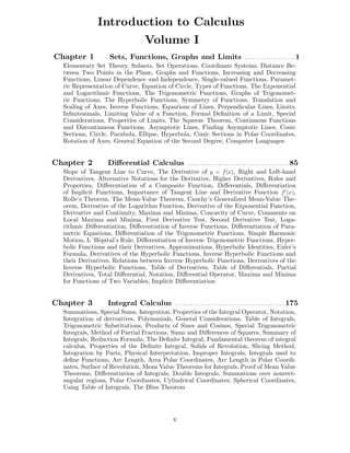
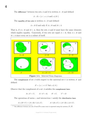
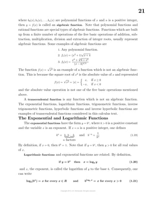
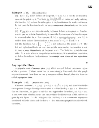
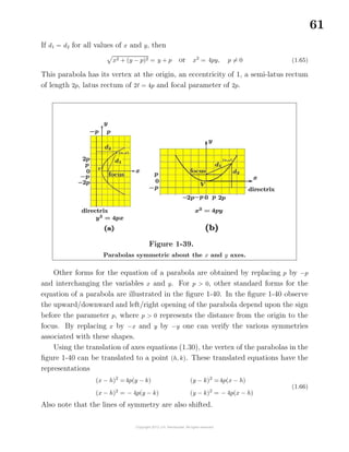
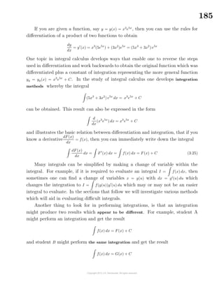
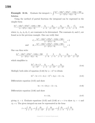
This concept is often used in comparing the ratio of two small quantities which
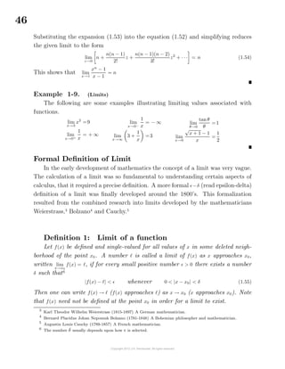
approach zero. Consider the problem of finding the volume of a hollow cylinder, as
illustrated in the figure 1-30, as the thickness of the cylinder sides approaches zero.
Figure 1-30. Volume of hollow cylinder.
Let ∆V denote the volume of the hollow cylinder with r the inner radius of the
hollow cylinder and r + ∆r the outer radius. One can write
∆V =Volume of outer cylinder − Volume of inner cylinder
∆V =π(r + ∆r)2
h − πr2
h = π[r2
+ 2r∆r + (∆r)2
]h − πr2
h
∆V =2πrh∆r + πh(∆r)2
This relation gives the exact volume of the hollow cylinder. If one takes the limit
as ∆r tends toward zero, then the ∆r and (∆r)2
terms become infinitesimals and
the infinitesimal of the second order can be neglected since one is only interested in
comparison of ratios when dealing with small quantities. For example
lim
∆r→0
∆V
∆r
= lim
∆r→0
(2πrh + πh∆r) = 2πrh](https://image.slidesharecdn.com/calculusvolume-1-160216221448/85/Calculus-volume-1-50-320.jpg)
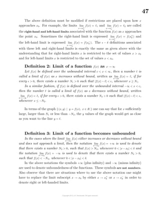
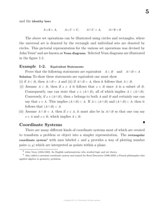
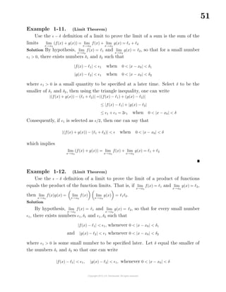
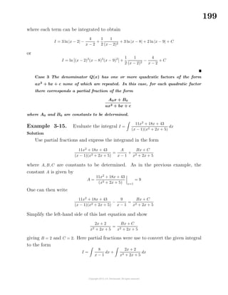
![49
The shaded rectangle consists of the set of values
S = { (x, y) | 0 < |x − x0| < δ and |y − | < }
Note that the line where x = x0 and − < y < + is excluded from the set. The
problem is that for every > 0 that is specified, one must know how to select the
δ to insure the curve stays within the shaded rectangle. If this can be done then
is defined to be the lim
x→x0
f(x). In order to make |f(x) − | small, as x → x0, one must
restrict the values of x to some small deleted neighborhood of the point x0. If only
points near x0 are to be considered, it is customary to always select δ to be less than
or equal to 1. Thus if |x − x0| < 1, then x is restricted to the interval [x0 − 1, x0 + 1].
Example 1-10. ( − δ proof)
Use the − δ definition of a limit to prove that lim
x→3
x2
= 9
Solution
Here f(x) = x2
and = 9 so that
|f(x) − | = |x2
− 9| = |(x + 3)(x − 3)| = |x + 3| · |x − 3| (1.56)
To make |f(x) − | small one must control the size of |x − 3|. Recall that by agreement
δ is to be selected such that δ < 1 and as a consequence of this the statement “x is
near 3” is to mean x is restricted to the interval [2, 4]. This information allows us to
place bounds upon the factor (x + 3). That is, |x + 3| < 7, since x is restricted to the
interval [2, 4]. One can now use this information to change equation (1.56) into an
inequality by noting that if |x − 3| < δ, one can then select δ such that
|f(x) − | = |x2
− 9| = |x + 3| · |x − 3| < 7δ < (1.57)
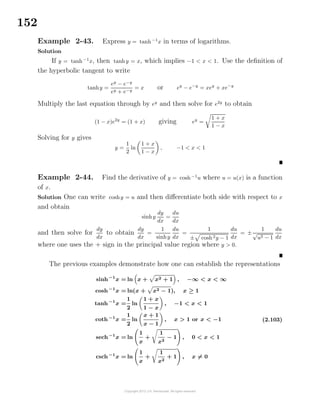
where > 0 and less than 1, is as small as you want it to be. The inequality (1.57)
tells us that if δ < /7, then it follows that
|x2
− 9| < whenever |x − 3| < δ
Special Considerations
1. The quantity used in the definition of a limit is often replaced by some scaled
value of , such as α , 2
,
√
, etc. in order to make the algebra associated with
some theorem or proof easier.](https://image.slidesharecdn.com/calculusvolume-1-160216221448/85/Calculus-volume-1-57-320.jpg)
![50
2. The limiting process has the property that for f(x) = c, a constant, for all values
of x, then
lim
x→x0
c = c (1.58)
This is known as the constant function rule for limits.
3. The limiting process has the property that for f(x) = x, then lim
x→x0
x = x0.
This is sometimes called the identity function rule for limits.
Properties of Limits
If f(x) and g(x) are functions and the limits lim
x→x0
f(x) = 1 and lim
x→x0
g(x) = 2 both
exist and are finite, then
(a) The limit of a constant times a function equals the constant times the limit of
the function.
lim
x→x0
cf(x) = c lim
x→x0
f(x) = c 1 for all constants c
(b) The limit of a sum is the sum of the limits.
lim
x→x0
[f(x) + g(x)] = lim
x→x0
f(x) + lim
x→x0
g(x) = 1 + 2
(c) The limit of a difference is the difference of the limits.
lim
x→x0
[f(x) − g(x)] = lim
x→x0
f(x) − lim
x→x0
g(x) = 1 − 2
(d) The limit of a product of functions equals the product of the function limits.
lim
x→x0
[f(x) · g(x)] = lim
x→x0
f(x) · lim
x→x0
g(x) = 1 · 2
(e) The limit of a quotient is the quotient of the limits provided that the denom-
inator limit is nonzero.
lim
x→x0
f(x)
g(x)
=
lim
x→x0
f(x)
lim
x→x0
g(x)
=
1
2
, provided 2 = 0
(f) The limit of an nth root is the nth root of the limit.
lim
x→x0
n
f(x) = n lim
x→x0
f(x) =
n
√
1
if n is an odd positive integer or
if n is an even positive integer and 1 > 0
(g) Repeated applications of the product rule with g(x) = f(x) gives the extended
product rule.
lim
x→x0
f(x)n
= lim
x→x0
f(x)
n
(h) The limit theorem for composite functions is as follows.
If lim
x→x0
g(x) = , then lim
x→x0
f(g(x)) = f lim
x→x0
g(x) = f( )](https://image.slidesharecdn.com/calculusvolume-1-160216221448/85/Calculus-volume-1-58-320.jpg)
![57
4. The line y = y0 is called a horizontal asymptote if one of the following condi-
tions is true.
lim
x→∞
f(x) = y0, lim
x→−∞
f(x) = y0
5. The line y = mx + b is called a slant asymptote or oblique asymptote if
lim
x→∞
[f(x) − (mx + b)] = 0
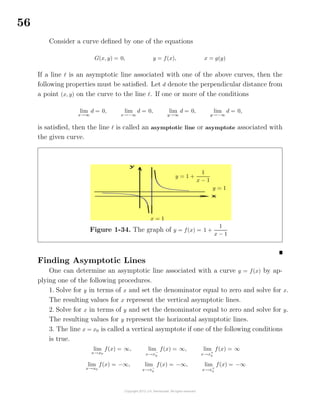
Example 1-16. Asymptotic Lines
Consider the curve y = f(x) = 2x + 1 +
1
x
, where x ∈ R. This function has the
properties that
lim
x→∞
[f(x) − (2x + 1)] = lim
x→∞
1
x
= 0 and lim
x→0
f(x) = ±∞
so that one can say the line y = 2x + 1 is an oblique asymptote and the line x = 0 is
a vertical asymptote. A sketch of this curve is given in the figure 1-35.
Figure 1-35. Sketch of curve y = f(x) = 2x + 1 +
1
x
y = 2x + 1
x = 0
Conic Sections
A general equation of the second degree has the form
Ax2
+ Bxy + Cy2
+ Dx + Ey + F = 0 (1.64)
where A, B, C, D, E, F are constants. All curves which have the form of equation (1.64)
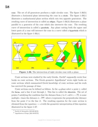
can be obtained by cutting a right circular cone with a plane. The figure 1-36(a)
illustrates a right circular cone obtained by constructing a circle in a horizontal plane
and then moving perpendicular to the plane to a point V above or below the center
of the circle. The point V is called the vertex of the cone. All the lines through the
point V and points on the circumference of the circle are called generators of the](https://image.slidesharecdn.com/calculusvolume-1-160216221448/85/Calculus-volume-1-65-320.jpg)

![76
1-13. Sketch a graph of the given functions.
(a) y =
1
2
x, y = x, y = 2x, −4 ≤ x ≤ 4
(b) y =
1
4
x2
, y = x2
, y = 4x2
, −4 ≤ x ≤ 4
(c) y =
1
2
sin x, y = sinx, y = 2 sinx, 0 ≤ x ≤ 2π
(d) y =
1
2
cos x, y = cos x, y = 2 cos x, 0 ≤ x ≤ 2π
1-14. Sketch the graphs defined by the parametric equations.
(a) Ca = { (x, y) | x = t2
, y = 2t + 1, 0 ≤ t ≤ 4 }
(b) Cb = { (x, y) | x = t, y = 2t + 1, −2 ≤ t ≤ 2 }
(c) Cc = { (x, y) | x = cos t, y = sin t,
π
2
≤ t ≤
3π
2
}
(d) Cd = { (x, y) | x = sint, y = cos t, 0 ≤ t ≤ π }
(e) Ce = { (x, y) | x = t, y = − 9 − t2, −3 ≤ t ≤ 3 }
Note that the part of the curve represented depends on (i) the form of the parametric
representation and (ii) the values assigned to the parameters.
1-15. Sketch a graph of the given polynomial functions for x ∈ R.
(a) y = x − 1 (b) y = x2
− 2x − 3 (c) y = (x − 1)(x − 2)(x − 3)
(d) Show the function y = (x−1)(x−2)(x−3) is skew-symmetric about the line x = 2.
1-16. The Heaviside12
step function is defined
H(ξ) =
0, ξ < 0
1, ξ > 0
Sketch the following functions.
(a) y = H(x)
(b) y = H(x − 1)
(c) y = H(x − 2)
(d) y = H(x − 1) − H(x − 2)
(e) y = H(x) + H(x − 1) − 2H(x − 2)
(f) y =
1
[H(x − x0) − H(x − (x0 + ))], > 0 is small.
12
Oliver Heaviside (1850-1925) An English engineer.](https://image.slidesharecdn.com/calculusvolume-1-160216221448/85/Calculus-volume-1-84-320.jpg)
![80
1-33. Sketch a graph of the following straight lines. State the slope of each line
and specify the x or y-intercept if it exists.
(a) x = 5
(b) y = 5
(c) y = x + 1
(d) 3x + 4y + 5 = 0
(e)
x
3
+
y
4
= 1
(f) = { (x, y) | x = t + 2, y = 2t + 3 }
(g) r cos(θ − π/4) = 2
(h) 3x + 4y = 0
1-34. For each line in the previous problem construct the perpendicular bisector
which passes through the origin.
1-35. Consider the function y = f(x) =
x2
− 1
x − 1
, for −2 ≤ x ≤ 2.
(a) Is f(1) defined?
(b) Is the function continuous over the interval −2 ≤ x ≤ 2?
(c) Find lim
x→1
f(x)
(d) Can f(x) be made into a continuous function?
(e) Sketch the function f(x).
1-36. Assume lim
x→x0
f(x) = 1 and lim
x→x0
g(x) = 2. Use the − δ proof to show that
lim
x→x0
[f(x) − g(x)] = 1 − 2
1-37.
(a) Find the equation of the line with slope 2 which passes through the point (3, 4).
(b) Find the equation of the line perpendicular to the line in part (a) which passes
through the point (3, 4).
1-38. Find the following limits if the limit exists.
(a) lim
x→1
x2
+
1
x
(b) lim
x→0
2x
+
1
2x
(c) lim
h→0
√
x + h −
√
x
h x(x + h)
, x = 0
(d) lim
h→0
f(x + h) − f(x)
h
, f(x) = x2
(e) lim
x→2
x − 2
x2 + x − 6
(f) lim
x→2
x − 2
x2 − 4](https://image.slidesharecdn.com/calculusvolume-1-160216221448/85/Calculus-volume-1-88-320.jpg)
![85
Chapter 2
Differential Calculus
The history of mathematics presents the development of calculus as being ac-
credited to Sir Isaac Newton (1642-1727) an English physicist, mathematician and
Gottfried Wilhelm Leibnitz (1646-1716) a German physicist, mathematician. Por-
traits of these famous individuals are given in the figure 2-1. The introduction of
calculus created an explosion in the development of the physical sciences and other
areas of science as calculus provided a way of describing natural and physical laws
in a mathematical format which is easily understood. The development of calculus
also opened new areas of mathematics and science as individuals sought out new
ways to apply the techniques of calculus.
Figure 2-1. Joint developers of the calculus.
Calculus is the study of things that change and finding ways to represent these
changes in a mathematical way. The symbol ∆ will be used to represent change.
For example, the notation ∆y is to be read “The change in y”.
Slope of Tangent Line to Curve
Consider a continuous smooth1
curve y = f(x), defined over a closed interval
defined by the set of points X = { x | x ∈ [a, b] }. Here x is the independent variable, y
1
A continuous smooth curve is an unbroken curve defined everywhere over the domain of definition of the
function and is a curve which has no sharp edges. If P is a point on the curve and is the tangent line to the point
P, then a smooth curve is said to have a continuously turning tangent line as P moves along the curve.](https://image.slidesharecdn.com/calculusvolume-1-160216221448/85/Calculus-volume-1-93-320.jpg)
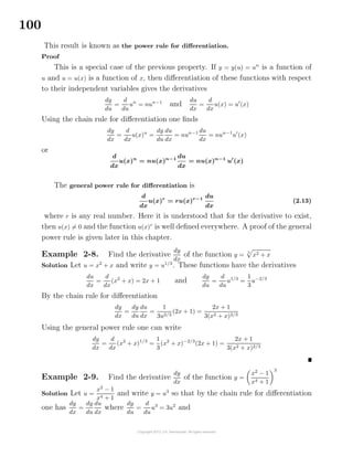
![93
Later it will be demonstrated that
d
dx
xr
= rxr−1
for all real numbers r which
are different from zero.
The derivative of a constant times a function equals the constant times the deriva-
tive of the function or
d
dx
[Cf(x)] = C
d
dx
f(x) = Cf (x)
Proof
Use the definition of a derivative applied to the function g(x) = Cf(x) and show
that
d
dx
g(x) = lim
h→0
g(x + h) − g(x)
h
= lim
h→0
Cf(x + h) − Cf(x)
h
= lim
h→0
C
f(x + h) − f(x)
h
It is known that the limit of a constant times a function is the constant times the
limit of the function and so one can write
d
dx
g(x) = C lim
h→0
f(x + h) − f(x)
h
= Cf (x)
or
d
dx
[Cf(x)] = C
d
dx
f(x) = Cf (x)
The derivative of a sum is the sum of the derivatives or
d
dx
[u(x) + v(x)] =
d
dx
u(x) +
d
dx
v(x) =
du
dx
+
dv
dx
= u (x) + v (x) (2.4)
This result can be extended to include n-functions
d
dx
[u1(x) + u2(x) + · · · + un(x)] =
d
dx
u1(x) +
d
dx
u2(x) + · · · +
d
dx
un(x)
Proof
If y(x) = u(x) + v(x), then
dy
dx
= lim
h→0
y(x + h) − y(x)
h
= lim
h→0
u(x + h) + v(x + h) − [u(x) + v(x)]
h
= lim
h→0
u(x + h) − u(x)
h
+ lim
h→0
v(x + h) − v(x)
h
or
dy
dx
=
d
dx
[u(x) + v(x)] =
d
dx
u(x) +
d
dx
v(x) = u (x) + v (x)
This result follows from the limit property that the limit of a sum is the sum of
the limits. The above proof can be extended to larger sums by breaking the larger
sums into smaller groups of summing two functions.](https://image.slidesharecdn.com/calculusvolume-1-160216221448/85/Calculus-volume-1-101-320.jpg)
![94
Example 2-4. The above properties are combined into the following examples.
(a) If y = F(x) is a function which is differentiable and C is a nonzero constant, then
d
dx
[CF(x)] =C
dF(x)
dx
d
dx
[F(x) + C] =
dF(x)
dx
+
d
dx
C =
dF(x)
dx
d
dx
5x3
=5
d
dx
x3
= 5(3x2
) = 15x2
d
dx
x3
+ 8 =
d
dx
x3
+
d
dx
8 = 3x2
since the derivative of a constant times a function equals the constant times
the derivative of the function and the derivative of a sum is the sum of the
derivatives.
(b) If S = {f1(x), f2(x), f3(x), . . ., fn(x), . . . } is a set of functions, define the set of deriva-
tives
dS
dx
= {
df1
dx
,
df2
dx
,
df3
dx
, . . .,
dfn
dx
, . . . }. To find the derivatives of each of the func-
tions in the set S = {1, x, x2
, x3
, x4
, x5
, . . ., x100
, . . ., xm
, . . . }, where m is a very large
integer, one can use properties 1 , 2 and 3 above to write
dS
dx
= {0, 1, 2x, 3x2
, 4x3
, 5x4
, . . ., 100x99
, . . ., mxm−1
, . . . }
(c) Consider the polynomial function y = x6
+ 7x4
+ 32x2
− 17x + 33. To find the
derivative of this function one can combine the properties 1, 2, 3, 4 to show
dy
dx
=
d
dx
(x6
+ 7x4
+ 32x2
− 17x + 33)
dy
dx
=
d
dx
x6
+ 7
d
dx
x4
+ 32
d
dx
x2
− 17
d
dx
x +
d
dx
(33)
dy
dx
=6x5
+ 7(4x3
) + 32(2x) − 17(1) + 0
dy
dx
=6x5
+ 28x3
+ 64x − 17
This result follows from use of the properties (i) the derivative of a sum is the
sum of the derivatives (ii) the derivative of a constant times a function is that
constant times the derivative of the function (iii) the derivative of x to a power
is the power times x to the one less power and (iv) the derivative of a constant
is zero.
(d) To find the derivative of a polynomial function
y = pn(x) = a0xn
+ a1xn−1
+ a2xn−2
+ · · · + an−2x2
+ an−1x + an, (2.5)
where a0, a1, . . ., an are constants,with a0 = 0, one can use the first four proper-
ties above to show that by differentiating each term one obtains the derivative
function
dy
dx
= a0 nxn−1
+ a1 (n − 1)xn−2
+ a2 (n − 2)xn−3
+ · · ·an−2 [2x] + an−1[1] + 0](https://image.slidesharecdn.com/calculusvolume-1-160216221448/85/Calculus-volume-1-102-320.jpg)
![95
(e) The polynomial function pn(x) of degree n given by equation (2.5) is a linear
combination of terms involving x to a power. The first term a0xn
, with a0 = 0,
being the term containing the largest power of x. Make note of the higher
derivatives associated with the function xn
. These derivatives are
d
dx
(xn
) =nxn−1
d2
dx2
(xn
) =n(n − 1)xn−2
d3
dx3
(xn
) =n(n − 1)(n − 2)xn−3
...
...
dn
dxn
(xn
) =n(n − 1)(n − 2) · · ·(3)(2)(1)x0
= n! Read n-factorial.
dn+1
dxn+1
(xn
) =0
This result demonstrates that the (n+1)st and higher derivatives of a polynomial
of degree n will all be zero.
(f) One can readily verify the following derivatives
d3
dx3
(x3
) =3! = 3 · 2 · 1 = 6
d4
dx4
(x3
) =0
d5
x5
(x5
) =5! = 5 · 4 · 3 · 2 · 1 = 120
d6
dx6
(x5
) =0
The derivative of a product of two functions is the first function times the deriva-
tive of the second function plus the second function times the derivative of the first
function or
d
dx
[u(x)v(x)] =u(x)
dv
dx
+ v(x)
du
dx
= u(x)v (x) + v(x)u (x)
or
d
dx
[u(x)v(x)] =u(x)v(x)
u (x)
u(x)
+
v (x)
v(x)
(2.6)
Proof
Use the properties of limits along with the definition of a derivative to show that if
y(x) = u(x)v(x), then
dy
dx
= lim
h→0
y(x + h) − y(x)
h
= lim
h→0
u(x + h)v(x + h) − u(x)v(x)
h
= lim
h→0
u(x + h)v(x + h) − u(x)v(x + h) + u(x)v(x + h) − u(x)v(x)
h](https://image.slidesharecdn.com/calculusvolume-1-160216221448/85/Calculus-volume-1-103-320.jpg)
![96
Where the term u(x)v(x + h) has been added and subtracted to the numerator.
Now rearrange terms and use the limit properties to write
dy
dx
= lim
h→0
u(x + h) − u(x)
h
v(x + h) + lim
h→0
u(x)
v(x + h) − v(x)
h
dy
dx
= lim
h→0
u(x) lim
h→0
v(x + h) − v(x)
h
+ lim
h→0
v(x + h) lim
h→0
u(x + h) − u(x)
h
or
dy
dx
=
d
dx
[u(x)v(x)] = u(x)
dv
dx
+ v(x)
du
dx
= u(x)v (x) + v(x)u (x)
The result given by equation (2.6) is known as the product rule for differentiation.
Example 2-5.
(a) To find the derivative of the function y = (3x2
+2x+1)(8x+3) one should recognize
the function is defined as a product of polynomial functions and consequently
the derivative is given by
dy
dx
=
d
dx
(3x2
+ 2x + 1)(8x + 3)
dy
dx
=(3x2
+ 2x + 1)
d
dx
(8x + 3) + (8x + 3)
d
dx
(3x2
+ 2x + 1)
dy
dx
=(3x2
+ 2x + 1)(8) + (8x + 3)(6x + 2)
dy
dx
=72x2
+ 50x + 14
(b) The second derivative is by definition a derivative of the first derivative so that
differentiating the result in part(a) gives
d2
y
dx2
=
d
dx
dy
dx
=
d
dx
72x2
+ 50x + 14 = 144x + 50
Similarly, the third derivative is
d3
y
dx3
=
d
dx
d2
y
dx2
=
d
dx
(144x + 50) = 144
and the fourth derivative and higher derivatives are all zero.
Example 2-6.
Consider the problem of differentiating the function y = u(x)v(x)w(x) which is a
product of three functions. To differentiate this function one can apply the product
rule to the function y = [u(x)v(x)] · w(x) to obtain](https://image.slidesharecdn.com/calculusvolume-1-160216221448/85/Calculus-volume-1-104-320.jpg)
![97
dy
dx
=
d
dx
([u(x)v(x)] · w(x)) = [u(x)v(x)]
dw(x)
dx
+ w(x)
d
dx
[u(x)v(x)]
Applying the product rule to the last term one finds
dy
dx
=
d
dx
[u(x)v(x)w(x)] = u(x)v(x)
dw(x)
dx
+ u(x)
dv(x)
dx
w(x) +
du(x)
dx
v(x)w(x)
dy
dx
=
d
dx
[u(x)v(x)w(x)] = u(x)v(x)w (x) + u(x)v (x)w(x) + u (x)v(x)w(x)
A generalization of the above procedure produces the generalized product rule for
differentiating a product of n-functions
d
dx
[u1(x)u2(x)u3(x) · · · un−1(x)un(x)] =u1(x)u2(x)u3(x) · · · un−1(x)
dun(x)
dx
+u1(x)u2(x)u3(x) · · ·
dun−1(x)
dx
un(x)
+ · · ·
+u1(x)u2(x)
du3(x)
dx
· · · un−1(x)un(x)
+u1(x)
du2(x)
dx
u3(x) · · · un−1(x)un(x)
+
du1(x)
dx
u2(x)u3(x) · · · un−1(x)un(x)
This result can also be expressed in the form
d
dx
[u1u2u3 · · · un−1un] = u1u2u3 · · · un
u1
u1
+
u2
u2
+
u3
u3
+ · · · +
un
un
and is obtained by a repeated application of the original product rule for two
functions.
The derivative of a quotient of two functions is the denominator times the deriva-
tive of the numerator minus the numerator times the derivative of the denominator
all divided by the denominator squared or
d
dx
u(x)
v(x)
=
v(x)
du
dx
− u(x)
dv
dx
v2
(x)
=
v(x)u (x) − u(x)v (x)
v2
(x)
(2.7)](https://image.slidesharecdn.com/calculusvolume-1-160216221448/85/Calculus-volume-1-105-320.jpg)
![98
Proof
Let y(x) =
u(x)
v(x)
and write
dy
dx
= lim
h→0
y(x + h) − y(x)
h
= lim
h→0
u(x + h)
v(x + h)
−
u(x)
v(x)
h
= lim
h→0
v(x)u(x + h) − u(x)v(x) + u(x)v(x) − u(x)v(x + h)
v(x + h)v(x)
h
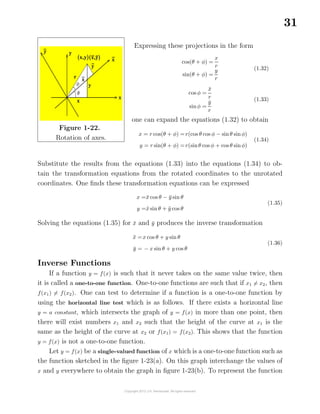
= lim
h→0
v(x)
u(x + h) − u(x)
h
− u(x)
v(x + h) − v(x)
h
v(x + h)v(x)
=
v(x) lim
h→0
u(x + h) − u(x)
h
− u(x) lim
h→0
v(x + h) − v(x)
h
lim
h→0
v(x + h)v(x)
or
dy
dx
=
d
dx
u(x)
v(x)
=
v(x)u (x) − u(x)v (x)
v2(x)
, where v2
(x) = [v(x)]2
This result is known as the quotient rule for differentiation.
A special case of the above result is the differentiation formula
d
dx
v(x)−1
=
d
dx
1
v(x)
=
−1
[v(x)]2
dv
dx
=
−1
[v(x)]2
v (x) (2.8)
Example 2-7. If y =
3x2
+ 8
x3 − x2 + x
, then find
dy
dx
Solution
Using the derivative of a quotient property one finds
dy
dx
=
d
dx
3x2
+ 8
x3 − x2 + x
=
(x3
− x2
+ x) d
dx (3x2
+ 8) − (3x2
+ 8) d
dx (x3
− x2
+ x)
(x3 − x2 + x)2
=
(x3
− x2
+ x)(6x) − (3x2
+ 8)(3x2
− 2x + 1)
(x3 − x2 + x)2
=
−3x4
− 21x2
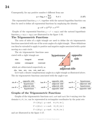
+ 16x − 8
(x3 − x2 + x)2
Differentiation of a Composite Function
If y = y(u) is a function of u and u = u(x) is a function of x, then the derivative
of y with respect to x equals the derivative of y with respect to u times the derivative
of u with respect to x or
dy
dx
=
d
dx
y(u) =
dy
du
du
dx
= y (u)u (x) (2.9)](https://image.slidesharecdn.com/calculusvolume-1-160216221448/85/Calculus-volume-1-106-320.jpg)
![99
This is known as the composite function rule for differentiation or the chain rule
for differentiation. Note that the prime notation always denotes differentiation with
respect to the argument of the function. For example z (ξ) =
dz
dξ
.
Proof
If y = y(u) is a function of u and u = u(x) is a function of x, then make note of
the fact that if x changes to x + ∆x, then u changes to u + ∆u and ∆u → 0 as ∆x → 0.
Hence, if ∆u = 0, one can use the identity
∆y
∆x
=
∆y
∆u
·
∆u
∆x
together with the limit theorem for products of functions, to obtain
dy
dx
= lim
∆x→0
∆y
∆x
= lim
∆u→0
∆y
∆u
· lim
∆x→0
∆u
∆x
=
dy
du
·
du
dx
= y (u)u (x)
which is known as the chain rule for differentiation.
An alternative derivation of this rule makes use of the definition of a derivative
given by equation (2.2). If y = y(u) is a function of u and u = u(x) is a function of x,
then one can write
dy
dx
= lim
h→0
y(x + h) − y(x)
h
= lim
h→0
y(u(x + h)) − y(u(x))
h
(2.10)
In equation (2.10) make the substitutions u = u(x) and ξ = u(x+h) and write equation
(2.10) in the form
dy
dx
= lim
ξ→u
y(ξ) − y(u)
(ξ − u)
·
(ξ − u)
h
dy
dx
= lim
ξ→u
y(ξ) − y(u)
ξ − u
· lim
h→0
u(x + h) − u(x)
h
dy
dx
=
dy
du
·
du
dx
= y (u)u (x)
Here the chain rule is used to differentiate a function of a function. For example, if
y = f(g(x)) is a function of a function, then make the substitution u = g(x) and write
y = f(u), then by the chain rule
dy
dx
=
dy
du
du
dx
= f (u)u (x) = f (u)g (x) (2.11)
The derivative of a function u = u(x) raised to a power n, n an integer, equals the
power times the function to the one less power times the derivative of the function or
d
dx
[u(x)n
] = nu(x)n−1 du
dx
= nu(x)n−1
u (x) (2.12)](https://image.slidesharecdn.com/calculusvolume-1-160216221448/85/Calculus-volume-1-107-320.jpg)
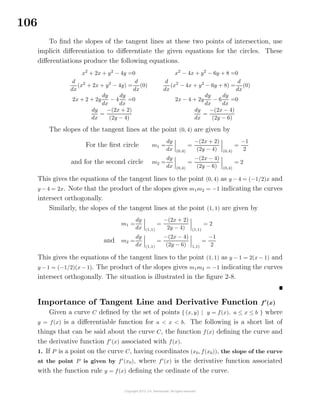
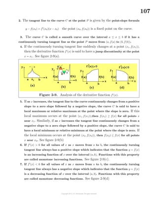
![108
Rolle’s Theorem4
If y = f(x) is a function satisfying (i) it is continuous
for all x ∈ [a, b] (ii) it is differentiable for all x ∈ (a, b) and
(iii) f(a) = f(b), then there exists a number c ∈ (a, b) such
that f (c) = 0.
This result is known as Rolle’s theorem. If y = f(x) is a
constant, the theorem is true so assume y = f(x) is different
from a constant. If the slope f (x) is always positive or
always negative for a ≤ x ≤ b, then f(x) would be either
continuously increasing or continuously decreasing between
the endpoints x = a and x = b and so it would be impossible
for y = f(x) to have the same value at both endpoints.
This implies that in order for f(a) = f(b) the derivative function f (x) must change
sign as x moves from a to b. If the derivative function changes sign it must pass
through zero and so one can say there exists at least one number x = c where f (c) = 0.
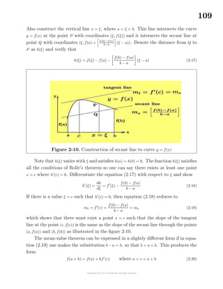
The Mean-Value Theorem
If y = f(x) is a continuous function for x ∈ [a, b] and is differentiable so that
f (x) exists for x ∈ (a, b), then there exists at least one number x = c ∈ (a, b) such that
the slope mt of the tangent line at (c, f(c)) is the same as the slope ms of the secant
line passing through the points (a, f(a)) and (b, f(b)) or
mt = f (c) =
f(b) − f(a)
b − a
= ms a < c < b
This result is known as the mean-value theorem and its implications are illustrated
in the figure 2-10.
Proof
A sketch showing the secant line and tangent line having the same slope is given
in the figure 2-10. In this figure note the secant line passing through the points
(a, f(a)) and (b, f(b)) and verify that the equation of this secant line is given by the
point-slope formula
y − f(a) =
f(b) − f(a)
b − a
(x − a)
4
Michel Rolle (1652-1719) A French mathematician. His name is pronounced “Roll”.](https://image.slidesharecdn.com/calculusvolume-1-160216221448/85/Calculus-volume-1-116-320.jpg)
![111
Cauchy’s Generalized Mean-Value Theorem
Let f(x) and g(x) denote two functions which are continuous on the interval [a, b].
Assume the derivatives f (x) and g (x) exist and do not vanish simultaneously for all
x ∈ [a, b] and that g(b) = g(a). Construct the function
y(x) = f(x)[g(b) − g(a)] − g(x)[f(b) − f(a)] (2.24)
and note that y(a) = y(b) = f(a)g(b) − f(b)g(a) and so all the conditions exist such that
Rolle’s theorem can be applied to this function. The derivative of the function given
by equation (2.24) is
y (x) = f (x)[g(b) − g(a)] − g (x)[f(b) − f(a)]
and Rolle’s theorem states that there must exist a value x = c satisfying a < c < b
such that
y (c) = f (c)[g(b) − g(a)] − g (c)[f(b) − f(a)] = 0 (2.25)
By hypothesis the quantity g(b) − g(a) = 0 and g (c) = 0, for if g (c) = 0, then equation
(2.25) would require that f (c) = 0, which contradicts our assumption that the deriva-
tives f (x) and g (x) cannot be zero simultaneously. Rearranging terms in equation
(2.25) gives Cauchy’s generalized mean-value theorem that f(x) and g(x) must satisfy
f(b) − f(a)
g(b) − g(a)
=
f (c)
g (c)
, a < c < b (2.26)
Note the special case g(x) = x reduces equation (2.26) to the form of equation (2.19).
Derivative of the Logarithm Function
Assume b > 0 is constant and y = y(x) = logb x. Use the definition of a derivative
and write
dy
dx
= y (x) = lim
∆x→0
y(x + ∆x) − y(x)
∆x
dy
dx
= y (x) = lim
∆x→0
logb(x + ∆x) − logb(x)
∆x
and use the properties of logarithms to write](https://image.slidesharecdn.com/calculusvolume-1-160216221448/85/Calculus-volume-1-119-320.jpg)
![114
Note the exponential function y = ex
is the only function equal to its own derivative.
Often times the exponential function y = ex
is expressed using the notation y = exp(x).
This is usually done whenever the exponent x is replaced by some expression difficult
to typeset as an exponent. Also note that the functions y = ex
and y = lnx are inverse
functions having the property that
eln x
= x for x > 0 and ln(ex
) = x for all values of x
If u = u(x), then a generalization of the above results is obtained using the chain
rule for differentiation. These generalizations are
d
dx
(bu
) =
d
du
(bu
) ·
du
dx
or
d
dx
(bu
) = (ln b) · bu
·
du
dx
and
d
dx
(eu
) =
d
du
(eu
) ·
du
dx
or
d
dx
(eu
) = eu
·
du
dx
(2.41)
Because the exponential function y = eu
is easy to differentiate, many differentiation
problems are converted to this form. For example, writing y = bx
= ex ln b
, then
dy
dx
=
d
dx
(bx
) =
d
dx
ex ln b
= ex ln b d
dx
[x ln b]
which simplifies to the result given by equation (2.39).
In differential notation, one can write
d eu
=eu
du
d au
=au
ln a du
d
au
ln a
=au
du, 0 < a < 1 or a > 1
(2.42)
Example 2-14. The differentiation formula
d
dx
xn
= nxn−1
was derived for n an
integer. Show that for x > 0 and r any real number one finds that
d
dx
xr
= rxr−1
Solution Use the exponential function and write y = xr
as y = er ln x
, then
dy
dx
=
d
dx
er ln x
= er ln x d
dx
(r ln x) = xr r
x
= rxr−1](https://image.slidesharecdn.com/calculusvolume-1-160216221448/85/Calculus-volume-1-122-320.jpg)
![115
Example 2-15. If y = | sinx|, find dy
dx
Solution Use the exponential function and write y = | sinx| = eln | sin x|
, then
dy
dx
=
d
dx
eln | sin x|
=eln | sin x| d
dx
ln| sinx|
=| sinx|
1
sin x
d
dx
sin x =
| sinx|
sinx
cos x =
cos x if sin x > 0
− cos x if sin x < 0
Example 2-16. If y = xcos x
with x > 0, find dy
dx
Solution Write y = xcos x
as y = e(cos x) ln x
, then
dy
dx
=
d
dx
e(cos x) ln x
=e(cos x) ln x d
dx
[(cos x) lnx]
=xcos x
cos x ·
1
x
+ ln x · (− sinx)
=xcos x cos x
x
− (ln x)(sinx)
Example 2-17. The general power rule for differentiation is expressed
d
dx
u(x)r
= ru(x)r−1
du
dx
(2.43)
where r can be any real number. This is sometimes written as
d
dx
u(x)r
=
d
dx
er ln u(x)
=er ln u(x) d
dx
[r ln u(x)]
=u(x)r
· r
1
u(x)
du
dx
=ru(x)r−1 du
dx
(2.44)
which is valid whenever u(x) = 0 with ln | u(x) | and u(x)r
well defined.](https://image.slidesharecdn.com/calculusvolume-1-160216221448/85/Calculus-volume-1-123-320.jpg)
![116
Example 2-18. The exponential function can be used to differentiate the
general power function y = y(x) = u(x)v(x)
, where u = u(x) > 0 and u(x)v(x)
is well
defined. One can write y = u(x)v(x)
= ev(x) ln u(x)
and by differentiation obtain
dy
dx
=
d
dx
ev(x) ln u(x)
=ev(x) ln u(x)
·
d
dx
[v(x) lnu(x)]
=u(x)v(x)
· v(x)
1
u(x)
du
dx
+
dv
dx
· ln u(x)
Derivative and Continuity
If a function y = f(x) is such that both the function f(x) and its derivative f (x)
are continuous functions for all values of x over some interval [a, b], then the function
y = f(x) is called a smooth function and its graph is called a smooth curve. A smooth
function is characterized by an unbroken curve with a continuously turning tangent .
Example 2-19.
(a) The function y = f(x) = x2
− 4 has the deriva-
tive dy
dx
= f (x) = 2x which is everywhere contin-
uous and so the graph is called a smooth curve.
(b) The function
y = f(x) = 2 + exp
1
3
ln | 2x − 3 | = 2 + (|2x − 3|)1/3
has the derivative
dy
dx
= e
1
3 ln|2x−3|
·
2
3(2x − 3)
which has a discontinuity in its derivative at the point x = 3/2 and so the curve is
not a smooth curve.
Maxima and Minima
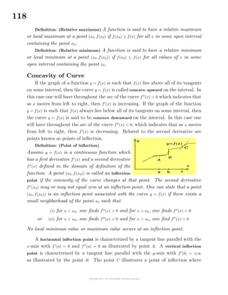
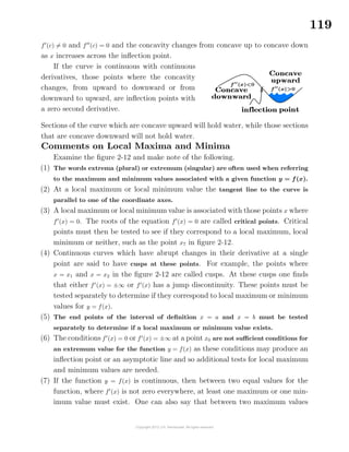
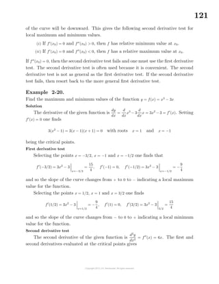
Examine the curve y = f(x) illustrated in the figure 2-12 which is defined and
continuous for all values of x satisfying a ≤ x ≤ b. Start at the point x = a and move
along the x-axis to the point b examining the heights of the curve y = f(x) as you
move left to right.](https://image.slidesharecdn.com/calculusvolume-1-160216221448/85/Calculus-volume-1-124-320.jpg)
![120
there is at least one minimum value or between two minimum values there is at
least one maximum value.
(8) In the neighborhood of a local maximum value, as x increases the function in-
creases, then stops changing and starts to decrease. Similarly, in the neighbor-
hood of a local minimum value, as x increases the function decreases, then stops
changing and starts to increase. In terms of a particle moving along the curve,
one can say that the particle change becomes stationary at a local maximum or
minimum value of the function. The terminology of finding stationary values of
a function is often used when referring to maximum and minimum problems.
First Derivative Test
The first derivative test for extreme values of a function tests the slope of the
curve at near points on either side of a critical point. That is, to test a given func-
tion y = f(x) for maximum and minimum values, one first calculates the derivative
function f (x) and then solves the equation f (x) = 0 to find the critical points. If x0
is a root of the equation f (x) = 0, then f (x0) = 0 and then one must examine how
f (x) changes as x moves from left to right across the point x0.
Slope Changes in Neighborhood of Critical Point
If the slope f (x) changes from
(i) + to 0 to −, then a local maximum occurs at the critical point.
(ii) − to 0 to +, then a local minimum occurs at the critical point.
(iii) + to 0 to +, then a point of inflection is said to exist at the critical point.
(iv) − to 0 to −, then a point of inflection is said to exist at the critical point.
Given a curve y = f(x) for x ∈ [a, b], the values of f(x) at the end points where
x = a and x = b must be tested separately to determine if they represents relative or
absolute extreme values for the function. Also points where the slope of the curve
changes abruptly, such as the point where x = x1 in figure 2-12, must also be tested
separately for local extreme values of the function.
Second Derivative Test
The second derivative test for extreme values of a function y = f(x) assumes that
the second derivative f (x) is continuous in the neighborhood of a critical point.
One can then say in the neighborhood of a local minimum value the curve will be
concave upward and in the neighborhood of a local maximum value the concavity](https://image.slidesharecdn.com/calculusvolume-1-160216221448/85/Calculus-volume-1-128-320.jpg)
![127
one critical point as y varies from 0 to h, since the area is zero at the end points
where y = 0 and y = h, the Rolle’s theorem implies there must be a maximum value
somewhere between. That is, if the area is a continuous function of y and A increases
as y increases from 0, then the only way for A to return to zero is for it to reach a
maximum value, stop and then return to zero.
Logarithmic Differentiation
Whenever one is confronted with functions which are represented by complicated
products and quotients such as
y = f(x) =
x2
√
3 + x2
(x + 4)1/3
or functions of the form y = f(x) = u(x)v(x)
, where u = u(x) and v = v(x) are complicated
functions, then it is recommended that you take logarithms before starting the
differentiation process. For example, to differentiate the function y = f(x) = u(x)v(x)
,
first take logarithms to obtain
ln y = ln u(x)v(x)
which simplifies to ln y = v(x) lnu(x)
The right-hand side of the resulting equation is a product function which can then
be differentiated. Differentiating both sides of the resulting equation, one finds
d
dx
lny =
d
dx
[v(x) lnu(x)] = v(x)
d
dx
ln u(x) + lnu(x)
d
dx
v(x)
1
y
·
dy
dx
=v(x)
1
u(x)
du(x)
dx
+ ln u(x) ·
dv(x)
dx
Solve this equation for the derivative term to obtain
dy
dx
= y · v(x)
1
u(x)
du(x)
dx
+ ln u(x) ·
dv(x)
dx
(2.46)
where y can be replaced by u(x)v(x)
.](https://image.slidesharecdn.com/calculusvolume-1-160216221448/85/Calculus-volume-1-135-320.jpg)
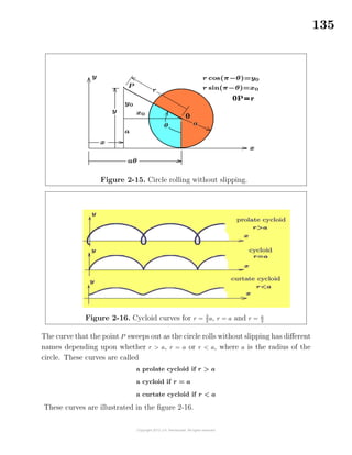
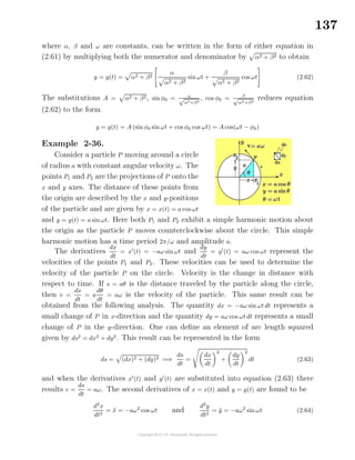
![136
To construct a tangent line to some point (x0, y0) on one of the cycloids, one must
be able to find the slope of the curve at this point. Using chain rule differentiation
one finds
dy
dθ
=
dy
dx
dx
dθ
or
dy
dx
=
dy
dθ
dx
dθ
, where
dx
dθ
= a − r cos θ and
dy
dθ
= r sin θ
The point (x0, y0) on the cycloid corresponds to some value θ0 of the parameter. The
slope of the tangent line at this point is given by
mt =
dy
dx
=
r sin θ
a − r cos θ θ=θ0
and the equation of the tangent line at this point is y − y0 = mt(x − x0).
Simple Harmonic Motion
If the motion of a particle or center of mass of a body can be described by either
of the equations
y = y(t) = A cos(ωt − φ0) or y = y(t) = A sin(ωt − φ0) (2.61)
where A, ω and φ0 are constants, then the particle or body is said to undergo a
simple harmonic motion. This motion is periodic with least period T = 2π/|ω|. The
amplitude of the motion is |A| and the quantity φ0 is called a phase constant or phase
angle.
Note 1: By changing the phase constant, one of the equations (2.61) can be trans-
formed into the other. For example,
A sin(ωt − φ0) = A cos [(ωt − φ0) − π/2] = A cos(ωt − θ0), θ0 = φ0 + π/2
and similarly
A cos(ωt − φ0) = A sin [(ωt − φ0) − π/2] = A sin(ωt − θ0), θ0 = φ0 + π/2
Note 2: Particles having the equation of motion
y = y(t) = α sinωt + β cos ωt](https://image.slidesharecdn.com/calculusvolume-1-160216221448/85/Calculus-volume-1-144-320.jpg)
![146
Now use the results from the equations (2.81) to show
sinh(x + y) =
1
2
[( coshx + sinhx)( coshy + sinhy) − ( coshx − sinhx)( coshy − sinhy)]
which when expanded simplifies to the desired result.
Replacing y by −y in the equations (2.83) produces the difference expansions
sinh(x − y) = sinhx coshy − coshx sinhy
cosh(x − y) = coshx coshy − sinhx sinhy
tanh(x − y) =
tanhx − tanhy
1 − tanhx tanhy
(2.84)
Substituting y = x in the equations (2.83) produces the results
sinh(2x) =2 sinhx coshx
cosh(2x) = cosh2
x + sinh2
y = 2 cosh2
x − 1 = 1 + 2 sinh2
x
tanh(2x) =
2 tanhx
1 + tanh2x
(2.85)
It is left for the exercises to verify the additional relations
sinhx + sinhy =2 sinh
x + y
2
cosh
x − y
2
coshx + coshy =2 cosh
x + y
2
cosh
x − y
2
tanhx + tanhy =
sinh(x + y)
coshx coshy
(2.86)
sinhx − sinhy =2 cosh
x + y
2
sinh
x − y
2
coshx − coshy =2 sinh
x + y
2
sinh
x − y
2
tanhx − tanhy =
sinh(x − y)
coshx coshy
(2.87)
sinh
x
2
=
1
2
( coshx − 1)
cosh
x
2
=
1
2
( coshx + 1)
tanh
x
2
=
coshx − 1
sinhx
=
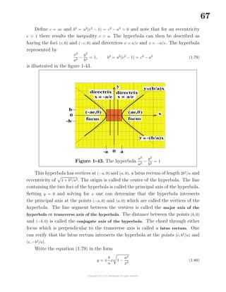
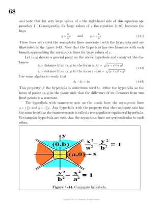
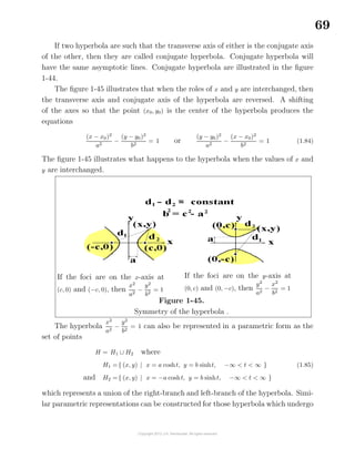
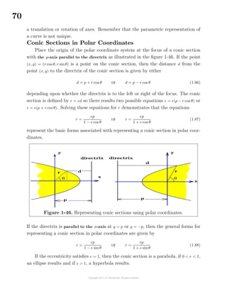
sinhx
coshx + 1
(2.88)](https://image.slidesharecdn.com/calculusvolume-1-160216221448/85/Calculus-volume-1-154-320.jpg)
![147
Euler’s Formula
Sometime around the year 1790 the mathematician Leonhard Euler13
discovered
the following relation
eix
= cos x + i sin x (2.89)
where i is an imaginary unit with the property i2
= −1. This formula is known as
Euler’s formula and is one of the most important formulas in all of mathematics.
The Euler formula can be employed to make a connection between the trigonometric
functions and the hyperbolic functions.
In order to prove the Euler formula given by equation (2.89) the following result
is needed.
If a function f(x) has a derivative f (x) which is everywhere zero within an
interval, then the function f(x) must be a constant for all values of x within the
interval.
The above result can be proven using the mean-value theorem considered earlier.
If f (c) = 0 for all values c in an interval and x1 = x2 are arbitrary points within the
interval, then the mean-value theorem requires that
f (c) =
f(x2) − f(x1)
x2 − x1
= 0
This result implies that f(x1) = f(x2) for all values x1 = x2 in the interval and hence
f(x) must be a constant throughout the interval.
To prove the Euler formula examine the function
F(x) = (cos x − i sinx)eix
, i2
= −1 (2.90)
where i is an imaginary unit, which is treated as a constant. Differentiate this
product and show
d
dx
F(x) = F (x) =(cos x − i sinx)eix
i + (− sinx − i cos x)eix
F (x) = [i cos x + sin x − sinx − i cos x] eix
= 0
(2.91)
Since F (x) = 0 for all values of x, then one can conclude that F(x) must equal a
constant for all values of x. Substituting the value x = 0 into equation (2.90) gives
F(0) = (cos 0 − i sin0)ei0
= 1
13
Leonhard Euler (1707-1783) A famous Swiss mathematician.](https://image.slidesharecdn.com/calculusvolume-1-160216221448/85/Calculus-volume-1-155-320.jpg)
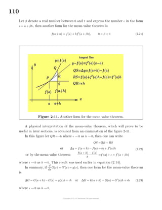
![155
The chain rule for differentiation can be used to generalize this result to
d
dx
sech−1
u =
−1
u
√
1 − u2
du
dx
, 0 < u < 1
If the lower half of the hyperbolic secant curve is used, then the sign of the above
result must be changed.
Differentiation of the logarithmic functions which define the inverse hyperbolic
functions, one obtains the results
d
dx
coth−1
u =
−1
u2 − 1
du
dx
, u2
> 1
d
dx
sech−1
u =
−1
u 1 + u2
du
dx
, sech−1
u > 0, 0 < u < 1
1
u 1 + u2
du
dx
, sech−1
u < 0, 0 < u < 1
d
dx
csch−1
u =
−1
u 1 + u2
du
dx
, u > 0
1
u 1 + u2
du
dx
, u < 0
(2.107)
Some additional relations involving the inverse hyperbolic functions are the fol-
lowing.
sinh−1
x = tanh−1 x
√
x2 + 1
sinh−1
x = ± cosh−1
x2 + 1
tanh−1
x = sinh−1 x
√
1 − x2
, |x| < 1
sinh−1
x = − i sin−1
(ix)
cosh−1
x = ± i cos−1
x
tanh−1
x = − i tan−1
(ix)
Example 2-47. As an exercise study Mercator pro-
jections and conformal mappings and show projections of
point P using line from 0 to A gives y2 latitude which dis-
torts map shape and distances and projections of point P
using the line C to B also distorts shapes and distances.
Show the correct conformal projection is y between y1 and
y2 such that dy
dθ
= sec θ and
y = ln[sec θ + tan θ] = tanh−1
[sin θ]](https://image.slidesharecdn.com/calculusvolume-1-160216221448/85/Calculus-volume-1-163-320.jpg)
![157
Table of Differentials
d(c u) = c du
d(u + v) = du + dv
d(u + v + w) = du + dv + dw
d(u v) = u dv + v du
d(u v w) = u v dw + u dv w + du v w
d
u
v
=
v du − u dv
v2
d (un
) = nun−1
du
d sin u = cos u du
d cos u = − sin u du
d tan u = sec2
u du
d cot u = − csc2
u du
d sec u = sec u tan u du
d csc u = − csc u cot u du
d (uv
) = v uv−1
du + un
(ln u) dv
d (uu
) = uu
(1 + ln u) du
d (eu
) = eu
du
d (bu
) = bu
(ln b) du
d(ln u) =
1
u
du
d(logb u) =
1
u
(logb e) du
d sin−1
u = (1 − u2
)−1/2
du
d cos−1
u = − (1 − u2
)−1/2
du
d tan−1
u = (1 + u2
)−1
du
d cot−1
u = − (1 + u2
)−1
du
d sec−1
u =
1
u
(u2
− 1)1/2
du
d csc−1
u = −
1
u
(u2
− 1)−1/2
du
All angles in first quadrant.
d sinhu = coshu du
d coshu = sinhu du
d tanhu = sech2
u du
d cothu = − csch2
u du
d sechu = − sechu tanhu du
d cschu = − cschu cothu du
d sinh−1
u = (u2
+ 1)−1/2
du
d cosh−1
u = (u2
− 1)−1/2
du
d tanh−1
u = (1 − u2
)−1
du
d coth−1
u = − (u2
− 1)−1
du
d sech−1
u = −
1
u
(1 − u2
)−1/2
du
d csch−1
u = −
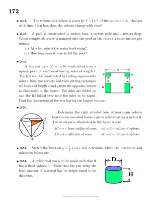
1
u
(u2
+ 1)−1/2
du
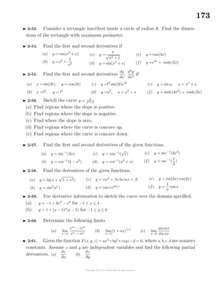
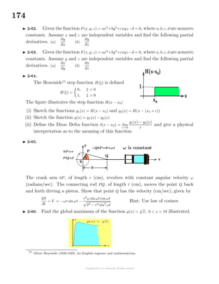
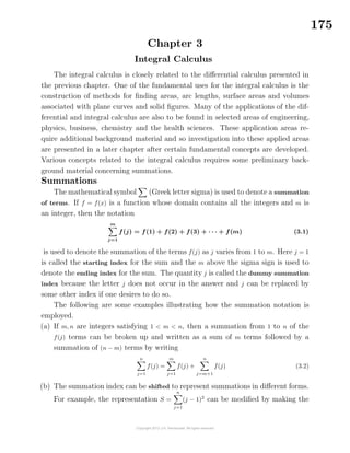
d(xy) =xdy + y dx
d(
x
y
) =
y dx − xdy
y2
d(
x2
+ y2
2
) =xdx + y dy
d(
y
x
) =
xdy − y dx
x2
d[tan−1
(
y
x
)] =
xdy − y dx
x2 + y2](https://image.slidesharecdn.com/calculusvolume-1-160216221448/85/Calculus-volume-1-165-320.jpg)
![159
Higher partial derivatives are defined as a derivative of a lower ordered derivative.
For example, The second partial derivatives of u = u(x, y) are defined
∂2
u
∂x2
=
∂
∂x
∂u
∂x
,
∂2
u
∂y2
=
∂
∂y
∂u
∂y
The second derivatives
∂2
u
∂x ∂y
=
∂
∂x
∂u
∂y
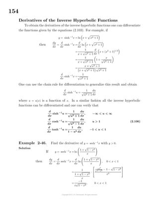
,
∂2
u
∂y ∂x
=
∂
∂y
∂u
∂x
are called
mixed partial derivatives. If both the function u = u(x, y) and its first ordered partial
derivatives are continuous functions, then the mixed partial derivatives are equal to
one another, in which case it doesn’t matter as to the order of the differentiation
and consequently
∂2
u
∂x ∂y
=
∂2
u
∂y ∂x
.
Total Differential
If u = u(x, y) is a continuous function of two variables, then as x and y change,
the change in u is written
∆u = u(x + ∆x, y + ∆y) − u(x, y)
Add and subtract the term u(x, y + ∆y) to the change in u and write
∆u = [u(x + ∆x, y + ∆y] − u(x, y + ∆y)] + [u(x, y + ∆y) − u(x, y)]
which can also be expressed in the form
∆u =
u(x + ∆x, y + ∆y) − u(x, y + ∆y)
∆x
∆x +
u(x, y + ∆y) − u(x, y)
∆y
∆y (2.108)
Now use the mean-value theorem on the terms in brackets to show
u(x + ∆x, y + ∆y) − u(x, y + ∆y)
∆x
=
∂u
∂x
+ 1
u(x, y + ∆y) − u(x, y)
∆y
=
∂u
∂y
+ 2
(2.109)
where 1 approaches zero as ∆x → 0 and 2 approaches zero as ∆y → 0. One can then
express the change in u as
∆u =
∂u
∂x
∆x +
∂u
∂y
∆y + 1 ∆x + 2 ∆y (2.110)
Define the differentials dx = ∆x and dy = ∆y and write the change in u as
∆u =
∂u
∂x
dx +
∂u
∂y
dy + 1 dx + 2 dy (2.111)](https://image.slidesharecdn.com/calculusvolume-1-160216221448/85/Calculus-volume-1-167-320.jpg)
![160
Define the total differential of u as
du =
∂u
∂x
dx +
∂u
∂y
dy (2.112)
and note the total differential du differs from ∆u by an infinitesimal of higher order
than dx or dy because 1 and 2 approach zero as ∆x → 0 and ∆y → 0. The total
differential du, given by equation (2.112) is sometimes called the principal part in
the change in u.
Notation
Partial derivatives are sometimes expressed using a subscript notation. Some
examples of this notation are the following.
∂u
∂x
=ux
∂u
∂y
=uy
∂2
u
∂x2
=uxx
∂2
u
∂x ∂y
=uxy
∂2
u
∂y2
=uyy
∂3
u
∂x3
=uxxx
∂3
u
∂x2∂y
=uxxy
∂3
u
∂x∂y2
=uxyy
∂3
u
∂y3
=uyyy
In general, if f = f(x, y) is a function of x and y and m = i + j is an integer, then
∂m
f
∂xi∂yj
is the representation of a mixed partial derivative of f.
Differential Operator
If u = u(x, y) is a function of two variables, then the differential of u is defined
du =
∂u
∂x
dx +
∂u
∂y
dy (2.113)
and if the variables x = x(t) and y = y(t) are functions of t, then u becomes a function
of t with derivative
du
dt
=
∂u
∂x
dx
dt
+
∂u
∂y
dy
dt
(2.114)
This is obtained by dividing both sides of equation (2.113) by dt. One can think of
equation (2.114) as defining the differential operator
d[ ]
dt
=
∂[ ]
∂x
dx
dt
+
∂[ ]
∂y
dy
dt
(2.115)
where the quantity to be substituted inside the brackets can be any function of x
and y where both x and y are functions of another variable t.](https://image.slidesharecdn.com/calculusvolume-1-160216221448/85/Calculus-volume-1-168-320.jpg)
![162
the planes x = x0 = a constant and y = y0 = a constant cut the surface f = f(x, y) in
one-dimensional curves. One can examine these one-dimensional curves for local
maximum and minimum values. For example, consider the curves defined by
Cx = { (x, y0, f) | f = f(x, y0) } Cy = { (x0, y, f) | f = f(x0, y)}
These curves have tangent lines with the slope of the tangent line to the curve Cx
given by ∂f
∂x
y=y0
= fx(x, y0) and the slope of the tangent line to the curve Cy given
by ∂f
∂y
x=x0
= fy(x0, y). At a local maximum or minimum value these slopes must be
zero. Consequently, one can say that a necessary condition for the point (x0, y0) to
corresponds to a local maximum or minimum value for f is that the conditions
∂f
∂x (x0,y0)
= fx(x0, y0) = 0 and
∂f
∂y (x0,y0)
= fy(x0, y0) = 0 simultaneously.
These are necessary conditions for an extreme value but they are not sufficient
conditions. The problem of determining a sufficient condition for an extreme value
will be considered in a later chapter and it will be shown that
If the function f = f(x, y) and its derivatives fx, fy, fxx, fxy, fyy exist and are
continuous at the point (x0, y0), then for f = f(x, y) to have an extreme value at
the point (x0, y0) the conditions
∂f
∂x (x0,y0)
= fx(x0, y0) = 0 and
∂f
∂y (x0,y0)
= fy(x0, y0) = 0
together with the condition fxx(x0, y0)fyy(x0, y0) − [fxy(x0, y0)]2
> 0 that must be
satisfied. One can then say
f(x0, y0) is a relative maximum value if fxx(x0, y0) < 0
f(x0, y0) is a relative minimum value if fxx(x0, y0) > 0
Implicit Differentiation
If F(x, y, . . ., z) is a continuous function of n−variables with continuous partial
derivatives, then the total differential of F is given by
dF =
∂F
∂x
dx +
∂F
∂y
dy + · · · +
∂F
∂z
dz (2.119)](https://image.slidesharecdn.com/calculusvolume-1-160216221448/85/Calculus-volume-1-170-320.jpg)
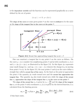
![166
2-13. Find the first and second derivatives of the following functions.
(a) y =
1
t
e−3t
(b) y =
1
x
1 − x2
(c) y = te−3t
(d) y = x
√
4 + 3 sinx
(e) y =
x
(x − a)(x − b)
(f) y =
1
x2 + a2
2-14. Find the first derivative dy
dx
and second derivative d2
y
dx2 associated with the
given parametric curve.
(a) x = a cos t, y = b sint
(b) x = 4 cos t, y = 4 sint
(c) x = 3t2
, y = 2t
(d) x = at, y = bt2
(e) x = a cosht, y = b sinht
(f) x = sin(3t + 4), y = cos(5t + 2)
2-15. Differentiate the given functions.
(a) y = x sin(4x2
)
(b) y = x2
e−3x
(c) y = xe−x
(d) y = cos(4x2
)
(e) y = x2
ln(3x), x > 0
(f) y = x2
tan(3x)
(g) y = ln(3x + 4) sin(x2
)
(h) y = ln(x2
+ x) cos(x2
)
(i) y = tan x sec x
2-16. Differentiate the given functions.
(a) y =
sin x
x
(b) y =
cos x
x
(c) y =
√
x + 1
x
(d) y =
x
√
x + 1
(e) y =
x
(1 + x2)3/2
(f) y =
(1 + x2
)3/2
x
(g) y = x2
ln(x2
)
(h) y = sin(x2
) ln(x3
)
(i) y = sin(x2
) cos(x2
)
2-17. Find the first and second derivatives of the given functions.
(a) y = x +
1
x
(b) y = sin2
(3x)
(c) y =
x
x + 1
(d) y = x2
+ 2x + 3 +
4
x
(e) y = cos2
(3x)
(f) y = tan(2x)
(g) y = x sin x
(h) y = x2
cos x
(i) y = x cos(x2
)
2-18. Find the tangent line to the given curve at the specified point.
(a) y = x +
1
x
, at (1, 2) (b) y = sinx, at (π/4, 1/
√
2) (c) y = x3
, at (2, 8)
2-19. Show that Rolle’s theorem can be applied to the given functions. Find all
values x = c such that Rolle’s theorem is satisfied.
(a) f(x) = 2 + sin(2πx), x ∈ [0, 1] (b) f(x) = x +
1
x
, x ∈ [1/2, 2]](https://image.slidesharecdn.com/calculusvolume-1-160216221448/85/Calculus-volume-1-174-320.jpg)
![167
2-20. Sketch the given curves and where appropriate describe the domain of the
function, symmetry properties, x and y−intercepts, asymptotes, relative maximum
and minimum points, points of inflection and how the concavity changes.
(a) y = x +
1
x
(b) y =
x
x + 1
(c) y = x4
− 6x2
(d) y = (x − 1)2
(x − 4)
(e) y = sinx + cos x
(f) y = x4
+ 12x3
+ 1
2-21. If f (x) = lim
h→0
f(x + h) − f(x)
h
(a) Show that f (x) = lim
h→0
f(x + 2h) − 2f(x + h) + f(x)
h2
(b) Substitute f(x) = x3
into the result from part (a) and show both sides of the
equation give the same result.
(c) Substitute f(x) = cos x into the result from part (a) and show both sides of the
equation give the same result. Hint: Use L´Hˆopital’s rule with respect to the
variable h.
2-22. Find the local maximum and minimum values associated with the given
curves.
(a) y = x2
− 4x + 3
(b) y =
x2
− x + 1
x2 + 1
(c) y =
2
x2 + 4
(d) y = −5 − 48x + x3
(e) y = sin x, all x
(f) y = cos x, all x
(g) y = sin(2πx), all x
(h) y = cos(2πx), all x
(i) y =
3
5 − 4 cos x
, x ∈ [−16, 16]
2-23. Find the absolute maximum and absolute minimum value of the given
functions over the domain D.
(a) y = f(x) = x2
+
2
x
, D = { x | x ∈ [1/2, 2] }
(b) y = f(x) =
x
x + 1
, D = { x | x ∈ [1, 2] }
(c) y = f(x) = sinx + cos x, D = { x | x ∈ [0, 2π] }
(d) y = f(x) =
x
1 + x2
, D = { x | x ∈ [−2, 2] }
2-24. Show that the given functions satisfy the conditions of the mean-value
theorem. Find all values x = c such that the mean-value theorem is satisfied.
(a) f(x) = −4 + (x − 2)2
, x ∈ [2, 6] (b) f(x) = 4 − x2
, x ∈ [0, 2]
2-25. A wire of length = 4 + π is to be cut into two parts. One part is bent into
the shape of a square and the other part is bent into the shape of a circle. Determine
how to cut the wire so that the area of the square plus the area of the circle has a
minimum value?](https://image.slidesharecdn.com/calculusvolume-1-160216221448/85/Calculus-volume-1-175-320.jpg)
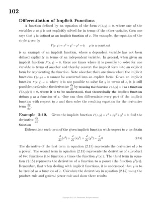
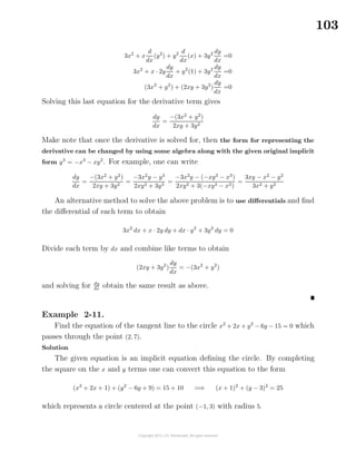
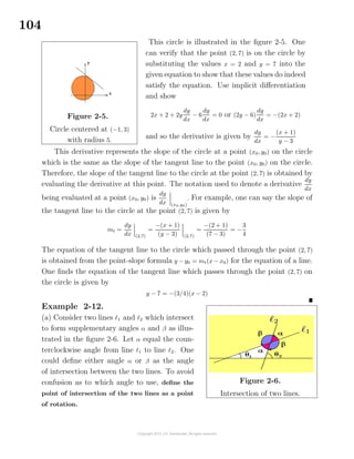
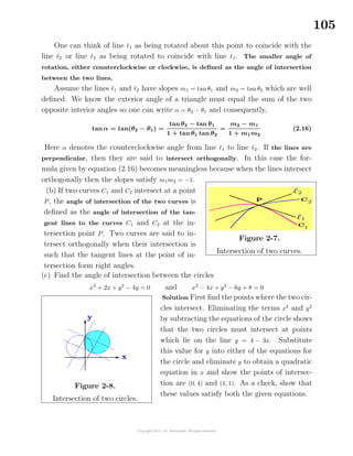
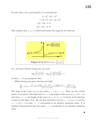
![168
2-26. A wire of length = 9 + 4
√
3 is to be cut into two parts. One part is bent
into the shape of a square and the other part is bent into the shape of an equilateral
triangle. Show how the wire is to be cut if the area of the square plus the area of
the triangle is to have a minimum value?
2-27. A wire of length = 9 +
√
3 is to be cut into two parts. One part is bent into
the shape of an equilateral triangle and the other part is bent into the shape of a
circle. Show how the wire is to be cut if the area of the triangle plus the area of the
circle is to have a minimum value?
2-28. Find the critical values and determine if the critical values correspond to a
maximum value, minimum value or neither.
(a) y = (x − 1)(x − 2)2
(b) y =
x2
− 7x + 10
x − 10
(c) y = f(x), where f (x) = x(x − 1)2
(x − 3)3
(d) y = f(x), where f (x) = x2
(x − 1)2
(x − 3)
2-29. Evaluate the given limits.
(a) lim
x→1
xn
− 1
x − 1
(b) lim
x→∞
1 +
1
x
x
(c) lim
x→0
ax2
+ bx
bx2 + ax
(d) lim
x→0
√
1 + x − 1
x
(e) lim
x→1
ln x
x2 − 1
(f) lim
x→0
ex
− e−x
sin x
(g) lim
x→0
ax
− 1
bx − 1
(h) lim
x→1
sinπx
x − 1
(i) lim
x→0
x − sinx
x2
2-30. Determine where the graph of the given functions are (a) increasing and
(b) decreasing. Sketch the graph.
(a) y = 8 − 10x + x2
(b) y = 3x2
− 5x + 2 (c) y = (x2
− 1)2
2-31. Verify the Leibnitz differentiation rule for the nth derivative of a product
of two functions, for the cases n = 1, n = 2, n = 3 and n = 4.
Dn
[u(x)v(x)] = Dn
[uv] =
n
i=0
n
i
Dn−i
u Di
v
Dn
[uv] =
n
0
(Dn
u) v +
n
1
Dn−1
u Dv +
n
2
Dn−2
u D2
v + · · · +
n
n
uDn
v
where
n
m
=
n!
m!(n − m)!
are the binomial coefficients. The general case can be
proven using mathematical induction.](https://image.slidesharecdn.com/calculusvolume-1-160216221448/85/Calculus-volume-1-176-320.jpg)
![177
is known as an arithmetic series with a called the first term, d called the common
difference between successive terms, = a + (n − 1)d is the last term and n is the
number of terms. Reverse the order of the terms in equation (3.6) and write
S = (a + (n − 1)d) + (a + (n − 2)d) + · · · + (a + d) + a (3.7)
and then add the equations (3.6) and (3.7) on a term by term basis to show
2S = n[a + a + (n − 1)d] = n(a + ) (3.8)
Solving equation (3.8) for S one finds the sum of an arithmetic series is given by
S =
n−1
j=0
(a + jd) =
n
2
(a + ) = n
a +
2
(3.9)
which says the sum of an arithmetic series is given by the number of terms multiplied
by the average of the first and last terms of the sum.
If f(x) = arx
, with a and r nonzero constants, the sum S =
n−1
j=0
f(j) =
n−1
j=0
arj
or
S =
n−1
j=0
f(j) =
n−1
j=0
arj
= a + ar + ar2
+ ar3
+ · · · + arn−1
(3.10)
is known as a geometric series, where a is the first term of the sum, r is the common
ratio of successive terms and n is the number of terms in the summation. Multiply
equation (3.10) by r to obtain
rS = ar + ar2
+ ar3
+ · · · + arn−1
+ arn
(3.11)
and then subtract equation (3.11) from equation (3.10) to show
(1 − r)S = a − arn
or S =
a − arn
1 − r
(3.12)
If |r| < 1, then rn
→ 0 as n → ∞ and in this special case one can write
S∞ = lim
n→∞
n−1
j=0
arj
= lim
n→∞
a − arn
1 − r
=
a
1 − r
, |r| < 1 (3.13)](https://image.slidesharecdn.com/calculusvolume-1-160216221448/85/Calculus-volume-1-185-320.jpg)
![181
The symbol is called an integral sign and is sometimes replaced by the words,
“The function whose differential is”. The symbol x used in the indefinite integral
given by equation (3.20) is called a dummy variable of integration. It can be replaced
by some other symbol. For example,
if
d
dξ
G(ξ) = g(ξ) then g(ξ) dξ = G(ξ) + C (3.21)
where C is called a constant of integration.
Example 3-2.
The following integrals occur quite often and should be memorized.
If
d
dx
x = 1, then 1 dx = x + C
If
d
dx
x2
= 2x, then 2x dx = x2
+ C
If
d
dx
x3
= 3x2
, then 3x2
dx = x3
+ C
If
d
dx
xn
= nxn−1
, then nxn−1
dx = xn
+ C
If
d
du
um+1
m + 1
= um
, then um
du =
um+1
m + 1
+ C
If
d
dt
sint = cos t, then cos t dt = sin t + C
If
d
dt
cos t = − sint, then sin t dt = − cos t + C
or dx = x + C
or d(x2
) = x2
+ C
or d(x3
) = x3
+ C
or d(xn
) = xn
+ C
or d
um+1
m + 1
=
um+1
m + 1
+ C
or d(sint) = sin t + C
or − d(cos t) = − cos t + C
Properties of the Integral Operator
If f(x) dx = F(x) + C, then
d
dx
F(x) = f(x)
That is, to check that the integration performed is accurate, observe that one must
have the derivative of the particular integral F(x) always equal to the integrand
function f(x).
If f(x) dx = F(x) + C, then
αf(x) dx = α f(x) dx = α [F(x) + C] = αF(x) + K
for all constants α. Here K = αC is just some new constant of integration. This
property is read, “The integral of a constant times a function equals the constant
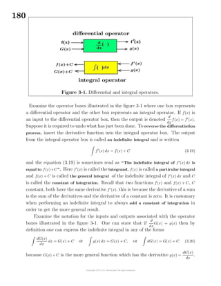
times the integral of the function.”](https://image.slidesharecdn.com/calculusvolume-1-160216221448/85/Calculus-volume-1-189-320.jpg)
![182
If f(x) dx = F(x) + C and g(x) dx = G(x) + C, then
[f(x) + g(x)] dx = f(x) dx + g(x) dx = F(x) + G(x) + C
This property states that the integral of a sum is the sum of the integrals. The
constants C in each of the above integrals are not the same constants. The symbol
C represents an arbitrary constant and all C s are not the same. That is, the sum of
arbitrary constants is still an arbitrary constant. For example, examine the state-
ment that the integral of a sum is the sum of the integrals. If for i = 1, 2, . . ., m you
know fi(x) dx = Fi(x) + Ci, where each Ci is an arbitrary constant, then one could
add a constant of integration to each integral and write
[f1(x) + f2(x) + · · · + fm(x)] dx = f1(x) dx + f2(x) dx + · · · + fm(x) dx
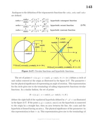
=[F1(x) + C1] + [F2(x) + C2] + · · · + [Fm(x) + Cm]
=F1(x) + F2(x) + · · · + Fm(x) + C
All the arbitrary constants of integration can be combined to form just one arbitrary
constant of integration.
Notation
There are different notations for representing an integral. For example, if
d
dx
F(x) = f(x), then dF(x) = f(x) dx and dF(x) = f(x) dx = F(x) + C or
f(x) dx =
d
dx
F(x) dx = dF(x) = F(x) + C (3.22)
Examine equation (3.22) and observe dF(x) = F(x) + C. One can think of the
differential operator d and the integral operator as being inverse operators of each
other where the product of operators d produces unity. These operators are
commutative so that d also produces unity. For example,
d f(x) dx = d[F(x) + C] = dF(x) + dC = f(x) dx
Some additional examples of such integrals are the following.](https://image.slidesharecdn.com/calculusvolume-1-160216221448/85/Calculus-volume-1-190-320.jpg)
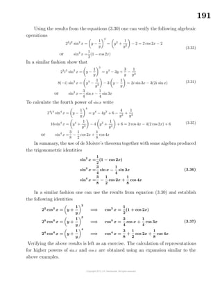
![194
to obtain the product relations
sinmx sin nx =
1
2
[cos(m − n)x − cos(m + n)x]
sinmx cos nx =
1
2
[sin(m − n)x + sin(m + n)x]
cos mx cos nx =
1
2
[cos(m − n)x + cos(m + n)x]
(3.39)
which, with proper scaling, reduce the above integrals to forms involving simple
integration of sine and cosine functions.
Example 3-11. Evaluate the integral I = sin 5x sin 3x dx
Solution Using the above trigonometric substitution one can write
I =
1
2
[cos 2x − cos 8x] dx =
1
4
cos 2x 2dx −
1
16
cos 8x 8dx
to obtain, after proper scaling of the integrals,
I = sin 5x sin 3x dx =
1
4
sin 2x −
1
16
sin 8x + C
Special Trigonometric Integrals
Examining the previous tables of derivatives and integrals one finds that integrals
of the trigonometric functions tan x, cot x, sec x and csc x are missing. Let us examine
the integration of each of these functions.
Integrals of the form tan u du
To evaluate this integral express it in the form dw
w
as this is a form which can
be found in the previous tables. Note that
tan u du =
sin u
cos u
du = −
d(cos u)
cos u
= − ln| cos u| + C
An alternative approach is to write
tanu du =
sec u tanu
sec u
du =
d(sec u)
sec u
= ln | secu| + C
Therefore one can write
tan u du = − ln | cos u| + C = ln | sec u| + C](https://image.slidesharecdn.com/calculusvolume-1-160216221448/85/Calculus-volume-1-202-320.jpg)
![200
which can be easily integrated to obtain I = 9 ln|x − 1| + ln |x2
+ 2x + 5| + lnK. This
result can be further simplified and one finds I = ln K(x − 1)9
(x2
+ 2x + 5) where K
is an arbitrary constant.
Case 4 The denominator Q(x) has one or more quadratic factors, some of which
are repeated quadratic factors. In this case, for each repeated quadratic factor
(ax2
+ bx + c)k
there corresponds a sum of partial fractions of the form
A1x + B1
ax2 + bx + c
+
A2x + B2
(ax2 + bx + c)2
+ · · · +
Akx + Bk
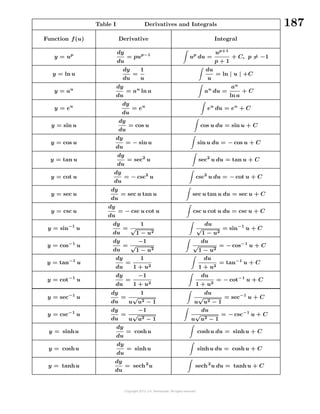
(ax2 + bx + c)k
where A1, B1, . . . , Ak, Bk are constants to be determined.
Before giving an example of this last property let us investigate the use of partial
fractions to evaluate special integrals which arise during the application of case 4
above. These special integrals will then be summarized in a table for later reference.
Integrals of the form
dx
β2 − x2
, where x < β.
Use partial fractions and write
dx
β2 − x2
=
1
2β
1
β + x
+
1
β − x
dx
=
1
2β
[ln|β + x| − ln|β − x|] + C
so that
dx
β2 − x2
=
1
2β
ln
β + x
β − x
+ C = −
1
β
tanh−1 x
β
+ C, x < β
See for example the previous result of equation (2.103) with x replaced by x/β.
Integrals of the form
dx
x2 − β2
, where x > β.
Use partial fractions and show
dx
x2 − β2
=
1
2β
1
x − β
−
1
x + β
dx
=
1
2β
[ln|x − β| − ln|x + β|] + C
This can be simplified to one of the forms
dx
x2 − β2
=
1
2β
ln
x − β
x + β
+C = −
1
β
coth−1
x
β
+C = −
1
β
tanh−1
β
x
+C, x > β
Here the previous results from equation (2.103) have been used to produce the
alternative form above.](https://image.slidesharecdn.com/calculusvolume-1-160216221448/85/Calculus-volume-1-208-320.jpg)
![201
Integrals of the form
dx
x2 + β2
Make the substitution x = β tan u with dx = β sec2
u du to obtain
dx
x2 + β2
=
β sec2
u du
β2(tan2
u + 1)
=
1
β
du =
1
β
u + C
where u = tan−1 x
β
. Therefore one can write
dx
x2 + β2
=
1
β
tan−1 x
β
+ C
or by constructing a right triangle representing the substitution, one can write the
equivalent forms
dx
x2 + β2
=
1
β
cos−1 β
x2 + β2
+ C =
1
β
sec−1 x2 + β2
β
+ C
Integrals of the form
dx
(x2 + β2)2
Make the trigonometric substitution x = β tanθ with dx = β sec2
θ dθ and show
dx
(x2 + β2)2
=
β sec2
θ dθ
β4(tan2
θ + 1)2
=
1
β3
sec2
θ
sec4 θ
dθ =
1
β3
cos2
θ dθ
=
1
2β3
(1 + cos 2θ) dθ =
1
2β3
θ +
1
2
sin2θ =
1
2β3
[θ + sin θ cos θ]
Using back substitution representing θ in terms of x one finds
dx
(x2 + β2)2
=
1
2β3
tan−1 x
β
+
βx
x2 + β2
+ C
where C is a general constant of integration added to make the result more general.
Integrals of the form
dx
ax2 + bx + c
Integrals having the form I =
dx
Q(x)
, where Q(x) = ax2
+ bx + c is a quadratic
factor, can be evaluated if one first performs a completing the square operation on
the quadratic term. One finds that either
ax2
+ bx + c =a x +
b
2a
2
+
4ac − b2
4a2
where 4ac − b2
> 0
or ax2
+ bx + c =a x +
b
2a
2
−
b2
− 4ac
4a2
where b2
− 4ac > 0](https://image.slidesharecdn.com/calculusvolume-1-160216221448/85/Calculus-volume-1-209-320.jpg)
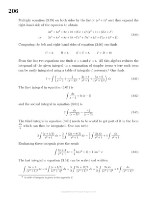
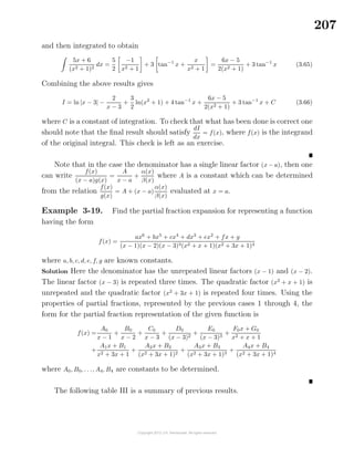
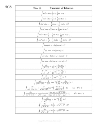
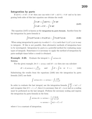
![211
x2
sin nx dx = x2 − cos nx
n
− 2x
− cosnx
n
dx
Use scaling and apply integration by parts on the last integral, with U = 2x and
dV = −cos nx
n dx, to obtain
2x
− cos nx
n
dx = 2x
− sinnx
n2
− 2
− sinnx
n2
dx
The last integral can be scaled and integrated. One finds that the last integral
becomes
2
− sinnx
n2
dx =
2
n3
cos nx
Back substitution gives the results
x2
sinnx dx = x2 − cosnx
n
− 2x
− sinnx
n2
+
2
n3
cos nx + C
where C is a general constant of integration which can be added at the end of any
indefinite integral.
Reduction Formula
The use of the integration by parts formula U dV = UV − V dU to evaluate
an integral gives a representation of a first integral in terms of a second integral.
Sometimes, when an integration by parts is performed on the second integral, one
finds that it can be reduced to a form of the first integral. When this happens one
can usually obtain a general formula, known as a reduction formula, for evaluating
the first and sometimes the second integral.
Example 3-22. Evaluate the integral Im = sinm
x dx where m is a positive
integer.
Solution Write the integral as Im = sinm−1
x sin x dx and use integration by parts
with
U = sinm−1
x
dU =(m − 1) sinm−2
x cos x dx
dV = sin x dx
V = − cos x
to obtain
Im = − sinm−1
x cos x + (m − 1) sinm−2
x cos2
x dx
Im = − sinm−1
x cos x + (m − 1) sinm−2
x(1 − sin2
x) dx
Im = − sinm−1
x cos x + (m − 1) [Im−2 − Im]
and using algebra one can solve for Im to obtain](https://image.slidesharecdn.com/calculusvolume-1-160216221448/85/Calculus-volume-1-219-320.jpg)
![214
Figure 3-2. Area under curve and partitioning the interval [a, b] into n-parts.
The curve y = f(x) is assumed to be such that y > 0 and continuous for all x ∈ [a, b].
To find an approximation to the area desired, construct a series of rectangles as
follows.
(1) Divide the interval [a, b] into n-parts by defining a step size ∆x =
b − a
n
and then
define the points
x0 =a
x1 =a + ∆x = x0 + ∆x
x2 =a + 2∆x = x1 + ∆x
...
...
xi =a + i∆x = xi−1 + ∆x
...
...
xn =a + n∆x = a + n
(b − a)
n
= b = xn−1 + ∆x
(3.80)
This is called partitioning the interval (a, b) into n-parts.
(2) Select arbitrary points ti, within each ∆x interval, such that xi−1 ≤ ti ≤ xi for all
values of i ranging from i = 1 to i = n. Then for all values of i ranging from 1 to
n construct rectangles of height f(ti) with the bottom corners of the rectangle
touching the x-axis at the points xi−1 and xi as illustrated in the figure 3-2.
(3) The area of the ith rectangle is denoted Ai=(height)(base), where the height of
the rectangle is f(ti) and its base is ∆xi = xi − xi−1. The sum of all the rectangles
is given by St
n =
n
i=1
Ai =
n
i=1
f(ti) ∆xi which is called the Riemann3
sum for the
3
Georg Friedrich Bernhard Riemann (1826-1866) A German mathematician.](https://image.slidesharecdn.com/calculusvolume-1-160216221448/85/Calculus-volume-1-222-320.jpg)
![215
function y = f(x). The resulting sum is determined by the partition constructed.
This Riemannian sum represents an approximation to the area under the curve.
This approximation gets better as each ∆xi gets smaller.
Define the limit of the Riemann sum
lim
n→∞
St
n = lim
n→∞
n
i=1
Ai = lim
∆x→0
n→∞
n
i=1
f(ti)∆xi =
b
a
f(x) dx, xi−1 ≤ ti ≤ xi (3.81)
where the quantity on the right-hand side of equation (3.81) is called the definite
integral from a to b of f(x) dx and the quantity on the left-hand side of equation (3.81)
is the limit of the sum of rectangles as ∆x tends toward zero. The notation for the
definite integral from a to b of f(x) dx has the physical interpretation illustrated in
the figure 3-3.
Figure 3-3. Mnemonic device for determining area under curve.
The quantity f(x) dx = dA is to represent an element of area which is a rectangle
positioned a distance x from the origin, having height f(x) and base dx. The integral
sign is an elongated S to remind you that rectangles are being summed and
the lower limit a and upper limit b on the integral sign is to remind you that the
summation of rectangles is a limiting process taking place between the limits x = a
and x = b.
Observe that if F(x) is a differentiable function which is continuous over the
interval [a, b] and F(x) is selected as a particular integral of f(x), then one can write
dF(x)
dx
= F (x) = f(x), or one can write the indefinite integral
f(x) dx =
dF(x)
dx
dx = dF(x) = F(x) + C](https://image.slidesharecdn.com/calculusvolume-1-160216221448/85/Calculus-volume-1-223-320.jpg)
![216
It will now be demonstrated that any function F(x) which is a particular integral
of f(x) can be used to evaluate the definite integral
b
a
f(x) dx. To accomplish this
graph the function y = F(x), satisfying F (x) = f(x), between the values x = a and
x = b and then partition the interval [a, b] into n-parts in the same way as for the
original function y = f(x). Apply the mean-value theorem for derivatives to the points
(xi−1, F(xi−1)) and (xi, F(xi)) associated with the ith ∆x interval of the curve y = F(x).
In using the mean-value theorem make special note that the function F(x) is related
to f(x) by way of differentiation so that F (x) = f(x) is the slope of the curve y = F(x)
at the point x. One can then calculate the slope of the secant line through the points
(xi−1, F(xi−1)) and (xi, F(xi)) as
ms =
∆F
∆x
=
F(xi) − F(xi−1)
xi − xi−1
The mean-value theorem says there must exist a point ci satisfying xi−1 ≤ ci ≤ xi,
such that the slope of the tangent line to the curve y = F(x), at the point x = ci,
is the same as the slope of the secant line. By our choice of F(x), the slope of the
tangent line to F(x) at the point x = ci is given by f(ci) since F (x) = f(x). Therefore,
one can write
F(xi) − F(xi−1)
xi − xi−1
= f(ci) or F(xi) − F(xi−1) = f(ci)∆xi, ∆xi = xi − xi−1 (3.82)
This mean-value relationship can be applied to each ∆x interval for all values of i
ranging from 1 to n.
Make note of the fact the points ti, i = 1, . . ., n, used to evaluate the definite
integral in equation (3.81) were not specified. They were arbitrary points satisfying
xi−1 ≤ ti ≤ xi for each value of the index i ranging from 1 to n. Note the values ci,
i = 1, . . ., n which satisfy the mean-value equation (3.82) are special values. Suppose
one selects for equation (3.81) the values ti = ci as i ranges from 1 to n. In this
special case the summation given by equation (3.81) becomes
Sc
n =
n
i=1
f(ci)∆xi = [F(x1) − F(x0)] + [F(x2) − F(x1)] + · · · + [F(xn) − F(xn−1)]
n
i=1
f(ci)∆xi =F(xn) − F(x0) = F(b) − F(a)
(3.83)
Observe that the summation of terms on the right-hand side of equation (3.83) is a
telescoping sum and can be written as](https://image.slidesharecdn.com/calculusvolume-1-160216221448/85/Calculus-volume-1-224-320.jpg)
![217
[F(x1) − F(x0)] + [F(x2) − F(x1)]
+ [F(x3) − F(x2)] + [F(x4) − F(x3)]
...
+ [F(xn−1) − F(xn−2)] + [F(xn) − F(xn−1)] = F(xn) − F(x0) = F(b) − F(a)
where as i ranges from 1 to n − 1, for each term F(xi) there is a −F(xi) and so these
terms always add to zero and what is left is just the last term minus the first term.
This result still holds as ∆x → 0 and so one can state that the area bounded by the
curve y = f(x), the x-axis, the lines x = a and x = b is given by the definite integral
b
a
f(x) dx = F(x)
b
a
= F(b) − F(a) (3.84)
where F(x) is any particular integral of f(x).
Observe that the constant of integration associated with the indefinite integral
can be omitted when dealing with definite integrals. If this constant were used,
then equation (3.84) would become [F(b) + C] − [F(a) + C] = F(b) − F(a) which is
the same result as given in equation (3.84). Also note that the name “definite
integral” indicates that the integral has a definite value of F(b) − F(a), which does
not contain the symbol x or the constant C. The symbol x is called a dummy variable
of integration in the definite integral and can be replaced by some other symbol.
The above result is a special case of the fundamental theorem of integral calculus.
Fundamental theorem of integral calculus
Let f(x) > 0 denote a continuous function over the interval a ≤ x ≤ b. Partition
the interval (a, b) into n subintervals [x0, x1], [x1, x2], . . ., [xi−1, xi], . . ., [xn−1, xn] which
may or may not be of equal length. Select an arbitrary point ti ∈ [xi−1, xi] for
i = 1, 2, . . ., n and construct the rectangles of height f(ti) and base ∆xi = xi −xi−1 with
Ai = f(ti)∆xi the area of the ith rectangle. A special case of the above situation is
illustrated in the figure 3-2.
Let An =
n
i=1 Ai =
n
i=1 f(ti)∆xi denote the Riemannian sum which equals the
sum of the areas of these rectangles and let F(x) denote any function which is
an integral of f(x) with the property F(x) = f(x) dx or
dF(x)
dx
= f(x). Then the
fundamental theorem of integral calculus can be expressed
lim
n→∞
An = limn→∞
∆x→0
n
k=1
f(tk)∆x =
b
a
f(x) dx = F(x)
b
a
= F(b) − F(a)](https://image.slidesharecdn.com/calculusvolume-1-160216221448/85/Calculus-volume-1-225-320.jpg)
![218
Since F (x) = f(x), the fundamental theorem of integral calculus is sometimes ex-
pressed in the form
b
a
F (x) dx = F(x)
x=b
x=a
= F(b) − F(a)
Note that the limiting summation of rectangles that represents the definite in-
tegral of f(x) from x = a to x = b has the same value no matter how the points ti are
selected inside the interval [xi−1, xi], for i = 1, 2, . . ., n. This is because of the continuity
of f(x) over the interval [a, b]. Recall that f(x) is a continuous function if for every 1
there exists a positive number δ1 such that
|f(ti) − f(ci)| < 1 whenever |ti − ci| < δ1 (3.85)
Suppose it is required that the condition given by (3.85) be satisfied for each value
i = 1, 2, . . ., n. If 1 =
(b − a)
, with as small as desired, and n is selected large enough
such that ∆x =
b − a
n
< δ1, then one can compare the two summations
St
n =
n
i=1
f(ti)∆xi and Sc
n =
n
i=1
f(ci)∆xi
One finds the absolute value of the difference of these sums satisfies
|St
n − Sc
n| =
n
i=1
[f(ti)∆xi − f(ci)∆xi] ≤
n
i=1
|f(ti) − f(ci)| ∆xi
For n large enough such that each ∆xi =
b − a
n
< δ1 for all values of the index i and
|f(ti) − f(ci)| < 1 for all values of the index i, then St
n − Sc
n ≤ n 1∆x = n
b − a
b − a
n
=
This states that the difference between the two sums St
n and Sc
n can be made as small
as desired for n large enough and in the limit these sums are the same. A similar
type of argument can be made for an arbitrary, unequally spaced, partitioning of
the interval [a, b].
Properties of the Definite Integral
1. If F (x) =
dF(x)
dx
= f(x), then the definite
integral
A(x) = F(x) − F(a) =
x
a
f(t) dt
represents the area under the curve y = f(t) be-
tween the limits t = a and t = x. Whenever the
upper or lower limit of integration involves the symbol x, then the dummy variable
of integration in the definite integral is usually replaced by a different symbol.](https://image.slidesharecdn.com/calculusvolume-1-160216221448/85/Calculus-volume-1-226-320.jpg)
![219
2. Differentiate the above result to show
dA(x)
dx
=
dF(x)
dx
=
d
dx
x
a
f(t) dt = f(x) (3.86)
This shows that to differentiate a definite integral with respect to x, where the
upper limit of integration is x and the lower limit of integration is a constant,
one obtains the integrand evaluated at the upper limit x.
3. If the direction of integration is changed, then the sign of the integral changes
a
b
f(x) dx = −
b
a
f(x) dx (3.87)
4. The interval of integration [a, b] can be broken up into smaller subintervals, say,
[a, ξ1], [ξ1, ξ2], [ξ2, b] and the integral written
b
a
f(x) dx =
ξ1
a
f(x) dx +
ξ2
ξ1
f(x) dx +
b
ξ2
f(x) dx (3.88)
5. Assume the curve y = f(x) crosses the x-axis at some point x = c between the
lines x = a and x = b, such that f(x) is positive for a ≤ x ≤ c and f(x) is negative
for c ≤ x ≤ b, then
c
a
f(x) dx represents a positive area
and the integral
b
c
f(x) dx represents a negative area.
The definite integral
b
a
f(x) dx represents the summation of the signed areas
above and below the x-axis. The integral
b
a
|f(x)| dx represents a summation of
positive areas.
6. The summation
n
i=1
f(ti) represents the sum of the heights associated with the
rectangles constructed in the figure 3-2, and the sum ¯y =
1
n
n
i=1
f(ti) represents
the average height of these rectangles. Using the equation (3.81) show that in
the limit as ∆x → 0 and using ∆xi =
b − a
n
, this average height can be represented
¯y = lim
∆x→0
n→∞
1
n
n
i=1
f(ti) = lim
∆x→0
n→∞
1
b − a
n
i=1
f(ti)∆xi =
1
b − a
b
a
f(x) dx](https://image.slidesharecdn.com/calculusvolume-1-160216221448/85/Calculus-volume-1-227-320.jpg)
![220
This states that the average value for the height of the curve y = f(x) between
the limits x = a and x = b is given by
Average height of curve = ¯y =
1
b − a
b
a
f(x) dx (3.89)
7. The integral of a constant times a function equals the constant times the integral
of the function or b
a
cf(x) dx = c
b
a
f(x) dx
8. Change of variables in a definite integral
Given an integral of the form I =
b
a
f(g(x)) g (x) dx it is customary to make the
substitution u = g(x) with du = g (x) dx. When this is done in a definite integral, then
the limits of integration must also be changed. Thus, when x = a, then u = g(a) and
when x = b, then u = g(b) so that if f(u) is well defined on the interval [g(a), g(b)], then
the given integral can be reduced to the form
I =
b
a
f(g(x)) g (x) dx =
g(b)
g(a)
f(u) du
9. Area between curves
Let y = f(x) and y = g(x) denote two curves which are continuous on the interval
[a, b] and assume that f(x) ≤ g(x) for all x ∈ [a, b], then one can state that
b
a
f(x) dx ≤
b
a
g(x) dx or
b
a
g(x) dx ≥
b
a
f(x) dx
Sketch the curves y = f(x), y = g(x), the lines x = a and x = b and sketch in a
rectangular element of area dA representative of all the rectangular elements being
summed to find the area bounded by the curves and the lines x = a and x = b. Note
that the element of area is given by
dA = (y of upper curve − y of lower curve) dx](https://image.slidesharecdn.com/calculusvolume-1-160216221448/85/Calculus-volume-1-228-320.jpg)
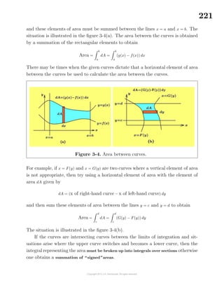
![222
Example 3-25. Consider the definite integral I =
π/6
0
sin 2x cos4
2x dx
Make the change of variable u = cos 2x with du = −2 sin2x dx. The new limits of
integration are found by substituting x = 0 and x = π/6 into the equation u = cos 2x
to obtain ua = cos 2x
x=0
= 1 and ub = cos 2x
x=π/6
=
1
2
. Here du = −2 sin2x dx
and so the given integral must be scaled. The scaled integral can then be written
I =
−1
2
π/6
0
(cos 2x)4
(−2 sin2x dx)
where now the substitutions for u, du and new limits on integrations can be performed
to obtain
I =
−1
2
1/2
1
u4
du =
1
2
1
1/2
u4
du =
1
2
u5
5
1
1/2
=
1
10
1 −
1
32
=
31
320
Example 3-26. Find the area between the curves y = sin x and y = cos x for
0 ≤ x ≤ π.
Solution
Sketch the given curves over the domain specified and show the curves intersect
where x = π/4. The given integral can then be broken up into two parts and one can
write
A1 =
π/4
0
[cos x − sin x] dx = sinx + cos x
π/4
0
=
√
2 − 1
A2 =
π
π/4
[sin x − cos x] dx = − cos x − sin x
π
π/4
= 1 +
√
2
The total area is then A1 + A2 = 2
√
2
A summation of the signed areas is given by
π
0
[cos x − sin x] dx = (
√
2 − 1) − (1 +
√
2) = −2 = A1 − A2
Example 3-27. Find the area of the triangle bounded by the x-axes, the line
y = h
b1
x and the line y = h − h
b2
(x − b1), where b = b1 + b2.](https://image.slidesharecdn.com/calculusvolume-1-160216221448/85/Calculus-volume-1-230-320.jpg)
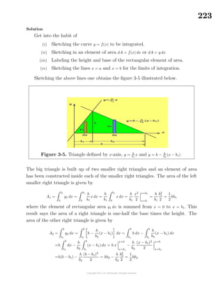
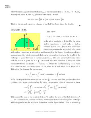
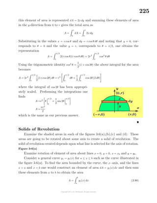
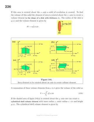
![228
The total volume is then given by a summation of these volume elements
V = π
b
a
[y2
0 − (y0 − y1(x))2
] dx
Figure 3-6(b)
Examine rotation of element of area about lines x = 0, y = 0, x = x0 and y = y0.
Examine the figure 3-6(b) and show that to determined the area bounded by the
curve x1 = x1(y), the y−axis and the lines y = α, y = β is obtained by a summation of
the area element dA = x1(y) dy from α to β. The total area is given by
A =
β
α
x1(y) dy
If the area is rotated about a line, then a solid of revolution is created. To find
the volume of the solid one can rotate the element of area about the line to create
an element of volume which can then be summed. Consider the element of area
illustrated as being rotated about the axes (i) the x−axis, (ii) the y−axis, (iii) the
line x = x0 and (iv) the line y = y0 to obtain respectively elements of volumes in the
shapes of (i)a cylindrical shell element, (ii) a disk element, (iii) a washer element and
(iv) another cylindrical shell element. Show these volume elements are given by
(i) dV = 2πyx1(y) dy
(ii) dV = πx2
1(y) dy
(iii) dV = π x2
0 − (x0 − x1(y))2
dy
(iv) dV = 2π(y0 − y)x1(y) dy
Figure 3-6(c)
Examine rotation of element of area about lines x = 0, y = 0, x = x0 and y = y0.
Examine the figure 3-6(c) and show the area bounded by the curves y1 = y1(x),
y2 = y2(x) and the lines x = a, x = b, is obtained by a summation of the area element
dA = [y1(x) − y2(x)] dx from a to b. This summation gives the total area as
A =
b
a
(y1(x) − y2(x)) dx
If this area is rotated about a line, then a solid of revolution is created. To find the
volume of the solid one can rotate the element of area about the same axis to create
an element of volume which can then be summed. Consider the element of area
being rotated about the axes (i) the x−axis, (ii) the y−axis, (iii) the line x = x0 and
(iv) the line y = y0 to obtain respectively elements of volumes in the shapes of (i) a
washer element, (ii) a cylindrical shell element, (iii) another cylindrical shell element
and (iv) another washer element. Show these volume elements can be represented
as follows.](https://image.slidesharecdn.com/calculusvolume-1-160216221448/85/Calculus-volume-1-236-320.jpg)
![229
(i) dV = π y2
2 (x) − y2
1 (x) dx
(ii) dV = 2πx[y1(x) − y2(x)] dx
(iii) dV = 2π(x0 − x)[y1(x) − y2(x)] dx
(iv) dV = π (y0 − y2(x))2
− (y0 − y1(x))2
dx
Figure 3-6(d)
Examine rotation of element of area about lines x = 0, y = 0, x = x0 and y = y0.
Examine the figure 3-6(d) and show the area bounded by the curves x1 = x1(y),
x2 = x2(y) and the lines y = α, y = β, is obtained by a summation of the area element
dA = [x1(y) − x2(y)] dy from α to β. This summation gives the total area
A =
β
α
[x1(y) − x2(y)] dy
If this area is rotated about a line, then a solid of revolution is created. The volume
associated with this solid is determined by a summation of an appropriate volume
elements. These volume elements can be determined by rotating the element of area
about the same line from which the solid was created.
Consider the element of area rotated about the lines (i) the x−axis, (ii) the
y−axis, (iii) the line x = x0 and (iv) the line y = y0 to obtain respectively elements
of volumes in the shapes of (i) a cylindrical shell element, (ii) a washer element,
(iii) another washer element and (iv) another cylindrical shell element. Show these
volume elements can be represented as follows.
(i) dV = 2πy[x1(y) − x2(y)] dy
(ii) dV = π x2
1(y) − x2
2(y) dy
(iii) dV = π (x0 − x2(y))2
− (x0 − x1(y))2
dy
(iv) dV = 2π(y0 − y)(x1(y) − x2(y)) dy
Example 3-29. Take the semi-circle
{ (x, y) | x = r cos θ, y = r sin θ, 0 ≤ θ ≤ π }
as defined in the previous example and rotate it about the x-axis to form a sphere.
The figure 3-7 will aid in visualizing this experiment.
Note that the vertical element of area when rotated becomes an element of
volume dV in the shape of a disk with radius y and thickness dx. The volume of this
disk is given by dV = πy2
dx and a summation of these volume elements from x = −r
to x = r gives
V =
r
−r
dV =
r
−r
πy2
dx](https://image.slidesharecdn.com/calculusvolume-1-160216221448/85/Calculus-volume-1-237-320.jpg)
![230
Making the same substitutions as in the previous example one finds
V =
0
π
π(r sinθ)2
(−r sin θ) dθ = πr3
π
0
sin3
θ dθ
Figure 3-7.
Semi-circle rotated about x-axis creating the volume element in shape of a disk.
Now use the trigonometric identity
sin3
θ =
1
4
(3 sinθ − sin 3θ)
and express the volume integral in the form of an integration of trigonometric func-
tions. After appropriate scaling, make use of the integration table to show that
V =
πr3
4
π
0
(3 sinθ − sin3θ) dθ =
πr3
4
3
π
0
sin θ dθ −
1
3
π
0
sin 3θ(3dθ)
V =
πr3
4
3(− cos θ)
π
0
−
1
3
(− cos 3θ)
π
0
=
πr3
4
−3(−1 − 1)] +
1
3
(−1 − 1)
V =
4
3
πr3
This shows the volume of the sphere of radius r is 4/3 times π times the radius cubed.
If the horizontal element of area illustrated in the example 3-24, is rotated about
the x-axis a cylindrical shell element results, like the one illustrated by equation
(3.92), but with x and y interchanged. The inner radius of the cylinder is y and the
outer radius is y + dy and the length of the cylinder is 2x. The element of volume is
given by
dV =π(length)[(outer radius)2
− (inner radius)2
]
dV =π(2x)[(y + dy)2
− y2
] = π(2x)[y2
+ 2y dy + (dy)2
− y2
]
dV =2π(2x)y dy + π(2x)(dy)2](https://image.slidesharecdn.com/calculusvolume-1-160216221448/85/Calculus-volume-1-238-320.jpg)
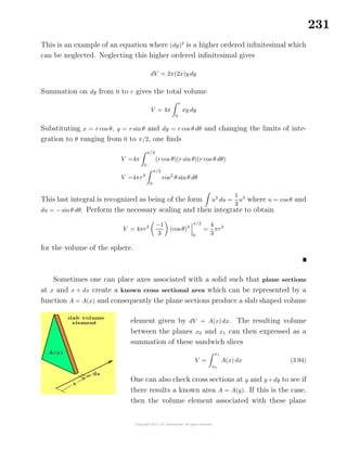
![232
slices are written dV = A(y) dy and the total volume between the planes y0 and y1 is
expressed as the summation
V =
y1
y0
A(y) dy (3.95)
Integration by Parts
Integration by parts associated with a definite integral has the form
b
a
u(x)v (x) dx =
b
a
d(u(x)v(x)) dx −
b
a
v(x)u (x) dx
b
a
u(x)v (x) dx =u(x)v(x)
x=b
x=a
−
b
a
v(x)u (x) dx
b
a
u(x)v (x) dx =u(b)v(b) − u(a)v(a) −
b
a
v(x)u (x) dx
(3.96)
Example 3-30. To integrate I =
T
0
te−st
dt let u = t with du = dt and dv = e−st
dt
with v = −1
s
e−st
, then the integration by parts formula gives
I =
T
0
te−st
dt =
−t
s
e−st
T
0
−
T
0
−1
s
e−st
dt =
−T
s
e−sT
−
1
s2
e−st
T
0
=
−T
s
e−sT
−
1
s2
[e−sT
− 1]
Example 3-31. Evaluate the integral J =
π/2
−π/2
x sin x dx
Solution Let U = x and dV = sin x dx giving dU = dx and V = − cos x, so that integration
by parts produces the result
J = −x cos x
π/2
−π/2
−
π/2
−π/2
− cos x dx = −
π
2
cos
π
2
+
−π
2
cos
−π
2
+ sinx
π/2
−π/2
= 2
Example 3-32. Evaluate the integral I =
b
a
x2
√
b − x dx, where a, b are constants
satisfying a < b.
Solution Use integration by parts with
u =x2
du =2x dx
dv =(b − x)1/2
dx
v = −
2
3
(b − x)3/2](https://image.slidesharecdn.com/calculusvolume-1-160216221448/85/Calculus-volume-1-240-320.jpg)
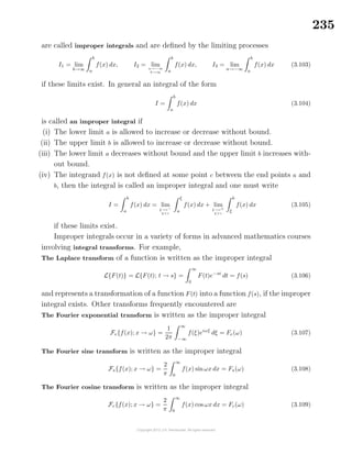
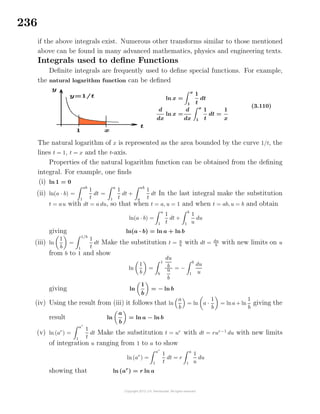
![238
Arc Length
Let y = f(x) denote a continuous curve for x ∈ [a, b] and consider the problem
of assigning a length to the curve y = f(x) between the points (a, f(a)) = P0 and
(b, f(b)) = Pn. Partition the interval [a, b] into n-parts by defining ∆x =
b − a
n
and
labeling the points
a = x0, x1 = x0 + ∆x, x2 = x1 + ∆x, . . ., xi = xi−1 + ∆x, . . ., xn = xn−1 + ∆x = b
as illustrated in the figure 3-9.
Label the points (xi, f(xi)) = Pi for i = 0, 1, 2, . . ., n and construct the line segments
Pi−1Pi for i = 1, 2, . . ., n. These line segments connect the points
(x0, f(x0)), (x1, f(x1)), (x2, f(x2)), . . ., (xi, f(xi)), . . ., (xn−1, f(xn−1)), (xn, f(xn))
in succession and form a polygonal line connecting the points (a, f(a)) and (b, f(b)).
Figure 3-9.
Approximation of arc length by summation of straight line segments.
The sum of these line segments can be represented
sn =
n
i=1
(xi − xi−1)2 + [f(xi) − f(xi−1)]2 =
n
i=1
1 +
f(xi) − f(xi−1)
∆xi
2
∆xi (3.115)
where ∆xi = xi −xi−1. This sum is an approximation to the length of the curve y = f(x)
between the points (a, f(a)) and (b, f(b)). This arc length approximation gets better
as ∆xi gets smaller or as n gets larger. If in the limit as n → ∞, the above sum exists](https://image.slidesharecdn.com/calculusvolume-1-160216221448/85/Calculus-volume-1-246-320.jpg)
![239
so that one can write s = lim
n→∞
sn, then the curve y = f(x) is said to be rectifiable.
The limiting value s is defined to be the arc length of the curve y = f(x) between the
end points (a, f(a)) and (b, f(b)). Here lim
∆x→0
f(xi) − f(xi−1)
∆xi
= f (xi) and the infinite sum
becomes a definite integral and so one can express the limiting value of the above
sum as
s =
b
a
1 + [f (x)]2 dx =
b
a
1 +
dy
dx
2
dx (3.116)
If x ∈ [a, b], then define the arc length s = s(x) of the curve y = f(x) between the points
(a, f(a)) and (x, f(x)) as
s = s(x) =
x
a
1 + [f (t)]2 dt (3.117)
and define the differential of arc length ds = s (x) dx. The element of arc length ds
can be determined from any of the following forms
ds = dx2 + dy2 = 1 +
dy
dx
2
dx =
dx
dy
2
+ 1 dy
ds =
dx
dt
2
+
dy
dt
2
dt = [x (t)]2 + [y (t)]2 dt
(3.118)
Example 3-33. Find the circumference of the circle defined by x = r cos θ,
y = r sin θ for 0 ≤ θ ≤ 2π, where r is a constant.
Solution
The element of arc length squared can be written
ds2
=dx2
+ dy2
or
ds = [x (θ)]2 + [y (θ)]2] dθ
Substituting in the derivatives
dx
dθ
= x (θ) = −r sin θ and
dy
dθ
= y (θ) = r cos θ, the element
of arc length is
ds = [−r sinθ]2 + [r cos θ]2 dθ = r sin2
θ + cos2 θ dθ = r dθ
and the total arc length is a summation of these elements
s = r
2π
0
dθ = r θ
2π
0
= 2π r](https://image.slidesharecdn.com/calculusvolume-1-160216221448/85/Calculus-volume-1-247-320.jpg)
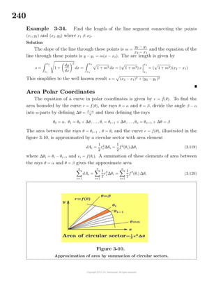
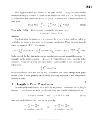
![242
and represent the total differentials in terms of the variables r and θ. Squaring and
adding these differentials one finds
ds2
= dx2
+ dy2
= dr2
+ r2
dθ2
(3.123)
as the representation for the arc length squared in polar coordinates. Other forms
for representing the element of arc length in polar coordinates are
ds =
dr
dθ
2
+ r2 dθ = 1 + r2
dθ
dr
2
dr = [r (t)]2 + r2[t][θ (t)]2 dt (3.124)
Example 3-36. Find the circumference of the circle r = 2r0 cos θ given in the
previous example.
Solution Here an element of arc length is given by the polar coordinate representation
ds =
dr
dθ
2
+ r2 dθ, where
dr
dθ
= −2r0 sinθ. Integration of the element of arc length
from 0 to π gives
s =
π
0
4r2
0 sin2
θ + 4r2
0 cos2 θ dθ = 2r0
π
0
dθ = 2r0θ
π
0
= 2πr0
Surface of Revolution
When a curve is revolved about the x or y-
axis a surface of revolution results. The problem
of determining the surface area of the resulting
surface of revolution is approached using the fol-
lowing arguments. First consider a right circular cone where the top has been cut
off. The resulting figure is called the frustum of a right circular cone. The top sur-
face is the shape of a circle with radius r1 and the bottom surface is a circle with
radius r2 > r1. The side surface has a slant height of length as illustrated in the
accompanying figure. The surface area associated with the side of this figure is given
by5
Side surface area = π(r1 + r2) (3.125)
5
How this result is derived can be found in example 3-38](https://image.slidesharecdn.com/calculusvolume-1-160216221448/85/Calculus-volume-1-250-320.jpg)
![243
Figure 3-11.
Arc length ds rotated about x-axis to form frustum of right circular cone.
Consider next the surface of revolution obtained when a curve y = f(x) is rotated
about the x-axis as illustrated in the figure 3-11. Let ds denote an element of arc
length in cartesian coordinates connecting the points (x, y) and (x + dx, y + dy) on the
curve and observe that when this element is rotated about the x-axis a frustum of
a right circular cone results. The radius of one circle is y and radius of the other
circle is y + dy. The element of surface area dS is the side surface area of the frustum
and given by equation (3.125) and so one can write
dS = π[y + (y + dy)] ds (3.126)
The product dy ds is an infinitesimal of the second order and can be neglected so
that the element of surface area can be written in the form
dS = 2πy ds (3.127)
By the fundamental theorem of integral calculus a summation of these surface el-
ements gives the total surface area of the surface of revolution. This total surface
area can be expressed in different forms depending upon the representation of the
arc length ds (See equations (3.118).) If y = y(x), then one can write
S =
b
a
2πy ds = 2π
b
a
y 1 +
dy
dx
2
dx (3.128)
In a similar fashion, a curve x = F(y), for c ≤ y ≤ d, rotated about the y-axis
would created a surface of revolution with surface area given by
S = 2π
d
c
x 1 +
dx
dy
2
dy (3.129)](https://image.slidesharecdn.com/calculusvolume-1-160216221448/85/Calculus-volume-1-251-320.jpg)
![245
Mean Value Theorems for Integrals
There are several mean value theorems associated with definite integrals which
can be found under the following names.
(i) The first mean value theorem for integrals. If f(x) is a continuous function for
a ≤ x ≤ b, then there is a point x = ξ1 ∈ [a, b] such that
b
a
f(x) dx = (b − a) f(ξ1) = (b − a)f(a + θ1(b − a)), 0 < θ1 < 1 (3.131)
(ii) The generalized first mean value theorem for integrals.
If both f(x) and g(x) are continuous functions for a ≤ x ≤ b and the function
g(x) does not change sign for x ∈ [a, b], then there exists a point x = ξ2 ∈ [a, b] such
that
b
a
f(x)g(x) dx = f(ξ2)
b
a
g(x) dx = f(a + θ2(b − a))
b
a
g(x) dx, 0 < θ2 < 1 (3.132)
(iii) Bonnet’s second mean value theorem for integrals.
If both f(x) and g(x) are continuous functions for a ≤ x ≤ b and the function g(x)
is a positive monotonic6
decreasing function, then there exists a point x = ξ3 ∈ [a, b]
such that b
a
f(x)g(x) dx = g(a)
ξ3
a
f(x) dx (3.133)
where ξ3 = a + θ3(b − a), for 0 < θ3 < 1. Alternatively, if g(x) is a positive monotonic
increasing function, then there exists a point x = ξ4 ∈ [a, b] such that
b
a
f(x)g(x) dx = g(b)
b
ξ4
f(x) dx (3.134)
where ξ4 = a + θ4(b − a), for 0 < θ4 < 1.
(iv) The generalized second mean value theorem for integrals.
If both f(x) and g(x) are continuous functions for a ≤ x ≤ b and the function
g(x) is a monotone increasing or monotone decreasing over the interval [a, b], then
there exists a point x = ξ5 ∈ [a, b] such that
b
a
f(x)g(x) dx = g(a)
ξ5
a
f(x) dx + g(b)
b
ξ5
f(x) dx (3.135)
where ξ5 = a + θ5(b − a), for 0 < θ5 < 1.
6
If f(x) is defined on an interval [a, b] and if f is such that whenever a < x1 < x2 < b, there results
f(x1) ≤ f(x2), then f is called a monotone increasing function over the interval [a, b]. If the inequality above is
reversed so that f(x1) ≥ f(x2), then f is called a monotone decreasing function over the interval [a, b].](https://image.slidesharecdn.com/calculusvolume-1-160216221448/85/Calculus-volume-1-253-320.jpg)
![246
Proof of Mean Value Theorems
If f(x) > 0 is a continuous function over the interval a ≤ x ≤ b, define the functions
G(x) =
x
a
g(t) dt,
G (x) =g(x),
H(x) =
x
a
f(t)g(t) dt,
H (x) =f(x)g(x),
P(x) =G(x)H(b) − G(b)H(x)
P (x) =G (x)H(b) − G(b)H (x)
and observe that P(a) = P(b) = 0 because G(a) = H(a) = 0 and the way P(x) is defined.
Consequently, it is possible to apply Rolle’s7
theorem which states that there must
exist a value x = ξ, for a < ξ < b, such that P (ξ) = 0. This requires
g(ξ)
b
a
f(t)g(t) dt − f(ξ)g(ξ)
b
a
g(t) dt = 0
which simplifies to give the generalized first mean value theorem for integrals
b
a
f(x)g(x) dx = f(ξ)
b
a
g(x) dx
Note the special case g(x) = 1 produces the first mean value theorem for integrals.
To prove Bonnet’s second mean value theorem, assume f(x) > 0 is a continuous
function for a ≤ x ≤ b and consider the cases where g(x) is monotone decreasing and
monotone increasing over the interval [a, b].
Case 1: Assume that g(x) is positive and monotone decreasing over the inter-
val [a, b]. Define the function φ(x) = g(a)
x
a
f(x) dx which is continuous over the
interval [a, b] and demonstrate φ(a) = 0 ≤
b
a
f(x)g(x) dx ≤ φ(b). An application
of the intermediate value theorem shows there exists a value x = ξ such that
φ(ξ) = g(a)
ξ
a
f(x) dx =
b
a
f(x)g(x) dx.
Case 2: Assume that g(x) is positive and monotone increasing over the interval
[a, b]. Define the function ψ(x) = g(b)
b
x
f(x) dx which is continuous over the in-
terval [a, b] and demonstrate ψ(b) = 0 ≤
b
a
f(x)g(x) dx ≤ ψ(a). An application of
the intermediate value theorem shows that there exists a value x = ξ such that
ψ(ξ) = g(b)
b
ξ
f(x) dx =
b
a
f(x)g(x) dx.
To prove the generalized second mean value theorem for integrals consider the
function F(x) =
x
a
f(u) du and then evaluate the integral
b
a
f(x)g(x) dx using integra-
tion by parts to show
b
a
f(x)g(x) dx = g(x)F(x)
b
a
−
b
a
F(x)g (x) dx = g(b)F(b) −
b
a
F(x)g (x) dx (3.136)
7
Michel Rolle (1652-1719) a French mathematician.](https://image.slidesharecdn.com/calculusvolume-1-160216221448/85/Calculus-volume-1-254-320.jpg)
![247
The last integral in equation (3.136) can be evaluated as follows. The assumption
that g(x) is a monotonic function implies that the derivative g (x) is of a constant
sign for x ∈ [a, b] so that by the generalized first mean value theorem for integrals the
equation (3.136) can be expressed in the form
b
a
f(x)g(x) dx =g(b)F(b) − F(ξ)
b
a
g (x) dx = g(b)F(b) − F(ξ)[g(b) − g(a)]
=g(a)F(ξ) + g(b)[F(b) − F(ξ)] = g(a)
ξ
a
f(x) dx + g(b)
b
ξ
f(x) dx
(3.137)
Differentiation of Integrals
The general Leibnitz formula for the differentiation of a general integral, where
both the lower and upper limits of integration are given by functions α(t) and β(t),
is given by the relation
d
dt
β(t)
α(t)
f(t, τ) dτ =
β(t)
α(t)
∂f(t, τ)
∂t
dτ + f(t, β(t))
dβ
dt
− f(t, α(t))
dα
dt
(3.138)
To derive the Leibnitz differentiation formula consider the following simpler exam-
ples.
Example 3-39. Show that
d
dx
x
a
f(t) dt = f(x) where a is a constant.
Solution Let F(x) =
x
a
f(t) dt and use the definition of a derivative to obtain
dF(x)
dx
= lim
∆x→0
F(x + ∆x) − F(x)
∆x
= lim
∆x→0
x+∆x
a
f(t) dt −
x
a
f(t) dt
∆x
= lim
∆x→0
1
∆x
x+∆x
x
f(t) dt
Apply the mean value theorem for integrals and show the above reduces to
dF(x)
dx
= F (x) = lim
∆x→0
1
∆x
f(x + θ ∆x) ∆x = f(x), where 0 < θ < 1
Consequently, one can write
d
dx
x
a
f(t) dt = f(x),
d
dβ
β
0
f(t) dt = f(β),
d
dα
α
0
f(t) dt = f(α)
Note that the above results imply that
d
dx
a
x
f(t) dt = −
d
dx
x
a
f(t) dt = −f(x).](https://image.slidesharecdn.com/calculusvolume-1-160216221448/85/Calculus-volume-1-255-320.jpg)
![248
Example 3-40. Show that
d
dx
β(x)
α(x)
f(t) dt = f(β(x))
dβ
dx
− f(α(x))
dα
dx
Solution Write the given integral in the form
d
dx
β(x)
α(x)
f(t) dt =
d
dx
0
α(x)
f(t) dt +
β(x)
0
f(t) dt =
d
dx
β(x)
0
f(t) dt −
α(x)
0
f(t) dt
and use chain rule differentiation employing the results from the previous example
to show
d
dx
β(x)
α(x)
f(t) dt =
d
dx
β(x)
0
f(t) dt −
α(x)
0
f(t) dt
=
d
dβ
β
0
f(t) dt
dβ
dx
−
d
dα
α
0
f(t) dt
dα
dx
d
dx
β(x)
α(x)
f(t) dt =f(β(x))
dβ
dx
− f(α(x))
dα
dx
Example 3-41.
Consider the function I = I(x, g(x), h(x)) defined by the integral
I = I(x, g, h) =
h(x)
g(x)
f(x, t) dt (3.139)
where the integrand is a function of both the variables x and t and the limits of
integration g and h are also functions of x. The integration is with respect to the
variable t and it is assumed that the integrand f is both continuous and differentiable
with respect to x. The differentiation of a function defined by an integral containing
a parameter x is given by the Leibnitz rule
dI
dx
= I (x) =
h(x)
g(x)
∂f(x, t)
∂x
dt + f(x, h(x))
dh
dx
− f(x, g(x))
dg
dx
. (3.140)
The above result follows from the definition of a derivative together with the use of
chain rule differentiation.
Consider first the special case of the integral I1(x) =
h
g
f(x, t) dt where g and h
are constants. Calculate the difference
I1(x + ∆x) − I1(x) =
h
g
[f(x + ∆x, t) − f(x, t)] dt
and then employ the mean value theorem with respect to the x-variable and write](https://image.slidesharecdn.com/calculusvolume-1-160216221448/85/Calculus-volume-1-256-320.jpg)
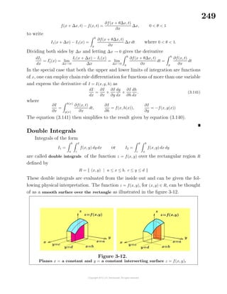
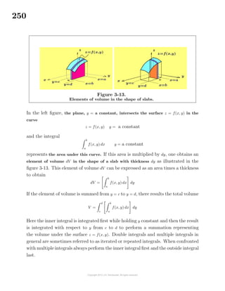
![251
In a similar fashion, the plane, x = a constant, intersects the surface z = f(x, y) in
the curve
z = f(x, y) x = a constant
so that the integral
d
c
f(x, y) dy x = a constant
represents the plane area under the curve. If the resulting area is multiplied by dx,
one obtains a volume element dV in the shape of a slab times a thickness dx. This
slab is given by
dV =
d
c
f(x, y) dy dx
If these volume elements are summed from x = a to x = b, then the resulting volume
under the surface is given by
V =
b
a
d
c
f(x, y) dy dx
Another way to interpret the previous double integrals is to first partition the
interval [a, b] into n parts by defining ∆x = b−a
n
and then partition the interval [c, d]
into m parts by defining ∆y = d−c
m
. One can then define the points
a =x0, . . ., xi = a + i∆x, . . .xn = a + n∆x = a + n
b − a
n
= b
c =y0, . . ., yj = c + j∆y, . . .ym = c + m∆y = c + m
d − c
m
= d
where i and j are integers satisfying 0 ≤ i ≤ n and 0 ≤ j ≤ m. One can then move to a
point (xi, yj) located within the rectangle R and construct a parallelepiped of height
f(xi, yj) and base with sides ∆xi = xi+1 − xi and ∆yj = yj+1 − yj as illustrated in the
figure 3-14.
Figure 3-14. Element of volume dV = f(x, y) dy dx](https://image.slidesharecdn.com/calculusvolume-1-160216221448/85/Calculus-volume-1-259-320.jpg)
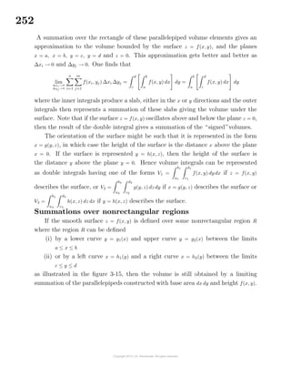
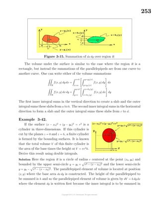
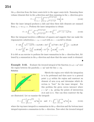
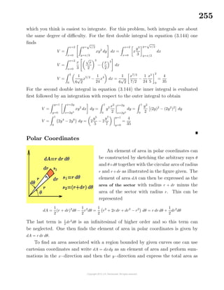
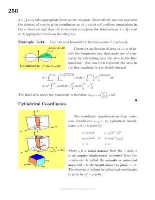
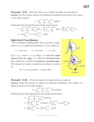
![258
Using Table of Integrals
The appendix C contains a table of integrals. In order to use these tables one
must sometimes make appropriate substitutions in order to convert an integral into
the proper form as given in the tables. For example, if it is required to evaluate the
integral
I =
e3x
dx
a + bex
where a and b are constants and you look for this integral in the table, you will not
find it. This is because the integral is listed under a different form. If you make the
substitution u = ex
with du = ex
dx The above integral can be written in the form
I =
u2
du
a + bu
where u = ex
which is a form that you can locate in the tables. One finds under the listing for
integrals containing X = a+bx, the listing number 78 for
x2
dx
X
. Here the variable x
in the table of integrals is just a dummy variable of integration and you can replace
x by u and write
I =
u2
du
a + bu
=
1
2b3
(a + bu)2
− 4a(a + bu) + 2a2
ln(a + bu) + C
Use back substitution to express the integral in terms of ex
.
The Bliss Theorem
In the previous pages there were times when summations were replaced by inte-
grals because of the fundamental theorem of integral calculus. The replacement of
summations by integrals can be also be justified by using the Bliss’ theorem. Gilbert
Ames Bliss (1876-1961) was an American mathematician who studied mathematics
his whole life. One of the results he discovered is known as Bliss’ theorem8
. This
theorem relates summations and integrations and has the following geometric in-
terpretation. Consider an interval (a, b) which is partitioned into n-subintervals by
defining points
a = x0 < x1 < x2 < . . . < xi−1 < xi < . . . < xn = b
and intervals ∆xi = xi − xi−1 for i = 1, . . ., n. The spacing for the points xi need not
be uniform. Define
δ = maximum[∆x1, ∆x2, . . ., ∆xi, . . ., ∆xn ]
8
Bliss,G.A., A substitute for Duhamel’s Theorem, Annals of Mathematics, Vol. 16 (1914-15), Pp 45-49.](https://image.slidesharecdn.com/calculusvolume-1-160216221448/85/Calculus-volume-1-266-320.jpg)
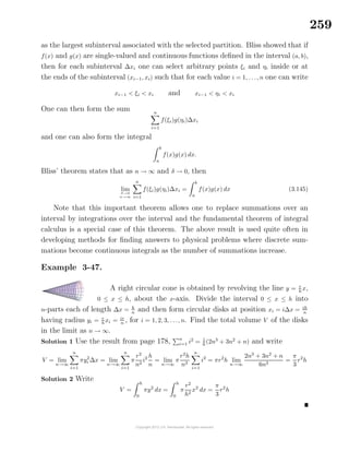
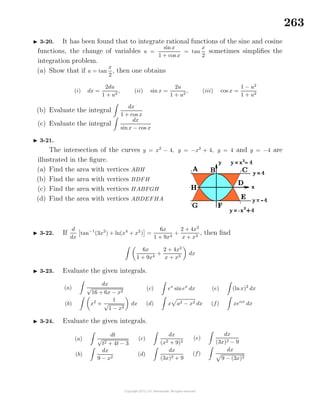
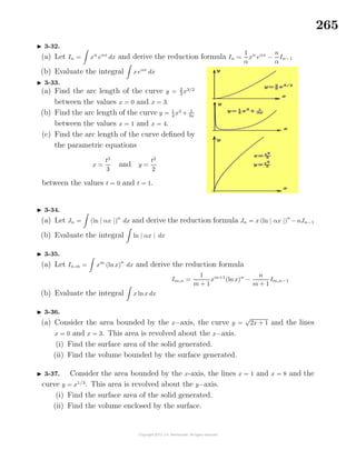
![266
3-38. The average value of a function y = y(x) over the interval [a, b] is given by
¯y =
1
b − a
b
a
y(x) dx and the weighted average of the function y = y(x) is given by
¯yw =
b
a
w(x)y(x) dx
b
a
w(x) dx
where w = w(x) is called the weight function.
(a) Find the average value of y = y(x) = sinx over the interval [0, π].
(b) Find the weighted average of y = y(x) = sin x over the interval [0, π] with respect
to the weight function w = w(x) = x.
(c) Find the weighted average of y = y(x) = sin x over the interval [0, π] with respect
to the weight function w = w(x) = cos2
x
(d) Where does the weight function place the most emphasis in calculating the
weighted average in parts (b) and (c)?
3-39. Find the area under the given curves from x0 to x1.
(a) y = x x2 + 1, x0 = 0, x1 = 2
(b) y =
x
√
x2 + 1
, x0 = 0, x1 = 2
(c) y = ln x, x0 = 1, x1 = e
(d) y = sin x, x0 = 0, x1 = π
(e) y = cos x, x0 = 0, x1 = π/2
(f) y = tan x, x0 = 0, x1 = π/4
3-40. Consider the triangular area bounded by the x−axis, the line y = x, 0 ≤ x ≤ 1
and the line y = 2 − x, 1 ≤ x ≤ 2. This area is revolved about the line x = 6 to form a
solid of revolution.
(i) Find the surface area of the solid generated.
(ii) Find the volume of the solid generated.
3-41. The line y = r = a constant, for 0 ≤ x ≤ h is rotated about the x−axis to form
a right circular cylinder of base radius r and height h.
(a) Use calculus and find the volume of the cylinder.
(b) Use calculus and find the lateral surface area of the cylinder.
3-42. Sketch the region of integration for the double integral
I =
1
0
4−x
x
f(x, y) dy dx.
3-43. The line y = r
h
x for 0 ≤ x ≤ h is rotated about the x−axis to form a right
circular cone of base r and height h.
(a) Use calculus and find the volume of the cone.
(b) Use calculus and find the lateral surface area of the cone.](https://image.slidesharecdn.com/calculusvolume-1-160216221448/85/Calculus-volume-1-274-320.jpg)
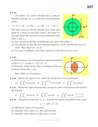
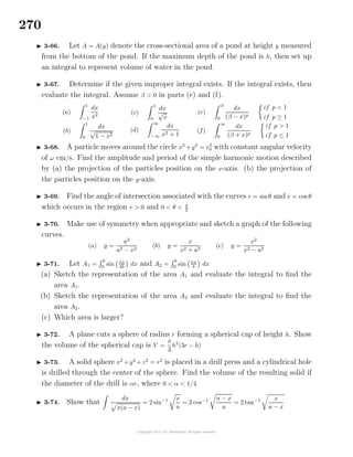
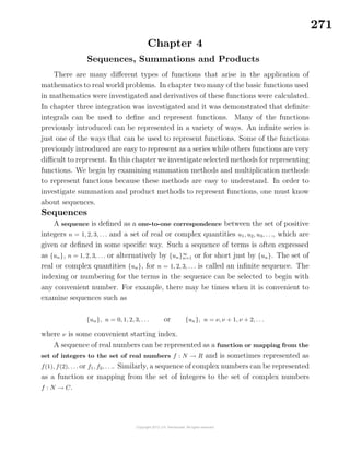
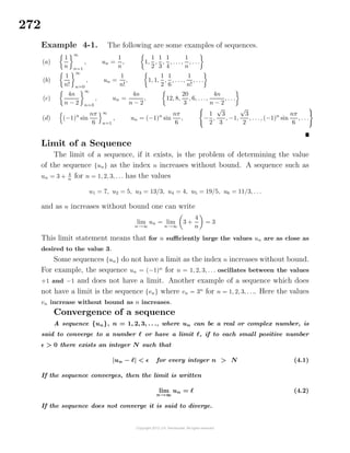
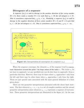
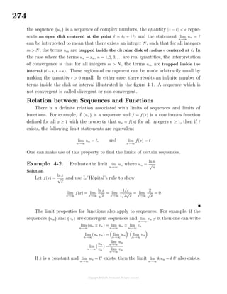
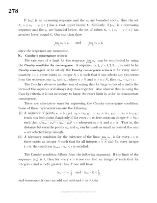
![283
Convergence and Divergence of a Series
The infinite series
∞
j=1
uj is said to converge to a limit U, or is said to have a
sum U, whenever the sequence of partial sums {Un}, has a finite limit, in which
case one can write lim
n→∞
Un = U. If the sequence of partial sums {Un} becomes
unbounded, is oscillatory or the limit lim
n→∞
Un does not exist, then the infinite
series is said to diverge.
Example 4-5. Divergent finite oscillatory and infinite oscillatory
Consider the series
∞
n=0
(−1)n
= 1 − 1 + 1 − 1 + 1 − 1 + · · · which has the partial sums
U1 = 1, U2 = 0, U3 = 1, U4 = 0, · · ·. These partial sums oscillate between the finite values
of 0 and 1 and so the sequence of partial sums is called a finite oscillatory sequence.
In this case the series is said to diverge.
In contrast consider the series
∞
n=0
(−1)n
2n
= 1−2+4−8+16−32+· · · which has the
partial sums U1 = 1, U2 = −1, U3 = 3, U4 = −5, U5 = 11, · · ·. Here the sequence of partial
sums become infinite oscillatory and so the series is said to diverge.
Example 4-6. Harmonic series
Consider the harmonic series H =
∞
m=1
1
m
which has the nth partial sum4
Hn = 1 +
1
2
+
1
3
+
1
4
+ · · · +
1
n
Nicole Oresme (1323-1382), a French mathematician and scholar who studied infinite
series, examined this series. His analysis considers the above finite sum, using the
value n = 2m
, where he demonstrated that the terms within the partial sum Hn can
be grouped together and expressed in the form
Hn = 1 +
1
2
+ (
1
3
+
1
4
) + (
1
5
+
1
6
+
1
7
+
1
8
) + · · · +
1
2m−1 + 1
+
1
2m−1 + 2
+ · · · +
1
2m
4
The nth partial sum of the harmonic series occurs in numerous areas of mathematics, statistics and probability
theory and no simple formula has been found to represent the sum Hn. The sums Hn are also known as harmonic
numbers, with H0 = 0. A complicated formula for Hn is given by Hn = γ + d
dz
Log [Γ(z)] where γ is the
Euler-Mascheroni constant and Γ(z) is the Gamma function.](https://image.slidesharecdn.com/calculusvolume-1-160216221448/85/Calculus-volume-1-291-320.jpg)
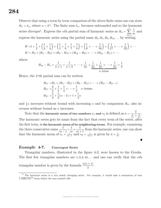
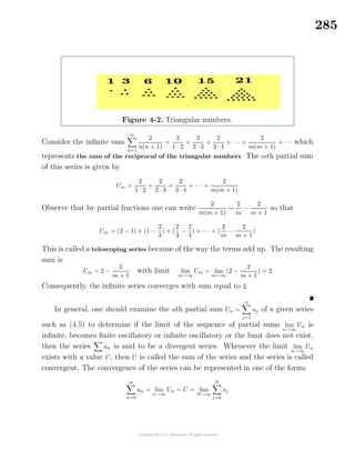
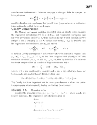
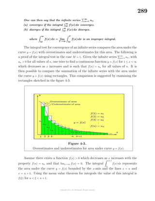
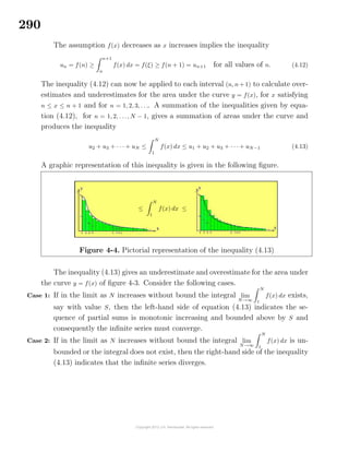
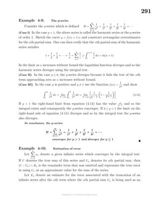
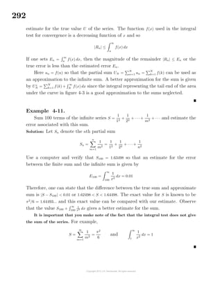
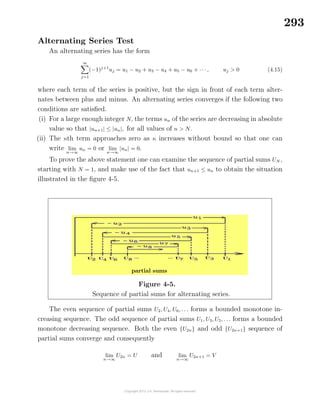
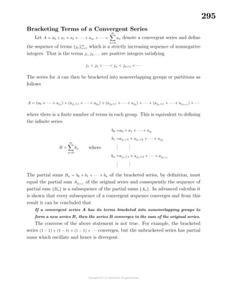
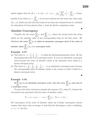
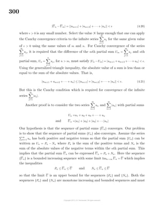
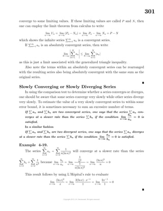
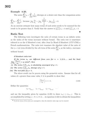
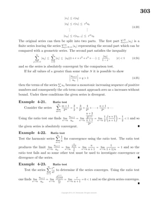
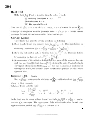
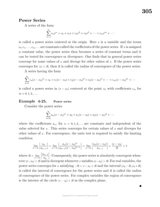
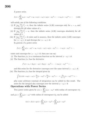
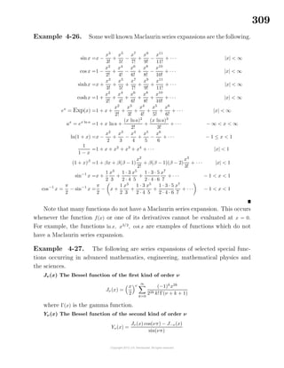
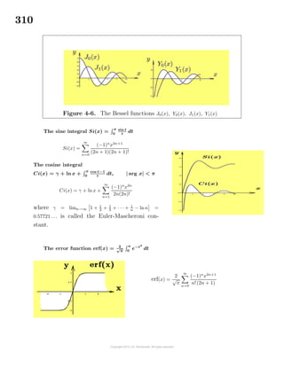

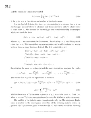
![320
Sch¨omilch and Roche Remainder Term
Still another form for the remainder term associated with the Taylor series ex-
pansion is obtained from the following arguments. Let f(x), f (x), . . ., f(n+1)
(x) all be
defined and continuous on the interval [x0, x0 + h] and construct the function
F(x) = f(x) +
n
m=1
(x0 + h − x)m
m!
f(m)
(x) + (x0 + h − x)p+1
A (4.63)
where A and p are nonzero constants. Select the constant A such that
F(x0 + h) =f(x0 + h)
and F(x0) =f(x0) +
n
m=1
hm
m!
f(m)
(x) + hp+1
A = f(x0 + h),
(4.64)
then F(x) satisfies all the conditions of Rolle’s theorem so there must exist a point
x = ξ = x0 + θh, 0 < θ < 1, such that F (ξ) = 0. Differentiate the equation (4.63) and
show
F (x) = f (x)+
n
m=1
(x0 + h − x)m
m!
f(m+1)
(x) −
m(x0 + h − x)m−1
m!
f(m)
(x) −(p+1)(x0+h−x)p
A
which can be simplified as follows.
F (x) =
n
m=1
(x0 + h − x)m
m!
f(m+1)
(x) −
n
m=2
m(x0 + h − x)m−1
m!
f(m)
(x) − (p + 1)(x0 + h − x)p
A
F (x) =
n
m=1
(x0 + h − x)m
m!
f(m+1)
(x) −
n−1
i=1
(x0 + h − x)i
i!
f(i+1)
(x) − (p + 1)(x0 + h − x)p
A
F (x) =
(x0 + h − x)n
n!
f(n+1)
(x) − (p + 1)(x0 + h − x)p
A
(4.65)
At x = ξ = x0 + θh it follows that
F (ξ) =
(h − θh)n
n!
f(n+1)
(ξ) − (p + 1)(h − θh)p
A = 0
a condition which requires that
A =
[h(1 − θ)]n−p
(p + 1) n!
f(n+1)
(ξ) (4.66)
Substituting A from equation (4.66) into the equation (4.64) produces the result
f(x0 + h) = f(x0) +
n
m=1
hm
m!
f(m)
(x0) +
hp+1
[h(1 − θ)]n−p
(p + 1) n!
f(n+1)
(ξ)](https://image.slidesharecdn.com/calculusvolume-1-160216221448/85/Calculus-volume-1-328-320.jpg)
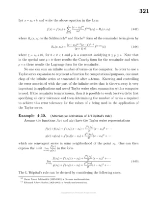
![322
Case 1 If f(x0) = 0 and g(x0) = 0 but g (x0) = 0, then equation (4.69) reduces to
lim
x→x0
f (x0) +
f (x0)
2!
(x − x0) +
f (x0)
3!
(x − x0)2
+ · · ·
g (x0) +
g (x0)
2!
(x − x0) +
g (x0)
3!
(x − x0)2
+ · · ·
=
f (x0)
g (x0)
= lim
x→x0
f (x)
g (x)
(4.70)
and so L´Hˆopital’s rule takes on the form
lim
x→x0
f(x)
g(x)
= lim
x→x0
f (x)
g (x)
Case 2 If f(x0) = 0, f (x0) = 0, g(x0) = 0 and g (x0) = 0, but g (x0) = 0, then equation (4.69)
reduces to the form
lim
x→x0
f (x0)
2!
+
f (x0)
3!
(x − x0) + · · ·
g (x0)
2!
+
g (x0)
3!
(x − x0) + · · ·
=
f (x0)
g (x0)
= lim
x→x0
f (x)
g (x)
(4.71)
and so in this case the L´Hˆopital’s rule takes on the form
lim
x→x0
f(x)
g(x)
= lim
x→x0
f (x)
g (x)
= lim
x→x0
f (x)
g (x)
The above examples illustrate that one can reapply L´Hˆopital’s rule whenever
the ratio of derivatives gives an indeterminate form.
Indeterminate forms 0 · ∞, ∞ − ∞, 00
, ∞0
, 1∞
If the limit lim
x→x0
f(x)
g(x)
=
0
0
or lim
x→x0
f(x)
g(x)
=
∞
∞
, then the limits are said to have
indeterminate forms and are calculated using the L´Hˆopital’s rule
lim
x→x0
f(x)
g(x)
= lim
x→x0
f (x)
g (x)
if the limit exists.
Other indeterminate forms are
lim
x→x0
f(x)g(x) = 0 · ∞ or lim
x→x0
f(x)g(x) = ∞ · 0
lim
x→x0
[f(x) − g(x)] = ∞ − ∞
lim
x→x0
f(x)g(x)
= 00
lim
x→x0
f(x)g(x)
= ∞0
lim
x→x0
f(x)g(x)
= 1∞
The general procedure used to investigate these other indeterminate forms is
to use some algebraic or trigonometric transformation that reduces these other in-
determinate forms to the basic forms 0
0
or ∞
∞
so that L´Hˆopital’s rule can then be
applied. The following examples illustrate some of these techniques.](https://image.slidesharecdn.com/calculusvolume-1-160216221448/85/Calculus-volume-1-330-320.jpg)
![323
Example 4-31. Evaluate the limit lim
x→0
[csc x · ln(1 + x)]
Solution If x = 0 is substituted into the functions given one obtains ∞ · 0 which is
an indeterminate form. Products of functions can be written in alternative forms
using algebra. For example,
f(x) · g(x) =
f(x)
1
g(x)
or f(x) · g(x) =
g(x)
1
f(x)
If the given limit is expressed in the form lim
x→0
ln(1 + x)
sin x
, then one can use L´Hˆopital’s
rule to investigate the limit. One finds
lim
x→0
ln(1 + x)
sin x
= lim
x→0
1
1 + x
cos x
= 1
Example 4-32. Evaluate the limit lim
x→π/2
(sec x − tanx)
Solution Investigating this limit one finds that it depends upon how x approaches
π/2. One finds lim
x→π/2
(sec x − tan x) = lim
x→π/2
sec x − lim
x→π/2
tan x = ±(∞ − ∞) which is an
indeterminate form. Using appropriate trigonometric identities the given limit can
be expressed in an alternative form where L´Hˆopital’s rule applies. One can write
lim
x→π/2
(sec x − tanx) = lim
x→π/2
1
cos x
−
sin x
cos x
= lim
x→π/2
1 − sinx
cos x
= lim
x→π/2
− cos x
− sinx
=
0
−1
= 0
Example 4-33. Evaluate the limit lim
x→0
|x|x
Solution This limit gives the indeterminate form 00
. One can use the identity
|x| = eln |x|
and write
lim
x→0
|x|x
= lim
x→0
ex·ln |x|
= elimx→0 x·ln |x|
Here limx→0 x · ln |x| gives the indeterminate form 0 · (−∞). Writing
lim
x→0
x · ln |x| = lim
x→0
ln |x|
1
x
one can apply L´Hˆopital’s rule and show
lim
x→0
x · ln|x| = lim
x→0
ln |x|
1
x
= lim
x→0
1
x
−1
x2
= lim
x→0
(−x) = 0
Consequently, one can write lim
x→0
|x|x
= lim
x→0
ex·ln |x|
= e0
= 1](https://image.slidesharecdn.com/calculusvolume-1-160216221448/85/Calculus-volume-1-331-320.jpg)
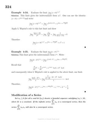
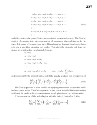
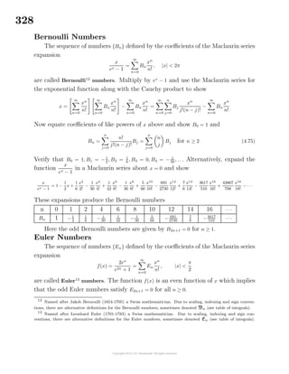
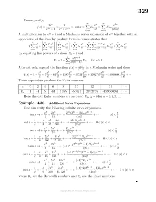
![330
Functions Defined by Series
If {fn(x)} , n = 0, 1, 2, . . ., denotes an infinite sequence of functions defined over an
interval [a, b], then other functions can be constructed from these functions.
Many functions F(x) are defined by an infinite series having the form
F(x) =
∞
j=0
cjfj(x) (4.76)
where c0, c1, c2, . . . are constants. To study the convergence or divergence of such
series one should consider the sequence of finite sums {Fn(x)} where
Fn(x) =
n
j=0
cjfj(x) = c0f0(x) + c1f1(x) + · · · + cnfn(x) (4.77)
for n = 0, 1, 2, . . .. The sequence {Fn(x)} is called the sequence of partial sums asso-
ciated with the infinite series (4.76). The infinite series is said to converge if the
sequence of partial sums converges. If the sequence of partial sums diverges, then
the infinite series (4.76) is said to diverge.
The sequence is said to converge uniformly on an interval a ≤ x ≤ b to a function
F(x), if for every > 0 there exists an integer N such that
|Fn(x) − F(x)| < , for all n > N and for all x ∈ [a, b] (4.78)
Example 4-37.
(a) From the sequence of functions {sin nx} one can define the Fourier sine series
expansions
F(x) =
∞
n=1
bn sin nx (4.79)
where the bn coefficients are constants.
(b) From the sequence of functions {cos nx} one can define the Fourier cosine series
expansions
G(x) = a0 +
∞
n=1
an cos nx (4.80)
where the an coefficients are constants. The study of Fourier series expansions
has many applications in advanced mathematics courses.](https://image.slidesharecdn.com/calculusvolume-1-160216221448/85/Calculus-volume-1-338-320.jpg)
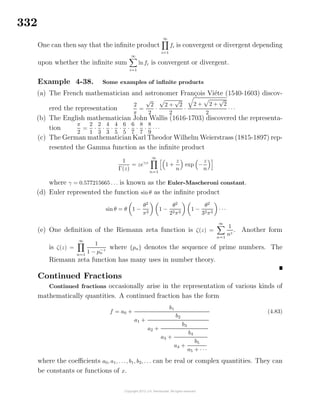
![333
In general, when using the continued fraction representation14
given by equation
(4.83) the coefficients a0, {ai} and {bi}, i = 1, 2, 3, . . . can be constants or functions of
x and these coefficients can be finite in number or infinite in number. The pattern
of numerator over denominator can go on forever or the ratios can terminate after
a finite number of terms. A finite continued fraction has the form
fn = a0 +
b1
a1 +
b2
a2 +
b3
a3 +
b4
a4 + · · · +
bn
an
(4.84)
which terminates with the ratio
bn
an
.
Terminology
(i) The numbers b1, b2, b3, . . . are called the partial numerators.
(ii) The numbers a1, a2, a3, . . . are called the partial denominators.
(iii) If the partial numerators bi, for i = 1, 2, 3, . . . are all equal to 1 and all the ai
coefficients have integer values, then the continued fraction is called a simple or
regular continued fraction. A simple continued fraction is sometimes represented
using the shorthand list notation f = [a0 ; a1, a2, a3, . . .] where the ai, i = 0, 1, 2, . . .
are called the quotients of the regular continued fraction.
(iv) The continued fraction is called generalized if the terms ai and bi for i = 1, 2, 3, . . .
do not have any restrictions as to their form.
(v) The ratio of terms notation as illustrated by the equations (4.83) and (4.84) is
awkward and takes up too much space in typesetting and is often abbreviated
to the shorthand Pringsheim15
notation
fn = a0 +
|
b1
a1
|
+
|
b2
a2
|
+ · · · +
|
bn
an
|
(4.85)
for a finite continued fraction terminating with the bn
an
term and in the form
f = a0 +
|
b1
a1
|
+
|
b2
a2
|
+ · · · +
|
bn
an
|
+ · · · (4.86)
14
Take note that the starting index is zero. Some notations use a different starting index which can lead to
confusion at times.
15
Alfred Israel Pringsheim (1850-1941) a German mathematician.](https://image.slidesharecdn.com/calculusvolume-1-160216221448/85/Calculus-volume-1-341-320.jpg)
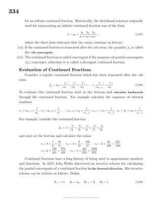
![336
Convergent Continued Fraction
Examine the sequence of partial convergents fn =
An
Bn
associated with a given
continued fraction. If the limit lim
n→∞
fn = lim
n→∞
An
Bn
= f exists, then the continued
fraction is called convergent. Otherwise, it is called a divergent continued fraction.
Regular Continued Fractions
Regular continued fractions of the form
f = a0 +
|
1
a1
|
+
|
1
a2
|
+ · · · +
|
1
an
|
+ · · · (4.93)
are the easiest to work with and are sometimes represented using the list notation
f = [a0 ; a1, a2, a3, . . ., an, . . .] (4.94)
Example 4-39. (Continued fraction)
The representation of a number x as a regular continued fraction of the form
of equation (4.93) is accomplished using the following algorithm to calculate the
partial denominators ai for i = 1, 2, 3, . . ., n.
a0 =[x], x1 =
1
x − a0
a1 =[x1], x2 =
1
x1 − a1
...
...
an =[xn], xn+1 =
1
xn − an
(4.95)
where [x] is the greatest integer in x function. For example, to represent the number
x = π = 3.1415926535897932385 . . . as a continued fraction one finds
a0 =[x] = 3, x1 =
1
π − 3
= 7.0625133059310457698 . . .
a1 =[x1] = 7, x2 =
1
x1 − 7
= 15.9965944066857199 . . .
a2 =[x2] = 15, x3 =
1
x2 − a2
= 1.0034172310133726 . . .
a3 =[x3] = 1, x4 =
1
x3 − a3
= 292.63459101440 . . .
and so one representation of π as a continued fraction has the list form given by
f = π = [3 ; 7, 15, 1, 292, . . .] which gives the following rational number approximations
for π.
f1 = 3, f2 =
22
7
, f3 =
333
106
, f4 =
355
113
, f5 =
103993
33102
, · · ·](https://image.slidesharecdn.com/calculusvolume-1-160216221448/85/Calculus-volume-1-344-320.jpg)
![337
Continue the above algorithm and show
f = π = [3 ; 7, 15, 1, 292, 1, 1, 1, 2, 1, 3, 1, 14, . . .]
A generalized continued fraction expansion for π can be obtained from the arctanx
function evaluated at x = 1 to obtain the representation
π
4
=
|
1
1
|
+
|
1
3
|
+
|
4
5
|
+
|
9
7
|
+
|
16
9
|
+
|
25
11
|
+
|
36
13
|
+ · · ·
where all the partial numerators after the first term are squares and the partial
denominators are all odd numbers.
Other examples of mathematical constants represented by regular continued
fractions are
e =[2 ; 1, 2, 1, 1, 4, 1, 1, 6, 1, 1, 8, 1, 1, 10, 1, 1, 12, 1, . . .]
γ =[0 ; 1, 1, 2, 1, 2, 1, , 4, 3, 13, 5, 1, 1, 8, 1, 2, 4, 40, 1, . . .]
Euler’s Theorem for Continued Fractions
Euler showed that the infinite series U = u1 + u2 + u3 + · · · can be represented by
the continued fraction
U =
|
u1
1
|
−
|
u2
u1 + u2
|
−
|
u1u3
u2 + u3
|
−
|
u2u4
u3 + u4
|
−
|
u3u5
u4 + u5
|
− · · · −
|
unun+2
un+1 + un+2
|
− · · · (4.96)
The convergence or divergence of this continued fraction is then closely related to
the convergence or divergence of the infinite series which it represents.
Gauss Representation for the Hypergeometric Function
Carl Fredrich Gauss (1777-1855) a famous German mathematician showed that
the hypergeometric function could be represented by the continued fraction
2F1(a + 1, b ; c + 1 ; z)
2F1(a, b ; c ; z)
=
|
1
1
|
+
|
(a−c)b
c(c+1)
z
1
|
+
|
(b−c−1)(a+1)
(c+1)(c+2)
z
1
|
+
|
(a−c−1)(b+1)
(c+2)(c+3)
z
1
|
+
|
(b−c−2)(a+2)
(c+3)(c+4)
z
1
|
+ · · ·
Representation of Functions
There are many areas of mathematics where functions f(x) are represented in
the form of an infinite generalized continued fraction having the form
f(x) = a0(x) +
b1(x)
a1(x) +
b2(x)
a2(x) +
b3(x)
a3(x) + · · · +
bn(x)
an(x) + rn+1(x)
(4.97)](https://image.slidesharecdn.com/calculusvolume-1-160216221448/85/Calculus-volume-1-345-320.jpg)
![339
r2 =
4x2
a3 + r3
=⇒ r3 =
4x2
r2
− 5 =
9
7
x2
−
16
49
x4
+ · · ·
r3 =
9x2
a4 + r4
=⇒ r4 =
9x2
r3
− 7 =
16
9
x2
−
400
891
x4
+ · · ·
...
...
rn =
(nx)2
an+1 + rn+1
=⇒ rn+1 =
(nx)2
rn
− [2(n + 1) − 1] =
(n + 1)2
2(n + 1) + 1
x2
+ · · ·
Observe that lim
x→0
ri(x) = 0 so it is possible to calculate the coefficients ai, i = 1, 2, 3, . . .
and show
(a1, a2, a3, a4, a5, . . ., an, . . .) = (1, 3, 5, 7, 9, . . ., 2n + 1, . . .)
Evaluating the arctangent function at x = 1 gives the continued fraction
π
4
=
|
1
1
|
+
|
1
3
|
+
|
4
5
|
+
|
9
7
|
+
|
16
9
|
+
|
25
11
|
+
|
36
13
|
+ · · ·
given in the previous example 4-29.
Fourier Series
Consider two functions f = f(x) and g = g(x) which are continuous over the
interval a ≤ x ≤ b. The inner product of f and g with respect to a weight function
r = r(x) > 0 is written (f, g) or (g, f) and is defined
(f, g) = (g, f) =
b
a
r(x)f(x)g(x) dx (4.101)
The inner product of a function f with itself is called a norm squared and written
f 2
. The norm squared is defined
f 2
= (f, f) =
b
a
r(x)f2
(x) dx (4.102)
with norm given by f = (f, f). If the inner product of two functions f and g
with respect to a weight function r is zero, then the functions f and g are said to be
orthogonal functions.](https://image.slidesharecdn.com/calculusvolume-1-160216221448/85/Calculus-volume-1-347-320.jpg)
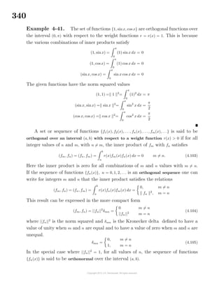
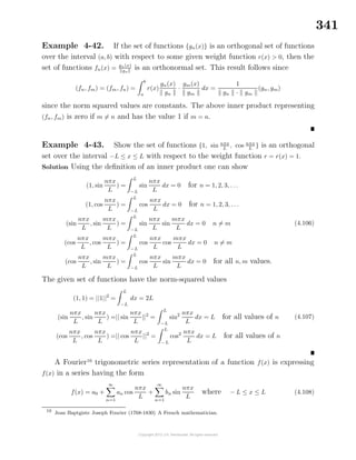
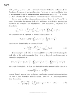
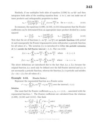

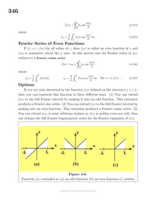
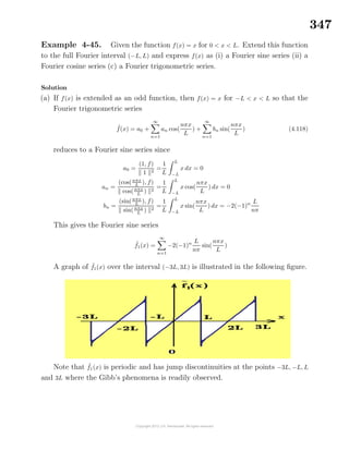
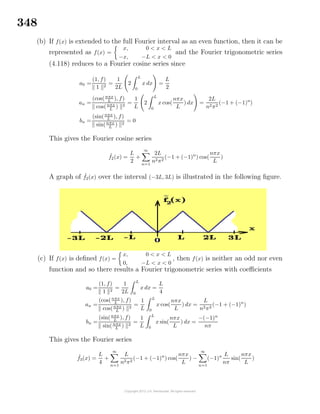
![353
4-17. Newton’s root finding method To deter-
mine where a given curve y = f(x) crosses the
x-axis one can select an initial guess x0 and if
f(x0) = 0 one can then calculate f (x0). From
the values f(x0) and f (x0) one can construct the
tangent line to the curve y = f(x) at the point
(x0, f(x0)). This tangent line given by y − f(x0) = f (x0)(x − x0).
(a) Show the tangent line intersects the x-axis at the point x1 = x0 − f(x0)/f (x0)
(b) Form the sequence {xn} where xn = xn−1 − f(xn−1)/f (xn−1) for n = 1, 2, 3, . . .
(c) Give a geometric interpretation to what this sequence is doing. Hint: What has
been done once can be done again.
(d) If y = f(x) = x2
− 3x + 1 and x0 = 1, find using a calculator x1, x2, x3 and x4
(e) If y = f(x) = x2
− 3x + 1 and x0 = 2, find using a calculator x1, x2, x3 and x4
(f) Sketch the curve y = f(x) = x2
− 3x + 1 and find the roots of the equation f(x) = 0.
(g) What happens if the initial guess x0 is bad? Say x0 = 3/2 for the above example.
4-18. Let fn(x) =
xn
n(n + 1)
(a) Show that
∞
n=1
fn(9/10) converges. (b) Show that
∞
n=1
fn(10/9) diverges.
4-19. Given the infinite series
∞
n=2
1
n [lnn]p
, with p > 0.
(a) Show the series converges for p > 1.
(b) Show the series diverges for p ≤ 1.
Hint: Let f0(t) = t, f1(t) = lnf0(t), f2(t) = ln f1(t), . . ., fn+1(t) = ln fn(t) and show
dt
f0(t)f1(t)f2(t) · · ·fm−1(t) [fm(t)]
p =
fm+1(t), p = 1
−1
(p−1)
[fm(t)]
p−1
, p = 1
and then examine
∞
n=2
1
n [lnn]p
=
∞
n=2
1
f0(n)[f1(n)]p
4-20. Show that if the series
∞
n=1
un converges, then the series
∞
n=1
1
un
diverges.
4-21. If Un = 1
3
n3
= 1
3
n(n + 1)(n + 2), show ∆Uk = Uk+1 − Uk = (k + 1)(k + 2) and find
the sum of the series Sn = 1 · 2 + 2 · 3 + 3 · 4 + · · · + n · (n + 1) =
n−1
k=0
(k + 1)(k + 2) =
n−1
k−0
∆Uk](https://image.slidesharecdn.com/calculusvolume-1-160216221448/85/Calculus-volume-1-361-320.jpg)
![354
4-22. Reversion of series
(a) Given the series
y = y(x) = 1 − (x − 1) +
(x − 1)2
2!
−
(x − 1)3
3!
+ · · · 22(a)
and it is required that you solve for x − 1 in terms of y to obtain a series of the
form
(x − 1) = A1(y − 1) + A2(y − 1)2
+ A3(y − 1)3
+ A4(y − 1)4
+ · · · 22(b)
where A1, A2, A3, A4 . . . are constants to be determined. Substitute equation 22(b)
into equation 22(a) and expand all terms. Equate like powers of (y − 1) and
obtain a system of equations from which the constants A1, A2, A3, A4, . . . can be
determined.
(b) If the original series in part(a) is y = e−(x−1)
and the series obtained by reversion
is the function (x − 1) = − lny, expanded in a series about y = 1, then examine
the approximation for x − 1 by truncation of your series after the A4 term. Let
E = E(y) denote the error in using this truncated series to solve for x − 1. Plot a
graph of the error E = E(y) for 1 ≤ y < 2.
4-23. Examine the given alternating series to determine if they converge.
(a)
∞
n=1
1
(−3)n−1
(b)
∞
n=2
(−1)n 1
lnn
(c)
∞
n=1
(−1)n−1
n!
(d)
∞
n=1
(−1)n
√
n
(e)
∞
n=1
(−1)n+1
n
(f)
∞
n=1
(−1)n+1
n
n2 + 1
4-24. Use the root test to determine if the given series converge.
(a)
∞
n=2
1
[ln n]n
(b)
∞
n=1
nn
24n
(c)
∞
n=1
n2
2n
(d)
∞
n=1
n
n2 + 1
n
(e)
∞
n=1
1
nn
(f)
∞
n=1
1
n + 1
n
4-25. Test the following series to determine convergence or divergence.
(a)
∞
n=1
(−1)n
n!
(b)
∞
n=1
n10
(1.001)n
(c)
∞
n=1
sinn
(π/3)
(d)
∞
n=1
n
2n
(e)
∞
n=1
n3
3n
(f)
∞
n=1
3n
n!](https://image.slidesharecdn.com/calculusvolume-1-160216221448/85/Calculus-volume-1-362-320.jpg)
![357
4-36. The continued fraction function
yn = yn(x) =
Pn(x)
Qn(x)
= α0 +
|
1
α1
|
+
|
1
α2
|
+ · · · +
|
1
αn
|
+
|
1
x
|
where α0, α1, α2, . . ., αn are constants, represents a rational function of x.
(a) Show that
dy1
dx
=
1
[Q1(x)]2
(b) Show that
dy2
dx
=
−1
[Q2(x)]2
(c) Show that
dy3
dx
=
1
[Q3(x)]2
(d) Can you show that in general
dyn
dx
= (−1)n 1
[Qn(x)]2
4-37. Euler used the product formula sin θ = θ 1 −
θ
π
2
1 −
θ
2π
2
· · · 1 −
θ
nπ
2
· · ·
to represent sine of θ. Differentiate this relation and show θ cot θ = 1+2θ2
∞
n=1
1
θ2 − n2π2
4-38. Assume that un and vn are two infinite series of positive terms and that
there exists an integer N such that for all n > N the inequality un ≤ Kvn for some
positive constant K.
(i) If the series vn converges, prove the series un converges.
(ii) If the series un diverges, prove the series vn diverges.
4-39. Show that the alternating p-series
∞
n=1
(1)n+1 1
np
converges if p > 0.
4-40. Consider the geometric series
1
1 − z
= 1 + z + z2
+ z3
+ · · · + zn
+ · · · where
z = reiθ
, |z| < 1 and i2
= −1. Show that by equating real and imaginary parts
1 − r cos θ
1 − 2r cos θ + r2
=1 + r cos θ + r2
cos 2θ + · · · + rn
cos nθ + · · ·
r sin θ
1 − 2r cos θ + r2
=r sin θ + r2
sin 2θ + · · · + rn
sinnθ + · · ·
Hint: Use Euler identity eiθ
= cos θ + i sin θ
4-41.
(a) Show {sin nx}, n = 1, 2, 3, . . . is an orthogonal sequence over the interval (0, π) with
respect to the weight function r = 1.
(b) Scale the above sequence to construct an orthonormal sequence over the given
interval.](https://image.slidesharecdn.com/calculusvolume-1-160216221448/85/Calculus-volume-1-365-320.jpg)

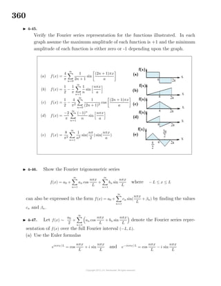
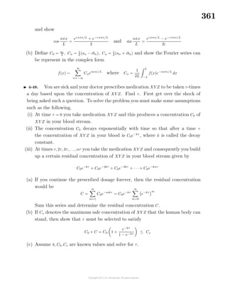
![363
Chapter 5
Applications of Calculus
Selected problems from various areas of physics, chemistry, engineering and the
sciences are presented to illustrate applications of the differential and integral calcu-
lus. Many of these selected topics require knowledge of basic background material,
such as terminology and fundamentals, associated with the area of application. Con-
sequently, much of this chapter gives a presentation of selected basic material from
areas of engineering, physics, chemistry and the sciences which is required knowledge
for the understanding of many scientific applications of the differential and integral
calculus.
Related Rates
The rate of change of a quantity Q = Q(t) with respect to time t is denoted by the
derivative
dQ
dt
. Problems which involve rates of change of two or more time dependent
variables are referred to as “related rate problems”. The general procedure for
solving related rate problems is something like the following.
1. If necessary, define the variables of the problem and make note of the units of
measurement being used. For example, one could write [Q] = cubic centimeters
which is read1
“The dimension of Q is cubic centimeters”.
2. Find how the variables of the problem are related for all values of time t being
considered.
3. Determine if the variables of the problem, or their derivatives, have known values
at some particular instant of time.
4. Find the rate of change relation between the variables by differentiating the
relation or relations found in step 2 above.
5. Evaluate the results in step 4 at the particular instant of time specified.
Example 5-1. Consider a large inverted right circular cone with altitude H
and base radius R where water runs into the cone at the rate of 3 cubic feet per
second. How fast is the water level rising when the water level, as measured from
the vertex of the cone, is 4 feet? Here the base radius R and height H of the cone
are considered as fixed constants.
1
Notation introduced by J.B.J. Fourier, theorie analytique de la chaleur, Paris 1822.](https://image.slidesharecdn.com/calculusvolume-1-160216221448/85/Calculus-volume-1-371-320.jpg)
![364
Solution Let r = r(t), [r] = feet, denote the radius of the water level at time t and let
h = h(t), [h] = feet, denote the height of the water level at time t, [t] = minutes. One
can then express the volume V of water in the cone at time t as
V = V (t) =
π
3
r2
h, [V ] = cubic feet (5.1)
Using similar triangles one finds that there is
a relation between the variables r and h given by
r
h
=
R
H
or r =
R
H
h (5.2)
The given problem states that
dV
dt
= 3, where
[
dV
dt
] = ft3
/min and it is required to find
dh
dt
, when
h = 4 feet. Differentiating equation (5.1) with
respect to time t gives
dV
dt
=
π
3
r2 dh
dt
+ 2r
dr
dt
h (5.3)
and differentiating equation (5.2) with respect to t gives
dr
dt
=
R
H
dh
dt
(5.4)
since R and H are constants. Substituting the results from the equations (5.2) and
(5.4) into the equation (5.3) gives
dV
dt
=
π
3
R2
H2
h2 dh
dt
+ 2
R
H
h
R
H
dh
dt
h
which simplifies to
dV
dt
= π
R2
H2
h2 dh
dt
(5.5)
Now one can evaluate the equation (5.5) when h = 4 to obtain
3 = π
R2
H2
(4)2 dh
dt
or
dh
dt
=
3
16π
H2
R2
,
dh
dt
= ft/min (5.6)
Alternatively, one could have substituted the equation (5.2) into the equation (5.1)
to obtain
V =
π
3
R2
H2
h3
(5.7)
and then differentiate the equation (5.7) with respect to time t to obtain
dV
dt
=
π
3
R2
H2
3h2 dh
dt
and evaluating this last equation when h = 4 gives the same result as equation (5.6).](https://image.slidesharecdn.com/calculusvolume-1-160216221448/85/Calculus-volume-1-372-320.jpg)
![365
Example 5-2. Two roads intersect at point 0 at an angle of 60 degrees. Assume
car A moves away from 0 on one road at a speed of 50 miles per hour and a second
car B moves away from point 0 at 60 miles per hour on the other road. Let a denote
the distance from point 0 for car A and let b denote the distance from point 0 for
car B. How fast is the distance between the cars changing when a = 1 mile and b = 2
miles.
Solution
Let r denote the distance between the cars A and B
and use the law of cosines to show
r2
= a2
+ b2
− 2ab cos θ
Differentiate this relation with respect to time t and show
2r
dr
dt
= 2a
da
dt
+ 2b
db
dt
− 2 a
db
dt
+
da
dt
b cos θ, θ is a constant
and then solve for the rate of change
dr
dt
to obtain
dr
dt
=
a
da
dt
+ b
db
dt
− a
db
dt
+
da
dt
b cos θ
√
a2 + b2 − 2ab cos θ
Substitute into this equation the values
a =1 mi
da
dt
=50 mi/hr
b =2 mi
db
dt
=60 mi/hr
θ =
π
3
and show
dr
dt
= 30
√
3 miles per hour.
Example 5-3. Boyle’s2
law resulted from a study of an ideal compressed gas
at a constant temperature. Boyle discovered the relation PV = C = constant, where P
represents pressure, [P] = Pascal, abbreviated Pa, and V represents volume, [V ] = cm3
and C is a constant. If at some instant the pressure is P0 and the volume of the gas
has the value V0 and the pressure is increasing at the rate r0, [r0] = Pa/min, then at
what rate is the volume decreasing at this instant?
2
Robert Boyle (1627-1691) an Irish born chemist/mathematician.](https://image.slidesharecdn.com/calculusvolume-1-160216221448/85/Calculus-volume-1-373-320.jpg)
![366
Solution Here Boyle’s law is P V = P0V0 = constant, where the pressure and volume
are changing with respect to time. Differentiating this relation with respect to time
t gives the relation
P
dV
dt
+
dP
dt
V =
d
dt
(P0V0) = 0 (5.8)
Evaluating the equation (5.8) at the instant where
dP
dt
= r0, P = P0 and V = V0, one
finds
P0
dV
dt
+ r0V0 = 0 or
dV
dt
= −r0
V0
P0
The minus sign indicates that the volume is decreasing and the volume rate of change
has dimension, [
dV
dt
] = cm3
/min.
Note that Boyle’s law is a special case of the more general gas law given by
PV
T
= C = Constant relating pressure P, volume V and temperature T all having
appropriate units of measurements.
Newton’s Laws
Isaac Newton used his new mathematical knowledge of calculus to formulate
basic principles of physics in studying the motion of objects and particles. The
following are known as Newton’s laws of motion.
(i) Newton’s First Law
A body at rest tends to stay at rest or a body in a uniform straight line
motion tends to stay in motion unless acted upon by an external force.
(ii) Newton’s Second Law
The time rate of change of momentum3
of a body is proportional to the
resultant force that acts upon it.
(iii) Newton’s Third Law
For every action there is an equal and opposite reaction.
In the following discussions the symbols F, x, v, a, m, p, t are used to denote force,
distance, velocity, acceleration, mass, momentum and time. Time t is measured
in units of seconds, abbreviated (s). The symbol F is to denote force, measured
in units of Newton’s abbreviated4
(N). The quantity x denotes distance, measured
in meters, abbreviated (m). The velocity is denoted v =
dx
dt
and represents the
3
Momentum is defined as mass times velocity.
4
If a unit of measurement is named after a person, then the unit is capitalized, otherwise it is lower case.](https://image.slidesharecdn.com/calculusvolume-1-160216221448/85/Calculus-volume-1-374-320.jpg)
![369
since h is much less than the radius of the Earth re. The equation (5.14) can be used
to define the following terms.
The acceleration of gravity g is defined
g =
Gme
r2
e
(5.15)
and the weight W of an object of mass m due to gravity is defined
W = Fg = mg (5.16)
That is, the weight of an object is the force (force of gravity), by which an
object of mass m is pulled vertically downward toward the center of the Earth.
The dimensions of g and W are given by [g] = m/s2
, and [W] = kg·m/s2
= N. The
acceleration of gravity varies slightly over the surface of the Earth because the
radius of the Earth is not constant everywhere. If re is assumed to be constant,
then the acceleration of gravity is found to have the following values in the MKS,
FPS and CGS system of units
g = 9.807 m/s2
, g = 32.17 ft/s2
, g = 980.7 cm/s2
(5.17)
Example 5-4. Approximating Value of Escape Velocity
A rocket launched straight upward from the surface of the Earth will fall back
down if it doesn’t achieve the correct velocity. Let r = r(t) denote the distance of
the rocket measured from the center of the Earth and let m = m(t) denote the mass
of the rocket which changes with time. The forces acting on the rocket as it moves
upward are the thrust from the engines, the pull of gravity and resistance due to air
friction called a drag force. By Newton’s second law one can write
d
dt
(mv) =
d
dt
m
dr
dt
= Ftotal = Fthrust − Fgravity − Fdrag (5.18)
where v = v(t) =
dr
dt
is the velocity of the rocket. This is an equation, called a
differential equation, which describes the motion of the rocket. When you learn
more about aerodynamics you will learn how to represent the thrust force and drag
forces on the rocket and then you can solve the resulting differential equation.
Instead, let us solve a much simpler problem created by making assumptions
which will reduce the equation (5.18) to a form which is tractable7
7
When confronted with a very difficult problem to solve, one can always make assumptions to simplify the
problem to a form which can be solved. Many times an analysis of the simplified solution produces an incite into
how to go about solving the more difficult original problem.](https://image.slidesharecdn.com/calculusvolume-1-160216221448/85/Calculus-volume-1-377-320.jpg)
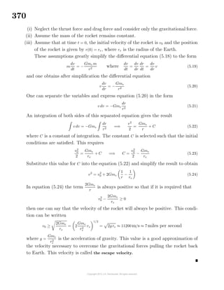
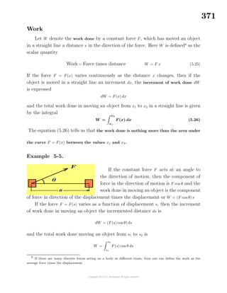
![372
Recall that force is measured in units called Newtons, where 1 N = 1 kg · m/s2
. Dis-
placement is measured in meters (m) so that work is force times distance and is
measured in units of Newton-meters or (N · m) and one can write [W] = N · m, which
is read, “The dimension of work is Newton-meter”. By definition 1 N · m = 1 Joule,
where Joule is abbreviated (J).
Energy
In the language of science the term energy is a scalar measure of a physical
systems ability to do work. There are many different kinds of energy. A few selected
types of energy you might have heard of are chemical energy, kinetic energy, various
kinds of potential energy, internal energy, elastic energy due to stretching or twisting,
heat energy, light energy and nuclear energy.
Kinetic Energy Ek
The energy associated with a body in motion is called kinetic energy and is
denoted by Ek. The kinetic energy is defined Ek =
1
2
mv2
, where m is the mass of
the body, [m] = kg and v is the velocity of the body, [v] = m/s. Kinetic energy is a
positive scalar quantity measured in the same units as work. One can verify that
[Ek] = kg · m2
/s2
= kg · m/s2
· m = N · m = J
Example 5-6. The work done by a constant force F moving an object in a
straight line through a distance s during a time t is given by the integral
W =
s
0
F ds (5.27)
Let s denote distance traveled during a time t with
ds
dt
= v denoting the velocity
and a =
dv
dt
=
d2
s
dt2
denoting the acceleration. Using Newton’s second law of motion
one can write
F = ma = m
dv
dt
= m
d2
s
dt2
, where
ds
dt
= v and
d2
s
dt2
=
dv
dt
= a (5.28)
Substituting the equation (5.28) into the equation (5.27) gives
W =
s
0
m
dv
dt
ds =
s
0
m
d2
s
dt2
ds =
t
0
m
d2
s
dt2
ds
dt
dt (5.29)
Observe the equation (5.29) is written as an integration with respect to time by
using the relations v =
ds
dt
and
dv
dt
=
d2
s
dt2
. If the object has an initial velocity v0 at
time t = 0, then the integration (5.29) can be expressed in the form
W =
t
0
m
dv
dt
v dt = m
t
0
d
1
2
v2
=
1
2
mv2
t
0
=
1
2
mv2
−
1
2
mv2
0 (5.30)](https://image.slidesharecdn.com/calculusvolume-1-160216221448/85/Calculus-volume-1-380-320.jpg)
![373
The equation (5.30) is a representation of the work-energy relation
“The work done by forces acting on a body
equals the change in kinetic energy of the body”
Potential Energy Ep
The energy associated with a body as a result of its position with respect to
some reference line is called the potential energy and is defined Ep = mg h, where m
is the mass of the body, [m] = kg, g is the acceleration of gravity, [g] = m/s2
and h
is the height of the body above the reference line, [h] = m. The potential energy is
sometimes called the gravitational potential energy. The potential energy is measured
in units of kg· m/s2
· m = N· m = J and has the same units of measurement as work.
The work done against gravity in lifting a weight from a height h1 to a height h2 is
given by
W =
h2
h1
−Fg dx =
h2
h1
−mg dx = −mg x
h2
h1
= −(mg h2 − mg h1) = −∆Ep
where −Fg = −W is the weight acting downward. One can say the work done equals
the change in potential energy.
Example 5-7. Consider a ball of mass m which is thrown vertically
upward with an initial velocity v0. Neglect air resistance
so that the only force acting on the ball is the force due
to gravity and construct a coordinate system with the
origin placed at the point where the ball is released.
Here the upward direction is taken as positive and by
Newton’s second law one can write
m
dv
dt
= −mg (5.31)
since the weight of the ball is mg and this force is acting downward. Separate the
variables in equation (5.31) and then integrate to obtain
v
v0
m dv = −mg
t
0
dt or mv − mv0 = −mgt (5.32)](https://image.slidesharecdn.com/calculusvolume-1-160216221448/85/Calculus-volume-1-381-320.jpg)
![374
If y denotes the distance of the ball above the reference axis, then the velocity of
the ball is given by v =
dy
dt
. The equation (5.32) can now be expressed in the form
m
dy
dt
= mv0 − mgt (5.33)
since the velocity v =
dy
dt
represents the change in the height of the ball as a function
of time. Multiply equation (5.33) by dt and integrate to obtain
m
y
0
dy =
t
0
[mv0 − mgt] dt or my = mv0t −
1
2
mgt2
(5.34)
Solve equation (5.32) for the variable t and substitute for t in equation (5.34) and
then simplify to show
1
2
mv2
+ mgy =
1
2
mv2
0 (5.35)
which can be interpreted as stating that the sum of the kinetic energy plus the
potential energy of the ball always has a constant value. Note that when the ball
reaches its maximum height, where y = h, the velocity of the ball is zero, and at this
time the equation (5.35) shows that the initial kinetic energy of the ball equals the
potential energy of the ball at its maximum height.
There are many more types of energy and all these energy types obey the law
of conservation of energy which states that there is no change in the total energy in
the Universe. Another way of saying this is to state that energy can be transformed,
but it cannot be created or destroyed.
First Moments and Center of Gravity
Consider a force F acting perpendicular to a
plane containing a line 0 − 0. The first moment
of a force F, also called a torque, is defined
Moment =(Force)(Lever arm distance)
M =F
(5.36)
where the lever arm is understood to represent
the shortest perpendicular distance from the line
0 − 0 to the line of action of the force F. The moment is a measure of the ability of
the force to produce a rotation about the line 0 − 0. In general a quantity times a
distance to a point, or times a distance to a line, or times a distance to a plane, is
called a moment of that quantity with respect to a point, line or plane.](https://image.slidesharecdn.com/calculusvolume-1-160216221448/85/Calculus-volume-1-382-320.jpg)
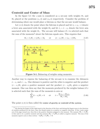
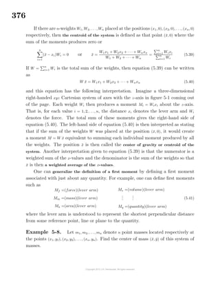
![377
Solution
Use the x and y-axes as the lines about which
one can take first moments associated with the
given point masses. If m =
n
i=1 mi is the total
sum of all the point masses, then if this mass
were placed at the point (¯x, ¯y) it would produce
first moments about these axes given by
Mx = m ¯y and My = m ¯x
These moments must be equivalent to the sum of the first moments produced by
each individual mass so that one can write
My = m ¯x =
n
i=1
mixi and Mx = m ¯y =
n
i=1
miyi
The center of mass of the system then has the coordinates (¯x, ¯y) where
¯x =
n
i=1 mixi
n
i=1 mi
=
My
m
and ¯y =
n
i=1 miyi
n
i=1 mi
=
Mx
m
Here the center of mass of the system of masses has coordinates (¯x, ¯y) where ¯x is a
weighted sum of the xi values and ¯y is a weighted sum of the yi values for positions
ranging from i = 1, 2, . . ., n
Centroid of an Area
Moments can be used to find the centroid of an area bounded by the curve
y = f(x) > 0, the x-axis and the lines x = a and x = b. Partition the interval [a, b] into
n equal parts with
a = x0, x1 = x0 + ∆x, x2 = x0 + 2∆x, . . ., xn = x0 + n∆x = b where ∆x =
b − a
n
Consider the center of the rectangular element of area illustrated in the figure 5-2
which has the coordinates (ξi, yi), where ξi = xi−1 + ∆x
2
and yi = 1
2
f(ξi). The center of
this element of area has a first moment about the y-axis given by
∆My = (lever arm)(area) = (ξi)[f(ξi) ∆xi]
and it also has a first moment about the x-axis given by
∆Mx = (lever arm)(area) =
1
2
f(ξi) [f(ξi) ∆xi]](https://image.slidesharecdn.com/calculusvolume-1-160216221448/85/Calculus-volume-1-385-320.jpg)
![378
A summation of the first moments associated with each rectangle produces a sum
from 1 to n giving the total moments
My =
n
i=1
ξif(ξi)∆xi Mx =
n
i=1
1
2
[f(ξi)]2
∆xi
Figure 5-2. Moments for Centroid of an area.
Neglecting infinitesimals of higher order and using the fundamental theorem of in-
tegral calculus one finds that in the limit as ∆xi → 0, the above sums become the
definite integrals
My =
b
a
xf(x) dx Mx =
b
a
1
2
[f(x)]2
dx (5.42)
The total area under the curve y = f(x) is given by the definite integral
A =
b
a
f(x) dx
and if this total area were concentrated and placed at the point (¯x, ¯y) it would produce
moments about the x and y-axes given by Mx = A ¯y and My = A ¯x. The centroid is
that point (¯x, ¯y) where
Mx = A ¯y =
b
a
1
2
[f(x)]2
dx and My = A ¯x =
b
a
xf(x) dx (5.43)
from which one can solve for ¯x and ¯y to obtain ¯y =
Mx
A
and ¯x =
My
A
.
In a similar fashion one can use the fundamental theorem of integral calculus
to show the lever arms associated with the first moments of the center point of an
element of area can be expressed in terms of the x and y coordinates associated
with the element of area. One can then verify the following lever arm equations
associated with the elements of area illustrated.](https://image.slidesharecdn.com/calculusvolume-1-160216221448/85/Calculus-volume-1-386-320.jpg)
![379
1.) For the center point of the element of area
dA = y dx
lever arm to y-axis is x
lever arm to x-axis is y/2
2.) For the center point of the element of area
dA = (y2 − y1) dx
lever arm to y-axis is x
lever arm to x-axis is 1
2
(y1 + y2)
3.) For the center point of the element of area
dA = x dy
lever arm to y-axis is x/2
lever arm to x-axis is y
4.) For the center point of the element of area
dA = (x2 − x1) dy
lever arm to y-axis is 1
2
(x1 + x2)
lever arm to x-axis is y
Note that in determining the above lever arm distances the infinitesimals of
higher order have been neglected.
For example, associated with the last figure there is an element of area given by
dA = (x2 − x1) dy = [g(y) − f(y)] dy and the total area is given by
A =
d
c
[g(y) − f(y)] dy
This element of area has a moment about the x-axis given by
dMx = (lever arm)(area) = y dA = y[g(y) − f(y)] dy
and a moment about the y-axis given by
dMy = (lever arm)(area) =
1
2
[g(y) + f(y)][g(y) − f(y)] dy =
1
2
g2
(y) − f2
(y) dy
Summing these moments one finds
Mx =
d
c
y[g(y) − f(y)] dy and My =
d
c
[g2
(y) − f2
(y)] dy
with the centroid (¯x, ¯y) found from the relations
¯x =
My
A
and ¯y =
Mx
A](https://image.slidesharecdn.com/calculusvolume-1-160216221448/85/Calculus-volume-1-387-320.jpg)
![380Symmetry
If an object has an axis of symmetry, then
the centroid of the object must lie on this line.
For example, if an area has a line of symmetry,
then when the area is rotated 180◦
about this
line the area has its same shape. Examine the
rectangle when rotated about a line through its center and find out the rectangle is
unchanged. One can say the centroid for the rectangle is at its geometric center.
Example 5-9. Use the equations (5.43) and find the centroid of a rectangle of
height h and base b.
Solution
Here y = f(x) = h is a constant and so one
can write
My =
b
0
xf(x) dx =
b
0
xh dx =
1
2
hb2
Mx =
b
0
1
2
[f(x)]2
dx =
b
0
1
2
h2
dx =
1
2
bh2
The total area of the rectangle is A = bh and so the centroid (¯x, ¯y) is determined by
the equations
¯x =
My
A
=
b
2
and ¯y =
Mx
A
=
h
2
Example 5-10. Find the centroid of the area bounded by the x-axis, the y-
axis and the ellipse defined by the parametric equations x = a cos θ, y = b sinθ, for
0 ≤ θ ≤ π/2 and a > b > 0 constants.
Solution
The area to be inves-
tigated is the upper quad-
rant of an ellipse. Move out
a distance x from the origin
and construct an element of area dA = y dx. and substitute y = b sinθ, x = a cos θ with
dx = −a sinθ dθ and show the total area is
A =
a
0
y dx =
0
π/2
b sinθ (−a sinθ) dθ = ab
π/2
0
sin2
θ dθ
A =ab
π/2
0
1
2
[1 − cos 2θ] dθ =
π
4
ab](https://image.slidesharecdn.com/calculusvolume-1-160216221448/85/Calculus-volume-1-388-320.jpg)
![381
The element of area dA has a moment about the y-axis given by
My =
a
0
xy dx =
0
π/2
(a cos θ)(b sinθ)(−a sinθ) dθ = a2
b
π/2
0
sin2
θ cos θ dθ =
1
3
a2
b
The element of area has a moment about the x-axis given by
Mx =
a
0
1
2
y(y dx) =
0
π/2
1
2
b2
sin2
θ (−a sinθ) dθ
Mx =
ab2
2
π/2
0
sin3
θ dθ =
ab2
2
π/2
0
3
4
sin θ −
1
4
sin 3θ dθ =
1
3
ab2
The centroid (¯x, ¯y) is given by ¯x =
My
A
=
4
3
a
π
and ¯y =
My
A
=
4
3
b
π
Example 5-11. Find the centroid of the triangle with vertices (0, 0), (b, 0), (c, h)
The equation of the line 1 with slope h/c is
given by y = (h/c)x. The equation of the line 2
with slope h/(c−b) is given by y = [h/(c − b)] (x−b)
Construct a horizontal element of area
dA = (x2 − x1) dy
and show
dA = b +
(c − b)
h
y −
c
h
y dy = b −
b
h
y dy
and after summing these elements of area one finds
A =
h
0
b −
b
h
y dy =
1
2
bh
This element of area has a moment about the x-axis given by
Mx =
h
0
y b −
b
h
y dy =
1
6
bh2
and moment about the y-axis given by
My =
h
0
1
2
b +
(c − b)
h
y
2
−
c2
h2
y2
dy =
1
6
hb(b + c)
The centroid for the given triangle is (¯x, ¯y) where
¯x =
My
A
=
1
3
(b + c) and ¯y =
Mx
A
=
h
3](https://image.slidesharecdn.com/calculusvolume-1-160216221448/85/Calculus-volume-1-389-320.jpg)
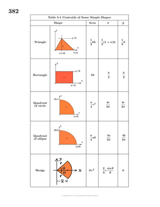
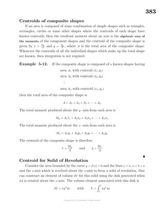
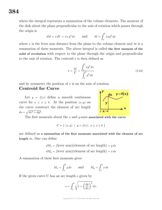
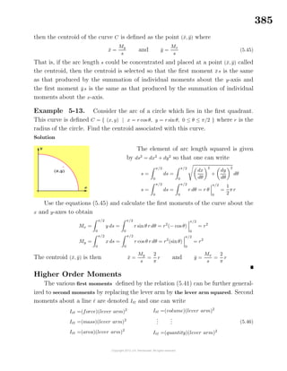
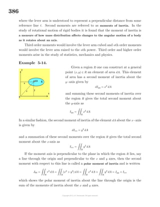
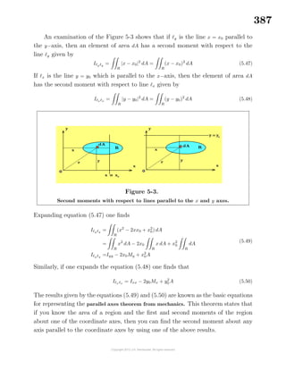
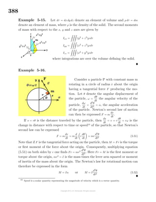
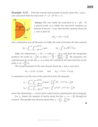
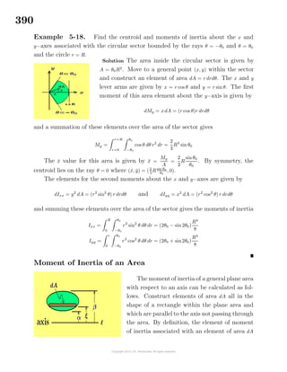
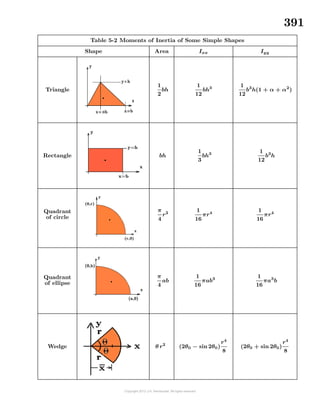
![393
Moment of Inertia of Composite Shapes
To calculate the moment of inertia of a composite area about a selected axis
(i) Calculate the moment of inertia of each component about the selected axis.
(ii) Next one need only sum the moments of inertia calculated in step (i) to calculate
the moment of inertia of the given composite area.
That is, the moment of inertia of a composite area about an axis is equal to the
sum of the moments of the component areas with respect to the same axis. Note that
if a component of the shape is removed, then this places a hole in the composite
shape and in this case the moment of inertia of the component removed is then
subtracted from the total sum.
Pressure
The average density ρ of a substance is defined as its mass m divided by its
volume V or ρ = m
V
, where [ρ] = kg/m3
, [m] = kg, [V ] = m3
. The relative density of a
substance is defined as the ratio of density of substance divided by the density of
water. Pressure is a scalar quantity defined as the average force per unit of area and
its unit of measurement is the Pascal, abbreviated (Pa), where 1 Pa = 1 Nm−2
.
Liquid Pressure
Integration can be used to determine the forces acting on submerged objects.
Pressure at a point is p = lim
∆A→0
∆F
∆A
, and represents a derivative of the force with
respect to area. An area submerged in water experiences only a pressure normal to
its surface and there are no forces parallel to the area. This is known as Pascal’s
law. Knowing the pressure at a point, one can use integration to calculate the total
force acting on a submerged object. The pressure p representing force per unit of
area must be known when constructing water-towers, dams, locks, reservoirs, ships,
submarines, under-water vessels as the total force acting on a submerged object
must be known for certain design considerations.
Consider two points P1 and P2 beneath a fluid having a constant density ρ. If
∆h = |P1 − P2| is the distance between the points and ρ is the constant density of the
liquid, then the change in pressure between the points P1 and P2 is given by
∆p = ρ g ∆h (5.57)
where h, [h] = m, is measured positive in the downward direction, ρ, [ρ] = kg/m3
,
is the density and g, [g] = m/s2
is the acceleration of gravity so that [p] = N/m2
.
Defining w = ρ g, [w] = N/m3
as the weight of the liquid per unit volume, one can](https://image.slidesharecdn.com/calculusvolume-1-160216221448/85/Calculus-volume-1-401-320.jpg)
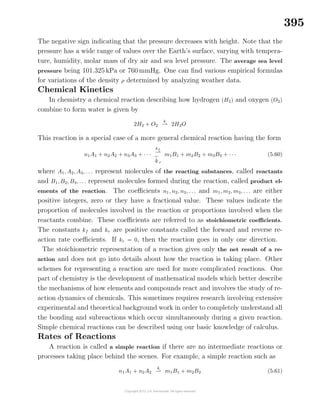
![396
states that n1 molecules of A1 and n2 molecules of A2 combined to form m1 molecules
of B1 and m2 molecules of B2. Let [A1], [A2], [B1], [B2] denote respectively the concen-
trations of the molecules A1, A2, B1, B2 with the concentration measured in units of
moles/liter. The stoichiometric reaction (5.61) states that as the concentrations of
A1 and A2 decrease, then the concentrations of B1 and B2 increase. It is assumed
that A1 and A2 decrease at the same rate so that
−
1
n1
d[A1]
dt
= −
1
n2
d[A2]
dt
(5.62)
and the concentrations of B1 and B2 increase at the same rate so that
1
m1
d[B1]
dt
=
1
m2
d[B2]
dt
(5.63)
Equating the equations (5.62) and (5.63) gives
−
1
n1
d[A1]
dt
= −
1
n2
d[A2]
dt
=
1
m1
d[B1]
dt
=
1
m2
d[B2]
dt
(5.64)
Here a standard rate of reaction is achieved by taking the rate of change of each
substance and dividing by its stoichiometric coefficient. Also note that the minus
signs are used to denote a decrease in concentration and a plus sign is used to denote
an increase in concentration.
The Law of Mass Action
There are numerous and sometimes complicated rate laws for describing the
chemical kinetics of a reaction. These complicated rate laws are avoided in presenting
this introduction to chemical kinetics. For simple chemical reactions at a constant
temperature which have the form of equation (5.60), let x = x(t) denote the number
of molecules per liter which have reacted after a time t. Many of these simple
equations obey the law of mass action which states that the rate of change of x = x(t)
with respect to time t can be represented
dx
dt
= k[A1]n1
[A2]n2
[A3]n3
· · · (5.65)
Each of the superscripts n1, n2, n3, . . . have known values and k is a rate or velocity
coefficient having units of 1/time. The order of the chemical reaction is represented
by the sum n1 + n2 + n3 + · · · of these exponents. If the sum is one, the reaction is
called a first-order reaction or unimolecular reaction. If the sum is two, the reaction
is called a second-order reaction or bimolecular. If the sum is three, the reaction is](https://image.slidesharecdn.com/calculusvolume-1-160216221448/85/Calculus-volume-1-404-320.jpg)
![397
called a third-order reaction or trimolecular, etc. Note that trimolecular and higher
order reactions are rare.
An example of a unimolecular reaction is a substance disintegrating and this
type of reaction can be represented
−
d[A]
dt
= k[A], [A] = [A](t) (5.66)
and this equation is a way of stating that the rate of change of a decaying substance
is proportional to the amount present. The proportionality constant k being called
the rate coefficient. Separate the variables in equation (5.66) and write
d[A]
[A]
= −k dt
and then integrate both sides from 0 to t, assuming that at time t = 0, [A](0) = [A]0
is the initial concentration. One can then write
[A]
[A]0
d[A]
[A]
= −k
t
0
dt
and then these equations can be integrated to obtain
ln [A] − ln [A]0 = −kt =⇒ [A] = [A](t) = [A]0 e−kt
(5.67)
where the reaction rate k has dimensions of 1/time. Use equation (5.67) and plot
[A](t) versus t one finds the result is a straight line on semi-log paper. A second-order
reaction or bimolecular reaction has the form
A1 + A2
kf
k r
B1 (5.68)
and represents a reversible bimolecular reaction. Here kf is the forward rate constant
and kr is the reverse rate constant. One can alternatively write the forward and
reverse reactions as two separate equations. If kr = 0, then there is no reverse
reaction. Apply the law of mass action to the stoichiometric reaction (5.68) gives
the differential equations
d[A1]
dt
=kr[B1] − kf [A1][A2]
d[A2]
dt
=kr[B1] − kf [A1][A2]
d[B1]
dt
= − kr[B1] + kf [A1][A2]
(5.69)
Note that the rate coefficients kr and kf can have very large differences in magnitudes
thus driving the reaction more in one direction than the other and for the reaction](https://image.slidesharecdn.com/calculusvolume-1-160216221448/85/Calculus-volume-1-405-320.jpg)
![398
(5.68) the rate coefficients kf and kr do not have the same units of measurements.
To show this one should perform a dimensional analysis on each of the terms in the
equations (5.69). Each group of terms in equation (5.69) must have the same units of
measurements so that by examining the dimensions of each term in a group one can
show the reaction rates kf and kr do not have the same dimensions. For example, if
the concentrations are measured in units of mol/liter, then the terms on the left-hand
side of the equations (5.69) all have units of mol/liter per second and consequently
each group of terms on the right-hand side of the equations (5.69) must also have this
same unit of measurement. This requires that kr have units of 1/second and kf have
units of 1
mol
liter
· second
. If different units of measurement are used one must perform
a similar type of analysis of the dimensions associated with each group of terms.
The requirement that each group of terms have the same dimensions is known as
requiring that the equations be homogeneous in their dimensions. If an equation is
not dimensionally homogeneous, then you know it is wrong.
In the equations (5.69) let kr = 0 to obtain
d[A1]
dt
= − kf [A1][A2]
d[A2]
dt
= − kf [A1][A2]
d[B1]
dt
= kf [A1][A2]
(5.70)
Let y = y(t) = [B1] denote the concentration of B1 as a function of time t. If at time
t = 0 the concentrations of A1 and A2 are denoted by [A1]0 and [A2]0, then after a
time t one can express the amount of A1 and A2 by using the equations
[A1] = [A1](t) = [A1]0 − y and [A2] = [A2](t) = [A2]0 − y
Substituting these values into the last of the equations (5.70) gives the result
dy
dt
= kf ([A1]0 − y)([A2]0 − y) (5.71)
Let α1 = [A1]0 and α2 = [A2]0 and assume α1 = α2 so that equation (5.71) can be
expressed in the form
dy
(α1 − y)(α2 − y)
= kf dt (5.72)](https://image.slidesharecdn.com/calculusvolume-1-160216221448/85/Calculus-volume-1-406-320.jpg)
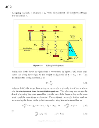
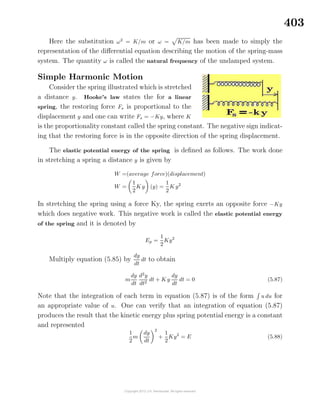
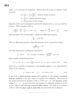
![405
Note that equations (5.91) differ only by a phase constant, since one can write
A sin(ωt + θ0) =A cos(ωt + θ0 − π/2) = A cos(ωt + φ0), φ0 = θ0 − π/2
A cos(ωt + θ0) =A sin(ωt + θ0 + π/2) = A sin(ωt + ψ0), ψ0 = θ0 + π/2
In general, given an equation of the form
y = y(t) = A1 cos ωt + A2 sinωt
one can multiply both the numerator and denominator by A2
1 + A2
2 to obtain
y = y(t) = A2
1 + A2
2
A1
A2
1 + A2
2
cos ωt +
A2
A2
1 + A2
2
sin ωt
so that the oscillatory motion can be expressed in the following form.
y =y(t) = A [sin θ0 cos ωt + cos θ0 sin ωt]
y =y(t) = A sin(ωt + θ0)
Simple harmonic motion can be characterized by observing that the acceleration
d2
y
dt2
satisfies the conditions
(i) It is always proportional to its distance from a fixed point
d2
y
dx2
= −ω2
y .
(ii) It is always directed toward the fixed point.
Damping Forces
Observe the sign of the spring force in equation (5.85). If y > 0, the restoring force
is in the negative direction. If y < 0, the restoring force is in the positive direction.
The directions of the forces are important because forces are vector quantities and
must have both a magnitude and a direction. The direction of the forces is one check
that the problem is correctly modeled.
If additional forces are added to the spring mass system, such as damping forces
and external forces, then equation (5.85) must be modified to include these addi-
tional forces. In figure 5-5, assume a damper and an external force are attached to
the spring as illustrated.](https://image.slidesharecdn.com/calculusvolume-1-160216221448/85/Calculus-volume-1-413-320.jpg)
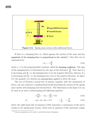
![407
term and for the equation to be dimensionally homogeneous, every term must have
dimensions of force. The quantity m¨y is called the inertial force, β ˙y is the damping
force, Ky is the spring force and F(t) is an external force. Here m, β and K are all
positive constants with dimensions [m] =
[W]
[g] = lbs
ft/sec2
, [β] = lbs
ft/sec
, [K] = lbs
ft
with
y and t having the dimensions [y] = ft and [t] = seconds. It is left as an exercise to
verify that the equation (5.94) is dimensionally homogeneous.13
To solve the differential equation (5.94) one first solves the homogeneous equa-
tion
m
d2
y
dt2
+ β
dy
dt
+ Ky = 0 (5.95)
by finding a set of two independent solutions {y1(t), y2(t)} called a fundamental set
of solutions to the homogeneous differential equation. The general solution to the
homogeneous differential equation is then any linear combination of the solutions
from the fundamental set. The general solution to equation (5.95) can be expressed
yc = c1y1(t) + c2y2(t) where c1, c2 are arbitrary constants. (5.96)
This general solution is called the complementary solution and is usually denoted
using the notation yc. Any solution of the nonhomogeneous differential equation
(5.94) is denoted using the notation yp and is called a particular solution. The general
solution to the differential equation (5.94) can then be expressed as y = yc + yp.
If the homogeneous differential equation has constant coefficients, one can assume
an exponential solution y = exp(γt) = eγt
, γ constant, to obtain the fundamental set
of solutions.
Example 5-19. Solve the differential equation
d2
y
dt2
+ 3
dy
dt
+ 2y = 2e−3t
Solution Assume an exponential solution y = eγt
to the homogeneous differential
equation
d2
y
dt2
+ 3
dy
dt
+ 2y = 0 (5.97)
and substitute y = eγt
, dy
dt
= γeγt
, d2
y
dt2 = γ2
eγt
into the homogeneous differential equa-
tion (5.97) to obtain the algebraic equation
γ2
+ 3γ + 2 = (γ + 2)(γ + 1) = 0 (5.98)
13
The word homogeneous is used quite frequently in the study of differential equations and its meaning depends
upon the context in which it is used.](https://image.slidesharecdn.com/calculusvolume-1-160216221448/85/Calculus-volume-1-415-320.jpg)
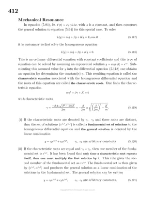
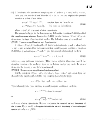
![414
Figure 5-6. Damped oscillations.
The solution equation (5.124) denotes a
damped oscillatory solution which can be vi-
sualized by plotting the curves
y1 = c2
1 + c2
2 e−βt/2m
and y2 = −y1
as envelopes of the oscillation cos(ω0t − φ) as
is illustrated in figure 5-6. The term −β/2m
is called the damping constant or damping
factor.
CASE III (Homogeneous equation and critical damping) If (β/2m)2
−K/m = 0, equation
(5.119) has the repeated roots γ1 = γ2 = −β/2m which produces the solution
yc = (c1 + c2t)e−βt/2m
. (5.125)
By reducing the damping constant β one gets to a point where oscillations begin
to occur. The motion is then said to be critically damped. The critical value for
the damping constant β in this case is denoted by βc and is determined by setting
the discriminant equal to zero to obtain βc = 2mω where ω = K/m is the natural
frequency of the undamped system.
Particular Solution
Associated with the complementary solution from one of the cases I, II, or III,
is the particular solution of the nonhomogeneous equation (5.117). The particular
solution can be determined by the method of undetermined coefficients. Examine the
function(s) on the right-hand side of the differential equation and all the derivatives
associated with these function(s). Select the basic terms which keep occurring in the
function and all of its derivatives and form a linear combination of these basic terms.
For the equation (5.117) the basic terms which occur by continued differentiation
of the right-hand side are the functions {cos λt, sin λt} multiplied by some constant.
One can then assume that the particular solution is of the form
yp = A cos λt + B sinλt (5.126)
with A and B unknown constants to be determined. Substituting this assumed par-
ticular solution into the differential equation (5.117) produces the equation
[(K − mλ2
)A + βλB] cos λt + [−βλA + (K − mλ2
)B] sinλt = F0 cos λt (5.127)](https://image.slidesharecdn.com/calculusvolume-1-160216221448/85/Calculus-volume-1-422-320.jpg)
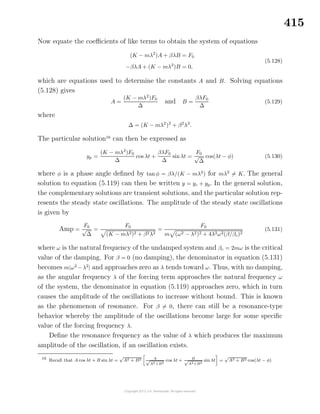
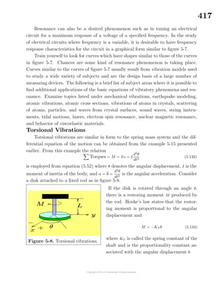
![418
From the relation in equation (5.133) there results
M = −KT θ = I
d2
θ
dt2
or I
d2
θ
dt2
+ KT θ = 0 (5.135)
as the equation of motion describing the angular displacement θ.
By adding a linear damper and external force to equation (5.135), a more general
equation results
I
d2
θ
dt2
+ β
dθ
dt
+ KT θ = F(t). (5.136)
From strength of materials, the constant KT is given by the relation KT = GJ/L,
where G is called the shearing modulus of the rod material, J is the polar moment
of inertia of the rod cross section, and L is the length of the shaft.
The simple pendulum
For the pendulum illustrated the forces about 0 are the weight
of the mass and the radial force along the string. The radial
force passes through the origin and so does not produce a mo-
ment about the origin. The moment of inertia of the mass m
about 0 is given by I = m 2
and the torque about 0 is given by
T = −(mg)( sinθ)and consequently the equation of motion can
be expressed T = −mg sinθ = m 2 d2
θ
dt2
Simplification reduces the equation of motion to the form
d2
θ
dt2
+ ω2
sin θ = 0, ω2
=
g
For small oscillations one can make the approximation sinθ ≈ θ and write the equation
for the oscillating pendulum in the form
d2
θ
dt2
+ ω2
θ = 0
which is the equation of a simple harmonic oscillator.
Electrical Circuits
The basic elements needed to study electrical circuits are as follows:
(a) Resistance R is denoted by the symbol
The dimension of resistance is ohms17
and written [R] = ohms.
17
George Simon Ohm (1787–1854), German physicist.](https://image.slidesharecdn.com/calculusvolume-1-160216221448/85/Calculus-volume-1-426-320.jpg)
![419
(b) Inductance L is denoted by the symbol
The dimension of inductance is henries18
and written [L] = henries.
(c) Capacitance C denoted by the symbol
The dimension of capacitance is farads19
and written [C] = farads.
(d) Electromotive force (emf) E or V denoted by the symbols or
The dimensions of electromotive force is volts20
and written [E] = [V ] = volts.
(e) Current I is a function of time, denoted I = I(t), with dimensions of amperes21
and written [I] = amperes.
(f) Charge Q on the capacitance is a function of time and written Q = Q(t),
with dimensions [Q] = coulombs.
The basic laws associated with electrical circuits are as follows: The current is
the time rate of change of charge. This can be represented with the above notation
as
I =
dQ
dt
with [I] = amperes, [
dQ
dt
] = coulombs/second (5.137)
Figure 5-9.
Voltage drop VR across a resistor.
Figure 5-10.
Voltage drop VL across inductor.
The voltage drop VR across a resistance, see figure 5-9, is proportional to the
current through the resistance. This is known as Ohm’s law. The proportionality
18
Joseph Henry (1797–1878), American physicist.
19
Michael Faraday (1791– 1867) English physicist.
20
Alessandro Volta (1745–1827) Italian scientist.
21
Andr´e Marie Amp´ere (1775–1836) French physicist.](https://image.slidesharecdn.com/calculusvolume-1-160216221448/85/Calculus-volume-1-427-320.jpg)
![420
constant is called the resistance R. In symbols this can be represented as VR = RI
where
[VR] = volts = [R][I] = (ohm) (ampere) (5.138)
The voltage drop VL across an inductance, see figure 5-10, is proportional to the
time rate of change of current through the inductance. The proportionality constant
is called the inductance L. In symbols this can be represented as
VL = L
dI
dt
where [VL] = volts = [L] [
dI
dt
] = (henry)(ampere/second) (5.139)
Figure 5-11.
Voltage drop VC across capacitor.
The voltage drop VC across a capacitance, see
figure 5-11, is proportional to the charge Q of
the capacitance. The proportionality constant
is denoted 1/C. In symbols this is represented
as
VC =
Q
C
(5.140)
where [VC ] = volts =
1
C
[Q] = coulombs/farad
The Kirchoff laws for an electric circuit are.
Kirchhoff’s22
first law :
The sum of the voltage drops around a closed circuit must equal zero.
Kirchhoff’s second law:
The amount of current into a junction must equal the current leaving the junc-
tion.
The place in an electrical circuit where two or more circuit elements are joined
together is called a junction. A closed circuit or loop occurs whenever a path con-
structed through connected elements within a circuit closes upon itself. Voltage
drops are selected as positive, whereas voltage rises are selected as negative.
Example 5-22. For the RC-circuit illustrated in figure 5-12, set up the differ-
ential equation describing the rate of change of the charge Q on the capacitor. Make
the assumption that Q(0) = 0.
22
Gustav Robert Kirchhoff (1924–1887) German physicist.](https://image.slidesharecdn.com/calculusvolume-1-160216221448/85/Calculus-volume-1-428-320.jpg)
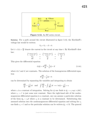
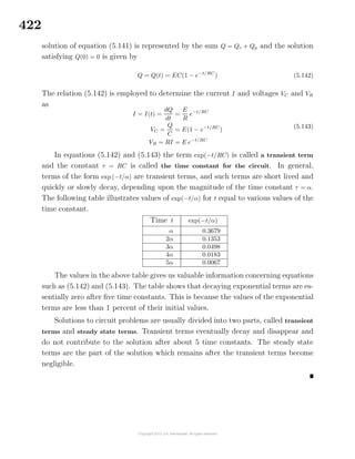
![424
Thermodynamics
Experiments on a fixed mass of gas has established the following gas laws which
relate the pressure P, volume V and absolute temperature T.
Boyle’s Law If T is held constant, then pV = constant.
Charles’s Law If P is held constant, then
V
T
= constant.
Gay-Lussac Law If V is held constant, then
P
T
= constant.
These laws are summarized using the gas equation
P1V1
T1
=
P2V2
T2
where pressure P can be measured in units [N/m2
], volume V can be measured in
units [m3
] and absolute temperature T is measured in units [K].
The ideal gas absolute temperature is defined using Boyles law which states
PV ∝ T which produces the equation of state for an ideal gas, which can be expressed
in the form
PV =nRT
[
N
m2
][m3
] =[mol]
J
mol K
[K]
where n is the number of moles of gas and R = 8.314472 J
mol K is the ideal gas constant
or universal molar gas constant. Note that real gases may or may not obey the ideal
gas law. For gases which are imperfect, there are many other proposed equations of
state. Some of these proposed equations are valid over selected ranges and conditions
and can be found under such names as Van der Waals equation, Berthelot equation,
Dieterici equation, Beattie-Bridgeman equation, Virial equation.
The zeroth law of thermodynamics states that if two bodies are in thermal equi-
librium with a third body, then the two bodies must be in thermal equilibrium with
each other. The zeroth law is used to develop the concept of temperature. Here
thermodynamic equilibrium infers that the system is (i) in chemical equilibrium and
(ii) there are no pressure or temperature gradients which would cause the system
to change with time. The first law of thermodynamics is an energy conservation
principle which can be expressed dQ = dU + dW where dQ is the heat supplied to
a gas, dU is the change in internal energy of the gas and dW is the external work
done. The second law of thermodynamics examines processes that can happen in
an isolated system and states that the only processes which can occur are those for
which the entropy either increases or remains constant. Here entropy S is related](https://image.slidesharecdn.com/calculusvolume-1-160216221448/85/Calculus-volume-1-432-320.jpg)
![425
to the ability or inability of a systems energy to do work. The change in entropy is
defined as dS = dQ/T where dQ is the heat absorbed in an isothermal and reversible
process and T denotes the absolute temperature.
Recall that the ability of gases to change when subjected to pressure and tem-
perature variations can be described by the equation of state of an ideal gas
PV = nRT, (5.146)
where P is the pressure [N/m2
], V is the volume [m3
], n is the amount of gas [moles], R
is the universal gas constant [J/mol · K], and T is the temperature [K]. For an ideal
gas, the gas constant R can also be expressed in terms of the specific heat at constant
pressure Cp, [J/mol · K] and the specific heat at constant volume Cv, [J/mol · K] by
Mayer’s equation R = Cp − Cv. Equation (5.146) is illustrated in the pressure-volume
diagram of figure 5-14.
The curves where T is a constant are called isothermal curves and are the hy-
perbolas labeled (b) and (c) illustrated in figure 5-14. These curves correspond to
the temperature values T1 and T2. When a gas undergoes changes of state it can do
so by an isobaric process (P is a constant) illustrated by line (a) in figure 5-14, an
isovolumetric process (V is a constant) illustrated by the line (e) in figure 5-14, an
isothermal process (T is a constant) illustrated by the hyperbolas with T = T1 and
T = T2 in figure 5-14, or an adiabatic process (no heat is transferred) represented by
the curve (d) in figure 5-14.
Figure 5-14. Pressure-Volume diagram.](https://image.slidesharecdn.com/calculusvolume-1-160216221448/85/Calculus-volume-1-433-320.jpg)
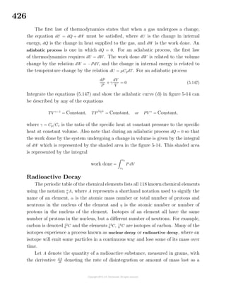
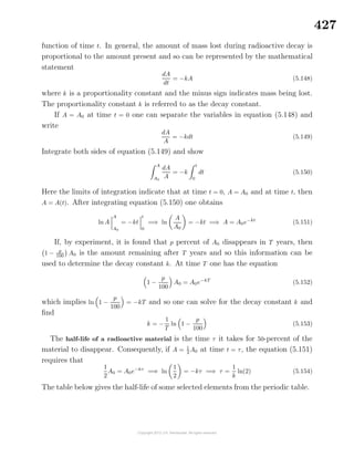
![430
(i) The minus sign in the representation for r indicates that an increase in the
selling price will cause a decrease in sales. This can be seen by plotting the
curve x = α
β
− 1
β
r versus r which is a straight line with slope −1/β. This line tells
one that as r increases (price increases), then the number of sales x decreases.
(ii) The constant α has to be large enough such that α − βx remains positive as you
don’t want to give away the product.
(iii) In the cost function, the constant a represents the overhead for the maintenance
of the production facilities and the variable term bx represent the additional cost
of production associated with producing x units. The units of measurements for
each term must be in dollars so [a] = $ and [b] = $/unit and [x] = number of units.
Hence, one can interpret b as the cost to produce 1 unit.
Using the above assumptions the profit from the sale of x items is given by
P = P(x) = x(α − βx) − (a + bx)
and if a profit is to be made from the sale of just one item, then it is required that
α > β + a + b. The derivative of the profit with respect to x is
dP
dx
= x(−β) + (α − βx) − b
The profit is a maximum when
dP
dx
= 0 or x =
α − b
2β
is a critical point to be investi-
gated. The second derivative gives
d2
P
dx2
= −2β < 0 indicating that the critical point
produces a maximum value. These results are interpreted
(i) x =
α − b
2β
items should be produced for a maximum profit.
(ii) The sale price for each item should be r =
α + b
2
dollars per unit.
In economics the term R(x) = x·r(x) is called the revenue function and its deriva-
tive dR
dx
is called the marginal revenue. The term P(x) is called the profit function
and its derivative dP
dx
is called the marginal profit. The term C(x) is called the cost
function and its derivative dC
dx
is called the marginal cost function.
By collecting data from production costs and sales over a period of time one can
construct better approximations for the price function and cost function and other
models similar to the above can be constructed and analyzed.](https://image.slidesharecdn.com/calculusvolume-1-160216221448/85/Calculus-volume-1-438-320.jpg)
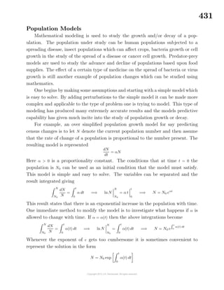
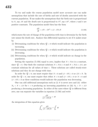
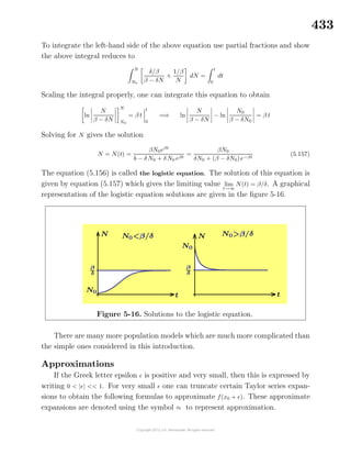
![434
(1 + )n
≈ 1 + n
1
1 +
≈ 1 −
1
√
1 +
≈ 1 −
2
sin ≈ −
3
3!
cos ≈ 1 −
2
2!
tan ≈ +
3
3
a ≈ 1 + lna
e ≈ 1 +
ln(x + ) ≈ ln x +
x
It is left as an exercise to verify the above approximations.
Partial Differential Equations
Examples of partial differential equations can be found in just about all of the
scientific disciplines. For example, partial differential equations are employed to
describe such things as fluid motion, quantum mechanical interactions, diffusion
processes, wave motion and electric and magnetic phenomena. The following are
some examples of partial differential equations. The derivation of these well known
partial differential equations are presented in more advanced courses.
The vibrating string
Let u = u(x, t) denote the displacement of a
string at position x and time t, where the string
is stretched between the points (0, 0) and (L, 0).
The assumption that T, the tension in the string,
is much greater than the weight of the string,
produces the equation describing the vibrations of the string. The partial differential
equation describing the vibrations of the string is given by
∂2
u
∂t2
= ω2 ∂2
u
∂x2
, u = u(x, t), ω2
=
Tg
ρ
where T is the string tension, g the acceleration of gravity and ρ is the weight per
unit length of string. This equation is called the one-dimensional wave equation and
is subject to boundary conditions u(0, t) = 0 and u(L, t) = 0 and initial conditions
u(x, 0) =f(x) = the initial shape of the string
and
∂u(x, 0)
∂t
=g(x) = the initial velocity of the string
The above quantities have the following dimensions [x] = cm, [t] = s, [u] = cm,
[ρ] = gm/cm, [T] = dynes/cm and [g] = cm/sec2
.
The above one-dimensional wave equation is a special case of a more general
three-dimensional wave equation.](https://image.slidesharecdn.com/calculusvolume-1-160216221448/85/Calculus-volume-1-442-320.jpg)
![435
One-dimensional heat flow
The partial differential equation describing the one-dimensional heat flow in a
rod along the x-axis is given by
k
∂2
T
∂x2
= cρ
∂T
∂t
, T = T(x, t)
where T = T(x, t) is the temperature at position x and time t in an insulated rod of
length L, where k is called the thermal conductivity of the solid, ρ is the volume
density of the solid and c is the specific heat of the solid. The above quantities have
the following dimensions [x] = cm, [t] = s, [T] = ◦
C, [c] = cal/gm◦
C , [ρ] = gm/cm3
and
[k] = cal/seccm2 ◦
C/cm.
The one-dimensional heat equation is a special case of the more general three-
dimensional diffusion equation.
Easy to Solve Partial Differential Equations
Partial differential equations of the form
∂u
∂x
= f(x, y)
can be integrated partially with respect to x to obtain
∂u
∂x
dx = f(x, y) dx =⇒ u(x, y) = f(x, y) dx + φ(y)
Here, y is held constant during the integration process and so the constant of inte-
gration can be any arbitrary function of y, represented here by φ(y).
Similarly, the partial differential equation
∂u
∂y
= g(x, y)
can be integrated partially with respect to y to obtain
∂u
∂y
dy = g(x, y) dy =⇒ u(x, y) = g(x, y) dy + ψ(x)
Here x is held constant during the integration process and so any arbitrary func-
tion of x is considered as a constant of integration. This constant of integration is
represented by ψ(x).](https://image.slidesharecdn.com/calculusvolume-1-160216221448/85/Calculus-volume-1-443-320.jpg)
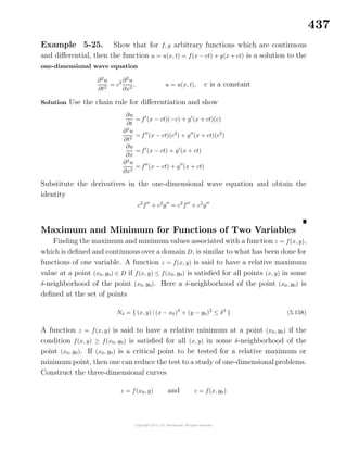
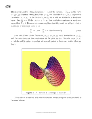
![439
Exercises
5-1. Consider a spherical balloon at the instant when the radius of the balloon is
r0 [cm]. If air is entering the balloon at the rate of α [cm3
/s], then at what rate is
the radius of the balloon changing at this instant?
5-2. Air expands adiabatically (no heat loss or gain) according to the gas law
pv1.4
= constant, where p is the pressure [dyne/cm2
] and v is the volume [cm3
].
(a) If the volume is increasing at a rate α [cm3
/s], then find the corresponding rate
of change in pressure.
(b) If the pressure is decreasing at a rate β [dyne/cm2
s] then find the corresponding
rate of change in the volume.
5-3. A women who is 5.5 feet tall walks away from a street lamp, where the lamp
is 10 feet above the ground. She walks at a rate of 4 ft/s
(a) At what rate is her shadow changing when she is 4 feet from the lamp post?
(b) Is the length of shadow increasing or decreasing as she walks away from the
lamp?
(c) At what instant is the shadow 5.5 feet long?
5-4. For a thin lens in air, let x denote the distance of the object from the lens
and let y denote the distance of the image from the lens. The distances x and y are
related by the thin lens formula
1
x
+
1
y
=
1
f
where f is a constant representing the
focal length of the lens.
(a) Show the thin lens formula can be written
in the Newtonian form S1S2 = f2
where
S1 = x − f > 0 and S2 = y − f > 0.
(b) If x changes at a rate
dx
dt
= r0, then find a
formula for the rate of change of y.
5-5. The sides of an equilateral triangle increase at the rate of r0 cm/hr. Find a
formula for the rate of change of the area of an equilateral triangle when the length
of a side is x0 cm.](https://image.slidesharecdn.com/calculusvolume-1-160216221448/85/Calculus-volume-1-447-320.jpg)
![440
5-6. A meteorologist, at a secret location, collects data and comes up with an
atmospheric pressure formula p = p0 e−α0h
where [p] = lbs/ft2
, h has dimensions of feet
and represents the altitude above sea-level. In the atmospheric pressure formula the
quantities p0 and α0 are known constants.
(a) Find the dimensions of the constants p0 and α0.
(b) If the meteorologist gets into a balloon which rises at a rate of 10 ft/s, then find
a formula representing the rate of change in the pressure when the altitude is h0
feet.
5-7. Given the parabola y − y0 = −(x − x0)2
where x0, y0
are known constants.
(a) At the point (ξ, η) on the curve a tangent line is
constructed. Find the equation of the tangent
line.
(b) The tangent line makes an angle θ with the x-
axis as illustrated. If ξ changes at the rate of 1/2
cm/s, then at what rate does θ change?
5-8. Charles23
law, sometimes referred to as the law of volumes, states that at a
constant pressure the volume V of a gas and gas temperature T satisfy the relation
V
T
= C = constant, where V is the volume of the gas in cubic centimeters and T
is the absolute temperature in degrees Kelvin. If at a certain instant when V has
the volume V0 and T has the temperature T0, it is know that the volume of gas is
changing at the rate
dV
dt
= r0, then find how the temperature is changing.
5-9. The Gay-Lussac24
law states that if the mass and volume of an ideal gas
are held constant, then the pressure of the gas varies directly with the gas absolute
temperature. If P denotes pressure measured in Pascals and T is the absolute temper-
ature in degrees Kelvin, then the Gay-Lussac law can be expressed
P
T
= C = constant.
If at some instant when P has the value P0 and T has the value T0, it is known that
the temperature is change at the rate
dT
dt
= r0, then find how the pressure is changing
at this instant.
23
Jacques Charles (1746-1823) French physicist and physical chemist as well as a balloonist.
24
Joseph Louis Gay-Lussac (1778-1850) A French chemist who studied the expansion of gases.](https://image.slidesharecdn.com/calculusvolume-1-160216221448/85/Calculus-volume-1-448-320.jpg)
![441
5-10. A rock is thrown off a cliff so that after a time t its height above the ground
is h = h(t) = 200 − 16t2
.
(a) Find a formula representing the velocity of the rock.
(b) Find a formula representing the acceleration of the rock.
(c) What is the rocks velocity when it hits the ground?
5-11.
A spherical water tank has a radius of r = 12 feet. As-
sume h = h(t) is the depth of the water in the spherical
tank. The empty space above the water level inside
the tank defines a spherical cap whose volume is given
by Vcap = π
3
(2r − h)2
(r + h)
(a) Show the volume of water in the spherical tank is given by V = V (h) = π
3
(3rh2
−h3
)
(b) If water is entering the tank at 10 gallons per minute, then how fast is the water
level rising when h = 10 feet? Hint: Use 1 gallon =0.1336 cubic feet.
5-12. A spherical water tank has radius of r = 12 feet. Assume that h = h(t) is the
depth of the water in the spherical water tank and R = R(t) is the radius of the top
surface of the water. Find a relationship between dh
dt
and dR
dt
.
5-13. A ball is shot from an air gun inclined at an angle θ with the horizontal.
The height of the ball as a function of time is given by y = y(t) = −16t2
+ 50
√
3t and
the horizontal distance traveled is given by x = x(t) = 50t.
Answer the following questions.
(a) Find the maximum height of the ball.
(b) Find the time when the maximum height is achieved.
(c) Find the time when the ball hits the ground.
(d) Find the x position where the maximum height is achieved.
(e) Eliminate time t from x = x(t) and y = y(t) to obtain y as a function of x.
5-14. Empirical data obtained by shooting bullets into maple wood blocks pro-
duces the formula
v = v(x) = K
√
1 − 2x, 0 < x < 1/2, (K is a constant )
for the speed [ft/s] of the bullet after it has penetrated the wood a distance x feet.
Find the rate at which the speed of the bullet is decreasing after it enters the wood.](https://image.slidesharecdn.com/calculusvolume-1-160216221448/85/Calculus-volume-1-449-320.jpg)

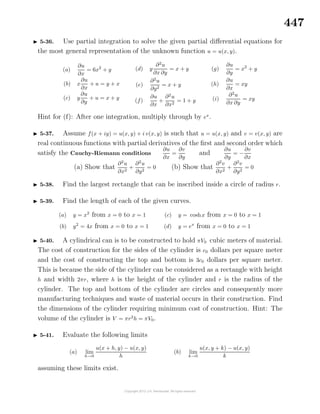
![449
5-46. The Trapezoidal Rule
Given a curve y = f(x), a ≤ x ≤ b, one can
partition the interval [a, b] into n-parts by defin-
ing a step size h = ∆x = (b−a)
n
and then labeling
the points
a = x0, x1 = x0+h, . . ., xn−1 = x0+(n−1)h, xn = x0+nh
Next construct trapezoids, the ith trapezoid has
the vertices xi−1, yi−1, xi, yi as illustrated in the
figure, where yi−1 = f(xi−1) and yi = f(xi).
(a) Show the area of the ith trapezoid is given by
Ai =
1
2
(yi−1 + yi)h =
h
2
[f(xi−1) + f(xi)]
(b) Show the area of all the trapezoids is
A = total area =
n
i=1
Ai =
n
i=1
1
2
(yi−1 + yi)h =
h
2
(y0 + yn) + 2
n−1
i=1
yi
(c) Computer Problem
For the functions given over the interval specified compare the area under
the curve using the definite integral
b
a
f(x) dx, with the trapezoidal rule for
approximating the area. Fill in the following table for values of n = 10, 50 and
100 associated with each function.
Area under curve y = f(x) for a ≤ x ≤ b
Function Interval Trapezoidal Integration
n= f(x) a ≤ x ≤ b
n
i=1 Ai
b
a
f(x) dx
x 0 ≤ x ≤ 2
x2
0 ≤ x ≤ 2
x3
0 ≤ x ≤ 2
sin x 0 ≤ x ≤ π
cos x π
2
≤ x ≤ 3π
2
(d) If the theoretical error of approximation using the trapezoidal rule is
E =
(b − a)3
12n2
f (ξ) , where a < ξ < b, compare your errors with the maximum
theoretical error.](https://image.slidesharecdn.com/calculusvolume-1-160216221448/85/Calculus-volume-1-457-320.jpg)
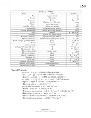
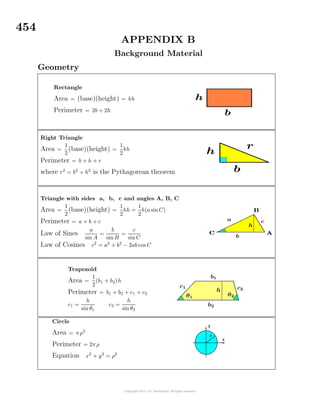
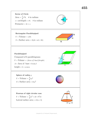
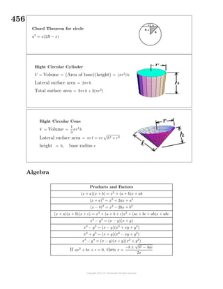
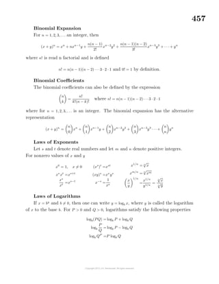
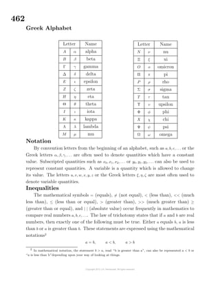
![466
Appendix C
Table of Integrals
Indefinite Integrals
General Integration Properties
1. If
dF (x)
dx
= f(x) , then f(x) dx = F (x) + C
2. If f(x) dx = F (x) + C , then the substitution x = g(u) gives f(g(u)) g (u) du = F (g(u)) + C
For example, if
dx
x2 + β2
=
1
β
tan−1 x
β
+ C, then
du
(u + α)2 + β2
=
1
β
tan−1 u + α
β
+ C
3. Integration by parts. If v1(x) = v(x) dx, then u(x)v(x) dx = u(x)v1(x) − u (x)v1(x) dx
4. Repeated integration by parts or generalized integration by parts.
If v1(x) = v(x) dx, v2(x) = v1(x) dx, . . ., vn(x) = vn−1(x) dx, then
u(x)v(x) dx = uv1 − u v2 + u v3 − u v4 + · · · + (−1)n−1
un−1
vn + (−1)n
u(n)
(x)vn(x) dx
5. If f−1
(x) is the inverse function of f(x) and if f(x) dx is known, then
f−1
(x) dx = zf(z) − f(z) dz, where z = f−1
(x)
6. Fundamental theorem of calculus.
If the indefinite integral of f(x) is known, say
f(x) dx = F (x) + C, then the definite integral
b
a
dA =
b
a
f(x) dx = F (x)]
b
a = F (b) − F (a)
represents the area bounded by the x-axis, the curve
y = f(x) and the lines x = a and x = b.
7. Inequalities.
(i) If f(x) ≤ g(x) for all x ∈ (a, b), then
b
a
f(x) dx ≤
b
a
g(x) dx
(ii) If |f(x) ≤ M| for all x ∈ (a, b) and b
a f(x) dx exists, then
b
a
f(x) dx ≤
b
a
f(x) dx ≤ M(b − a)
Appendix C](https://image.slidesharecdn.com/calculusvolume-1-160216221448/85/Calculus-volume-1-474-320.jpg)
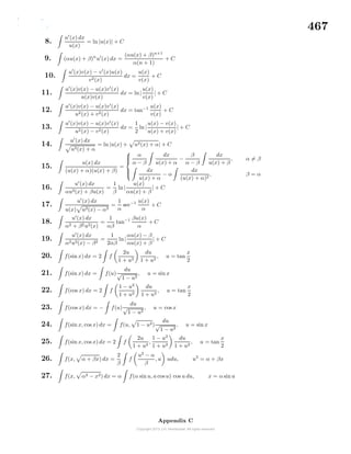
![468
General Integrals
28. c u(x) dx = c u(x) dx 29. [u(x) + v(x)] dx = u(x) dx + v(x) dx
30. u(x) u (x) dx =
1
2
| u(x) |2
+C 31. [u(x) − v(x)] dx = u(x) dx − v(x) dx]
32. un
(x) u (x) dx =
[u(x)]n+1
n + 1
+ C 33. u(x) v (x) dx = u(x) v(x) − u (x) v(x) dx
34. F [u(x)] u (x)dx = F [u(x)] + C 35.
u (x)
u(x)
dx = ln | u(x) | +C
36.
u
2
√
u
dx =
√
u + C 37. 1 dx = x + C
38. xn
dx =
xn+1
n + 1
+ C 39.
1
x
dx = ln | x | +C
40. eau
u dx =
1
a
eau
+ C 41. au
u dx =
1
lna
au
+ C
42. sin u u dx = cos u + C 43. cos u u dx = − sin u + C
44. tan u u dx = ln | sec u | +C 45. cot u u dx = ln | sin u | +C
46. sec u u dx = ln | sec u + tan u | +C 47. csc u u dx = ln | csc u − cot u | +C
48. sinh u u dx = cosh u + C 49. cosh u u dx = sinh u + C
50. tanh u u dx = lncosh u + C 51. coth u u dx = ln sinhu + C
52. sech u u dx = sin−1
(tanh u) + C 53. csch u u dx = lntanh
u
2
+ C
54. sin2
u u dx =
1
2
u −
1
4
sin 2u + C 55. cos2
u u dx =
u
2
+
1
4
sin 2u + C
56. tan2
u u dx = tan u − u + C 57. cot2
u u dx = − cot u − u + C
58. sec2
u u dx = tan u + C 59. csc2
u u dx = − cot u + C
60. sinh2
u u dx =
1
4
sinh 2u −
1
2
u + C 61. cosh2
u u dx =
1
4
sinh2u +
1
2
u + C
62. tanh2
u u dx = u − tanh u + C 63. coth2
u u dx = u − coth u + C
64. sech 2
u u dx = tanh u + C 65. csch 2
u u dx = − coth u + C
66. sec u tan u u dx = sec u + C 67. csc u cot u u dx = − csc u + C
68. sech u tanh u u dx = −sech u + C 69. csch u coth u u dx = −csch u + C
Integrals containing X = a + bx, a = 0 and b = 0
70. Xn
dx =
Xn+1
b(n + 1)
+ C, n = −1
71. xXn
dx =
Xn+2
b2(n + 2)
−
aXn+1
b2(n + 1)
+ C, n = −1, n = −2
72. X(x + c)n
dx =
b
n + 2
(x + c)n+2
+
a − bc
n + 1
(x + c)n+1
+ C
Appendix C](https://image.slidesharecdn.com/calculusvolume-1-160216221448/85/Calculus-volume-1-476-320.jpg)
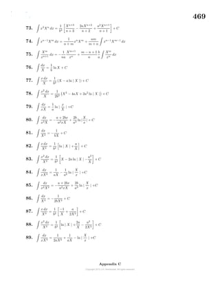
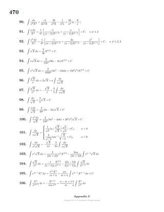
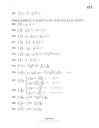
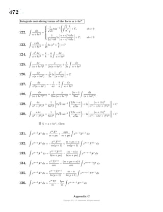
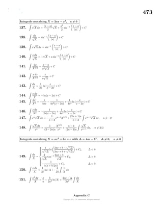
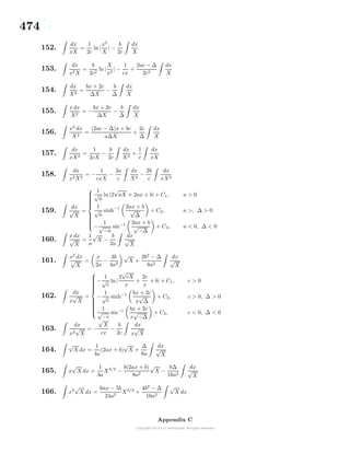
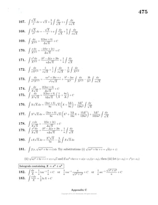
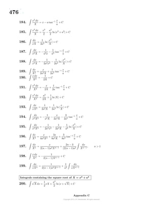
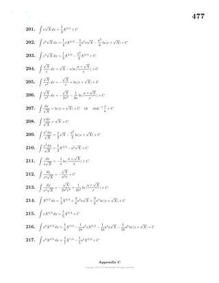
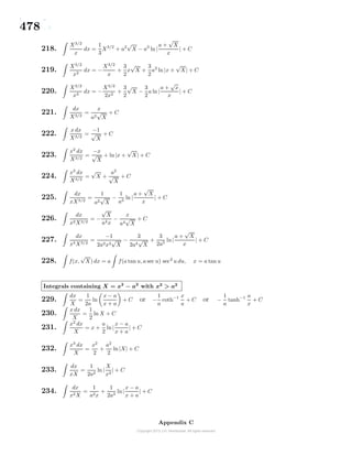
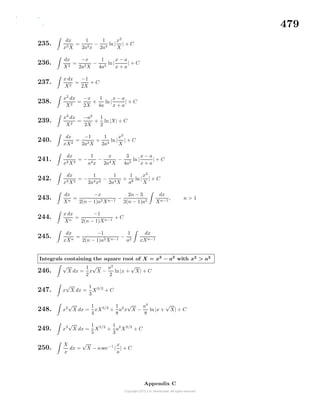
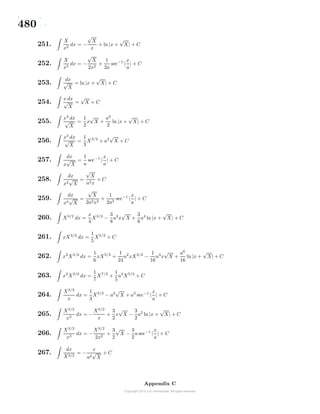
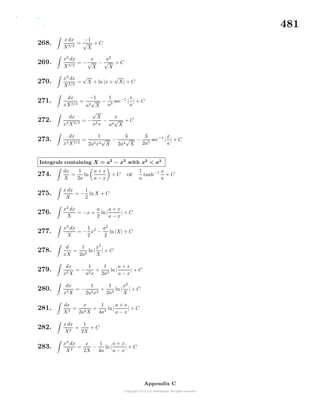
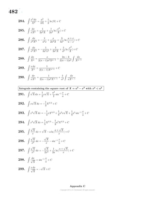
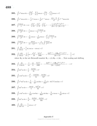
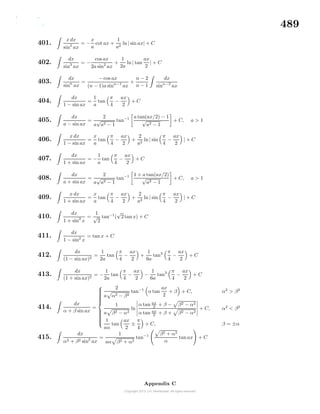
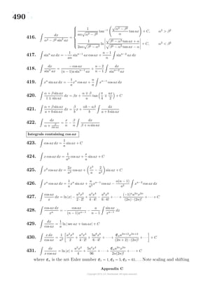
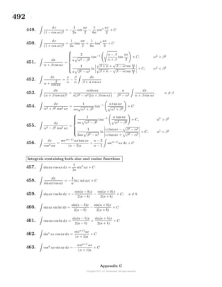
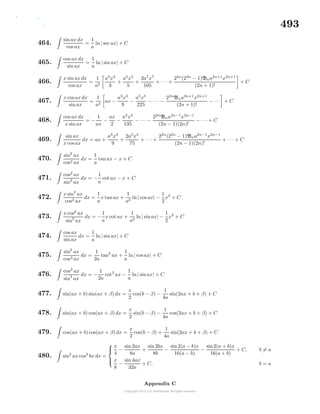
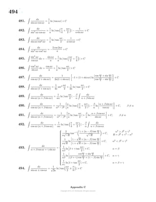
![495
495.
sinax dx
sin ax ± cos ax
=
x
2
ln | sinax ± cos ax| + C
496.
cos ax dx
sin ax ± cos ax
= ±
x
2
+
1
2a
ln | sinaxx ± cos ax| + C
497.
sin ax dx
α + β sin ax
=
1
aβ
ln|α + β sin ax| + C
498.
cos ax dx
α + β sin ax
=
1
aβ
ln|α + β sin ax| + C
499.
sin ax cos ax dx
α2 cos2 ax + β2ax
=
1
2a(β2 − α2)
ln|α2
cos2
ax + β2
sin2
ax| + C, β = α
500.
dx
α2 sin2
ax + β2 cos2 ax
=
1
aαβ
tan−1 α
β
tanax + C
501.
dx
α2 sin2
ax − β2 cos2 ax
=
1
2aαβ
ln
α tan ax − β
α tan ax + β
+ C
502.
sinn
ax
cos(n+2 ax
dx =
tann+1
ax
(n + 1)a
+ C
503.
cosn
ax
sin(n+2)
ax
dx = −
cot(n+1)
ax
(n + 1)a
+ C
504.
dx
α + β sin ax
cos ax
=
αx
α2 + β2
+
β
a(α2 + β2)
ln|β sinax + α cos ax| + C
505.
dx
α + β cos ax
sin ax
=
αx
α2 + β2
−
β
a(α2 + β2)
ln|α sin ax + β cos ax| + C
506.
cosn
ax
sinn
ax
dx = −
cot(n−1)
ax
(n − 1)a
− cot(n−2)
ax dx
507.
sinn
ax
cosn ax
dx =
tann−1
ax
(n − 1)a
−
sinn−2
ax
cosn−2 ax
dx
508.
sin ax
cos(n+1) ax
dx =
1
na
secn
ax + C
509.
α sin x + β cos x
γ sin x + δ cos x
dx =
[(αγ + βδ)x + (βγ − αγ) ln |γ sin x + δ cos x|]
γ2 + δ2
+ C
510.
α + β sin x
a + b cos x
dx =
2α
√
a2 − b2
tan−1 a − b
a + b
tan
x
2
−
β
b
ln|a + b cos x| + C, a > b
2α
√
b2 − a2
tanh−1 b − a
b + a
tan
x
2
−
β
b
ln|a + b cos x| + C, a < b
Appendix C](https://image.slidesharecdn.com/calculusvolume-1-160216221448/85/Calculus-volume-1-503-320.jpg)
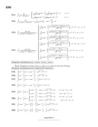
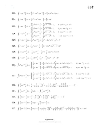
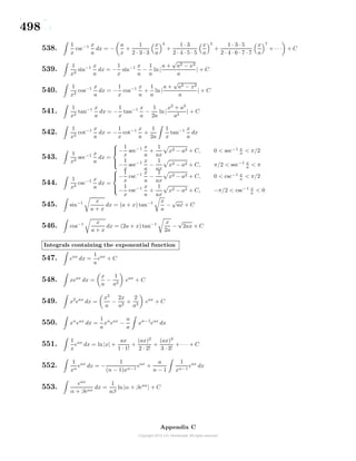
![499
554. eax
sin bx dx =
a sin bx − b cos bx
a2 + b2
eax
+ C
555. eax
cos bx dx =
a cos bx + b sin bx
a2 + b2
eax
+ C
556. eax
sinn
bx dx =
a sinbx − nb cos bx
a2 + n2b2
eax
sinn−1
bx +
n(n − 1)b2
a2 + n2b2
eax
sinn−2
bx dx
557. eax
cosn
bx dx =
a cos bx + nb sinbx
a2 + n2b2
eax
cosn−1
bx +
n(n − 1)b2
a2 + n2b2
eax
cosn−2
bx dx
Another way to express the above integrals is to define
Cn = eax
cosn
bx dx and Sn = eax
sinn
bx dx, then one can write the reduction formulas
Cn =
a cos bx + nb sin bx
a2 + n2b2
eax
cosn−1
bx +
n(n − 1)b2
a2 + n2b2
Cn−2
Sn =
a sin bx − nb cos bx
a2 + n2b2
eax
sinn−1
bx +
n(n − 1)b2
a2 + n2b2
Sn−2
558. xeax
sin bx dx =
[2ab − b(a2
+ b2
)x] cos bx + [a(a2
+ b2
)x − a2
+ b2
] sinbx
(a2 + b2)2
eax
+ C
559. xeax
cos bx dx =
[a(a2
+ b2
)x − a2
+ b2
] cos bx + [b(a2
+ b2
)x − 2ab] sinbx
(a2 + b2)2
eax
+ C
560. eax
ln x dx =
1
a
eax
ln x −
1
a
1
x
eax
dx
561. eax
sinh bx dx =
a sinh bx − b cosh bx
(a − b)(a + b)
eax
+ C, a = b
562. eax
sinh ax dx =
1
4a
e2ax
−
x
2
+ C
563. eax
cosh bx dx =
a cosh bx − b sinhbx
(a − b)(a + b)
eax
+ C, a = b
564. eax
cosh ax dx =
1
4a
e2ax
+
x
2
+ C
565.
dx
α + βeax
=
x
α
−
1
aα
ln|α + βeax
| + C
566.
dx
(α + βeax)2
=
x
α2
+
1
aα(α + βeax)
−
1
aα2
ln|α + βeax
| + C
567.
dx
αeax + βe−ax
=
1
a
√
αβ
tan−1 α
β
eax
+ C, αβ > 0
1
2a
√
−αβ
ln
eax
− −β/α
eax + −β/α
+ C, αβ < 0
Appendix C](https://image.slidesharecdn.com/calculusvolume-1-160216221448/85/Calculus-volume-1-507-320.jpg)
![501
584. x sinh ax dx =
1
a
x cosh ax −
1
a2
sinh ax + C
585. x2
sinhax dx =
x2
a
+
2
a3
cosh ax −
2x
a2
sinh ax + C
586. xn
sinh ax dx =
1
a
xn
cosh ax −
n
a
xn−1
cosh ax dx
587.
1
x
sinh ax dx = ax +
(ax)3
3 · 3!
+
(ax)5
4 · 5!
+ · · · + C
588.
1
x2
sinh ax dx = −
1
x
sinh ax + a
1
x
cosh ax dx
589.
1
xn
sinh ax dx = −
sinh ax
(n − 1)xn−1
+
a
n − 1
1
xn−1
cosh ax dx
590.
dx
sinh ax
=
1
a
ln | tanh
ax
2
| + C
591.
x dx
sinh ax
=
1
a2
ax −
(ax)3
18
+ frac7(ax)5
1800 + · · · + (−1)n 2(22n
− 1)Bn a2n+1
x2n+1
(2n + 1)!
+ · · · + C
592. sinh2
ax dx =
1
2a
x sinh2ax −
1
2
x + C
593. sinhn
ax dx =
1
na
sinhn−1
ax cosh ax −
n − 1
n
sinhn−2
ax dx
594. x sinh2
ax dx =
1
4a
x sinh 2ax −
1
8a2
cosh 2ax −
1
4
x2
+ C
595.
dx
sinh2
ax
= −
1
a
coth ax + C
596.
dx
sinh3
ax
= −
1
2a
csch ax coth ax −
1
2a
ln| tanh
ax
2
| + C
597.
x dx
sinh2
ax
= −
1
a
x coth ax +
1
a2
ln| sinh ax| + C
598. sinh ax sinh bx dx =
1
2(a + b)
sinh(a + b)x −
1
2(a − b)
sinh(a − b)x + C
599. sinh ax sin bx dx =
1
a2 + b2
[a cosh ax sin bx − b sinh ax cos bx] + C
600. sinh ax cos bx dx =
1
a2 + b2
[a cosh ax cos bx + b sinh ax sinbx] + C
Appendix C](https://image.slidesharecdn.com/calculusvolume-1-160216221448/85/Calculus-volume-1-509-320.jpg)
![503
617.
dx
cosh2
ax
=
1
a
tanh ax + C
618.
x dx
cosh2
ax
=
1
a
x tanh ax −
1
a2
ln| cosh ax| + C
619.
dx
coshn
ax
=
1
(n − 1)a
x sinh ax
coshn−1
ax
+
n − 2
n − 1
dx
coshn−2
ax, n > 1
620. cosh ax cosh bx dx =
1
2(a − b)
sinh(a − b)x +
1
2(a + b)
sinh(a + b)x + C
621. cosh ax sinbx dx =
1
a2 + b2
[a sinhax sin bx − b cosh ax cos bx] + C
622. cosh ax cos bx dx =
1
a2 + b2
[a sinh ax cos bx + b cosh ax sinbx] + C
623.
dx
α + β cosh ax
=
2
β2 − α2
tan−1 βeax
+ α
β2 − α2
+ C, β2
> α2
1
a α2 − β2
ln
βeax
+ α − α2 − β2
βeax + α + α2 − β2
+ C, β2
< α2
624.
dx
1 + cosh ax
=
1
a
tanh ax + C
625.
x dx
1 + cosh ax
=
x
a
tanh
ax
2
−
2
a2
ln| cosh
ax
2
| + C
626.
dx
−1 + cosh ax
= −
1
a
coth
ax
2
+ C
627.
dx
(α + β cosh ax)2
=
β sinh ax
a(β2 − α2)(α + β cosh ax)
−
α
β2 − α2
dx
α + β cosh ax
628.
dx
α2 − β2 cosh2
ax
=
1
2aα α2 − β2
ln
α tanh ax + α2 − β2
α tanh ax − α2 − β2
+ C, α2
> β2
−1
aα β2 − α2
tan−1 α tanh ax
β2 − α2
+ C, α2
< β2
629.
dx
α2 + β2 cosh2
ax
=
1
aα α2 + β2
tanh−1 α tanh ax
α2 + β2
+ C
Integrals containing the hyperbolic functions sinh ax and cosh ax
630. sinh ax cosh ax dx =
1
2a
sinh2
ax + C
631. sinh ax cosh bx dx =
1
2(a + b)
cosh(a + b)x +
1
2(a − b)
cosh(a − b)x + C
Appendix C](https://image.slidesharecdn.com/calculusvolume-1-160216221448/85/Calculus-volume-1-511-320.jpg)
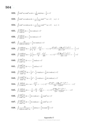
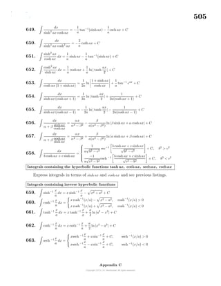
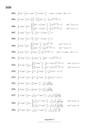
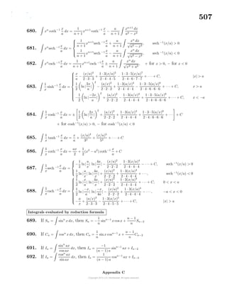
![509
703.
J1(x)
x
dx = −J1(x) + J0(x) dx
704. xν
Jν−1(x) dx = xν
Jν(x) + C
705. x−ν
Jν+1(x) dx = x−ν
Jν(x) + C
706.
J1(x)
xn
dx =
−1
n
J1(x)
xn−1
+
1
n
J0(x)
xn−1
dx
707. xJ0(x) dx = xJ1(x) + C
708. x2
J0(x) dx = x2
J1(x) + xJ0(x) − J0(x) dx
709. xn
J0(x) dx = xn
J1(x) + (n − 1)xn−1
J0(x) − (n − 1)2
xn−2
J0(x) dx
710.
J0(x)
xn
dx =
J1(x)
(n − 1)2xn−2
−
J0(x)
(n − 1)xn−1
−
1
(n − 1)2
J0(x)
xn−2
dx
711. Jn+1(x) dx = Jn−1(x) dx − 2Jn(x)
712. xJn(αx)Jn(βx) dx =
x
β2 − α2
[αJn(αx)Jn(βx) − βJn(βx)Jn(αx)] + C
713. If Im,n = xm
Jn(x) dx, m ≥ −n, then
Im,n = −xm
Jn−1(x) + (m + n − 1) Im−1,n−1
714. If In,0 = xn
J0(x) dx, then In,0 = xn
J1(x) + (n − 1)xn−1
J0(x) − (n − 1)2
In−2,0 Note that
I1,0 = xJ0(x) dx = xJ1(x) + C and I0,1 = J1(x) dx = −J0(x) + C Note also that the integral
I0,0 = J0(x) dx cannot be given in closed form.
Appendix C](https://image.slidesharecdn.com/calculusvolume-1-160216221448/85/Calculus-volume-1-517-320.jpg)
![510
Definite integrals
General integration properties
1. If
dF (x)
dx
= f(x), then
b
a
f(x) dx = F (x)|
b
a = F (b) − F (a)
2.
∞
0
f(x) dx = lim
b→∞
b
0
f(x) dx,
∞
−∞
f(x) dx = lim
b→∞
a→−∞
b
a
f(x) dx
3. If f(x) has a singular point at x = b, then
b
a
f(x) dx = lim
→0
b−
a
f(x) dx
4. If f(x) has a singular point at x = a, then
b
a
f(x) dx = lim
→0
b
a+
f(x) dx
5. If f(x) has a singular point at x = c, a < c < b, then
b
a
f(x) dx =
c−
a
f(x) dx +
b
c+
f(x) dx
6.
b
a
cf(x) dx =c
b
a
f(x) dx, c constant
a
a
f(x) dx =0,
b
0
f(x) dx =
b
0
f(b − x) dx
b
a
f(x) dx = −
a
b
f(x) dx,
b
a
f(x) dx =
c
a
f(x) dx +
b
c
f(x) dx
7. Mean value theorems
b
a
f(x) dx =f(c)(b − a), a ≤ c ≤ b
b
a
f(x)g(x) dx =f(c)
b
a
g(x) dx, g(x) ≥ 0, a ≤ c ≤ b
b
a
f(x)g(x) dx = f(a)
ξ
a
g(x) dx
b
a
f(x)g(x) dx = f(b)
b
η
g(x) dx
a < ξ < b a < η < b
The last mean value theorem requires that f(x) be monotone increasing and nonnegative
throughout the interval (a, b)
8. Numerical integration
Divide the interval (a, b) into n equal parts by defining a step size h = b−a
n .
Two numerical integration schemes are
(a) Trapezoidal rule with global error −(b−a)
12
h2
f (ξ) for a < ξ < b.
b
a
f(x) dx =
h
2
[f(x0) + 2f(x1) + 2f(x2) + · · ·2f(xn−1) + f(xn)]
(b) Simpson’s 1/3 rule with global error −(b−a)
90
h4
f(iv)
(ξ) for a < ξ < b.
b
a
f(x) dx =
2h
3
[f(x0) + 4f(x1) + 2f(x2) + 4f(x3) + 2f(x4) + · · · + 2f(xn−2) + 4f(xn−1) + f(xn)]
Appendix C](https://image.slidesharecdn.com/calculusvolume-1-160216221448/85/Calculus-volume-1-518-320.jpg)
![513
42.
π
0
sinpθ sin qθ dθ =
0, p = q
π
2
, p = q
43.
π
0
sinpθ cos qθ dθ =
0, p + q even
2p
p2 − q2
, p + q odd
44.
π
0
x dx
a2 − cos2 x
=
π2
2a
√
a2 − 1
45.
π
0
dx
a + b cos x
=
π
√
a2 − b2
46.
π
0
sin θ dθ
1 − 2a cos θ + a2
=
2
a
tanh−1
a
47.
π
0
sin 2θ dθ
1 − 2a cos θ + a2
=
2
a2
(1 + a2
) tanh−1
a −
2
a
48.
π
0
x sinx dx
1 − 2a cos x + a2
=
π
a
ln(1 + a), |a| < 1
π ln 1 +
1
a
, |a| > 1
49.
π
0
cos pθ dθ
1 − 2a cos θ + a2
=
πap
1 − a2
, a2
< 1
πa−p
a2 − 1
, a2
> 1
50.
π
0
cos pθ dθ
(1 − 2a cos θ + a2)2
=
πap
(1 − a2)3
[(p + 1) − (p − 1)a2
], a2
< 1
πa−p
(a2 − 1)3
[(1 − p) + (1 + p)a2
], a2
> 1
51.
π
0
cos pθ dθ
(1 − 2a cos θ + a2)3
=
πap
2(1 − a2)5
(p + 2)(p + 1) + 2(p + 2)(p − 2)a2
+ (p − 2)(p − 1)a4
, a2
< 1
πa−p
2(a2 − 1)5
(1 − p)(2 − p) + 2(2 − p)(2 + p)a2
+ (2 + p)(1 + p)a4
, a2
> 1
52.
2π
0
dx
(a + b sinx)2
=
2πa
(a2 − b2)3/2
53.
2π
0
dx
a + b sinx
=
2π
√
a2 − b2
54.
2π
0
dx
a + b cos x
=
2π
√
a2 − b2
55.
2π
0
dx
(a + b sinx)2
=
2πa
(a2 − b2)3/2
56.
2π
0
dx
(a + b cos x)2
=
2πa
(a2 − b2)3/2
57.
L
−L
sin
mπx
L
sin
nπx
L
dx =
0, m = n, m, n integers
L
2
, m = n
Appendix C](https://image.slidesharecdn.com/calculusvolume-1-160216221448/85/Calculus-volume-1-521-320.jpg)
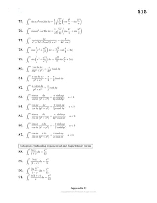
![518
127.
∞
0
x4
e−x2
cos ax dx =
√
π
8
3 − 3a2
+
a4
4
e−a2
/4
128.
∞
0
ln x
x − 1
3
dx = π2
129.
∞
−∞
x sin rx dx
(x − b)2 + a2
=
π
a
(a cos br + b sin br) e−ar
130.
∞
−∞
sin rx dx
x[(x − b)2 + a2]
=
π
a(a2 + b2)
a − (cos br − b sin br) e−ar
131.
∞
−∞
cos rx dx
(x − b)2 + a2
=
π
a
e−ar
cos br
132.
∞
−∞
sin rx dx
(x − b)2 + a2
=
π
a
e−ar
sin br
133.
∞
−∞
e−x2
cos 2nx dx =
√
π e−n2
134.
∞
0
xp−1
ln x
1 + x
dx =
−π2
sin pπ
cot pπ, 0 < p < 1
135.
∞
0
e−x
ln x dx = −γ
136.
∞
0
e−x2
ln x dx = −
√
π
4
(γ + 2 ln2)
137.
∞
0
ln
ex
+ 1
ex − 1
dx =
π2
4
138.
∞
0
x dx
ex − 1
=
π2
6
139.
∞
0
x dx
ex + 1
=
π2
12
Integrals containing hyperbolic terms
140.
1
0
sinh(m ln x)
sinh(ln x)
dx =
π
2
tan
mπ
2
, |m| < 1
141.
∞
0
sin ax
sinh bx
dx =
π
2b
tanh(
πa
2b
)
142.
∞
0
cos ax
cosh bx
dx =
π
2b
sech (
πa
2b
)
143.
∞
0
x dx
sinh ax
=
π2
4a2
Appendix C](https://image.slidesharecdn.com/calculusvolume-1-160216221448/85/Calculus-volume-1-526-320.jpg)
![519
144.
∞
0
sinh px
sinh qx
dx =
π
2q
tan(
πp
2q
), |p| < q
145.
∞
0
cosh ax − cosh bx
sinh πx
dx = ln
cos b
2
cos a
2
, −π < b < a < π
146.
∞
0
sinh px
sinh qx
cos mx dx =
π
2q
sin πp
q
cos πp
q
+ cosh πm
q
, q > 0, p2
< q2
147.
∞
0
sinh px
cosh qx
sin mx dx =
π
q
sin pπ
2q
sinh mπ
2q
cos pπ
q + cosh mπ
q
148.
∞
0
cosh px
cosh qx
cos mx dx =
π
q
cos pπ
2q cosh mπ
2q
cos pπ
q + cosh mπ
q
Miscellaneous Integrals
149.
x
0
ξλ−1
[1 − ξµ
]ν
dξ =
xλ
λ
F (−ν,
λ
µ
;
λ
µ
+ 1; xµ
) See hypergeometric function
150.
π
0
cos(nφ − x sin φ) dφ = π Jn(x)
151.
a
−a
(a + x)m−1
(a − x)n−1
dx = (2a)m+n−1 Γ(m)Γ(n)
Γ(m + n)
152. If f (x) is continuous and
∞
1
f(x) − f(∞)
x
dx converges, then
∞
0
f(ax) − f(bx)
x
dx = [f(0) − f(∞)] ln
b
a
153. If f(x) = f(−x) so that f(x) is an even function, then
∞
0
f x −
1
x
dx =
∞
0
f(x) dx
154. Elliptic integral of the first kind
θ
0
dθ
1 − k2 sin2
θ
= F (θ, k), 0 < k < 1
155. Elliptic integral of the second kind
θ
0
1 − k2 sin2
θ dθ = E(θ, k)
156. Elliptic integral of the third kind
θ
0
dθ
(1 + n sin2
θ) 1 − k2 sin2
θ
= Π(θ, k, n)
Appendix C](https://image.slidesharecdn.com/calculusvolume-1-160216221448/85/Calculus-volume-1-527-320.jpg)
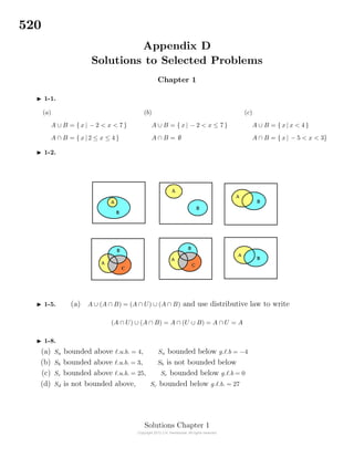
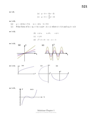
![526
Chapter 2
2-1. (b) y − 4 = 4(x − 2) (c) y − 4 = −4(x + 2)
2-2. (d)
dy
dx
= −
b + 2ax
(ax2 + bx + c)2
(h)
dy
dx
= 3(2x + 1)2
(2)(3x2
− x)2
+ (2x + 1)3
2(3x2
− x)(6x − 1)
which can also be expressed in the form
dy
dx
= 2x(3x − 1)(1 + 2x)2
(−1 + x + 21x2
)
2-3. (d)
dy
dx
=
−1
2x3/2
(j)
dy
dx
= 1 + ln x (l)
dy
dx
=
1
n
(a + x)
1
n −1
2-4. (b)
dy
dx
= −
√
x
(1 + x)2
+
1
2
√
x(1 + x)
(f)
dy
dx
=
x(3x2
− 2x)
2
√
x3 − x2
+ x3 − x2
(k)
dy
dx
=
−x
(1 + x2)3/2 1 − 1
1+x2
2-5. (g)
dy
dθ
= 6 cos(3θ) sin(3θ) = 3 sin(6θ)
(k)
dy
dx
= −
a − 2bx
1 − (ax − bx2)2
(l)
dy
dx
= xx
(1 + lnx) + x1/x 1
x2
−
ln x
x2
2-6. (j) y =
−2x
(1 + x2)2 1−x2
1+x2
(k) y =
(b + 2cx) sec[ln(a + bx + cx2
)] tan[ln(a + bx + cx2
)]
a + bx + cx2
2-7. (e) y =
−x
y2 − 2
(j) y =
3x2
− y + 6xy + 3y2
x − 3x2 − 6xy − 3y2
(l) y =
yxy−1
1 − x4 ln x
2-8. (d) y =
2x
√
1 − x4
(g) y =
1 + x
√
1 − x2
+sin−1
x (j) y = (cos(3x))x
(ln | cos 3x| − 3x tan(3x))
2-9. (d) y = (3 + x)x x
3 + x
+ ln(3 + x) (i) y = xx
(1 + ln x)
(l) y =
6x cos(4x) sin2
(4x)
sin3
(4x)
+ sin3
(4x)
2-10. (b) y =
−2ax
√
1 − a2x4
(h) y =
3
√
3x − 1
√
1 + 3x
=
3
√
9x2 − 1
(l) y =
3x2
√
1 − x6
Solutions Chapter 2](https://image.slidesharecdn.com/calculusvolume-1-160216221448/85/Calculus-volume-1-534-320.jpg)
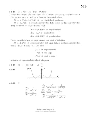
![533
Chapter 3
3-1. (a) 4
3
x3
+ 2x2
+ x + C or 1
6
(2x + 1)3
+ C1
(b) − csc(t) + C
(c) − 1
2
cos2
x + C1 or 1
2
sin2
x + C2
3-2. (a) 1
10 sin5
(2t) + sin4
(2t) + 4 sin3
(2t) + 8 sin2
(2t) + 8 sin(2t) + C1 or 1
10 [2 + sin(2t)]5
+ C2
(c) 4x2
4 ln 2
+ C
(e) − 1
3
cos(3x + 1) + C
3-3. (a) 1
3
tan(3x + 4) + C (c) 1
3
sec(3x + 4) + C (e) 1
6
ln| sin(3x2
)| + C
3-4. (a) 1
2
sin−1
(x2
) + C (c) −
√
1 − x2 (e) 1
2
sinh(x2
) + C
3-5. (a) − 1
3 sinh(3x+1)
+ C (c) − 1
3
coth(3x + 1) + C (e) 1
3
(3x + 1)2 − 1
3-6. (a) − 1
x + 5x + lnx + C (c) 2c
√
t + at + 2
3 bt3/2
+ C (e) 1
3b (a + bu2
)
√
a + bu2
3-7. (a) 26
3
Area under parabola
(b) 2 Area under sine curve
(c) 1
2
BH Area of triangle
3-8. (a) Let u = 3x + 1 = tan θ with du = 3 dx = sec2
θ dθ
then
1
3
csc θ dθ = −
1
3
ln| csc θ + cot θ| = −
1
3
ln
√
1 + u2
u
+
1
u
= −
1
3
ln |1 + 1 + u2| +
1
3
lnu + C where u = 3x + 1
3-9. Two functions with the same derivative differ by some constant value.
3-10. Use table III with appropriate scaling.
3-11. (a) ln|x − 3| + ln |x − 2| + ln|x − 1| + C
(c) tan−1
x + ln(x + 1) + ln(x2
+ 1) + C
(e) x +
3
2
x2
+ x3
+
1
2
x4
−
1
1 + x + x2
+ ln |x − 1| + C
Solutions Chapter 3](https://image.slidesharecdn.com/calculusvolume-1-160216221448/85/Calculus-volume-1-541-320.jpg)
![534
3-12. (a) dy = x dx
y
1
dy =
x
1
x dx =⇒ y − 3 =
1
2
(x2
− 1) or y =
1
2
x2
+
5
2
(c) dy = sin(3x) dx
y
1
dy =
1
3
x
0
sin(3x) 3dx =⇒ y − 1 =
1
3
[1 − cos(3x)]
or y =
4
3
−
1
3
cos(3x)
(e) dy = sin2
(3x) dx
y
1
dy =
1
3
x
0
sin2
(3x) 3 dx =⇒ y − 1 =
1
12
[6x − sin(6x)]
or y = 1 −
1
2
x −
1
12
sin(6x)
3-13. (b) x − tan−1
x + C (d) x −
1
x + 1
− 2 ln(x + 1) + C (f)
1
a
ln x −
1
a
ln(x − a) + C
3-14. (b)
1
(b − a)(x − a)
+
1
(a − b)2
[ln(x − b) − ln(x − a)] + C
(d)
ln(x2
− b2
)
2(b2 − a2)
+
ln(x − a)
a2 − b2
−
a
b(b2 − a2)
tan−1 x
b
+ C
(f)
−1
a2 + b2
1
b
tan−1 x
b
+
1
a
tan−1 x
b
+ C
3-15. (b) 1 (d)
1
4
+
e2
4
(f) 100
√
15
3-16. (b) (x2
−2x+2)ex
+C (d)
1
2
(sin x−cos x)ex
+C (f)
1
2
sec x tanx+
1
2
ln | secx+tan x|+C
3-17. (a)
eax
a2 + b2
(a sinbx − b cos bx)+C (c)
x
2
−
x2
4
−
1
2
ln(x+1)+
x2
2
ln(x+1)+C (e) e−2
3-18. (a)
1
0
f(x) dx
3-19. A =
5
−1
[(4y − 1) − (y2
− 6)] dy, =⇒ A = 36
3-21. (a) Use symmetry to find
area ABH = area BCD =
4
0
( y + 4 − 4 − y) dy =
32
3
(
√
2 − 1)
3-23. (d) −
1
3
(a2
− x2
)3/2
+ C (e) 2x − 2x lnx + x(lnx)2
+ C (f)
x
a
−
1
a2
eax
+ C
3-24. (a) ln[t + 2 + t2 + 4t − 3] + C (d)
1
9
tan−1
x + C (e)
1
18
[ln(x − 1) − ln(x + 1)] + C
3-25. (a) 2 ln(1+
√
x)+C (f) −a b2 − (x + a)2+(b−a2
) tan−1 (a + x) b2 − (a + x)2
b2 − a2 − 2ax − x2
+C
Solutions Chapter 3](https://image.slidesharecdn.com/calculusvolume-1-160216221448/85/Calculus-volume-1-542-320.jpg)
![535
3-26. (c) 2
√
x − 2 ln(1 +
√
x) + C (f)
1
2
x − x2 + (2x − 1) sin−1
√
x + C
3-27. (c) (x2
+ 1) ex
(d) 1 − x2
5
8
x −
1
4
x2
+
3
8
sin−1
x + C
3-28. Surface S =
64
3
π and volume V = 5π2
3-29. (b) α = 1
3-32. (b)arc lengths = 16
3-35. (i) Surface area S =
28
√
2
3
π (ii) volume V = 12π
3-36. (i) Surface area S =
π
27
(145)3/2
− (10)3/2
(ii) Volume V =
762
7
π
3-37. (a)
2
π
(b)
2
π
(c)
4
3π
3-38. (d) 2 (f)
1
2
ln2
3-39. The area of three sides need to be calculated. Call these surface areas S1, S2
and S3. Show S = S1 + S2 + S3 = 11
√
2π + 9
√
2π + 20π
3-44. (a) A =
2π
0
r dθ (b) A = 2π
r
0
x dx (c) A =
2π
0
r
0
r drdθ
3-45. The figure illustrated in the problem 3-45, without the axes, is known as the
symbol the Pythagoreans use to represent their society.
(a) Divide area into four symmetric parts and show the area of one of these parts
is A1 = r2
0
π
6
−
√
3
8
and the total area is A = 4A1 = r2
0
2
3
π −
√
3
2
(b) Volume is given by V =
5
12
π r3
0
3-47. (a) 80 (b) 8 (c)
1
4
[ a2
c2
− b2
c2
− a2
d2
+ b2
d2
]
3-50. c = 1
2 (a + b)
Solutions Chapter 3](https://image.slidesharecdn.com/calculusvolume-1-160216221448/85/Calculus-volume-1-543-320.jpg)
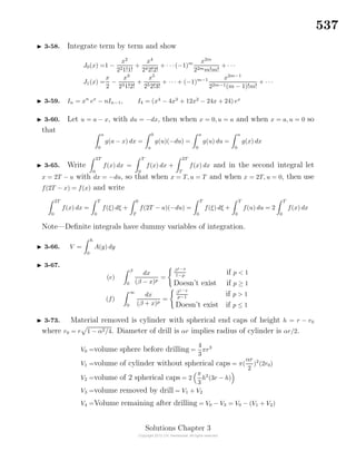
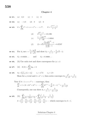
![539
4-10. (d) un =
n
(n + 1)(n + 2)(n + 3)
=
1/2
n + 1
−
1
n + 2
+
1/2
n + 3
so that the Nth partial
sum can be written
UN =
N
n=1
un =
5N + N2
12(6 + 5N + N2)
Divide numerator and denominator by N2
and show lim
N→∞
UN =
1
12
4-11. (d) If f(x) = 1
x ln x
, then T
M
f(x) dx =
T
M
1
x ln x
dx
Let u = lnx with du = 1
x dx and show T
M
f(x) dx = ln[ln x]T
M = ln[lnT] − ln[lnM]
Show this result increases without bound as T → ∞ so the integral diverges and
series diverges.
4-12. Let un =
1
np
, where
∞
n=1
1
np
is the p-series which converges p > 1 and diverges
p ≤ 1. Now select vn = np
f(n) and follow results for modification of a series.
4-13. (d) Since 3n2
+2n+1 > n2
, then
1
3n2 + 2n + 1
<
1
n2
and we know the p-series,
with p = 2 converges.
4-14. (iv)
4
n=1
(−1)n+1 1
n4
= 0.945939 with error E <
1
54
= 0.0016
8
n=1
(−1)n+1 1
n4
= 0.94694 with error E| <
1
94
= 0.000152416
4-15. (A) converges slower than (B)
4-17. xn = xn−1 −
x2
n − 3xn + 1
2xn − 3
x0 = 2, . . ., x4 = 2.61803
Exact roots are x =
3 ±
√
5
2
Convergence to desired root depends upon position
of initial guess.
4-18. Converges |x| < 1 and diverges for |x| > 1
4-20. Assume
∞
n=1
un converges by ratio test so that lim
n→∞
un+1
un
= p < 1. Let vn = 1
un
and examine
∞
n=1
vn using the ratio test to show series diverges.
Solutions Chapter 4](https://image.slidesharecdn.com/calculusvolume-1-160216221448/85/Calculus-volume-1-547-320.jpg)
![541
4-30. Use ratio test
4-33. Write (a+ b)r
= [a(1 + b/a)]r
= ar
(1 + b/a)r
and let x = b/a and then examine the
series f(x) = (1 + x)r
. Here
f (x) =r(1 + x)r−1
f (x) =r(r − 1)(1 + x)r−2
...
...
f(n)
(x) =r(r − 1)(r − 2) · · ·(r − (n − 1)(1 + x)r−n
This series has the power series expansion
f(x) = (1 + x)r
= 1 +
r
1
x +
r
2
x2
+
r
3
x3
+ · + Rn
Using the Lagrange form of the remainder
Rn =
xn
n!
f(n)
(θx) =
r
n
xn
(1 + θx)r−n
where 0 < θ < 1. For 0 ≤ x < 1 and n > r, then one can show (1 + θx)r−n
< 1 and
r
n
xn
→ 0 as n → ∞ The Lagrange form for the remainder doesn’t aid in the analysis
of the region −1 < x ≤ 0 and so one can use the Cauchy form of the remainder to
analyze the remainder in this region.
The Cauchy form of the remainder is
Rn =
r(r − 1)(r − 2) · · ·(r − n + 1)
(n − 1)!
(1 − θ)n−1
xn
(
1 + θx)n−m
, 0 < θ < 1
If |x| < 1, then 1−θx
1+θx
< 1 so that
(1 − θ)n−1
(1 + θx)n−1 · 1
1+θx
1−m
<
1
(1 + θx)1−m
For −1 < x ≤ 0 the term 1
(1+θx)1−m = K is some constant independent of the index n
and the term
r(r − 1) · · ·(r − n + 1)
(n − 1)!
= r
(r − 1)!
(n − 1)!(r − n)!
= r
r − 1
n − 1
Therefore,
|Rn| < K|r|
r − 1
n − 1
|x|n
→ 0 as n → ∞
So the binomial series converges as |Rn| → 0 for |x| < 1
Solutions Chapter 4](https://image.slidesharecdn.com/calculusvolume-1-160216221448/85/Calculus-volume-1-549-320.jpg)
![542
4-36. y1 = α0 + 1
α1+ 1
x
= α0 + x
α1x+1 Here Q1 = α1x + 1 and
dy1
dx
=
(α1x + 1)(1) − x(α1)
(α1x + 1)2
=
1
[Q1(x)]2
4-41. For n, m integers and n = m
(sinnx, sin mx) =
π
0
sin nx sin mx dx =
sin[(m − n)x]
2(m − n)
−
sin[(m + n)x]
2(m + n)
π
0
= 0, m = n
sin nx 2
= (sinnx, sinnx) =
π
0
sin2
(nx) dx =
x
2
−
sin 2nx
4n
π
0
=
π
2
or sinnx =
π
2
. The set of functions
2
π
sin nx is therefore an orthonormal set
with norm-squared equal to unity.
4-42. (c)
(1, cos
nπx
L
) =
L
−L
cos
nπx
L
dx = 0
(1, sin
nπx
L
) =
L
−L
sin
nπx
L
dx = 0
(cos
nπx
L
, cos
mπx
L
) =
L
−L
cos
nπx
L
sin
mπx
L
dx = 0, m = n
(cos
nπx
L
, cos
mπx
L
) =
L
−L
cos
nπx
L
cos
mπx
L
dx = 0
(sin
nπx
L
, sin
mπx
L
) =
L
−L
sin
nπx
L
sin
mπx
L
dx = 0 m = n
(1, 1) = 1 2
= 2L
(sin
nπx
L
, sin
nπx
L
) = sin
nπx
L
2
= L
(cos
nπx
L
, cos
nπx
L
) = cos
nπx
L
2
= L
4-43. (e) (i) If f(x) is even, bn = 0 and a0 =
1
L
L
0
f(x) dx, an =
2
L
L
0
f(x) cos
nπx
L
dx
(ii) If f(x) is odd, a0 = an = 0 and bn =
2
L
L
0
f(x) sin
nπx
L
dx
Solutions Chapter 4](https://image.slidesharecdn.com/calculusvolume-1-160216221448/85/Calculus-volume-1-550-320.jpg)
![543
4-44. Roots are (2, 3) and (−1, 1)
4-48. (a) C =
C0e−kτ
1 − e−kτ
(c) kτ = − ln
Cs
C0
− 1
Cs
C0
4-53. y = sin x + y =⇒ y2
= sinx + y Differentiate this relation to obtain given
answer.
4-55. If ex cos x
= a0 + a1x + a2x2
+ a3x3
+ · · ·, then its derivative is
ex cos x
[cos x − x sinx] = a1 + 2a2x + 3a3x2
+ 4a4x3
+ · · ·
Show
cos x − x sin x = 1 −
3
2
x2
+
5
24
x4
−
7
720
x6
+
1
4480
x8
+ · · ·
and substitute the top line equation and third line equation into the second line
equation to obtain
(a0 + a1x + a2x2
+ · · ·)(1 −
3
2
x2
+
5
24
x4
+ · · ·) = a1 + 2a2x + 3a3x2
+ · · ·
Expanding the left-hand side of this equation gives
a0 + a1x + (a2 −
3
2
a0)x2
+ (a3 −
3
2
a1)x3
+ · · · = a1 + 2a2x + 3a3x2
+ · · ·
Equate like powers of x to find a relation between the coefficients. Use top line
equation to show at x = 0 that a0 = 1 and from equating like powers of x one finds
a1 = 1, a2 = 1/2, a3 = −1/3, a4 = −11/24, etc
Solutions Chapter 4](https://image.slidesharecdn.com/calculusvolume-1-160216221448/85/Calculus-volume-1-551-320.jpg)
![544
Chapter 5
5-1. V =
4
3
πr3
,
dV
dt
= 4πr2 dr
dt
, α = 4πr2
0
dr
dt
=⇒
dr
dt
=
α
4πr2
0
5-2. pv1.4
= c,
dp
dt
v1.4
+ p(1.4)v0.4 dv
dt
= 0 or
dp
dt
= −1.4
p
v
dv
dt
(a) dp
dt
= −1.4p
v
α
(b) dv
dt
= β
1.4
v
p
5-3.
+ s
10
=
s
5.5
, if d
dt
= 4 ft/s, then show
ds
dt
=
22
4.5
ft/s.
5-4. (a) Let S1 = x − f > 0 and S2 = y − f > 0, then
1
x − f + f
+
1
y − f + f
=
1
f
or
1
S1 + f
+
1
S2 + f
=
1
f
Simplify this expression and show f2
= S1S2
(b) Differentiate the lens law and show
dy
dt
= −
y2
x2
r0
5-5. Area of equilateral triangle with side x is A =
√
3
8
x2
so that
dA
dt
=
2
√
3
8
x
dx
dt
Now substitute x = x0 and dx
dt
= r0
5-6. p = p0e−α0h
(a) [p0] = lbs/ft2
, [α0] = 1/ft
(b)
dh
dt
= 10 ft/s
dp
dt
= p0e−α0h
(−α0
dh
dt
) Substitute for dh
dt
and find the pressure
decreases with height.
5-7. y−y0 = α(x−x0)2
has the derivative
dy
dx
= 2α(x−x0). When x = ξ, the slope of the
tangent is m = 2α(ξ −x0) and the equation of the tangent line is y−η = 2α(ξ −x0)(x−ξ).
Here tan θ = m = 2α(ξ−x0) and if dξ
dt
= 1/2 cm/s, then sec2
θ
dθ
dt
= 2α
dξ
dt
or
dθ
dt
=
2α
1 + tan2
θ
dξ
dt
or
dθ
dt
=
2α
1 + 4α2(ξ − x0)2
1
2
5-8.
dT
dt
=
r0
c0
where c0 = V0/T0.
5-9.
dP
dt
= c0r0 where c0 = P0/T0.
Solutions Chapter 5](https://image.slidesharecdn.com/calculusvolume-1-160216221448/85/Calculus-volume-1-552-320.jpg)
![548
Integrate this equation and show
q = q0 cos
t
√
LC
and i =
dq
dt
= −
q0
√
LC
sin
t
√
LC
5-35. Hypothesis, y1 = y1(x) satisfies the given differential equation so that y +
P(x)y + Q(x)y = 0. If y2 = uy1 = u(x)y1(x), then by differentiation
y2 =uy1 + u y1
y2 =uy1 + 2u y1 + u y1
We desire to select u = u(x) such that y2 = y2(x) is also a function which satisfies the
differential equation. If y2 + P(x)y2 + Q(x)y2 = 0, the u = u(x) must be selected such
that
uy1 + 2u y1 + P(x)[uy1 + u y1] + Q(x)[uy1] = 0
Rearrange terms and show
y2 + P(x)y2 + Q(x)y2 = u [y1 + P(x)y1 + Q(x)y1]
zero by hypothesis
+u [2y1 + P(x)y1 + u y1 = 0
Therefore u = u(x) must be selected to satisfy
u [2y1 + P(x)y1] + u y1 = 0
Make the substitution u = v and u = dv
dx and show
v =
1
y2
1
e− P(x) dx
then another integration gives u.
5-36. (e) Integrate with respect to y and show
∂u
∂y
= xy +
y2
2
+ f(x), f(x) arbitrary function
Integrate again with respect to y holding x constant to obtain
u =
xy2
2
+
y3
6
+ yf(x) + g(x) where g(x) is another arbitrary function
(f) Integrate with respect to x and show
∂u
∂x
+ u = x + xy + f(y) f(y) arbitrary function
Solutions Chapter 5](https://image.slidesharecdn.com/calculusvolume-1-160216221448/85/Calculus-volume-1-556-320.jpg)
![549
Now multiply by ex
and show
∂u
∂x
ex
+ uex
=
∂
∂x
(uex
) = xex
+ xyex
+ f(y)ex
Integrate with respect to x and show
uex
= ex
(x − 1) + yex
(x − 1) + f(y)ex
+ g(y), g(y) arbitrary
5-37. (a) If ∂u
∂x
= ∂v
∂y
and ∂u
∂y
= −∂v
∂x
, then differentiate the first equation with respect
to x and differentiate the second equation with respect to y and show
∂2
u
∂x2
=
∂2
v
∂y ∂x
and
∂2
u
∂y2
= −
∂2
v
∂x ∂y
then by addition of these equations one obtains
∂2
u
∂x2
+
∂2
u
∂y2
= 0.
5-38.
Area= A = (2x)(2y) = 4xy = 4x
√
r2 − x2 since x2
+ y2
= r2
dA
dx
=
−4x2
√
r2 − x2
+ 4 r2 − x2
Show the derivative is zero when x = r/
√
2 and y = r/
√
2 and a
square is the maximum inscribed rectangle. To show it is a maxi-
mum examine dA
dx
for x < r/
√
2 and dA
dx
for x > r/
√
2
5-39. y = ex
for 0 ≤ x ≤ 1 use ds2
= dx2
+ dy2
and write ds = 1 + dy
dx
2
dx so
that s =
1
0
1 + e2x dx To evaluate this integral make the substitution u = ex
with
du = ex
dx and show s =
e
1
1 + u2
du
u
Make another substitution w2
= 1 + u2
with
2w dw = 2u du and show
s =
√
1+e2
√
2
w ·
w dw
√
w2 − 1
1
√
w2 − 1
s =
√
1+e2
√
2
w2
− 1 + 1
w2 − 1
dw
s =
√
1+e2
√
2
dw −
dw
1 − w2
= w]
√
1+e2
√
2
− tanh−1
w
√
1+e2
√
2
s = 1 + e2 −
√
2 + tanh−1
√
2 − tanh−1
( 1 + e2)
5-40. The side area is As = 2πrh and the ends (top and bottom) have area Ae = 2πr2
where πr2
h = πV0 is to be satisfied. The cost of construction is
C = c0 (2πrh) + 3c0 2πr2
Substitute into this equation h = V0
r2 to express C = C(r) as a function of r. Show
dC
dr
= 0 when r = 3
√
V 0/6 and h = 62/3 3
√
V 0. Show curve for C = C(r) is concave up at
this point and hence a minimum is achieved.
Solutions Chapter 5](https://image.slidesharecdn.com/calculusvolume-1-160216221448/85/Calculus-volume-1-557-320.jpg)
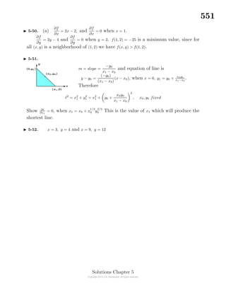
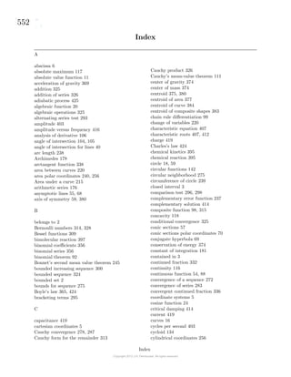


![[Deck] What's New in Spark-Iceberg Integration via DSV2.pptx](https://cdn.slidesharecdn.com/ss_thumbnails/deckwhatsnewinspark-icebergintegrationviadsv2-260210005337-25955b12-thumbnail.jpg?width=640&height=640&fit=bounds)


