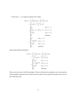
The document describes the DeBoor-Cox calculation, which relates the analytical and geometric definitions of B-spline curves. It begins by defining a B-spline curve analytically as a weighted sum of normalized B-spline blending functions and control points. The blending functions are defined recursively. DeBoor and Cox showed that starting from this analytical definition, one can derive the geometric definition of a B-spline curve as a pyramid of control points. Their calculation demonstrated the relationship between the two common definitions of B-splines.

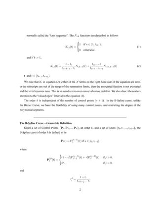

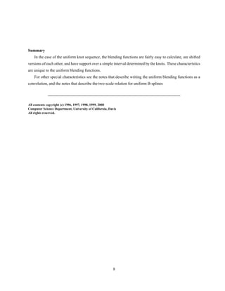
![If k = 2 then N0,2 can be written as a weighted sum of N0,1 and N1,1 by equation (2). This gives
N0,2(t) =
t − t0
t1 − t0
N0,1(t) +
t2 − t
t2 − t1
N1,1(t)
= tN0,1(t) + (2 − t)N1,1(t)
=
t if 0 ≤ t 1
2 − t if 1 ≤ t 2
0 otherwise
This curve is shown in the following figure. The curve is piecewise linear, with support in the interval [0, 2].
¡ ¢ £ ¤
¥§¦©¨
These functions are commonly referred to as “hat” functions and are used as blending functions in many
linear interpolation problems.
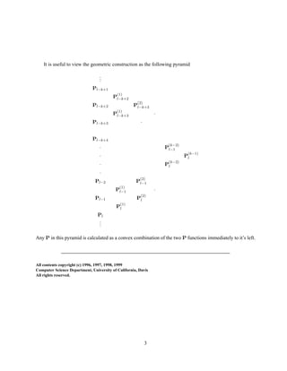
Similarly, we can calculate N1,2 to be
N1,2(t) =
t − t1
t2 − t1
N1,1(t) +
t3 − t
t3 − t2
N2,1(t)
= (t − 1)N1,1(t) + (3 − t)N2,1(t)
=
t − 1 if 1 ≤ t 2
3 − t if 2 ≤ t 3
0 otherwise
This curve is shown in the following figure, and it is easily seen to be a shifted version of N0,2.
4](https://image.slidesharecdn.com/b-spline-150510100035-lva1-app6892/85/B-spline-7-320.jpg)
![¡ ¢ £ ¤
¥§¦©¨
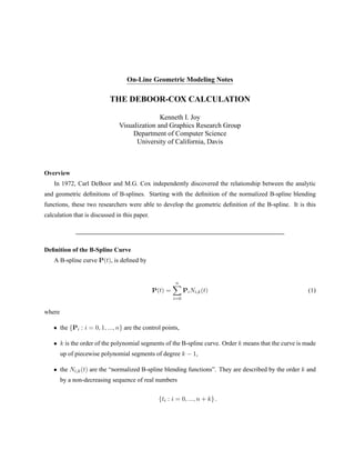
Finally, we have that
N1,2(t) =
t − 2 if 2 ≤ t 3
4 − t if 3 ≤ t 4
0 otherwise
which is shown in the following illustration.
¡ ¢ £ ¤
¥§¦©¨
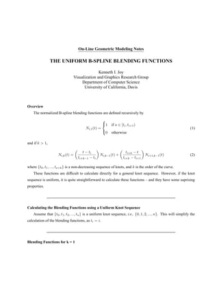
These nonzero portion of these curves each cover the intervals spanned by three knots – e.g., N1,2 spans the
interval [1, 3]. The curves are piecewise linear, made up of two linear segments joined continuously.
Sinve the curves are shifted versions of each other, we can write
Ni,2(t) = N0,2(t − i)
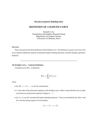
Blending Functions for k = 3
5](https://image.slidesharecdn.com/b-spline-150510100035-lva1-app6892/85/B-spline-8-320.jpg)
![¡ ¢ £ ¤
¥§¦©¨
!
§#©$%'(
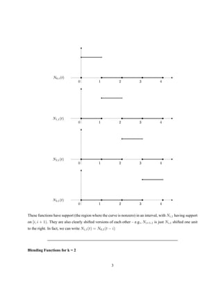
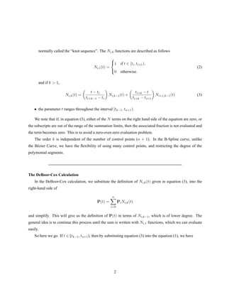
The nonzero portion of these two curves each span the interval between four consecutive knots – e.g., the
nonzero portion of N1,3 spans the interval [1, 4]. Again, N1,3 can be seen visually to be a shifted version of
N0,3. (This fact can also be seen analytically by substituting t + 1 for t in the equation for N1,3.) We can
write
Ni,3(t) = N0,3(t − i)
Blending Functions of Higher Orders
It is not too difficult to conclude that the Ni,4 blending functions will be piecewise cubic functions. The
support of Ni,4 will be the interval [i, i + 4] and each of the blending functions will be shifted versions of
each other, allowing us to write
Ni,4(t) = N0,4(t − i)
In general, the uniform blending functions Ni,k will be piecewise k − 1st degree functions having support
in the interval [i, i + k). They will be shifted versions of each other and each can be written in terms of a
“basic” function
Ni,k(t) = N0,k(t − i)
7](https://image.slidesharecdn.com/b-spline-150510100035-lva1-app6892/85/B-spline-10-320.jpg)
![P(t) =
n
i=0
PiNi,k(t)
=
n
i=0
Pi
t − ti
ti+k−1 − ti
Ni,k−1(t) +
ti+k − t
ti+k − ti+1
Ni+1,k−1(t)
Distributing the sums, we obtain
=
n
i=0
Pi
t − ti
ti+k−1 − ti
Ni,k−1(t) +
n
i=0
Pi
ti+k − t
ti+k − ti+1
Ni+1,k−1(t)
We now separate out those unique terms of each sum, N0,k−1 and Nn+1,k−1, giving
= P0
t − t0
tk−1 − t0
N0,k−1(t) +
n
i=1
Pi
t − ti
ti+k−1 − ti
Ni,k−1(t)
+
n−1
i=0
Pi
ti+k − t
ti+k − ti+1
Ni+1,k−1(t) + Pn
tn+k − t
tn+k − tn+1
Nn+1,k−1(t)
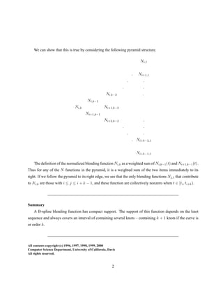
Now since the support of a B-spline blending function Ni,k(t) is the interval [ti, ti+k], we have that
N0,k−1 is non-zero only if t ∈ [t0, tk−1), which is outside the interval [tk−1, tn+1) (where P(t) is defined).
Thus, N0,k−1(t) ≡ 0. Also Nn+1,k−1 is non-zero only if t ∈ [tn+1, tn+k−1), which is outside the interval
3](https://image.slidesharecdn.com/b-spline-150510100035-lva1-app6892/85/B-spline-14-320.jpg)
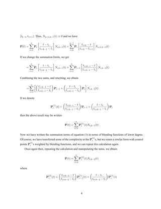
![(Note the appearance of the 2s on the right-hand side of the equation.)
If we continue with this process again, we will manipulate the sum so that the blending functions have
order k − 3. Then again with give us k − 4, and eventually we will obtain blending functions of order 1. We
are lead to the following result: If we define
P
(j)
i (t) =
(1 − τj
i )P
(j−1)
i−1 (t) + τj
i P
(j−1)
i (t) if j 0
Pi if j = 0
(4)
where
τj
i =
t − ti
ti+k−j − ti
Then, if t is in the interval [tl, tl+1), we have
P(t) = P
(k−1)
l (t)
This can be shown by continuing the DeBoor-Cox calculation k − 1 times. When complete, we arrive
at the formula
P(t) =
n
i=k−1
P
(k−1)
i (t)Ni,1(t)
where P
(j)
i (t) is given in equation (4). (Note the algebraic simplification that the τ’s provide.) If t ∈
[tl, tl+1], then then the only nonzero term of the sum is the lth term, which is one, and the sum must equal
P
(k−1)
l (t).
This enables us to define the geometrical definition of the B-spline curve.
Geometric Definition of the B-Spline Curve
Given a set of Control Points
P0, P1, ..., Pn
5](https://image.slidesharecdn.com/b-spline-150510100035-lva1-app6892/85/B-spline-16-320.jpg)