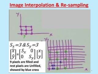
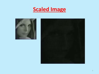
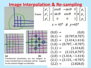
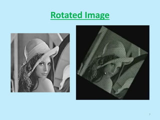
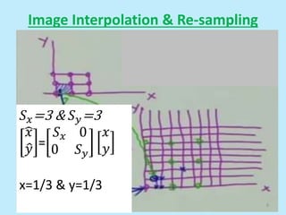
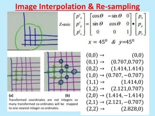
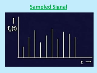
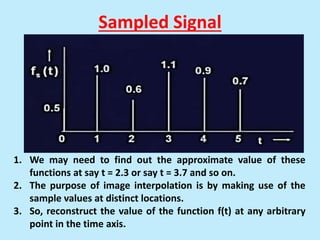
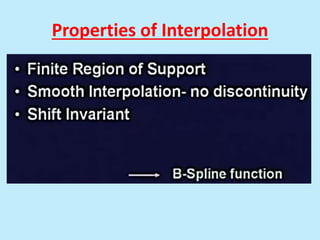
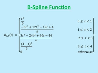
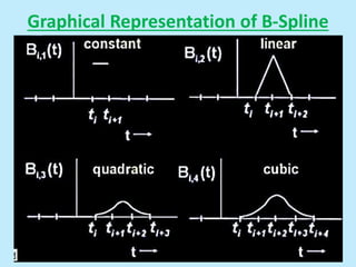
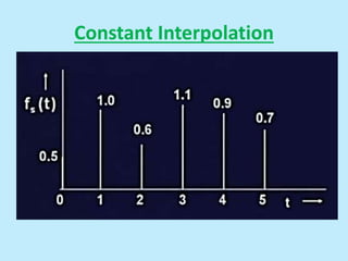
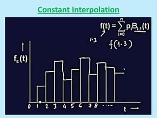
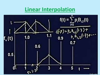
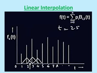
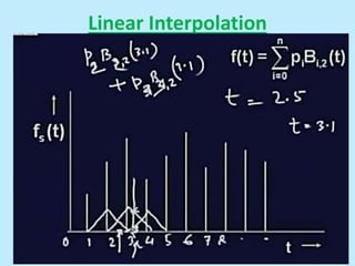
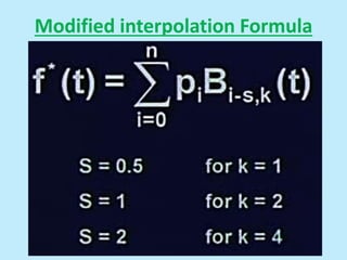
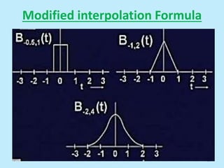
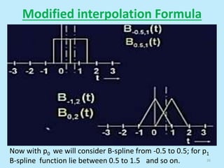
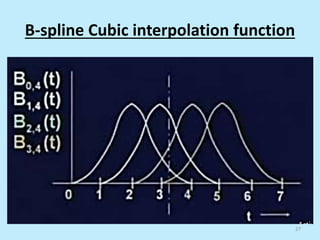
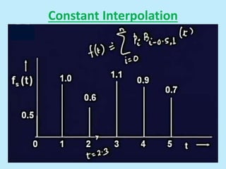
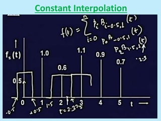
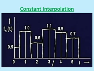
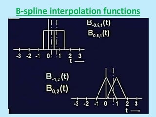
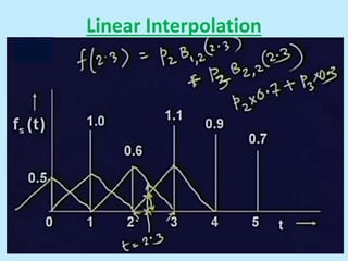
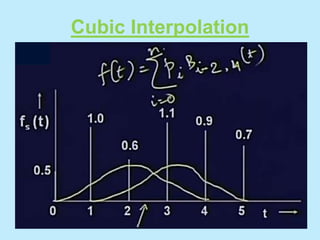
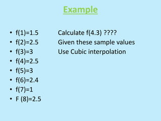
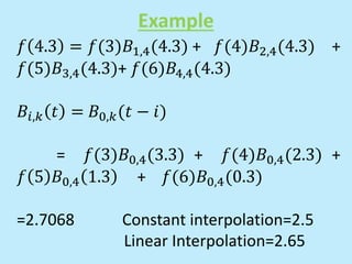
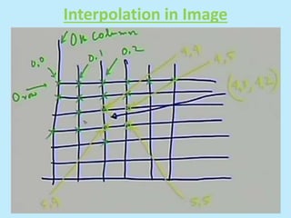
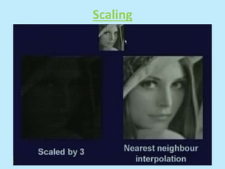
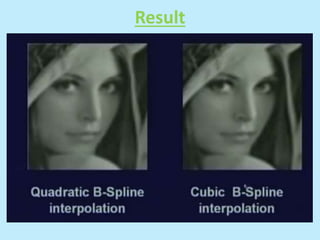
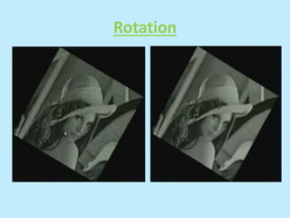
Digital Image
Processing
Dr. Rajib Kumar Jha
Associate Professor
Depart of Electrical Engineering
Indian Institute of Technology Patna
jharajib@iitp.ac.in
Lecture
Notes-2021
1
Lecture-7-8
Interpolation & Re-sampling
2
Contents
• Interpolation Operations
• When interpolation operations are needed
• B-Spline interpolations
3
Image Interpolation & Re-sampling
4
𝑆𝑥=3 & 𝑆𝑦=3
𝑥
𝑦 =
𝑆𝑥 0
0 𝑆𝑦
𝑥
𝑦
9 pixels are filled and
rest pixels are Unfilled,
showed by blue cross
Scaled Image
5
Image Interpolation & Re-sampling
(a) (b)
Transformed coordinates are not integers so
many transformed co-ordinates will be mapped
to one nearest integer co-ordinates.
𝑥 = 450
& y=450
0,0 → (0,0)
0,1 → (0.707,0.707)
0,2 → (1.414,1.414)
(1,0) → (0.707, −0.707)
1,1 → (1.414,0)
1,2 → (2.121,0.707)
(2,0) → (1.414, −1.414)
(2,1) → (2.121, −0.707)
2,2 → (2.828,0)
Rotated Image
7
Image Interpolation & Re-sampling
8
𝑆𝑥=3 & 𝑆𝑦=3
𝑥
𝑦 =
𝑆𝑥 0
0 𝑆𝑦
𝑥
𝑦
x=1/3 & y=1/3
Image Interpolation & Re-sampling
(a) (b)
Transformed coordinates are not integers so
many transformed co-ordinates will be mapped
to one nearest integer co-ordinates.
𝑥 = 450
& y=450
0,0 → (0,0)
0,1 → (0.707,0.707)
0,2 → (1.414,1.414)
(1,0) → (0.707, −0.707)
1,1 → (1.414,0)
1,2 → (2.121,0.707)
(2,0) → (1.414, −1.414)
(2,1) → (2.121, −0.707)
2,2 → (2.828,0)
Sampled Signal
Sampled Signal
1. We may need to find out the approximate value of these
functions at say t = 2.3 or say t = 3.7 and so on.
2. The purpose of image interpolation is by making use of the
sample values at distinct locations.
3. So, reconstruct the value of the function f(t) at any arbitrary
point in the time axis.
Properties of Interpolation
Properties
• I want to approximate the function value at locations
say t = 2.3, then the samples that should be
considered are the samples which are nearer to t =
2.3. We should not consider sample value at t = 50.
• we should not introduce any discontinuity in the
signal.
• Interpolation must be shift invariant. That is if we
shift the signal by say t = 5, even then the same
interpolation operation should give us the same
result in the same interval.
B-Spline Function
• B-Spline function is a piece wise polynomial
function that can be used to provide local
approximation of curves using very small number
of parameters.
• Because it is useful for local approximation of
curves so it can be very useful for smoothening
operation of some discrete curves,
• It is also very-very useful for interpolation of a
function from discrete number of samples.
B-Spline Function
15
So, this control points actually decide that how the B-spline
functions should be guided to give us a smooth curve.
Normalized B spline is Bi,k
of order k can be
recursively defined.
Pi is called control point
t
t
t
t
t
t
t
t
t
t t
t
t
t
B-Spline Function
𝐵0,1 t =
1 0 ≤ 𝑡 < 1
0 𝑜𝑡ℎ𝑒𝑟𝑤𝑖𝑠𝑒
𝐵0,2 t =
𝑡 0 ≤ 𝑡 < 1
2 − 𝑡 1 ≤ 𝑡 < 2
0 𝑜𝑡ℎ𝑒𝑟𝑤𝑖𝑠𝑒
𝐵0,3 t =
𝑡2
2
0 ≤ 𝑡 < 1
−𝑡2
+ 3𝑡 − 1.5 1 ≤ 𝑡 < 2
(3−𝑡)2
2
2 ≤ 𝑡 < 3
0 𝑜𝑡ℎ𝑒𝑟𝑤𝑖𝑠𝑒
B-Spline Function
𝐵0,4 t =
𝑡3
6
0 ≤ 𝑡 < 1
−3𝑡3 + 12𝑡2 − 12𝑡 + 4
6
1 ≤ 𝑡 < 2
3𝑡3
− 24𝑡2
+ 60𝑡 − 44
6
2 ≤ 𝑡 < 3
(4 − 𝑡)3
6
3 ≤ 𝑡 < 4
0 𝑜𝑡ℎ𝑒𝑟𝑤𝑖𝑠𝑒
Graphical Representation of B-Spline
Constant Interpolation
Linear Interpolation
21
Linear Interpolation
22
Linear Interpolation
Modified interpolation Formula
25
Modified interpolation Formula
26
Now with p0 we will consider B-spline from -0.5 to 0.5; for p1
B-spline function lie between 0.5 to 1.5 and so on.
B-spline Cubic interpolation function
27
Constant Interpolation
B-spline interpolation functions
Linear Interpolation
Cubic Interpolation
Example
• f(1)=1.5 Calculate f(4.3) ????
• f(2)=2.5 Given these sample values
• f(3)=3 Use Cubic interpolation
• f(4)=2.5
• f(5)=3
• f(6)=2.4
• f(7)=1
• F (8)=2.5
Example
𝑓 4.3 = 𝑓(3)𝐵1,4(4.3) + 𝑓(4)𝐵2,4(4.3) +
𝑓(5)𝐵3,4(4.3)+ 𝑓(6)𝐵4,4(4.3)
𝐵𝑖,𝑘 𝑡 = 𝐵0,𝑘(𝑡 − 𝑖)
= 𝑓(3)𝐵0,4(3.3) + 𝑓(4)𝐵0,4(2.3) +
𝑓 5 𝐵0,4 1.3 + 𝑓(6)𝐵0,4(0.3)
=2.7068 Constant interpolation=2.5
Linear Interpolation=2.65
Interpolation in Image
Scaling
Result
Rotation
Thanks
40
Contents
• Explain Image Transformation operations.
• Explain Unitary Transformations.
• Explain Orthogonal and Orthonormal basis vector.
• Explain how an arbitrary 1-D signal and
subsequently 2-D signal can be represented by
series summation of orthogonal basis vectors and
basis images.
• Computational Complexity of Image Transform
operation.
• Explain Separable Unitary Transformations.
By transformation getting an another image and by using
inverse transformation, get back the original image; then
why do we go for this transformation at all?
Image Transformations
The purpose of this image transformation operation is to
represent any arbitrary image as a series summation of such
unitary matrices or series summation of such basis images.
What is Unitary Transformation
• Discrete Fourier transform
coefficients or discrete cosine
transform coefficients, are different
types of unitary transformations.
Image Transformations
Let x (t) is an arbitrary signal which is a function of t.
Now signal x(t) can be represented as a series
summation of a set of unitary matrices or orthogonal
basis function.
Let {an (t)} is a set of real values
continuous fn.
𝑎𝑛 𝑡 = {𝑎0 𝑡 , 𝑎1 𝑡 , 𝑎𝑛 𝑡 ………}
Orthogonality condition is
0
𝑇
𝑎𝑚 𝑡 . 𝑎𝑛 𝑡 𝑑𝑡 =
𝑘 𝑖𝑓 𝑚 = 𝑛
0 𝑖𝑓 𝑚 ≠ 𝑛
X(t)
Image Transformation: An example
1. if I multiply sin(wt) with sin(3wt) and integrate, Similarly,
if I multiply sin(2wt) with sin(3wt) and integrate it will
be zero.
2. This particular set, sin(wt), sin(2wt), sin(3wt), is the set
of orthogonal basis functions.
Let x(t) is an arbitrary real values function.
This function x (t) can be represented by a series summation. So,
an (t) is the set of orthogonal basis functions.
by using that formula of orthogonality,
Properties of Basis function an(t)
an(t) is complete or closed if one of the two conditions hold.
1. There should be a signal x(t) having finite energy.
2. For any piecewise signal x(t), error energy should be
minimum.
• Let u(n) is a series of discrete samples represented in
the form of 1-D sequences. It has N samples
• For transformed vector v multiply u with
Transformation vector A. A is called unitary matrix of
size NxN
Discrete Sample Representation
u(n) : 0≤n≤ 𝑁 − 1
v = Au where
v is transformed vector and
A is Transformation vector
Unitary Matrix
53
u(n) is represented as the series summation of set
of basis vector. If it has the property of orthogonal
then above condition holds.
Now, the same concept of representing a vector as a
series summation of a set of basis vectors can also
be extended in case of an image.
Here {ak,l (m,n) } is called an image transform; is a
set of complete orthogonal discrete basis functions
satisfying two properties ORTHOGONALITY AND
COMPLETENESS
Properties of image transform an(t)
Previous Discussion
u(n) is one dimensional discrete signal. In
matrix representation
This transformation is unitary transformation if
Previous Discussion
The original image can be obtained as u=A-1v. This
expression says that the input sequence u (n) is now
represented in the form of series summation of a set of
vectors or orthonormal basis vectors.
Previous Discussion-2D
Set of Complete orthonormal basis function
Reduce the computational complexity (N4)
is separable if and only if
Separable Unitary Transform property
=
{
{
This is complete orthogonal basis vectors
How this Separable Unitary Transform
helps in reducing the complexity
A =B
A has NxN size; U has NxN size ; So, Order of AU is
O(N3 ); Order of A is O(N3 ); Order of V is 2*O(N3 )
DFT Basis Images
DCT Basis Images
Example: A is orthogonal matrix & U is
input image; V=AUAT
Transformed Image
What is Basis Images
Thanks
69

DIP_Lecture-35_36_RKJ_Interpolation_Resampling_Unitary_Transformations1.pptx

  • 1.
    Digital Image Processing Dr. RajibKumar Jha Associate Professor Depart of Electrical Engineering Indian Institute of Technology Patna jharajib@iitp.ac.in Lecture Notes-2021 1
  • 2.
  • 3.
    Contents • Interpolation Operations •When interpolation operations are needed • B-Spline interpolations 3
  • 4.
    Image Interpolation &Re-sampling 4 𝑆𝑥=3 & 𝑆𝑦=3 𝑥 𝑦 = 𝑆𝑥 0 0 𝑆𝑦 𝑥 𝑦 9 pixels are filled and rest pixels are Unfilled, showed by blue cross
  • 5.
  • 6.
    Image Interpolation &Re-sampling (a) (b) Transformed coordinates are not integers so many transformed co-ordinates will be mapped to one nearest integer co-ordinates. 𝑥 = 450 & y=450 0,0 → (0,0) 0,1 → (0.707,0.707) 0,2 → (1.414,1.414) (1,0) → (0.707, −0.707) 1,1 → (1.414,0) 1,2 → (2.121,0.707) (2,0) → (1.414, −1.414) (2,1) → (2.121, −0.707) 2,2 → (2.828,0)
  • 7.
  • 8.
    Image Interpolation &Re-sampling 8 𝑆𝑥=3 & 𝑆𝑦=3 𝑥 𝑦 = 𝑆𝑥 0 0 𝑆𝑦 𝑥 𝑦 x=1/3 & y=1/3
  • 9.
    Image Interpolation &Re-sampling (a) (b) Transformed coordinates are not integers so many transformed co-ordinates will be mapped to one nearest integer co-ordinates. 𝑥 = 450 & y=450 0,0 → (0,0) 0,1 → (0.707,0.707) 0,2 → (1.414,1.414) (1,0) → (0.707, −0.707) 1,1 → (1.414,0) 1,2 → (2.121,0.707) (2,0) → (1.414, −1.414) (2,1) → (2.121, −0.707) 2,2 → (2.828,0)
  • 10.
  • 11.
    Sampled Signal 1. Wemay need to find out the approximate value of these functions at say t = 2.3 or say t = 3.7 and so on. 2. The purpose of image interpolation is by making use of the sample values at distinct locations. 3. So, reconstruct the value of the function f(t) at any arbitrary point in the time axis.
  • 12.
  • 13.
    Properties • I wantto approximate the function value at locations say t = 2.3, then the samples that should be considered are the samples which are nearer to t = 2.3. We should not consider sample value at t = 50. • we should not introduce any discontinuity in the signal. • Interpolation must be shift invariant. That is if we shift the signal by say t = 5, even then the same interpolation operation should give us the same result in the same interval.
  • 14.
    B-Spline Function • B-Splinefunction is a piece wise polynomial function that can be used to provide local approximation of curves using very small number of parameters. • Because it is useful for local approximation of curves so it can be very useful for smoothening operation of some discrete curves, • It is also very-very useful for interpolation of a function from discrete number of samples.
  • 15.
    B-Spline Function 15 So, thiscontrol points actually decide that how the B-spline functions should be guided to give us a smooth curve. Normalized B spline is Bi,k of order k can be recursively defined. Pi is called control point t t t t t t t t t t t t t t
  • 16.
    B-Spline Function 𝐵0,1 t= 1 0 ≤ 𝑡 < 1 0 𝑜𝑡ℎ𝑒𝑟𝑤𝑖𝑠𝑒 𝐵0,2 t = 𝑡 0 ≤ 𝑡 < 1 2 − 𝑡 1 ≤ 𝑡 < 2 0 𝑜𝑡ℎ𝑒𝑟𝑤𝑖𝑠𝑒 𝐵0,3 t = 𝑡2 2 0 ≤ 𝑡 < 1 −𝑡2 + 3𝑡 − 1.5 1 ≤ 𝑡 < 2 (3−𝑡)2 2 2 ≤ 𝑡 < 3 0 𝑜𝑡ℎ𝑒𝑟𝑤𝑖𝑠𝑒
  • 17.
    B-Spline Function 𝐵0,4 t= 𝑡3 6 0 ≤ 𝑡 < 1 −3𝑡3 + 12𝑡2 − 12𝑡 + 4 6 1 ≤ 𝑡 < 2 3𝑡3 − 24𝑡2 + 60𝑡 − 44 6 2 ≤ 𝑡 < 3 (4 − 𝑡)3 6 3 ≤ 𝑡 < 4 0 𝑜𝑡ℎ𝑒𝑟𝑤𝑖𝑠𝑒
  • 18.
  • 19.
  • 20.
  • 21.
  • 22.
  • 23.
  • 24.
  • 25.
  • 26.
    Modified interpolation Formula 26 Nowwith p0 we will consider B-spline from -0.5 to 0.5; for p1 B-spline function lie between 0.5 to 1.5 and so on.
  • 27.
  • 28.
  • 29.
  • 30.
  • 31.
  • 32.
  • 33.
  • 34.
    Example • f(1)=1.5 Calculatef(4.3) ???? • f(2)=2.5 Given these sample values • f(3)=3 Use Cubic interpolation • f(4)=2.5 • f(5)=3 • f(6)=2.4 • f(7)=1 • F (8)=2.5
  • 35.
    Example 𝑓 4.3 =𝑓(3)𝐵1,4(4.3) + 𝑓(4)𝐵2,4(4.3) + 𝑓(5)𝐵3,4(4.3)+ 𝑓(6)𝐵4,4(4.3) 𝐵𝑖,𝑘 𝑡 = 𝐵0,𝑘(𝑡 − 𝑖) = 𝑓(3)𝐵0,4(3.3) + 𝑓(4)𝐵0,4(2.3) + 𝑓 5 𝐵0,4 1.3 + 𝑓(6)𝐵0,4(0.3) =2.7068 Constant interpolation=2.5 Linear Interpolation=2.65
  • 36.
  • 37.
  • 38.
  • 39.
  • 40.
  • 41.
    Contents • Explain ImageTransformation operations. • Explain Unitary Transformations. • Explain Orthogonal and Orthonormal basis vector. • Explain how an arbitrary 1-D signal and subsequently 2-D signal can be represented by series summation of orthogonal basis vectors and basis images. • Computational Complexity of Image Transform operation. • Explain Separable Unitary Transformations.
  • 42.
    By transformation gettingan another image and by using inverse transformation, get back the original image; then why do we go for this transformation at all?
  • 43.
  • 44.
    The purpose ofthis image transformation operation is to represent any arbitrary image as a series summation of such unitary matrices or series summation of such basis images.
  • 45.
    What is UnitaryTransformation • Discrete Fourier transform coefficients or discrete cosine transform coefficients, are different types of unitary transformations.
  • 46.
    Image Transformations Let x(t) is an arbitrary signal which is a function of t. Now signal x(t) can be represented as a series summation of a set of unitary matrices or orthogonal basis function. Let {an (t)} is a set of real values continuous fn. 𝑎𝑛 𝑡 = {𝑎0 𝑡 , 𝑎1 𝑡 , 𝑎𝑛 𝑡 ………} Orthogonality condition is 0 𝑇 𝑎𝑚 𝑡 . 𝑎𝑛 𝑡 𝑑𝑡 = 𝑘 𝑖𝑓 𝑚 = 𝑛 0 𝑖𝑓 𝑚 ≠ 𝑛 X(t)
  • 47.
    Image Transformation: Anexample 1. if I multiply sin(wt) with sin(3wt) and integrate, Similarly, if I multiply sin(2wt) with sin(3wt) and integrate it will be zero. 2. This particular set, sin(wt), sin(2wt), sin(3wt), is the set of orthogonal basis functions.
  • 48.
    Let x(t) isan arbitrary real values function. This function x (t) can be represented by a series summation. So, an (t) is the set of orthogonal basis functions.
  • 49.
    by using thatformula of orthogonality,
  • 50.
    Properties of Basisfunction an(t) an(t) is complete or closed if one of the two conditions hold. 1. There should be a signal x(t) having finite energy. 2. For any piecewise signal x(t), error energy should be minimum.
  • 51.
    • Let u(n)is a series of discrete samples represented in the form of 1-D sequences. It has N samples • For transformed vector v multiply u with Transformation vector A. A is called unitary matrix of size NxN Discrete Sample Representation u(n) : 0≤n≤ 𝑁 − 1 v = Au where v is transformed vector and A is Transformation vector
  • 52.
  • 53.
  • 55.
    u(n) is representedas the series summation of set of basis vector. If it has the property of orthogonal then above condition holds.
  • 56.
    Now, the sameconcept of representing a vector as a series summation of a set of basis vectors can also be extended in case of an image.
  • 57.
    Here {ak,l (m,n)} is called an image transform; is a set of complete orthogonal discrete basis functions satisfying two properties ORTHOGONALITY AND COMPLETENESS Properties of image transform an(t)
  • 59.
    Previous Discussion u(n) isone dimensional discrete signal. In matrix representation This transformation is unitary transformation if
  • 60.
    Previous Discussion The originalimage can be obtained as u=A-1v. This expression says that the input sequence u (n) is now represented in the form of series summation of a set of vectors or orthonormal basis vectors.
  • 61.
    Previous Discussion-2D Set ofComplete orthonormal basis function
  • 62.
    Reduce the computationalcomplexity (N4) is separable if and only if Separable Unitary Transform property = { { This is complete orthogonal basis vectors
  • 63.
    How this SeparableUnitary Transform helps in reducing the complexity A =B
  • 64.
    A has NxNsize; U has NxN size ; So, Order of AU is O(N3 ); Order of A is O(N3 ); Order of V is 2*O(N3 )
  • 65.
  • 66.
  • 67.
    Example: A isorthogonal matrix & U is input image; V=AUAT Transformed Image
  • 68.
  • 69.