resumen

1. CHAPTER 2
FOURIER ANALYSIS
The French mathematician J. B. J. Fourier (1758–1830) showed that arbitrary peri-
odic functions could be represented by an infinite series of sinusoids of harmonically
related frequencies. This was related to heat flow as the electrical applications were
not developed at that time. We first define periodic functions.
2.1 PERIODIC FUNCTIONS
A function is said to be periodic if it is defined for all real values of t and if there is a
positive number T such that
f(t) = f(t + T) = f(t + 2T) = f(t + nT) (2.1)
then T is called the period of the function.
If k is any integer and f(t + kT) = f(t) for all values of t and if two functions
f1(t) and f2(t) have the same period T, then the function f3(t) = af1(t) + bf2(t), where a
and b are constants, also has the same period T. Figure 2.1 shows periodic functions.
The functions
f1(t) = cos
2𝜋n
T
t = cos n𝜔0t
f2(t) = sin
2𝜋n
T
t = sin n𝜔0t (2.2)
are of special interest. Each frequency of the sinusoids n𝜔0 is said to be of nth har-
monic of the fundamental frequency 𝜔0, and each of these frequencies is related to
period t.
2.2 ORTHOGONAL FUNCTIONS
Two functions f1(t) and f2(t) are orthogonal over the interval (T1, T2) if
∫
T2
T1
f1(t) f2(t) = 0 (2.3)
Power System Harmonics and Passive Filter Designs, First Edition. J.C. Das.
© 2015 The Institute of Electrical and Electronics Engineers, Inc. Published 2015 by John Wiley & Sons, Inc.
31

2. 32 CHAPTER 2 FOURIER ANALYSIS
f(t)
–2T T
–T 0
T
0
T
0
2T
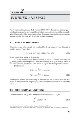
Figure 2.1 Periodic functions.
Figure 2.2 shows the orthogonal functions over a period T. Observe that
∫
T
0
sin m𝜔0t dt = 0 all m
∫
T
0
cos n𝜔0t dt = 0 all n ≠ 0 (2.4)
The average value of a sinusoid over m or n complete cycles is zero; therefore,
the following three cross products are also zero.
∫
T
0
sin m𝜔0tdt. cos n𝜔0tdt = 0 all m, n
∫
T
0
sin m𝜔0tdt. sin n𝜔0tdt = 0 m ≠ n
∫
T
0
cos m𝜔0tdt. cos n𝜔0tdt = 0 m ≠ n (2.5)

3. 2.3 FOURIER SERIES AND COEFFICIENTS 33
T/2 T/2
T/2
T T
T
T/2 T
f1(t)
f2(t)
f2(t)
f1(t)
Figure 2.2 Orthogonal functions.
Nonzero values occur when m = n:
∫
T
0
sin2
m𝜔0tdt = T∕2 all m
∫
T
0
cos2
m𝜔0tdt = T∕2 all n (2.6)
2.3 FOURIER SERIES AND COEFFICIENTS
A periodic function can be expanded in a Fourier series. The series has the expression:
f(t) = a0 +
∞
∑
n=1
(
an cos
(
2𝜋nt
T
)
+ bn sin
(
2𝜋nt
T
))
(2.7)
where a0 is the average value of function f(t). It is also called the DC component, and
an and bn are called the coefficients of the series. A series such as Eq. (2.7) is called
a trigonometric Fourier series. The Fourier series of a periodic function is the sum
of sinusoidal components of different frequencies. The term 2𝜋∕T can be written as
𝜔. The nth term n𝜔 is then called the nth harmonic and n = 1 gives the fundamental;
a0, an, and bn are calculated as follows:
a0 =
1
T ∫
T∕2
−T∕2
f(t)dt (2.8)
an =
2
T ∫
T∕2
−T∕2
cos
(
2𝜋nt
T
)
dt for n = 1, 2, … , ∞ (2.9)

4. 34 CHAPTER 2 FOURIER ANALYSIS
bn =
2
T ∫
T∕2
−T∕2
sin
(
2𝜋nt
T
)
dt for n = 1, 2, … , ∞ (2.10)
These equations can be written in terms of angular frequency:
a0 =
1
2𝜋 ∫
𝜋
−𝜋
f(x) 𝜔td𝜔t (2.11)
an =
1
𝜋 ∫
𝜋
−𝜋
f(x) 𝜔t cos(n𝜔t) d𝜔t (2.12)
bn =
1
𝜋 ∫
𝜋
−𝜋
f(x) 𝜔t sin(n𝜔t) d𝜔t (2.13)
This gives
x(t) = a0 +
∞
∑
n=1
[an cos(n𝜔t) + bn sin(n𝜔t)] (2.14)
We can write
an cos n𝜔t + bn sin 𝜔t = [a2
n + b2
n]1∕2
[sin 𝜙n cos n𝜔t + cos 𝜙n sin n𝜔t]
= [a2
n + b2
n]1∕2
sin(n𝜔t + 𝜙n) (2.15)
where
𝜙n = tan−1 an
bn
The coefficients can be written in terms of two separate integrals:
an =
2
T ∫
T∕2
0
x(t) cos
(
2𝜋nt
T
)
dt+
2
T ∫
0
−T∕2
x(t) cos
(
2𝜋nt
T
)
dt
bn =
2
T ∫
T∕2
0
x(t) sin
(
2𝜋nt
T
)
dt +
2
T ∫
0
−T∕2
x(t) sin
(
2𝜋nt
T
)
dt (2.16)
Example 2.1: Find the Fourier series of a periodic function of period 1 defined by
f(x) = 1∕2 + x, −1∕2 < x ≤ 0
= 1∕2 − x, 0 < x < 1∕2
When the period of the function is not 2𝜋, it is converted to length 2𝜋, and the
independent variable is also changed proportionally. Say, if the function is defined
in interval (−t, t), then 2𝜋 is interval for the variable = 𝜋x∕t, so put z = 𝜋x∕t or
x = zt∕𝜋. The function f(x) of 2t is transformed to function f(tz∕𝜋) or F(z) of 2𝜋. Let
f(x) =
a0
2
+ a1 cos
𝜋x
t
+ a2 cos
2𝜋x
t
+ ....b1 sin
𝜋x
t
+ a2 sin
2𝜋x
t
+ ....
2t = 1

5. 2.4 ODD SYMMETRY 35
By definition,
a0 =
1
1∕2∫
0
−1∕2
(
1
2
+ x
)
dx +
1
1∕2∫
1∕2
0
(
1
2
− x
)
dx = 1∕2
an =
1
t ∫
t
−t
f(x) cos
n𝜋x
t
dx
=
1
1∕2∫
0
−1∕2
(
1
2
+ x
)
cos
n𝜋x
1∕2
dx +
∫
1∕2
0
(
1
2
− x
)
cos
n𝜋x
1∕2
dx
= 2
[(
1
2
+ x
)
sin 2n𝜋x
2n𝜋
− (1)
(
cos 2n𝜋x
4n2𝜋2
)]0
−1∕2
+ 2
[(
1
2
− x
)
sin 2n𝜋x
2n𝜋
− (−1)
(
− cos 2n𝜋x
4n2𝜋2
)]1∕2
0
=
2
n2𝜋2
for n = odd
= 0 for n = even
bn =
1
t ∫
t
−t
f(x) sin
n𝜋x
t
dx
=
1
1∕2∫
0
−1∕2
(
1
2
+ x
)
sin
n𝜋x
1∕2
dx +
∫
1∕2
0
(
1
2
− x
)
sin
n𝜋x
1∕2
dx
= 2
[(
1
2
+ x
)
− cos 2n𝜋x
2n𝜋
− (1)
(
−
sin 2n𝜋x
4n2𝜋2
)]0
−1∕2
+ 2
[(
1
2
− x
)
− cos 2n𝜋x
2n𝜋
− (−1)
(
− sin 2n𝜋x
4n2𝜋2
)]1∕2
0
= 0
Substituting the values
f(x) =
1
4
+
2
𝜋2
[
cos 2𝜋x
12
+
cos 6𝜋x
32
+
cos 10𝜋x
52
− ....
]
2.4 ODD SYMMETRY
A function f(x) is said to be an odd or skew symmetric function, if
f(−x) = −f(x) (2.17)
The area under the curve from −T∕2 to T∕2 is zero. This implies that
a0 = 0, an = 0 (2.18)

6. 36 CHAPTER 2 FOURIER ANALYSIS
f(x)
–T/2 T/2
t
f(x)
–T/2 T/2
t
f(x)
−T –T/2 T/2 T t
Triangular function
Odd symmetry
Triangular function
Even symmetry
Square function
Half-wave symmetry
(a)
(b)
(c)
Figure 2.3 (a) Triangular function with odd symmetry, (b) triangular function with even
symmetry, and (c) square function with half-wave symmetry.
bn =
4
T ∫
T∕2
0
f(t) sin
(
2𝜋nt
T
)
dt (2.19)
Figure 2.3(a) shows a triangular function, having odd symmetry, the Fourier series
contains only sine terms.
2.5 EVEN SYMMETRY
A function f(x) is even symmetric, if
f(−x) = f(x) (2.20)
The graph of such a function is symmetric with respect to the y-axis. The y-axis
is a mirror reflection of the curve.
a0 = 0, bn = 0 (2.21)

7. 2.6 HALF-WAVE SYMMETRY 37
an =
4
T ∫
T∕2
0
f(t) cos
(
2𝜋nt
T
)
dt (2.22)
Figure 2.3(b) shows a triangular function with even symmetry. The Fourier series
contains only cosine terms. Note that the odd and even symmetry has been obtained
with the triangular function by shifting the origin.
2.6 HALF-WAVE SYMMETRY
A function is said to have half-wave symmetry if
f(x) = −f(x + T∕2) (2.23)
Figure 2.3(c) shows that a square-wave function has half-wave symmetry, with
respect to the period −T∕2. The negative half-wave is the mirror image of the
positive half, but phase shifted by T∕2 (or 𝜋 radians). Due to half-wave symmetry,
the average value is zero. The function contains only odd harmonics.
If n is odd, then
an =
4
T ∫
T∕2
0
x(t) cos
(
2𝜋nt
T
)
dt (2.24)
and an = 0 for n = even.
bn =
4
T ∫
T∕2
0
x(t) sin
(
2𝜋nt
T
)
dt (2.25)
for n = odd, and it is zero for n = even.
Example 2.2: Calculate the Fourier series for an input current to a six-pulse con-
verter, with a firing angle of 𝛼.
Then, as the wave is symmetrical, DC component is zero.
The waveform pattern with firing angle 𝛼 is shown in Fig. 2.4.
2π/3
2π/3
7π/6
π/6 5π/6
11π/6
Id
α
Figure 2.4 Waveform for Example 2.2.

8. 38 CHAPTER 2 FOURIER ANALYSIS
The Fourier series of the input current is
∞
∑
n=1
(an cos n𝜔t + bn sin n𝜔t)
an =
1
𝜋
[
∫
5𝜋∕6+𝛼
𝜋∕6+𝛼
Id cos n𝜔t d (𝜔t) −
∫
11𝜋∕6+𝛼
7𝜋∕6+𝛼
Id cos n𝜔t d(𝜔t)
]
= −
4Id
n𝜋
sin
n𝜋
3
sin n𝛼, for n = 1, 3, 5, …
= 0, for n = 2, 6, …
bn =
1
𝜋
[
∫
5𝜋∕6+𝛼
𝜋∕6+𝛼
Id sin n𝜔t d (𝜔t) −
∫
11𝜋∕6+𝛼
7𝜋∕6+𝛼
Id sin n𝜔t d(𝜔t)
]
=
4Id
n𝜋
sin
n𝜋
3
cos n𝛼 for n = 1, 3, 5..
= 0, for n = even
We can write the Fourier series as
i =
∞
∑
n=1,2,..
√
2In sin(n𝜔t + 𝜙n)
where i is the instantaneous current and
𝜙n = tan−1 an
bn
= −n𝛼
Rms value of nth harmonic is
In,rms =
1
√
2
(a2
n + b2
n)1∕2
=
2
√
2Id
n𝜋
sin
n𝜋
3
The fundamental rms current is
I1 =
√
6
𝜋
Id = 0.7797Id
Example 2.3: A single-phase full bridge supplies a motor load. Assuming that the
motor DC current is ripple free, determine the input current (using Fourier analysis),
harmonic factor, distortion factor, and power factor for an ignition delay angle of 𝛼.

9. 2.6 HALF-WAVE SYMMETRY 39
Vm
π
π
π
2π
2π
2π
π+α
π+α
π+α
α
α
α
Id
Figure 2.5 Waveforms of fully controlled single-phase bridge (Example 2.3).
The waveform of full-wave single-phase bridge rectifier is shown in Fig. 2.5.
The average value of DC voltage is
VDC =
∫
𝜋+𝛼
𝛼
Vm sin 𝜔t d(𝜔t)
=
2Vm
𝜋
cos 𝛼
It can be controlled by change of conduction angle 𝛼.
From Fig. 2.5, the instantaneous input current can be expressed in the Fourier
series as
Iinput = IDC +
∞
∑
n=1,2, …
(an cos n𝜔t + bn sin n𝜔t)
IDC =
1
2𝜋 ∫
2𝜋+𝛼
𝛼
i(t)d(𝜔t) =
1
𝜋
[
∫
𝜋+𝛼
𝛼
Iad (𝜔t) +
∫
2𝜋+𝛼
𝜋+𝛼
Iad(𝜔t)
]
= 0

10. 40 CHAPTER 2 FOURIER ANALYSIS
Also
an =
1
𝜋 ∫
2𝜋+𝛼
𝛼
i(t) cos n𝜔t d(𝜔t)
= −
4Ia
n𝜋
sin n𝛼 for n = 1, 3, 5
= 0 for n = 2, 4, ...
bn =
1
𝜋 ∫
2𝜋+𝛼
𝛼
i(t) sin n𝜔t d(𝜔t)
=
4Ia
n𝜋
cos n𝛼 for n = 1, 3, 5
= 0 for n = 2, 4, ...
We can write the instantaneous input current as
iinput =
∞
∑
n=1,2,. . .
√
2In sin(𝜔t + 𝜙n)
where
𝜙n = tan−1
(
an
bn
)
= −n𝛼
𝜙n = −n𝛼 is the displacement angle of the nth harmonic current. The rms value of
the nth harmonic input current is
In =
1
√
2
(a2
n + b2
n)1∕2
=
2
√
2
n𝜋
Ia
The rms value of the fundamental current is
I1 =
2
√
2
𝜋
Id
Thus, the rms value of the input current is
Irms =
( ∞
∑
n=1
I2
n
)1∕2
The harmonic factor is
HF =
[(
Irms
I1
)2
− 1
]1∕2
= 0.4834

11. 2.8 COMPLEX FORM OF FOURIER SERIES 41
The displacement factor is
DF = cos 𝜙1 = cos(−𝛼)
The power factor is
PF =
VrmsI1
VrmsIrms
cos 𝜙1 =
2
√
2
𝜋
cos 𝛼
2.7 HARMONIC SPECTRUM
The Fourier series of a square-wave function is
f(t) =
4k
𝜋
(
sin 𝜔t
1
+
sin 3𝜔t
3
+
sin 5𝜔t
5
+ · · ·
)
(2.26)
where k is the amplitude of the function. The magnitude of the nth harmonic is 1∕n,
when the fundamental is expressed as one per unit.
The construction of a square wave from the component harmonics is shown
in Fig. 2.6(a), and the plotting of harmonics as a percentage of the magnitude of
the fundamental gives the harmonic spectrum of Fig. 2.6(b). A harmonic spectrum
indicates the relative magnitude of the harmonics with respect to the fundamental
and is not indicative of the sign (positive or negative) of the harmonic nor its phase
angle.
2.8 COMPLEX FORM OF FOURIER SERIES
A vector with amplitude A and phase angle 𝜃 with respect to a reference can be
resolved into two oppositely rotating vectors of half the magnitude so that
|A| cos 𝜃 = |A∕2|ej𝜃
+ |A∕2|e−j𝜃
(2.27)
Thus,
an cos n𝜔t + bn sin n𝜔t (2.28)
can be substituted by
cos(n𝜔t) =
ejn𝜔t + e−jn𝜔t
2
(2.29)
sin(n𝜔t) =
ejn𝜔t − e−jn𝜔t
2j
(2.30)
Thus,
x(t) =
a0
2
+
1
2
n=∞
∑
n=1
(an − jbn)ejn𝜔t
+
1
2
n=∞
∑
n=1
(an − jbn)e−jn𝜔t
(2.31)

12. 42 CHAPTER 2 FOURIER ANALYSIS
f1+ f3
f1+ f3 + f5
Fundamental
t
(a)
1.0
0.8
0.6
0.4
0.2
0
Harmonic
magnitude
per
unit
of
fundamental
1 3 5 7 9 11 13 15 17 19 21 23 25 27 29 31
(b)
Harmonic order
0.33
0.20
Figure 2.6 (a) Construction of a square wave from its harmonic components and
(b) harmonic spectrum.
We introduce negative values of n in the coefficients, that is,
a−n =
2
T ∫
T∕2
−T∕2
x(t) cos(−n𝜔t)dt =
2
T ∫
T∕2
−T∕2
x(t) cos(n𝜔t)dt = an n = 1, 2, 3, …
(2.32)
b−n =
2
T ∫
T∕2
−T∕2
x(t) sin(−n𝜔t)dt = −
2
T ∫
T∕2
−T∕2
x(t) sin(n𝜔t)dt = −bn n = 1, 2, 3, …
(2.33)

13. 2.9 FOURIER TRANSFORM 43
Hence,
∞
∑
n=1
ane−jn𝜔t
=
∞
∑
n=−1
anejn𝜔t
(2.34)
and
∞
∑
n=1
jbne−jn𝜔t
=
∞
∑
n=−1
jbnejn𝜔t
(2.35)
Therefore, substituting in Eq. (2.31), we obtain
x(t) =
a0
2
+
1
2
∞
∑
n=−∞
(an − jbn)ejn𝜔t
=
∞
∑
n=−∞
cnejn𝜔t
(2.36)
This is the expression for a Fourier series expressed in exponential form, which is the
preferred approach for analysis. The coefficient cn is complex and is given by
cn =
1
2
(an − jbn) =
1
T ∫
T∕2
−T∕2
x(t)e−jn𝜔t
dt n = 0, ±1, ±2, … (2.37)
2.9 FOURIER TRANSFORM
Fourier analysis of a continuous periodic signal in the time domain gives a series
of discrete frequency components in the frequency domain. The Fourier integral is
defined by the expression:
X(f) =
∫
−∞
∞
x(t)e−j2𝜋ft
dt (2.38)
If the integral exists for every value of parameter f (frequency), then this equation
describes the Fourier transform. The Fourier transform is a complex quantity:
X(f) = R(f) + jI(f) = |X(f)|ej𝜙(f)
(2.39)
where R(f) is the real part of the Fourier transform and I(f) is the imaginary part of
the Fourier transform. The amplitude or Fourier spectrum of x(t) is given by
|X(f)| =
√
R2(f) + I2(f) (2.40)
The phase angle of the Fourier transform is given by
𝜙(f) = tan−1 I(f)
R(f)
(2.41)

14. 44 CHAPTER 2 FOURIER ANALYSIS
The inverse Fourier transform or the backward Fourier transform is defined as
x(t) =
∫
∞
−∞
X(f)ej2𝜋 ft
df (2.42)
Inverse transformation allows determination of a function in time domain from
its Fourier transform. Equations (2.38) and (2.42) are a Fourier transform pair, and
the relationship can be indicated by
x(t) ↔ X(f) (2.43)
Fourier transform pair is also written as
X(w) = a1
∫
∞
−∞
x(t)e−j𝜔t
dt
x(t) = a2
∫
∞
−∞
X(𝜔)ej𝜔t
d𝜔
where a1 and a2 can take different values depending on the user, some take a1 = 1
and a2 = 1∕2𝜋, or set a1 = 1∕2𝜋 and a2 = 1 or a1 = a2 = 1∕
√
2𝜋. The requirement
is that a1 × a2 = 1∕2𝜋. In most texts, it is defined as
X(w) =
∫
∞
−∞
x(t)e−j𝜔t
dt
x(t) =
1
2𝜋 ∫
∞
−∞
X(𝜔)ej𝜔t
d𝜔
However, definitions in equations (2.38) and (2.42) are consistent with Laplace trans-
form.
Example 2.4: Consider a function defined as
x(t) = 𝛽e−𝛼t
t > 0
= 0 t < 0 (2.44)
It is required to write its forward Fourier transform.
From Eq. (2.38),
X(f) =
∫
∞
0
𝛽e−𝛼t
e−j2𝜋ft
dt
=
−𝛽
𝛼 + j2𝜋f
e−(𝛼+j2𝜋f)t
|
|
|
|
∞
0
=
𝛽
𝛼 + j2𝜋f
=
𝛽𝛼
𝛼2 + (2𝜋f)2
− j
2𝜋f𝛽
𝛼2 + (2𝜋f)2

15. 2.9 FOURIER TRANSFORM 45
X(f)
f
θ (f)
I(f) R(f)
f
Figure 2.7 Real, imaginary, magnitude, and phase angle representations of the Fourier
transform (Example 2.5).
R(f) =
𝛽𝛼
𝛼2 + (2𝜋f)2
I(f) = −j
2𝜋f𝛽
𝛼2 + (2𝜋f)2
Thus, X(f) is
𝛽
√
𝛼2 + (2𝜋f)2
ej tan−1[−2𝜋f∕𝛼]
(2.45)
This is plotted in Fig. 2.7.
Example 2.5: Convert the function arrived at in Example 2.4 to x(t).
The inverse Fourier transform is
x(t) =
∫
∞
−∞
X(f)ej2𝜋ft
df
=
∫
∞
−∞
[
𝛽𝛼
𝛼2 + (2𝜋f)2
− j
2𝜋f𝛽
𝛼2 + (2𝜋f)2
]
ej2𝜋ft
df

16. 46 CHAPTER 2 FOURIER ANALYSIS
=
∫
∞
−∞
[
𝛽𝛼 cos (2𝜋ft)
𝛼2 + (2𝜋f)2
+
2𝜋f𝛽 sin(2𝜋ft)
𝛼2 + (2𝜋f)2
]
df
+ j
∫
∞
−∞
[
𝛽𝛼 sin (2𝜋ft)
𝛼2 + (2𝜋f)2
+
2𝜋f𝛽 cos(2𝜋ft)
𝛼2 + (2𝜋f)2
]
df
The imaginary term is zero, as it is an odd function.
This can be written as
x(t) =
𝛽𝛼
(2𝜋)2 ∫
∞
−∞
cos(2𝜋tf)
(𝛼∕2𝜋)2 + f2
df +
2𝜋𝛽
(2𝜋)2 ∫
∞
−∞
f sin(2𝜋tf)
(𝛼∕2𝜋)2 + f2
df
As
∫
∞
−∞
cos 𝛼x
b2 + x2
dx =
𝜋
b
e−ab
and
∫
∞
−∞
x sin ax
b2 + x2
dx = 𝜋e−ab
x(t) becomes
x(t) =
𝛽𝛼
(2𝜋)2
[
𝜋
𝛼∕2𝜋
e−(2𝜋t)(𝛼∕2𝜋)
]
+
2𝜋𝛽
(2𝜋)2
[𝜋e−(2𝜋t)(𝛼∕2𝜋)
]
=
𝛽
2
e−𝛼t
+
𝛽
2
e−𝛼t
= 𝛽e−𝛼t
t > 0
that is,
𝛽e−𝛼t
t > 0 ↔
𝛽
𝛼 + j2𝜋f
(2.46)
Example 2.6: Consider a function defined by
x(t) = K; for |t| ≤ T∕2
= 0; for |t| > T∕2 (2.47)
It is a bandwidth limited rectangular function (Fig. 2.8(a)); the Fourier transform
is
X(f) =
∫
T∕2
−T∕2
Ke−j2𝜋fT
dt = KT
[
sin (𝜋fT)
𝜋fT
]
(2.48)
The term in parentheses in Eq. (2.48) is called the sinc function. The function has
zero value at points f = n∕T. Figure 2.8(b) shows zeros and side lobes.

17. 2.9 FOURIER TRANSFORM 47
x(t)
k
−t
−T/2 T/2
t
Rectangular function
x(f) = KT
sin (π ft)
π ft
−t
−4/T −3/T −2/T −1/T 4/T
3/T
2/T
1/T
t
(b)
(a)
1.665a
(d)
(c)
0.53/a
Figure 2.8 (a) Bandwidth
limited rectangular function,
(b) the sinc function showing
side lobes, and (c) and (d) a
Gaussian function with its
transform.
2.9.1 Fourier Transform of Some Common Functions
Gaussian Function Consider the function:
x(t) = e−x2∕a2
(2.49)

18. 48 CHAPTER 2 FOURIER ANALYSIS
where a is the width parameter. The value of x(t) = 1∕2 when (x∕a)2 = loge2 or
x = ±0.9325a, so that the full width at half maximum (FWHM) = 1.655a. It is shown
in Fig. 2.8(c).
X(f) =
∫
∞
−∞
e−x2∕a2
e−j2𝜋ft
dx
= a
√
𝜋e−𝜋2a2f2
The Fourier transform is another Gaussian function with width 1∕(𝜋a).
Note that the original function has a width of 1.665a at half maximum. The
Fourier transform has a narrower width (Fig. 2.8(d)).
Some Common Transforms Figure 2.9 (a–j) shows graphically the Fourier
transforms of some common functions.
The following transforms exist:
(a) Fourier transformer of an impulse function:
x(t) = K𝛿(t)
X(f) = K (2.50)
This means that the Fourier transform of a delta function is unity.
𝛿(t) ↔ 1 (2.51)
For a pair of delta functions, equally placed on either side of the origin, the
Fourier transform is a cosine wave:
𝛿(t − a)𝛿(t − a) = ej2𝜋fa
+ e−j2𝜋fa
= 2 cos(2𝜋fa) (2.52)
(b) Fourier transform of a constant amplitude waveform:
x(t) = K
X(f) = K𝛿(f) (2.53)
(c) Fourier transform of a pulse waveform:
x(t) = A |t| < T0
= (A∕2) |t| = T0
= 0 |t| > T0
X(f) = 2AT0
sin(2𝜋T0f)
2𝜋T0f
(2.54)

19. 2.9 FOURIER TRANSFORM 49
x(t)
x(t)
K
x(f)
x(f)
x(f)
x(f)
x(f)
x(f)
x(f)
K
K
t
x(t)
x(t)
x(t)
x(t)
x(t)
A
t
t
t
t
t
t
–T0 T0
2 At0
2 AT0
1/2t0 1/t0 3/2t0
1/2T0
−1/T 1/T
1/T
−2/T 2/T
1/T0 3/2T0
−5T −3T −T 5T
3T
T
1
A
A
f
f
f
f
f
f
f
f
K
A
−f0 f0
(A/2)δ(f + f0)
(A/2)δ(f + f0)
(A/2)δ(f − f0)
−(A/2)δ(f − f0)
− f0
− f0
f0
f0
(a)
(b)
(c)
(d)
(e)
(f)
(g)
Figure 2.9 (a–j) Fourier transforms of some common functions.

20. 50 CHAPTER 2 FOURIER ANALYSIS
x(t)
x(f)
x(t) x(f)
x(f)
x(t)
A2
4A2
T2
0
−2T0
−T0
T0
2T0 t
t
t
A
1/2 T01/T03/2 T0
f
f
f
−f0
−fc
f0
fc
(h)
(i)
(j)
Figure 2.9 (Continued)
(d) This represents situation in reverse.
(e) The Fourier transform of sequence of equal distance pulses is another
sequence of equal distance pulses.
x(t) =
∞
∑
n=−∞
𝛿(t − nT)
X(f) =
1
T
∞
∑
n=−∞
𝛿
(
f −
n
T
)
(2.55)
(f), (g) Fourier transform of periodic functions
x(t) = A cos(2𝜋f0t)
X(f) =
A
2
𝛿(f − f0) +
A
2
𝛿(f + f0)
x(t) = A sin(2𝜋f0t)

21. 2.9 FOURIER TRANSFORM 51
X(f) = −j
A
2
𝛿(f − f0) + j
A
2
𝛿(f + f0) (2.56)
(h) Fourier transform of triangular function:
x(t) = A2
−
A2
2T0
= 0 |t| < 2T0
= 0 |t| > 2T0
X(f) = A2 sin2
(2𝜋T0f)
(𝜋f)2
(2.57)
(i) Fourier transform of
x(t) = A cos(2𝜋f0t) |t| < T0
= 0 |t| > T0
X(f) = A2
T0
[
sin(2𝜋T0f
2𝜋T0f
(
f + f0
)
+
sin(2𝜋T0f
2𝜋T0f
(f − f0)
]
(2.58)
(j) Fourier transform of
x(t) =
1
2
q(t) +
1
4
q
(
t +
1
2fc
)
+
1
4
q
(
t −
1
2fc
)
where
q(t) =
sin(2𝜋fct)
𝜋t
X(f) =
1
2
+
1
2
cos
(
𝜋f
fc
)
|f| ≤ fc
= 0 |f| > fc (2.59)
(k) Fourier transform of Dirac comb. A Dirac comb is a set of equally spaced 𝛿
functions, usually denoted by Cyrillic letter III
IIIa(t) =
∞
∑
n=−∞
𝛿(t − na) (2.60)
The Fourier transform is another Dirac comb:
IIIa(t) ⇔
1
a
III1∕a(f) (2.61)

22. 52 CHAPTER 2 FOURIER ANALYSIS
2.10 DIRICHLET CONDITIONS
Fourier transforms cannot be applied to all functions. The Dirichlet conditions are
• Functions X(f) and f(t) are square integrable:
∫
∞
−∞
[X(f)]2
dx X(f) → 0 as |X| → ∞ (2.62)
This implies that the function is finite. A function shown in Fig. 2.10(a) or (b)
does not meet this criterion
• X(f) and x(t) are single valued. The function shown in Fig. 2.10(a) does not
meet this criterion. There are three values at point A.
• X(f) and x(t) are piecewise continuous. The functions can be broken into sep-
arate pieces, so that these can be isolated discontinuous, any number of times.
• Functions X(f) and x(t) have upper and lower bonds. This is the condition that
is sufficient but not proved to be necessary.
Mostly the functions do behave so that Dirichlet conditions are fulfilled.
Consider the so-called “sign” function shown in Fig. 2.11(a) and defined as
sgn(t) = −1 − ∞ < t < 0
= +1 0 < t < ∞ (2.63)
Divide by 2 and add 1/2 to give a Heavyside step of unit height.
f(t)
f(t)
A
(a) (b)
Figure 2.10 (a) A multiple valued function and (b) a discontinuous function.

23. 2.10 DIRICHLET CONDITIONS 53
0.1
0,−1
0,1/2
0,−1/2
−1/a,0
1/a,0
(b)
(a)
Figure 2.11 (a) A sgn function and (b) representation of a Heavyside step function by two
functions that obey Dirichlet constraints.
The function sign(t)∕2 does not obey Dirichlet conditions but can be approxi-
mated by considering it as a limiting case of a pair of ramp functions (Fig. 2.11(b))
x(t) = lim
a→0
−(at + 1)
2
− 1∕a < x < 0
= lim
a→0
(1 − at)
2
0 < x < 1∕a (2.64)
A unit step function u(t) can be written in terms of sign function:
u(t) =
1
2
+
1
2
sgn(t)
Its Fourier transform is
𝜋𝛿(𝜔) +
1
j𝜔
Some relations where Dirichlet conditions are applicable are
X1(f) + X2(f) ↔ x1(t) + x2(t)
X(f + a) ↔ x(t)ej2𝜋fa
X(f − a) ↔ x(t)e−j2𝜋fa
(2.65)
Note that if X(f) is a delta function, then
𝛿(X + a) ↔ x(t)ej2𝜋fa
𝛿(X − a) ↔ x(t)e−j2𝜋fa
(2.66)

24. 54 CHAPTER 2 FOURIER ANALYSIS
2.11 POWER SPECTRUM OF A FUNCTION
The notion of power spectrum is important in electrical engineering. Consider that the
voltage at a point varies with time denoted by V(t). Let X(f) be the Fourier transform
of V(t), which can even be negative. Then the power per unit frequency interval being
transmitted is proportional to
X(f)X(f)∗
(2.67)
The superscript “*” describes a conjugate. The constant of proportionality depends
on load impedance. The function
X(f)X(f)∗
= |X(f)|2
(2.68)
is called the power spectrum or the spectral power density (SPD) of V(t).
Using equation (2.32), P can be written as
P =
1
T ∫
T∕2
−T∕2
x2
(t)dt =
1
T ∫
T∕2
−T∕2
x(t)(cnejn𝜔t
)dt (2.69)
Interchanging operation of summation and integration:
P =
1
T
ejn𝜔t
cn
∫
T∕2
−T∕2
x(t)(ejn𝜔t
)dt
=
∞
∑
n=−∞
cnc−n
As
c∗
n = c−n
P =
∞
∑
n=−∞
|cn|2
= |c0|2
+ 2
∞
∑
n=1
|Fn|2
(2.70)
This is Parseval’s theorem as applied to exponential Fourier series. Power in a peri-
odic signal is sum of component powers in exponential Fourier series.
|cn|2 plotted as a function of n𝜔 is called power spectrum of x(t)
Example 2.7: Fourier series is required for a function of periodic pulse train shown
in Fig. 2.12. This can be called a Dirac comb.
From Eq. (2.32),
cn =
1
T ∫
T∕2
−T∕2
x(t)e−jn𝜔t
dt =
Ad
T
sin c
(
n𝜋d
T
)

25. 2.11 POWER SPECTRUM OF A FUNCTION 55
x(t)
d
−2T −T 0 T 2T t
A
Figure 2.12 A periodic pulse train, Dirac comb.
If A = 1, d = 1∕16, and T = 1∕4, then
cn =
1
4
sin c
(
n𝜋
4
)
Thus, Fourier series is given by
∞
∑
n=−∞
cnejn𝜔t
The Fourier transform of x(t) is
2𝜋Ad
T
∞
∑
n=−∞
sin c
(
n𝜋d
T
)
𝛿(𝜔 − n𝜔0) 𝜔0 =
2𝜋
T
The spectrum has first zero crossing at n = 4. The power within first zero crossing is
Pn=4 = |c0|2
+ 2{|c1|2
+ |c2|2
+ |c3|2
}
=
(
1
4
)2
+
2
42
[
sin c2
(
𝜋
4
)
+ sin c2
(
𝜋
2
)
+ sin c2
(
3𝜋
4
)]
=
1
16
+
1
8
(0.811 + 0.405 + 0.090) = 0.226
The total power of the x(t) is
P =
1
T ∫
T∕2
−T∕2
x2
(t)dt =
1
4∫
1∕32
−1∕32
1dt = 0.25

26. 56 CHAPTER 2 FOURIER ANALYSIS
2.12 CONVOLUTION
2.12.1 Time Convolution
If
x1(t) ↔ X1(𝜔)
x2(t) ↔ X2(𝜔) (2.71)
then
x1(t) ∗ x2(t) ↔ X1(𝜔)X2(𝜔) (2.72)
This signifies that convolution in the time domain is multiplication in the frequency
domain. Convolution is generally carried out in the frequency domain.
2.12.2 Frequency Convolution
x1(t)x2(t) ↔
1
2𝜋
X1(𝜔) ∗ X2(𝜔) (2.73)
Thus, the convolution operation in one domain is transformed to a product oper-
ation in the other domain. This has led to the use of transform method, though the
time domain is becoming more attractive, for dealing with large dimensional systems.
The use of block diagrams and signal flow graphs in the transform domain treats the
convolution as an algebraic operator.
The distributive rule:
X1(f) ∗ [X2(f) + X3(f)] = X1(f) ∗ X2(f) + X1(f) ∗ X3(f) (2.74)
The commutative rule:
X1(f) ∗ X2(f) = X2(f) ∗ X1(f) (2.75)
The associative rule
X1(f) ∗ [X2(f) ∗ X3(f)] = [X1(f) ∗ X2(f)] ∗ X3(f) (2.76)
Convolution of three functions:
X1(f) ∗ X2(f) ∗ X3(f) =
∫
∞
−∞ ∫
∞
−∞
X1(f − f′
)X2(f′
− f′′
)df′
df′′
(2.77)
The shift theorem is
X(f − a) = X(f) ∗ 𝛿(t − a) ↔ x(t)e−j2𝜋fa
(2.78)

27. 2.13 SAMPLED WAVEFORM: DISCRETE FOURIER TRANSFORM 57
Convolution of a pair of 𝛿 functions with another function:
[𝛿(t − a) + 𝛿(t + a)] ∗ F(X) ↔ 2 cos(2𝜋fa) ⋅ x(t) (2.79)
The convolution of two Gaussian functions is
e−x2∕a
∗ e−x2∕b
↔ ab𝜋e−𝜋2f2(a2+b2)
(2.80)
Some relations that can be applied to convolution are
[A(f) ∗ B(f)] ⋅ [C(f) ∗ D(f)] ↔ [a(t) ⋅ b(t)] ∗ [c(t) ⋅ d(t)] (2.81)
Note that
[A(f) ∗ B(f)] ⋅ C(f) ≠ A(f) ∗ [B(f) ⋅ C(f)] (2.82)
[A(f) ∗ B(f) + C(f) ⋅ D(f)] ⋅ E(f) ↔ [a(t) ⋅ b(t) + c(t) ∗ d(t)] ∗ e(t) (2.83)
2.12.3 The Convolution Derivative Theorem
The derivative theorem is
dX
df
↔ −j2𝜋fx(t) (2.84)
Therefore,
d
df
[X1(f) ∗ X2(f)] ↔ X1(f) ∗
dX2(f)
df
=
dX1(f)
df
∗ X2(f) (2.85)
Table 2.1 summarizes some properties of Fourier transform, and Table 2.2 gives some
useful transform pairs.
2.12.4 Parseval’s Theorem
We defined Parseval’s theorem in connection with exponential Fourier series. This is
also called Rayleigh theorem or simply the power theorem.
∫
∞
−∞
X1(f)X∗
2 (f)df =
∫
∞
−∞
f1(t)f∗
2 (t)dt (2.86)
2.13 SAMPLED WAVEFORM: DISCRETE FOURIER
TRANSFORM
The sampling theorem states that if the Fourier transform of a function x(t) is zero for
all frequencies greater than a certain frequency fc, then the continuous function x(t)
can be uniquely determined by a knowledge of the sampled values. The constraint is
that x(t) is zero for frequencies greater than fc, that is, the function is band limited at

28. 58 CHAPTER 2 FOURIER ANALYSIS
TABLE 2.1 Properties of Fourier Transform
Property Formulation
Linearity a1x1(t) + a2x2(t) ⇔ a1X1(𝜔) + a2X2(𝜔)
Transformation x(t) ⇔ X(𝜔)
Symmetry X(t) ⇔ 2𝜋x(−𝜔)
Scaling x(at) ⇔ (1∕|a|)X(𝜔∕a)
Delay x(t − t0) ⇔ e−j2𝜋ft0 X(𝜔)
Modulation e−j2𝜋f0t
x(t) ⇔ −X(𝜔 − 𝜔0)
Time convolution x1(t) ∗ x2(t) ⇔ X1(𝜔)X2(𝜔)
Frequency convolution x1(t)x2(t) ⇔ (1∕2𝜋)X1(𝜔) ∗ X2(𝜔)
Time differentiation
dn
dtn
x(t) ⇔ (j𝜔)n
X(𝜔)
Time integration
∫
t
−∞
x(t)dt ⇔
X(𝜔)
j𝜔
+ 𝜋X(0)𝛿(𝜔)
Frequency differentiation −jtx(t) ⇔
dX(𝜔)
d𝜔
Frequency integration
x(t)
−jt
⇔
∫
X(𝜔)d𝜔
TABLE 2.2 Some Useful Transforms
x(t) X(𝜔)
e−at
u(t)
1
a + j𝜔
te−atu(t)
1
(a + j𝜔)2
tn−1
(n − 1)!
e−at
u(t)
1
(a + j𝜔)n
𝜔0
2𝜋
sin c
(
𝜔0t
2
)
1, |𝜔 <| 𝜔0∕2
= 0 otherwise
e−a|t| 2a
a2 + 𝜔2
1
a2 + t2
𝜋
2
e−a|𝜔|
e−at
sin 𝜔0tu(t)
𝜔0
(a + j𝜔)2 + 𝜔2
0
e−at
cos 𝜔0tu(t)
a + j𝜔
(a + j𝜔)2 + 𝜔2
0
sin 𝜔0t j𝜋[𝛿(𝜔 + 𝜔0) − 𝛿(𝜔 − 𝜔0)]
cos 𝜔0t 𝜋[𝛿(𝜔 − 𝜔0) + 𝛿(𝜔 − 𝜔0)]
∞
∑
n=−∞
cnejn𝜔0t
2𝜋
∞
∑
n=−∞
cn𝛿(𝜔 − n𝜔0)

29. 2.13 SAMPLED WAVEFORM: DISCRETE FOURIER TRANSFORM 59
Figure 2.13 High frequency impersonating a low frequency to illustrate aliasing.
frequency fc. The second constraint is that the sampling spacing must be chosen so
that
T = 1∕(2fc) (2.87)
The frequency 1∕T = 2fc is known as the Nyquist sampling rate.
Aliasing means that the high-frequency components of a time function can
impersonate a low frequency if the sampling rate is low. Figure 2.13 shows a high
frequency as well as a low frequency that share identical sampling points. Here, a
high frequency is impersonating a low frequency for the same sampling points.
The sampling rate must be high enough for the highest frequency to be sampled
at least twice per cycle, T = 1∕(2fc). An input signal x(t) will be represented correctly
if this condition is met. The Nyquist frequency is also called folding frequency.
Often the functions are recorded as sampled data in the time domain, the sam-
pling being done at a certain frequency. The Fourier transform is represented by the
summation of discrete signals where each sample is multiplied by
e−j2𝜋fnt1 (2.88)
that is,
X(f) =
∞
∑
n=−∞
x(nt1)e−j2𝜋fnt1 (2.89)
Figure 2.14 illustrates sampled time domain function and frequency spectrum for a
discrete time domain function.
When the frequency domain spectrums as well as the time domain function are
sampled functions, the Fourier transform pair is made of discrete components:
X(fk) =
1
N
N−1
∑
n=0
x(tn)e−j2𝜋kn∕N
(2.90)
X(tn) =
N−1
∑
k=0
X(fk)ej2𝜋kn∕N
(2.91)
Figure 2.15(a) and (b) shows discrete time and frequency functions. The discrete
Fourier transform approximates the continuous Fourier transform.
However, errors can occur in the approximations involved. Consider a cosine
function x(t) and its continuous Fourier transform X(f), which consists of two impulse
functions that are symmetric about zero frequency (Fig. 2.16(a)).

30. 60 CHAPTER 2 FOURIER ANALYSIS
x(t)
x(f)
t0 t1 2t1
−t t
−f
−fs/2 fs/2
f
(a)
(b)
Figure 2.14 (a) Sampled time domain function and (b) frequency spectrum for the time
domain function.
x(t)
−t
−T −T/2 T
T/2
−f
−fs −fs/2 fs
f
fs/2
t
(a)
x(f)
(b)
Figure 2.15 (a) and (b) discrete time and frequency domain functions.
The finite portion of x(t), which can be viewed through a unity amplitude
window w(t), and its Fourier transform W(f), which has side lobes, are shown in
Fig. 2.16(b).
Figure 2.16(c) shows that the corresponding convolution of two frequency sig-
nals results in blurring of X(f) into two sin x∕x = sin c(x) shaped pulses. Thus, the
estimate of X(f) is fairly corrupted.
The sampling of x(t) is performed by multiplying with c(t) (Fig. 2.16(d)); the
resulting frequency domain function is shown in Fig. 2.16(e).

31. 2.13 SAMPLED WAVEFORM: DISCRETE FOURIER TRANSFORM 61
x(t)
x(f)
w(t) w(f)
0 0
0
t
t
f
f
f
f
f
f
–T/2 0
0
0
0
0
0
0
0
0
T/2
t
t
t
t
x(t) • w(t) X(f) ∗ w(f)
x(t) • w(t) • c(t)
X(f) ∗ W(f) ∗ C(f)
c(t)
C(f)
x(k)
x(j)
N terms N terms
(a)
(b)
(c)
(d)
(e)
(f)
Figure 2.16 Fourier coefficients of the discrete transform viewed as corrupted estimate for
the continuous Fourier transform: (a) x(t) and Fourier transform X(f), (b) unit amplitude
window w(t) and W(f), (c) convolution of x(t) and w(f), (d) discrete sampling function,
(e) convolution x(t), w(t), and c(t), and (f) discrete bandwidth limited function based on (e).
Source: Ref. [1].
The continuous frequency domain function shown in Fig. 2.16(e) can be made
discrete if the time function is treated as one period of a periodic function. This forces
both the time domain and frequency domain functions to be infinite in extent, periodic
and discrete (Fig. 2.16(f)). The discrete Fourier transform is reversible mapping of
N terms of the time function into N terms of the frequency function. Some problems
are outlined later.
2.13.1 Leakage
Leakage is inherent in the Fourier analysis of any finite record of data. The record of
the data is obtained by looking at the function for a period T and neglecting everything

32. 62 CHAPTER 2 FOURIER ANALYSIS
1
0
N/10 9N/10
N
Figure 2.17 An extended data
window. Source: [B1].
that happens before and after this period. The function may not be localized on
the frequency axis and has side lobes (Fig. 2.8(b)). The objective is to localize the
contribution of a given frequency by reducing the leakage through these side lobes.
The usual approach is to apply a data window in the time domain, which has lower
side lobes in the frequency domain, as compared to a rectangular data window. An
extended cosine bell data window, called Tukey’s interim data window, is shown in
Fig. 2.17. A raised cosine wave is applied to the first and last 10% of the data, and a
weight of unity is applied for the middle 90% of the data. A number of other types
of windows that give more rapidly decreasing side lobes have been described in the
literature. Some of the window types are as follows:
• Rectangular
• Triangular
• Cosine squared (hanning)
• Hamming
• Gaussian
• Dolph–Chebyshev
For periodic functions, the rectangular window results in zero spectral leakage
and high spectral resolution. The rectangular window spans exactly one period, the
zeros in the spectrum of the window coincide with all harmonics except one. This
results in no spectral leakage under ideal conditions.
A window function often incorporated in spectrum analyzers is Hanning win-
dow.
W(t) = 0.5 − 0.5 cos
2𝜋t
T
, for − 0.5T < t < 0.5T (2.92)
The function is easily generated from sinusoidal signals. The main lobe noise band-
width is greater than that in a rectangular window. The highest side lobe is at –32 dB
and side fall-off rate is –60 dB (see Fig. 2.18(a) and (b) for comparison of rectangular
and Hanning windows).
The Hamming window function is
W(t) = 0.54 − 0.46 cos
2𝜋t
T
, for − 0.5T < t < 0.5T (2.93)

33. 2.13 SAMPLED WAVEFORM: DISCRETE FOURIER TRANSFORM 63
(b)
(a)
−T/2 T/2
0
−T/2 T/2
0
Figure 2.18 (a) Rectangular window and (b) hanning window.
2.13.2 Picket Fence Effect
An analogy between the output of fast Fourier transform (FFT) algorithm and a bank
of band-pass filters is shown in Fig. 2.19. Each Fourier coefficient ideally acts as a
filter having a rectangular response in the frequency domain. In practice, the response
is of the type with side lobes. In Fig. 2.19, main lobes only have been plotted to
represent output of FFT. The width of each lobe is proportional to the original record
length.
When the signal being viewed is not one of these orthogonal frequencies, the
picket pence effect becomes evident. The picket fence effect can reduce the amplitude
of the signal in the spectral windows, when the signal being analyzed falls in between
the orthogonal frequencies, say between the third and fourth harmonics. The signal
will be experienced by both the third and fourth harmonic spectral windows, and in the
worst case halfway between the computed harmonics. The signal is then reduced to
0.637 in both the spectral windows. Squaring this number, the peak power is reduced
to 0.406.
By analyzing the data with a set of samples that are identically zero, the FFT
algorithm can compute a set of coefficients with terms lying in between the original
harmonics. As the width of the window is related solely to the record length, the
width of these new spectral windows remains unchanged: that means a considerable
overlap.

34. 64 CHAPTER 2 FOURIER ANALYSIS
1.0
1.0
0.6
0.4
Independent filters
0 1 2 3 5
4 6
0 1 2 3 5
4 6
Power response
Harmonic number
7
Figure 2.19 The response of the discrete Fourier transform Fourier coefficients viewed as a
set of band-pass filters. Source: Ref. [1].
Consider that the original series is represented by g(k) for k = 0, 1, … N − 1,
then the new series can be represented by
̂
g(k) = g(k) for 0 ≤ k < N
̂
g(k) = 0 for N ≤ k < 2N (2.94)
This is called zero padding (Fig. 2.20). The ripple in the power spectrum is reduced
from 60% to 20%.
2.14 FAST FOURIER TRANSFORM
The FFT is simply an algorithm that can compute the discrete Fourier transform more
rapidly than any other available algorithm.
Define
W = e−j2𝜋∕N
(2.95)
The frequency domain representation of the waveform is
X(fk) =
1
N
N=1
∑
n=0
x(tn)Wkn
(2.96)

35. 2.14 FAST FOURIER TRANSFORM 65
1.0
0.9
1.0
0.8
Harmonic number
Figure 2.20 Reduction of the picket fence effect by computing redundant overlapping sets
of Fourier coefficients. Source: Ref. [1].
The equation can be written in matrix form:
|
|
|
|
|
|
|
|
|
|
|
|
|
X
(
f0
)
X(f1)
.
X(fk)
.
X(fN−1)
|
|
|
|
|
|
|
|
|
|
|
|
|
=
1
N
|
|
|
|
|
|
|
|
|
|
|
|
|
1 1 . 1 . 1
1 W . Wk . WN−1
. . . . . .
1 Wk . Wk2 . Wk(N−1)
. . . . . .
1 WN−1 . W(N−1)k . W(N−1)2
|
|
|
|
|
|
|
|
|
|
|
|
|
|
|
|
|
|
|
|
|
|
|
|
|
|
x
(
t0
)
x(t1)
.
x(tn)
.
x(tN−1)
|
|
|
|
|
|
|
|
|
|
|
|
|
(2.97)
or in a condensed form:
[X(fk)] =
1
N
[W
kn
][x(tn)] (2.98)
where [X(fk)] is a vector representing N components of the function in the frequency
domain, while [x(tn)] is a vector representing N samples in the time domain. Calcu-
lation of N frequency components from N time samples, therefore, requires a total of
N × TN multiplications.
For N = 4:
|
|
|
|
|
|
|
|
X (0)
X(1)
X(2)
X(3)
|
|
|
|
|
|
|
|
=
|
|
|
|
|
|
|
|
1 1 1 1
1 W1 W2 W3
1 W2 W4 W6
1 W3 W6 W9
|
|
|
|
|
|
|
|
|
|
|
|
|
|
|
|
x (0)
x(1)
x(2)
x(3)
|
|
|
|
|
|
|
|
(2.99)
However, each element in matrix [W
kn
] represents a unit vector with clockwise
rotation of 2n∕N, (n = 0, 1, 2, … , N − 1). Thus, for N = 4 (i.e., four sample
points), 2𝜋 ∕N = 90∘. Thus,
W0
= 1 (2.100)

36. 66 CHAPTER 2 FOURIER ANALYSIS
W1
= cos 𝜋∕2 − j sin 𝜋∕2 = −j (2.101)
W2
= cos 𝜋 − j sin 𝜋 = −1 (2.102)
W3
= cos 3𝜋∕2 − j sin 3𝜋∕2 = j (2.103)
W4
= W0
(2.104)
W6
= W2
(2.105)
Hence, the matrix can be written in the form:
|
|
|
|
|
|
|
|
X (0)
X(1)
X(2)
X(3)
|
|
|
|
|
|
|
|
=
|
|
|
|
|
|
|
|
1 1 1 1
1 W1 W2 W3
1 W2 W0 W2
1 W3 W2 W1
|
|
|
|
|
|
|
|
|
|
|
|
|
|
|
|
x0 (0)
x0(1)
x0(2)
x0(3)
|
|
|
|
|
|
|
|
(2.106)
This can be factorized into
|
|
|
|
|
|
|
|
X (0)
X(2)
X(1)
X(3)
|
|
|
|
|
|
|
|
=
|
|
|
|
|
|
|
|
1 W0 0 0
1 W2 0 0
0 0 1 W1
0 0 1 W3
|
|
|
|
|
|
|
|
|
|
|
|
|
|
|
|
1 0 W0 0
0 1 0 W0
1 0 W2 0
0 1 0 W2
|
|
|
|
|
|
|
|
|
|
|
|
|
|
|
|
x0 (0)
x0(1)
x0(2)
x0(3)
|
|
|
|
|
|
|
|
(2.107)
Equation (2.106) yields square matrix in Eq. (2.107) except that rows 1 and 2 in first
column vector have been interchanged.
First let,
|
|
|
|
|
|
|
|
x1 (0)
x1(1)
x1(2)
x1(3)
|
|
|
|
|
|
|
|
=
|
|
|
|
|
|
|
|
1 0 W0 0
0 1 0 W0
1 0 W2 0
0 1 0 W2
|
|
|
|
|
|
|
|
|
|
|
|
|
|
|
|
x0 (0)
x0(1)
x0(2)
x0(3)
|
|
|
|
|
|
|
|
(2.108)
The column vector on the left is equal to the product of second matrix and last column
vector in Eq. (2.107).
Element x1(0) is computed with one complex multiplication and one complex
addition:
x1(0) = x0(0) + W0
x0(2) (2.109)
Element x1(1) is also calculated by one complex multiplication and addition. One
complex addition is required to calculate x1(2):
x1(2) = x0(0) + W2
x0(2) = x0(0) − W0
x0(2) (2.110)

37. 2.14 FAST FOURIER TRANSFORM 67
because
W0 = −W2 and W0x0(2) is already computed in Eq. (2.109).
Then Eq. (2.107) is
|
|
|
|
|
|
|
|
X (0)
X(2)
X(1)
X(3)
|
|
|
|
|
|
|
|
=
|
|
|
|
|
|
|
|
x2 (0)
x2(1)
x2(2)
x2(3)
|
|
|
|
|
|
|
|
=
|
|
|
|
|
|
|
|
1 0 W0 0
0 1 0 W0
1 0 W2 0
0 1 0 W3
|
|
|
|
|
|
|
|
|
|
|
|
|
|
|
|
x1 (0)
x1(1)
x1(2)
x1(3)
|
|
|
|
|
|
|
|
(2.111)
The term x2(0) is determined by one complex multiplication and addition:
x2(0) = x1(0) + W0
x1(1) (2.112)
x1(3) is computed by one complex addition and no multiplication.
Computation requires four complex multiplications and eight complex addi-
tions. Computation of Eq. (2.99) requires 16 complex multiplications and 12 complex
additions. The computations are reduced. In general, the direct method requires N2
multiplications and N(N − 1) complex additions.
For N = 2𝛾, the FFT algorithm is simply factoring N × N matrix into γ matrices,
each of dimensions N × N. These have the properties of minimizing the number of
complex multiplications and additions (Fig. 2.21).
1024
512
256
128
64
1024
512
256
128
64
Number
of
multiplications
×
1000
Direct calculation
FFT algorithm calculation
N = number of sample points
Figure 2.21 Comparison of multiplications required by direct calculations and FFT
algorithm.

38. 68 CHAPTER 2 FOURIER ANALYSIS
The matrix factoring does introduce the discrepancy that instead of
X(n) =
|
|
|
|
|
|
|
|
X (0)
X(1)
X(2)
X(3)
|
|
|
|
|
|
|
|
(2.113)
it yields
X(n) =
|
|
|
|
|
|
|
|
X (0)
X(2)
X(1)
X(3)
|
|
|
|
|
|
|
|
(2.114)
See Eqs. (2.106) and (2.107). This can be easily rectified in matrix manipulation by
unscrambling.
The X(n) can be rewritten by replacing n with its binary equivalent:
X(n) =
|
|
|
|
|
|
|
|
X (0)
X(2)
X(1)
X(3)
|
|
|
|
|
|
|
|
=
|
|
|
|
|
|
|
|
X (00)
X(10)
X(01)
X(11)
|
|
|
|
|
|
|
|
(2.115)
Computation arrays
Data array Array 1 Array 2
x0(0)
x0 (k)
x0(1)
x0(2)
x0(3)
x1(0)
x1(k)
x1(1)
x1(2)
x1(3)
x2(0)
x2(k)
x2(1)
x2(2)
x2(3)
W0
W0
W0
W2
W2
W2
W1
W3
Figure 2.22 FFT signal flow graph N = 4.

39. REFERENCES 69
If the bits are flipped over, then
X(n) =
|
|
|
|
|
|
|
|
X (00)
X(10)
X(01)
X(11)
|
|
|
|
|
|
|
|
flips to
|
|
|
|
|
|
|
|
X (00)
X(01)
X(10)
X(11)
|
|
|
|
|
|
|
|
= X(n) (2.116)
2.14.1 Signal Flow Graph
Equation (2.111) can be converted into a signal flow graph as shown in Fig. 2.22. The
data vector or array x0(k) is represented by a vertical column on the left of the graph.
The second vertical array of nodes is vector x1(k) and the next vector is x2(k). There
will be γ computation arrays where N = 2𝛾. Each node is entered by two solid lines
representing transmission paths from previous nodes. A path transmits or brings a
quantity from a node in one array, multiplies the quantity by Wp, and inputs into the
node in the next array. Absence of factor Wp implies that it is equal to 1. Signal flow
graph is a concise method of representing the computations required in the factored
matrix FFT algorithm.
Ref. [2–19] provide further reading.
REFERENCES
1. G. D. Bergland. “A guided tour of the fast fourier transform”. IEEE Spectrum, pp. 41–52, July 1969.
2. J. F. James, A student’s Guide to Fourier Transforms, 3rd Edition, Cambridge University Press, UK,
2012.
3. I. N. Sneddon, Fourier Transforms, Dover Publications Inc. New York, 1995.
4. H. F. Davis, Fourier Series and Orthogonal Functions, Dover Publications, New York, 1963.
5. R. Roswell, Fourier Transform and Its Applications, McGraw-Hill, New York, 1966.
6. R.N. Bracewell, Fourier Transform and Its Applications, 2nd Edition, McGraw-Hill, New York, 1878.
7. E. M. Stein, R. R. Shakarchi, Fourier Analysis (Princeton Lectures in Analysis), Princeton University
Press, NJ, 2003.
8. B. Gold, C. M. Rader, Digital Processing of Signals, McGraw Hill, New York, 1969.
9. A. V. Oppenheim, R. W. Schafer, and T. G. Stockham, “Nonlinear filtering of multiplied and convo-
luted signals,” IEEE Transactions on Audio and Electroacoustics, vol. AU-16, pp. 437–465, 1968.
10. P. I. Richards, “Computing reliable power spectra,” IEEE Spectrum, vol. 4, pp. 83–90, 1967.
11. J.W. Cooley, P.A.W Lewis, and P.D. Welch, “Application of fast Fourier transform to computation of
Fourier Integral, Fourier series and convolution integrals,” IEEE Transactions on Audio and Electroa-
coustics, vol. AU-15, pp. 79–84, 1967.
12. H. D. Helms, “Fast Fourier transform method for calculating difference equations and simulating
filters,” IEEE Transactions on Audio and Electroacoustics, vol. AU-15, pp. 85–90, 1967.
13. G. D. Bergland, “A fast Fourier transform algorithm using base 8 iterations,” Mathematics of Com-
putation, vol.22, pp. 275–279, 1968.
14. J. W. Cooley, Harmonic analysis complex Fourier series, SHARE Doc. 3425, 1966.
15. R. C. Singleton, “On computing the fast Fourier transform,” Communication of the ACM, vol. 10,
pp. 647–654, 1967.
16. R. Yavne, An economical method for calculating the discrete Fourier transform, Fall Joint Computer
Conference, IFIPS Proceedings on vol. 33, pp. 115–125, Spartan Books, Washington DC.
17. J. Arsac, Fourier Transform, Prentice Hall, Englewood Cliffs, NJ, 1966.
18. G. D. Bergland, “A fast Fourier algorithm for real value series,” Numerical Analysis, vol. 11, no. 10,
pp. 703–710, 1968.
19. F. F. Kuo, Network Analysis and Synthesis, John Wiley and Sons, New York, 1966.