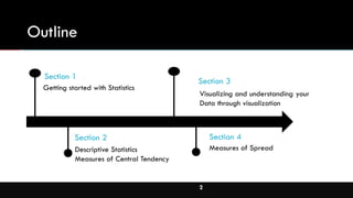
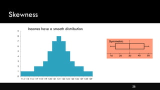
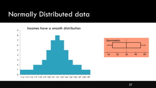
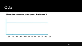
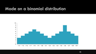
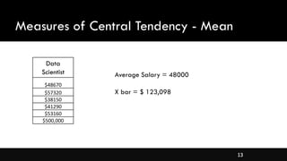
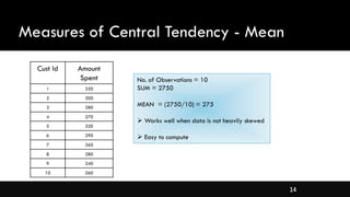
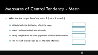
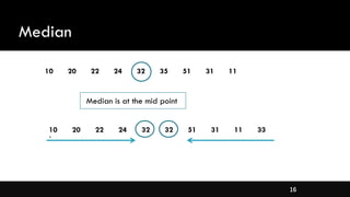
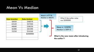
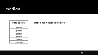
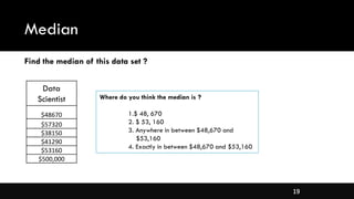
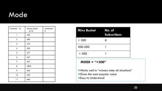
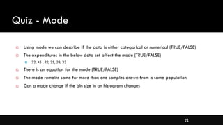
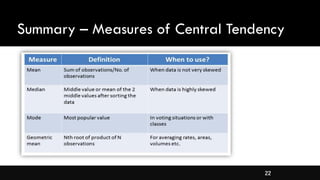
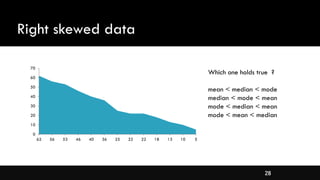
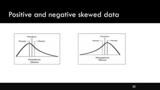
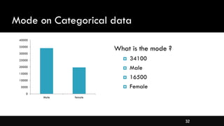
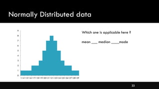
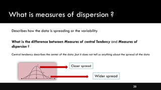
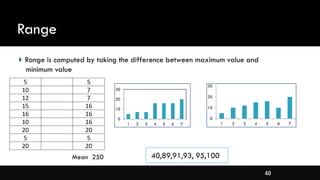
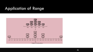
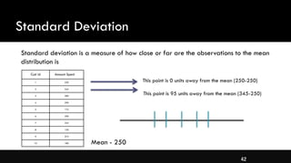
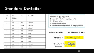
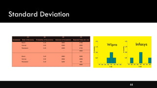
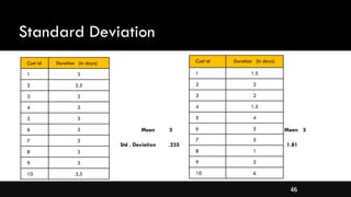
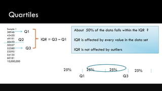
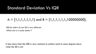
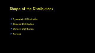
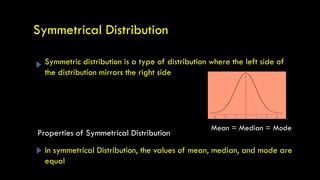
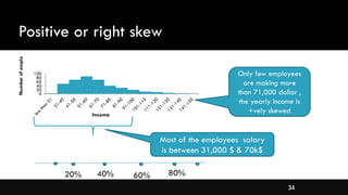
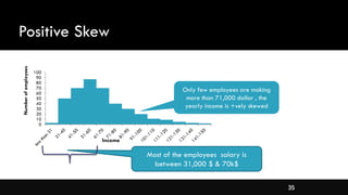
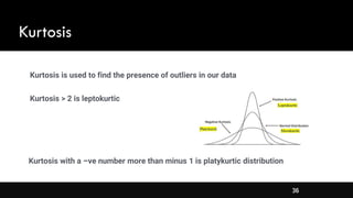
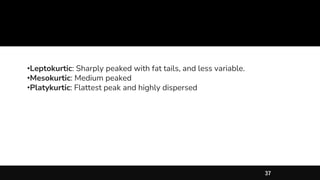
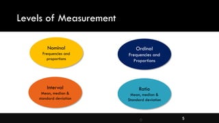
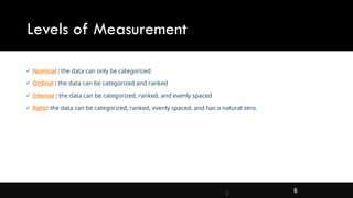
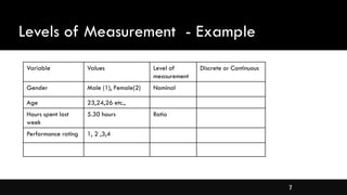
This document provides an outline and overview of descriptive statistics. It discusses the key concepts including: - Visualizing and understanding data through graphs and charts - Measures of central tendency like mean, median, and mode - Measures of spread like range, standard deviation, and interquartile range - Different types of distributions like symmetrical, skewed, and their properties - Levels of measurement for variables and appropriate statistics for each level The document serves as an introduction to descriptive statistics, the goals of which are to summarize key characteristics of data through numerical and visual methods.

1. Descriptive
Statistics

2. Outline
2
Section 1
Section 2 Section 4
Visualizing and understanding your
Data through visualization
Getting started with Statistics
Section 3
Descriptive Statistics
Measures of Central Tendency
Measures of Spread

3. 3
What is Statistics ?
It’s a science deals with Collection, Classification, Analysis , and Interpretation of
numerical facts or data AND the use of probability theory to impose order on aggregates
of data

4. 4
Branches of Statistics
Descriptive Statistics
Inferential Statistics

5. 0 5
Levels of Measurement
Nominal
Frequencies and
proportions
Ordinal
Frequencies and
Proportions
Interval
Mean, median &
standard deviation
Ratio
Mean, median &
Standard deviation

6. 0 6
Levels of Measurement
✓ Nominal : the data can only be categorized
✓ Ordinal : the data can be categorized and ranked
✓ Interval : the data can be categorized, ranked, and evenly spaced
✓ Ratio: the data can be categorized, ranked, evenly spaced, and has a natural zero.

7. 7
Levels of Measurement - Example
Variable Values Level of
measurement
Discrete or Continuous
Gender Male (1), Female(2) Nominal
Age 23,24,26 etc.,
Hours spent last
week
5.30 hours Ratio
Performance rating 1, 2 ,3,4

8. Descriptive Statistics

9. 9
Descriptive Statistics
Summarizing or describing the fact known to you Organizes and make sense
of Data uses Numerical and Graphical Methods Identifies Patterns in Data
Simplifies the information focusing on the items/areas of interest Eliminates
undesired information to avoid information overload

10. 10
Descriptive Statistics
Types of questions that can be answered using simple descriptive statistics:
1.What proportion of customers have responded to the offer in the dataset?
2.What is the average duration of calls? What is the median?
3.What is the frequency distribution of job types?

11. 11

12. 12
Measures of Central Tendency
Central tendency indicates where the centre of the distribution tends to be

13. 13
Measures of Central Tendency - Mean
Data
Scientist
$48670
$57320
$38150
$41290
$53160
$500,000
Average Salary = 48000
X bar = $ 123,098

14. 14
Measures of Central Tendency - Mean
Cust Id Amount
Spent
1 250
2 300
3 280
4 270
5 320
6 290
7 260
8 280
9 240
10 260
No. of Observations = 10
SUM = 2750
MEAN = (2750/10) = 275
➢ Works well when data is not heavily skewed
➢ Easy to compute

15. 15
Measures of Central Tendency - Mean
 What are the properties of the mean ? (put a tick mark )
 All salaries in the distribution affect the mean
 Mean can be described with a formula
 Many samples from the same population will have similar means
 The mean of a sample can be used to make inferences

16. 16
Median
10 20 22 24 32 35 51 31 11
Median is at the mid point
10
`
20 22 24 32 32 51 31 11 33

17. 17
Mean Vs Median
Data Scientist Data Analyst
58350 $48670
63120 $57320
44640 $38150
56380 $41290
72250 $53160
$500000
Mean is 47718
Median is 48670 What if the outlier value
was $500000
Mean is 123098
Median is 50915
What is the new mean after introducing
the outlier ?

18. 18
Median
What is the median value here ?
Data Scientist
$48670
$57320
$38150
$41290
$53160
$500,000

19. 19
Median
Data
Scientist
$48670
$57320
$38150
$41290
$53160
$500,000
Where do you think the median is ?
1.$ 48, 670
2. $ 53, 160
3. Anywhere in between $48,670 and
$53,160
4. Exactly in between $48,670 and $53,160
Find the median of this data set ?

20. 20
Mode
Customer id Amount Spent
(in $)
mins(bucke
t)
1 240
2 280
3 270
4 300
5 277
6 267
7 292
8 2800
9 260
10 250
11 480
Mins Bucket No. of
Subscribers
< 300 8
300-500 1
> 500 1
MODE = “<300”
Works well in “winners take all situations”
Gives the most popular value
Easy to Understand

21. 21
Quiz - Mode
 Using mode we can describe if the data is either categorical or numerical (TRUE/FALSE)
 The expenditures in the below data set affect the mode (TRUE/FALSE)
 32, 45 , 32, 25, 28, 32
 There is an equation for the mode (TRUE/FALSE)
 The mode remains same for more than one samples drawn from a same population
 Can a mode change if the bin size in an histogram changes

22. 22
Summary – Measures of Central Tendency

24. Symmetrical Distribution
Skewed Distribution
Uniform Distribution
Kurtosis
Shape of the Distributions

25. Symmetric distribution is a type of distribution where the left side of
the distribution mirrors the right side
Symmetrical Distribution
In symmetrical Distribution, the values of mean, median, and mode are
equal
Mean = Median = Mode
Properties of Symmetrical Distribution

26. 26
Skewness
0
1
2
3
4
5
6
7
8
9
114 115 116 117 118 119 120 121 121 123 124 125 126 127 128 129
Incomes have a smooth distribution

27. 27
Normally Distributed data
0
1
2
3
4
5
6
7
8
9
114 115 116 117 118 119 120 121 121 123 124 125 126 127 128 129
Incomes have a smooth distribution

28. 28
Right skewed data
0
10
20
30
40
50
60
70
62 56 53 46 40 36 25 22 22 18 13 10 5
Which one holds true ?
mean < median < mode
median < mode < mean
mode < median < mean
mode < mean < median

29. 29
Positive and negative skewed data

30. 30
Quiz
Where does the mode occur on this distribution ?
Jan Feb Mar Apr May Jun Jul Aug Sep Oct Nov Dec

31. 31
Mode on a binomial distribution
0
1
2
3
4
5
6
7
8
9
10
114 115 116 117 118 119 120 121 122 123 124 125 126 127 128 129

32. 32
Mode on Categorical data
0
5000
10000
15000
20000
25000
30000
35000
40000
Male female
What is the mode ?
 34100
 Male
 16500
 Female

33. 33
Normally Distributed data
0
1
2
3
4
5
6
7
8
9
114115116117118119120121121123124125126127128129
Which one is applicable here ?
mean ___ median ____mode

34. 34
Positive or right skew
0
20
40
60
80
100
Income
Number
of
employees
Only few employees
are making more
than 71,000 dollar ,
the yearly income is
+vely skewed
Most of the employees salary
is between 31,000 $ & 70k$
When the skewness statistic is +ve, the data is
right-skewed.
20% 40% 60% 80%

35. 35
Positive Skew
0
10
20
30
40
50
60
70
80
90
100
Income
Number
of
employees
Only few employees are making
more than 71,000 dollar , the
yearly income is +vely skewed
Most of the employees salary is
between 31,000 $ & 70k$

36. 36
Kurtosis
Kurtosis > 2 is leptokurtic
Kurtosis with a –ve number more than minus 1 is platykurtic distribution
Kurtosis is used to find the presence of outliers in our data

37. 37
•Leptokurtic: Sharply peaked with fat tails, and less variable.
•Mesokurtic: Medium peaked
•Platykurtic: Flattest peak and highly dispersed

38. Measures of
Dispersion

39. 39
What is measures of dispersion ?
Describes how the data is spreading or the variability
What is the difference between Measures of central Tendency and Measures of
dispersion ?
Central tendency describes the center of the data ,but it does not tell us anything about the spread of the data
Wider spread
Closer spread

40. 40
Range
Mean 250
5 5
10 7
12 7
15 16
16 16
10 16
20 20
5 5
20 20
0
10
20
30
1 2 3 4 5 6 7
0
10
20
30
1 2 3 4 5 6 7
40,89,91,93, 95,100
Range is computed by taking the difference between maximum value and
minimum value

41. 41
Application of Range

42. 42
Standard Deviation
Standard deviation is a measure of how close or far are the observations to the mean
distribution is
Cust id Amount Spent
1 250
2 345
3 280
4 290
5 175
6 200
7 255
8 150
9 375
10 180
This point is 0 units away from the mean (250-250)
This point is 95 units away from the mean (345-250)
Mean - 250

43. 43
Standard Deviation
Custo
mer
Id
Avg.
spend
(monthly)
x
x -µ (x -µ) ^2
1 304 69.2 4788.64
2 50 -184.8 34151.04
3 252 17.2 295.84
4 298 63.2 3994.24
5 234 -0.8 0.64
6 228 -6.8 46.24
7 264 29.2 852.64
8 230 -4.8 23.04
9 228 69.2 4788.64
10 260 -6.8 46.24
Mean = μ = 234.8
Variance = ∑(x – μ)^2/ N
Standard Deviation – sqrt(sigma^2)
X = Observation
μ = population mean
N = number of observations in the population
Variance =
Standard =
Deviation
Std Deviation = 22.13

44. 44
Standard Deviation
Wipro Infosys

45. 45
Standard Deviation
A startup ecommerce company has partnered with two different logistic company.
Not only the metropolitans even customers who lives in the remotest locations are demanding the same quality
and timeliness of the service. The constant challenge posed was in meeting pick up and delivery timelines
Of late, the ecommerce call center started receiving more complaints than in the past regarding delayed shipments
Logistic Company A Logistic Company B

46. 46
Standard Deviation
Cust id Duration (in days)
1 3
2 2.5
3 3
4 3
5 3
6 3
7 3
8 3
9 3
10 3.5
Cust id Duration (in days)
1 1.5
2 2
3 2
4 1.5
5 4
6 5
7 5
8 1
9 2
10 6
Mean 3 Mean 3
Std . Deviation .235 1.81

47. 47
Coefficient of Variation
Coefficient of variation is a measure of “the ratio of the standard deviation to
the arithmetic mean”
Coefficient of Variation = ((Standard deviation / Mean ) X 100) %
Purpose : This measure is used to compare the consistency of two or more groups in
the groups differ in their mean

48. 48
Chebyshev’s Theorem
Empirical(Normal) Rule: For a symmetrical, bell-shaped frequency distribution,
approximately 68 percent of the observations will lie within plus and minus one
standard deviation of the mean; about 95 percent of the observations will lie
within plus and minus two standard deviations of the mean; and practically all (99.7
percent) will lie within plus and minus three standard deviations of the mean.

49. 49
Chebyshev’s Theorem
68.5%
95.4%
99.8%

50. 50
Percentiles
Most commonly reported percentiles are quartiles, which break the data up into quarters
Sort the data
25th Percentile = 72.5
25th percentile can also be referred to as 1st quartile, Q1 , or the lower quartile
We have an even number of data , this means that when we calculate the
quartiles , we take the sum of the two values around each quartile and average
them

51. 51
Percentiles
50th Percentile = ?
50th percentile can also be referred as Median
83.5, it means that 50% of the data values fall at or below 83.5

52. 52
What is boxplot ?
It’s a visual representation which helps us to understand how spread the data and to
detect the outliers. In order to construct the same, we need min, Q1, median, Q3 and
the max value. To determine central tendency, spread, skewness, and the existence
of outliers.
Median
Upper Quartile
or
75th percentile
Lower Quartile
(or)
25th percentile
Min Max

53. 53
Percentiles
19 19 20 21 22 22 22 23 23 24 25
Q1
¼ or 25% of the data has a value that is less than or equal to 20
½ or 50% of the data has a value that is less than or equal to 22
¾ or 75% of data that has a value that is less than or equal to 23
½ or 50% of the data lies between 20 and 23
Q3
Depends on the context,
sometimes
Low percentile = good
High percentile = good

54. Boxplot Assignment
What is the 1st Quartile ?
What was the lowest sales achieved ?
What was the highest sales achieved ?
What was the median Sales achieved ?
The middle 50% of the sales achieved were between which scores ?
The majority of the sales were above 85 , true or false ?
Top 25% of the sales were between which two ranges ? :
70 75 77.5 80 85 87.5 90 95 100 105

55. Quartiles
Sample 1
38946
43420
49191
50430
50557
52580
53595
54135
60181
10,000,000
Q1
Q3
Q2 IQR = Q3 – Q1
About 50% of the data falls within the IQR ?
IQR is affected by every value in the data set
IQR is not affected by outliers
25% 25% 25% 25%
Q1 Q3

56. Standard Deviation Vs IQR
A = {1,1,1,1,1,1,1} and B = {1,1,1,1,1,1,100000000}.
IRQ for both is 0, but SD is very different.
Which one is is really better ?
It also shows that the IQR is very resistant to outliers (and to some degree skew)
while the SD is not

57. Good Luck