Downloaded 10 times

![Filter Design and Gibb’s Phenomenon
Objective:
In today’s Lab we will use different versions of
sinc function to design Low-pass, High-pass,
Band-pass, and band-stop filters. We will also
analyze the effect of length of h[n] on frequency
response and understand Gibb’s phenomenon.
Procedure:
1. Open M-file or M-Book
2. Save it by any useful name but remember not to
start the name by any numeric digit, do not use
any special character other than under-the-score
( _ ) and also remember not to give any space in
the name.
Gibb’s phenomenon occurs near a jump
discontinuity in the signal. It says that no
matter how many terms you include in your Fourier
series there will always be an error in the form
of an overshoot near the discontinuity. The
overshoot always be about 9% of the size of the
jump.
Task I:
3. Generate a sinc function with a zero crossing
frequency of 100 Hz and simulated sampling
frequency of 2500 Hz keeping index n=-100:100.
4. Analyze the Fourier transform of the signal
from step one using code from Lab2.
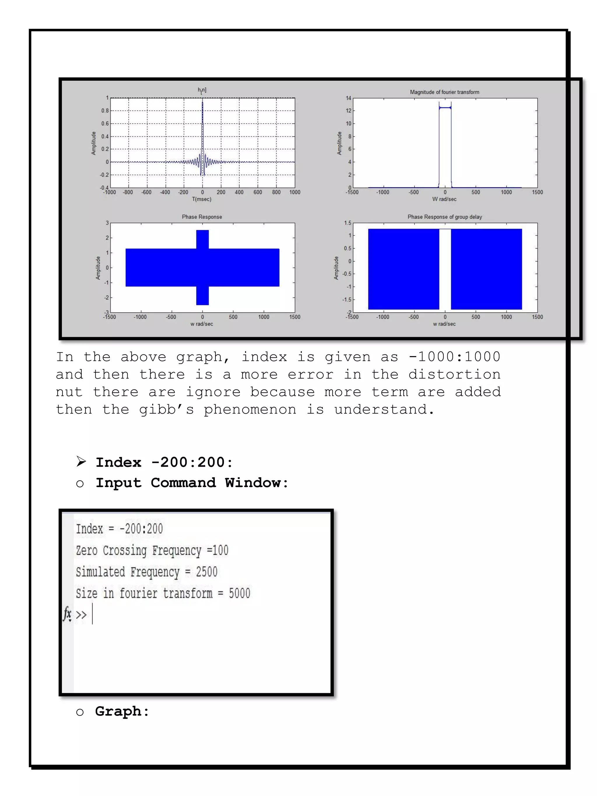
5. Now change the length of index to n=-200:200
and later to n=-1000:1000. While changing the
length continuously observe the effect on
magnitude of fft.](https://image.slidesharecdn.com/labreport9-170611122208/75/Filter-Designing-2-2048.jpg)
![6. You can also observe the wrapped and unwrapped
phase of the sinc function using angle and phase
command, respectively.
7. For calculating group delay take negative
derivative of the unwrapped phase, which shall be
approximate to 0.
Matlab Code:
Index =-100:100:
clc
close all
clear all
%Index
n=input('Index = ');
%Zero Crossing frequency
fc=input('Zero Crossing Frequency =');
%simulated frequency
fs=input('Simulated Frequency = ');
%size
N=input('Size in fourier transform = ');
%sinc function
h=sinc(2*fc/fs*n);
%plot the sinc function
subplot(221);
plot(n,h);
title('h_[n]');
grid on
ylabel 'Amplitude'
xlabel 'T(msec)'
%Omega Axis
w=linspace(-fs/2,fs/2,N);
%fourier transform
H=fftshift(fft(h,N));
%plot of Magnitude
subplot(222);
plot(w,abs(H));
title 'Magnitude of fourier transform'
ylabel 'Amplitude'
xlabel 'W rad/sec'
%plot Phase response
subplot(223);
plot(w,angle(H));](https://image.slidesharecdn.com/labreport9-170611122208/75/Filter-Designing-3-2048.jpg)


![%simulated frequency
fs=input('Simulated Frequency = ');
%size
N=input('Size in fourier transform = ');
%sinc function
h=sinc(2*fc/fs*n).*exp(-1i*pi*n);
%plot the sinc function
subplot(221);
plot(n,h);
title('h[n]');
grid on
ylabel 'Amplitude'
xlabel 'T(msec)'
%Omega Axis
w=linspace(-fs/2,fs/2,N);
%fourier transform
H=fftshift(fft(h,N));
%plot of Magnitude
subplot(222);
plot(w,abs(H));
title 'Magnitude of fourier transform'
ylabel 'Amplitude'
xlabel 'W rad/sec'
%plot Phase response
subplot(223);
plot(w,angle(H));
title 'Phase Response'
ylabel 'Amplitude'
xlabel 'w rad/sec'
%plot group delay
subplot(224);
plot(w(1:4999),-diff(phase(H)));
title 'Phase Response of group delay'
ylabel 'Amplitude'
xlabel 'w rad/sec'
Output:
Index =-100:100:
o Input Comand Window:](https://image.slidesharecdn.com/labreport9-170611122208/75/Filter-Designing-8-2048.jpg)


![exponential is shifting in the fourier transform
and more jums are occur and error are increasing.
Multiply Cos(2*pi/2*n):
Matlab Code:
clc
close all
clear all
%Index
n=input('Index = ');
%Zero Crossing frequency
fc=input('Zero Crossing Frequency =');
%simulated frequency
fs=input('Simulated Frequency = ');
%size
N=input('Size in fourier transform = ');
%sinc function
h=sinc(2*fc/fs*n).*cos(2*(pi/2)*n);
%plot the sinc function
subplot(221);
plot(n,h);
title('h[n]');
grid on
ylabel 'Amplitude'
xlabel 'T(msec)'
%Omega Axis
w=linspace(-fs/2,fs/2,N);
%fourier transform
H=fftshift(fft(h,N));
%plot of Magnitude
subplot(222);
plot(w,abs(H));
title 'Magnitude of fourier transform'
ylabel 'Amplitude'
xlabel 'W rad/sec'
%plot Phase response
subplot(223);
plot(w,angle(H));
title 'Phase Response'
ylabel 'Amplitude'
xlabel 'w rad/sec'
%plot group delay
subplot(224);
plot(w(1:4999),-diff(phase(H)));
title 'Phase Response of group delay'
ylabel 'Amplitude'
xlabel 'w rad/sec'](https://image.slidesharecdn.com/labreport9-170611122208/75/Filter-Designing-11-2048.jpg)


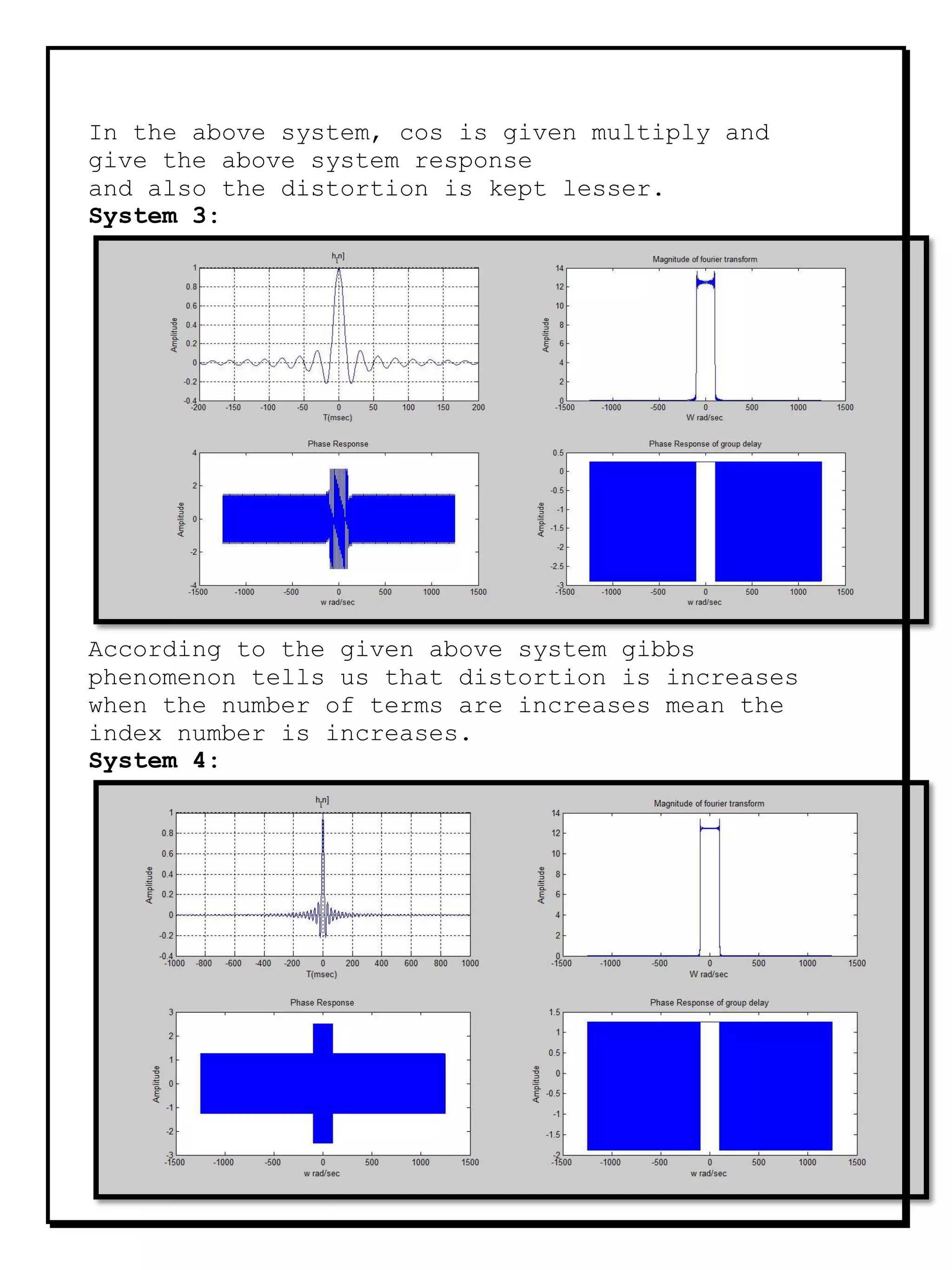


1) The document describes a digital signal processing lab report that analyzes Gibbs phenomenon using different sinc functions to design filters. 2) The lab uses sinc functions with varying indices to design low-pass, high-pass, band-pass and band-stop filters. The effect of the sinc function length on frequency response and Gibbs phenomenon is observed. 3) Gibbs phenomenon occurs near discontinuities, where the Fourier series approximation will always have an error in the form of an overshoot near the discontinuity, about 9% of the size of the jump, no matter how many terms are used.