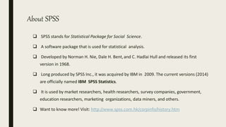
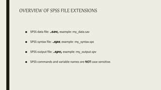
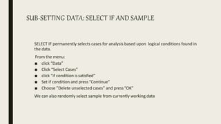
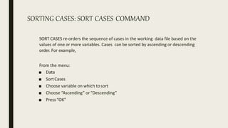
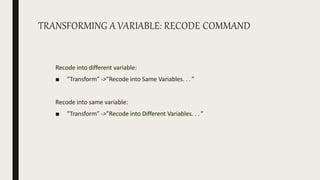
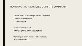
An Introduction to SPSS
Md. Shahbaz Alam
Email: salam6@isrt.ac.bd
Session Outline
 Introduction
 Getting Started with SPSS
 Data Management
 Basic Analysis
 Hypothesis Testing
Introduction
About SPSS
 SPSS stands for Statistical Package for Social Science.
 A software package that is used for statistical analysis.
 Developed by Norman H. Nie, Dale H. Bent,and C. Hadlai Hull and released its first
version in 1968.
 Long produced by SPSS Inc., it was acquired by IBM in 2009. The current versions (2014)
are officially named IBM SPSS Statistics.
 It is used by market researchers, health researchers, survey companies, government,
education researchers, marketing organizations, data miners, and others.
 Want to know more! Visit: http://www.spss.com.hk/corpinfo/history.htm
OVERVIEW OF SPSS FILE EXTENSIONS
■ SPSS data file: .sav, example: my_data.sav
■ SPSS syntax file: .sps, example: my_syntax.sps
■ SPSS output file: .spv, example: my_output.spv
■ SPSS commands and variable names are NOTcase sensitive.
RULES FOR VARIABLE NAMING
 The name must begin with a letter. The remaining characters can be any
letter, any digit, a period, or the symbols @, #, _, or $.
 Blanks and special characters (for example, !, ?, ‘, and *) cannot be used.
 Reserved keywords cannot be used as variable names.
 Reserved keywords are: ALL, AND, BY, EQ, GE, GT, LE, LT, NE, NOT, OR, TO,
WITH.
 Variable names cannot end with a period (.) since the period may be
interpreted as a command terminator.
 Variable names should not contain more than 64 characters.
SPSS Windows
Getting Started with
SPSS
Opening SPSS
■ The default window will have the data editor
■ There are two sheets in the window:
1. Data view 2. Variable view
Data View window
■ The Data View window
This sheet is visible when you first open the Data Editor and this sheet contains the data
■ Click on the tab labeled Variable View
Variable View window
■ This sheet contains information about the data set that is stored with the dataset
■ Name
– The first character of the variable name must be alphabetic
– Variable names must be unique, and have to be less than 64 characters.
– Spaces are NOT allowed.
Variable View window
■ Type
– Click on the ‘type’ box. The two basic types of variables that we will use are
numeric and string. This column enables us to specify the type of variable.
Variable View window
■ Width
– Width allows us to determine the number of characters SPSS
will allow to be entered for the variable
Variable View window
■ Decimals
– Number of decimals
– It has to be less than or equal to 16
Variable View window
■ Label
– You can specify the details of the variable
– You can write characters with spaces up to 256 characters
Variable View window
■ Values
– This is used and to suggest which numbers represent which categories when
the variable represents a category
Defining the value labels
■ Click the cell in the values column as shown below
■ For the value, and the label, you can put up to 60 characters.
■ After defining the values click add and then click OK.
Output Viewer
Displays output and errors. Extension of the saved file will be “.spv”
Practice 1
■ How would you put the following information into SPSS?
Name Gender Height
A male 5.7
B female 5.4
C female 5.3
D male 5.6
E male 5.8
F male 5.7
G female 5.5
H female 5.5
I female 5.6
J male 6
Practice 1 (Solution Sample)
Click
Saving the data
■ To save the data file you created simply click ‘file’ and click ‘save as.’ You can save
the file in different forms by clicking “Save as type.”
OPENING DATA, SYNTAXES AND OUTPUTS IN SPSS
IMPORTING EXCEL DATA FILES INTO SPSS
ARITHMETIC, RELATIONAL AND LOGICAL OPERATORS
Arithmetic operator
Addition (+), Subtraction (-),
Multiplication (*), Division (/), Exponentiation
(**).
Relational operator
Equal to (EQ or =),
Not equal to (NE or ∟=),
Less than (LT or <),
Less than or equal to (LE or <=),
Greater than (GT or >),
Greater than or equal to (GE or >=).
Logical operator AND and OR.
Missing value function MISSING(arg), SYSMIS(arg)
Data Management
SUB-SETTING DATA: SELECT IF AND SAMPLE
SELECT IF permanently selects cases for analysis based upon logical conditions found in
the data.
From the menu:
■ click “Data”
■ Click “Select Cases”
■ click “if condition issatisfied”
■ Set if condition and press“Continue”
■ Choose ”Delete unselected cases” and press“OK”
We can also randomly select sample from currently working data
SORTING CASES: SORT CASES COMMAND
SORT CASES re-orders the sequence of cases in the working data file based on the
values of one or more variables. Cases can be sorted by ascending or descending
order. For example,
From the menu:
■ Data
■ SortCases
■ Choose variable on which tosort
■ Choose “Ascending” or“Descending”
■ Press“OK”
TRANSFORMING A VARIABLE: RECODE COMMAND
Recode into different variable:
■ ”Transform” ->”Recode into Same Variables. . . ”
Recode into same variable:
■ ”Transform” ->”Recode into Different Variables. . . ”
TRANSFORMING A VARIABLE: COMPUTE COMMAND
General form: COMPUTE target variable = expression
Compute salary increment:
SALARY-SALBEGIN
Compute % of increment:
PINCREM=(INCREMENT/SALBEGIN)* 100.
Then compute salary increase for the next year:
RAISE = SALARY * 0.12.
TRANSFORMING A VARIABLE: COMPUTE COMMAND
From the menu:
■ Go to “Compute Variable” from “Transform”menu
■ Name “TargetVariable”
■ Set “NumericExpression”
■ Follow steps and finally press“OK”
APPENDING AND MERGING SPSS DATA FILES
 Append: Adding additional observations to an existing data set.
 Merge: Adding additional variables to an existing data set. Need to sort the common
variable(in both dataset) first.
Basic Analysis
Some Basic Analysis in SPSS
■ Frequencies
– Produces frequency tables that shows frequency counts and percentages of
the values of individual variables.
■ Descriptives
– This analysis shows the summary statistics( maximum, minimum, mean,
standard deviation etc.) of the variables.
■ Linear regression analysis
– Linear Regression estimates the coefficients of the linear equation
Frequencies
We want to draw a frequency table as well as a bar chart for ‘Gender’ variable
From the menu:
 Click ‘Analyze’ , ‘Descriptive statistics,’ then click ‘Frequencies’
Frequencies
■ Click gender and put it into the variable box.
■ Click ‘Charts.’
■ Then click ‘Bar charts’ and click ‘Continue.’
Click
Frequencies
■ Finally Click OK in the Frequencies box.
Click
Output
Practice 2
■ Do a frequency analysis on the variable “minority”
■ Create a pie charts for it
Answer
Answer
Practice 3
■ Draw a histogram for the variable ‘salary’
■ Also show a table that contains summary statistics like
mean, median, minimum and maximum salary.
Answer
Descriptives
■ Click ‘Analyze,’ ‘Descriptive statistics,’ then click ‘Descriptives’
■ Click ‘Educational level’ and ‘Beginning Salary,’ and put it into the
variable box.
■ Click Options
Click
Descriptives
■ The options allows you to analyze other descriptive statistics besides the mean
and Std.
■ Click ‘variance’ and ‘kurtosis’
■ Finally click ‘Continue’
Click
Click
Descriptives
■ Finally Click OK in the Descriptives box. You will be able to see the result of the
analysis.
Regression Analysis
■ Click ‘Analyze,’ ‘Regression,’ then click ‘Linear’ from the main menu.
Regression Analysis
■ For example let’s analyze the model
■ Put ‘Current Salary’ as Dependent and ‘Previous Salary’ as Independent
variable.
Click Click
Regression Analysis
■ Clicking OK gives the result.
Plotting the Regression Line
■ Click ‘Graphs,’ ‘Legacy Dialogs,’ ‘Interactive,’ and ‘Scatterplot’
from the main menu.
Plotting the Regression Line
■ Drag ‘Current Salary’ into the vertical axis box and ‘Beginning Salary’ in the
horizontal axis box.
■ Click ‘Fit’ bar. Make sure the Method is regression in the Fit box. Then click ‘OK’.
Click
Set this to
Regression!
Output
Practice 4
■ Find out whether or not the previous experience of workers has any affect on their
beginning salary?
– Take the variable “salbegin,” and “prevexp” as dependent and independent
variables respectively.
■ Plot the regression line for the above analysis using the “scatter plot” menu.
Output
Output
Test of Hypothesis
Basics of Hypothesis Testing
Hypothesis Testing is a decision making process
for evaluating claims about a population.
Basics of Hypothesis Testing
The researcher must
1) Define the population under study
2) State the hypothesis that is under investigation
3) Give the significance level
4) Select a sample from the population
5) Collect the data
6) Perform the statistical test
7) Reach a conclusion
Basics of Hypothesis Testing
How to set your hypotheses
1) Set the researcher’s hypothesis as alternative
hypothesis.
2) When you are testing if a parameter differs from a certain value, set
that particular value as the null value.
3) If you are testing a difference between two samples, set
0 as the null value.
Basics of Hypothesis Testing
• Decisions are taken based on P-values.
• P-value stands for probability value.
Definition of P-value
The probability of observing more extreme observations (or observing more extreme
test statistics).
Basics of Hypothesis Testing
One-tailed test
e.g.
H0: Âľ1 = Âľ2
H1: Âľ1 > Âľ2
If the sample
statistic falls
in this region,
we would
not reject H0.
We would reject
H0 if the sample
statistic falls in
these regions.
Basics of Hypothesis Testing
• The area of the rejection region is α.
• α is called the level of significance.
Youreject your null hypothesis when the p-value is lower than Îą i.e. there is more
chance of observing more extreme observations than those obtained from the
sample.
One sample t-test (Test of Population Mean)
Suppose that we want to answer the question: Can you conclude that a certain
population mean is not 50? The null hypothesis is
H0: Âľ = 50
and the alternative hypothesis is
H1: µ ≠ 50.
One sample t-test (Test of Population Mean)
For example, using the hsb2.sav data file, say we wish to test whether the average
writing score (write) differs significantly from 50. Wecan do this as shown below.
• Click ‘Analyze’, ‘compare means’ then click ‘one sample t-test’
• Put the variable that we wish to test in the ‘Test Variable(s)’ box
• Set the test value. (say 50)
• Click ‘OK’
One sample t-test (Test of Population Mean)
Output:
In a similar way we can perform two sample t-test
Test of Association
Suppose we want to test if a categorical variable is associated with another categorical
variable. We first make a contingency table and perform Chi- square test of
association. Wemay state the hypothesis formally as follows:
H0: No association
H1: There is association
Test of Association
Test of Association
Using the hsb2.sav data file, let's see if there is a relationship between the type
of school attended (schtyp) and students' gender (female). Remember that the
chi-square test assumes that the expected value for each cell is five or higher.We
can dothis as follows:
• Click‘Analyze’,go to ‘Descriptive statistics’and then click
‘crosstabs.’
• Put Rowand Columnvariablein the boxthen click ‘Statistics’.Select Chi-
square,then click ‘continue’,then ‘ok’
Test of Association
Test of Association
Output:
Decision: These results indicate that there is no statistically significant relationship between
the type of school attended and gender.
Thank you for your
patience!

An introduction to spss

  • 1.
    An Introduction toSPSS Md. Shahbaz Alam Email: salam6@isrt.ac.bd
  • 2.
    Session Outline  Introduction Getting Started with SPSS  Data Management  Basic Analysis  Hypothesis Testing
  • 3.
  • 4.
    About SPSS  SPSSstands for Statistical Package for Social Science.  A software package that is used for statistical analysis.  Developed by Norman H. Nie, Dale H. Bent,and C. Hadlai Hull and released its first version in 1968.  Long produced by SPSS Inc., it was acquired by IBM in 2009. The current versions (2014) are officially named IBM SPSS Statistics.  It is used by market researchers, health researchers, survey companies, government, education researchers, marketing organizations, data miners, and others.  Want to know more! Visit: http://www.spss.com.hk/corpinfo/history.htm
  • 5.
    OVERVIEW OF SPSSFILE EXTENSIONS ■ SPSS data file: .sav, example: my_data.sav ■ SPSS syntax file: .sps, example: my_syntax.sps ■ SPSS output file: .spv, example: my_output.spv ■ SPSS commands and variable names are NOTcase sensitive.
  • 6.
    RULES FOR VARIABLENAMING  The name must begin with a letter. The remaining characters can be any letter, any digit, a period, or the symbols @, #, _, or $.  Blanks and special characters (for example, !, ?, ‘, and *) cannot be used.  Reserved keywords cannot be used as variable names.  Reserved keywords are: ALL, AND, BY, EQ, GE, GT, LE, LT, NE, NOT, OR, TO, WITH.  Variable names cannot end with a period (.) since the period may be interpreted as a command terminator.  Variable names should not contain more than 64 characters.
  • 7.
  • 8.
  • 9.
    Opening SPSS ■ Thedefault window will have the data editor ■ There are two sheets in the window: 1. Data view 2. Variable view
  • 10.
    Data View window ■The Data View window This sheet is visible when you first open the Data Editor and this sheet contains the data ■ Click on the tab labeled Variable View
  • 11.
    Variable View window ■This sheet contains information about the data set that is stored with the dataset ■ Name – The first character of the variable name must be alphabetic – Variable names must be unique, and have to be less than 64 characters. – Spaces are NOT allowed.
  • 12.
    Variable View window ■Type – Click on the ‘type’ box. The two basic types of variables that we will use are numeric and string. This column enables us to specify the type of variable.
  • 13.
    Variable View window ■Width – Width allows us to determine the number of characters SPSS will allow to be entered for the variable
  • 14.
    Variable View window ■Decimals – Number of decimals – It has to be less than or equal to 16
  • 15.
    Variable View window ■Label – You can specify the details of the variable – You can write characters with spaces up to 256 characters
  • 16.
    Variable View window ■Values – This is used and to suggest which numbers represent which categories when the variable represents a category
  • 17.
    Defining the valuelabels ■ Click the cell in the values column as shown below ■ For the value, and the label, you can put up to 60 characters. ■ After defining the values click add and then click OK.
  • 18.
    Output Viewer Displays outputand errors. Extension of the saved file will be “.spv”
  • 19.
    Practice 1 ■ Howwould you put the following information into SPSS? Name Gender Height A male 5.7 B female 5.4 C female 5.3 D male 5.6 E male 5.8 F male 5.7 G female 5.5 H female 5.5 I female 5.6 J male 6
  • 20.
    Practice 1 (SolutionSample) Click
  • 21.
    Saving the data ■To save the data file you created simply click ‘file’ and click ‘save as.’ You can save the file in different forms by clicking “Save as type.”
  • 22.
    OPENING DATA, SYNTAXESAND OUTPUTS IN SPSS
  • 23.
    IMPORTING EXCEL DATAFILES INTO SPSS
  • 24.
    IMPORTING EXCEL DATAFILES INTO SPSS
  • 25.
    ARITHMETIC, RELATIONAL ANDLOGICAL OPERATORS Arithmetic operator Addition (+), Subtraction (-), Multiplication (*), Division (/), Exponentiation (**). Relational operator Equal to (EQ or =), Not equal to (NE or ∟=), Less than (LT or <), Less than or equal to (LE or <=), Greater than (GT or >), Greater than or equal to (GE or >=). Logical operator AND and OR. Missing value function MISSING(arg), SYSMIS(arg)
  • 26.
  • 27.
    SUB-SETTING DATA: SELECTIF AND SAMPLE SELECT IF permanently selects cases for analysis based upon logical conditions found in the data. From the menu: ■ click “Data” ■ Click “Select Cases” ■ click “if condition issatisfied” ■ Set if condition and press“Continue” ■ Choose ”Delete unselected cases” and press“OK” We can also randomly select sample from currently working data
  • 28.
    SORTING CASES: SORTCASES COMMAND SORT CASES re-orders the sequence of cases in the working data file based on the values of one or more variables. Cases can be sorted by ascending or descending order. For example, From the menu: ■ Data ■ SortCases ■ Choose variable on which tosort ■ Choose “Ascending” or“Descending” ■ Press“OK”
  • 29.
    TRANSFORMING A VARIABLE:RECODE COMMAND Recode into different variable: ■ ”Transform” ->”Recode into Same Variables. . . ” Recode into same variable: ■ ”Transform” ->”Recode into Different Variables. . . ”
  • 30.
    TRANSFORMING A VARIABLE:COMPUTE COMMAND General form: COMPUTE target variable = expression Compute salary increment: SALARY-SALBEGIN Compute % of increment: PINCREM=(INCREMENT/SALBEGIN)* 100. Then compute salary increase for the next year: RAISE = SALARY * 0.12.
  • 31.
    TRANSFORMING A VARIABLE:COMPUTE COMMAND From the menu: ■ Go to “Compute Variable” from “Transform”menu ■ Name “TargetVariable” ■ Set “NumericExpression” ■ Follow steps and finally press“OK”
  • 32.
    APPENDING AND MERGINGSPSS DATA FILES  Append: Adding additional observations to an existing data set.  Merge: Adding additional variables to an existing data set. Need to sort the common variable(in both dataset) first.
  • 33.
  • 34.
    Some Basic Analysisin SPSS ■ Frequencies – Produces frequency tables that shows frequency counts and percentages of the values of individual variables. ■ Descriptives – This analysis shows the summary statistics( maximum, minimum, mean, standard deviation etc.) of the variables. ■ Linear regression analysis – Linear Regression estimates the coefficients of the linear equation
  • 35.
    Frequencies We want todraw a frequency table as well as a bar chart for ‘Gender’ variable From the menu:  Click ‘Analyze’ , ‘Descriptive statistics,’ then click ‘Frequencies’
  • 36.
    Frequencies ■ Click genderand put it into the variable box. ■ Click ‘Charts.’ ■ Then click ‘Bar charts’ and click ‘Continue.’ Click
  • 37.
    Frequencies ■ Finally ClickOK in the Frequencies box. Click
  • 38.
  • 39.
    Practice 2 ■ Doa frequency analysis on the variable “minority” ■ Create a pie charts for it
  • 40.
  • 41.
  • 42.
    Practice 3 ■ Drawa histogram for the variable ‘salary’ ■ Also show a table that contains summary statistics like mean, median, minimum and maximum salary.
  • 43.
  • 44.
    Descriptives ■ Click ‘Analyze,’‘Descriptive statistics,’ then click ‘Descriptives’ ■ Click ‘Educational level’ and ‘Beginning Salary,’ and put it into the variable box. ■ Click Options Click
  • 45.
    Descriptives ■ The optionsallows you to analyze other descriptive statistics besides the mean and Std. ■ Click ‘variance’ and ‘kurtosis’ ■ Finally click ‘Continue’ Click Click
  • 46.
    Descriptives ■ Finally ClickOK in the Descriptives box. You will be able to see the result of the analysis.
  • 47.
    Regression Analysis ■ Click‘Analyze,’ ‘Regression,’ then click ‘Linear’ from the main menu.
  • 48.
    Regression Analysis ■ Forexample let’s analyze the model ■ Put ‘Current Salary’ as Dependent and ‘Previous Salary’ as Independent variable. Click Click
  • 49.
  • 50.
    Plotting the RegressionLine ■ Click ‘Graphs,’ ‘Legacy Dialogs,’ ‘Interactive,’ and ‘Scatterplot’ from the main menu.
  • 51.
    Plotting the RegressionLine ■ Drag ‘Current Salary’ into the vertical axis box and ‘Beginning Salary’ in the horizontal axis box. ■ Click ‘Fit’ bar. Make sure the Method is regression in the Fit box. Then click ‘OK’. Click Set this to Regression!
  • 52.
  • 53.
    Practice 4 ■ Findout whether or not the previous experience of workers has any affect on their beginning salary? – Take the variable “salbegin,” and “prevexp” as dependent and independent variables respectively. ■ Plot the regression line for the above analysis using the “scatter plot” menu.
  • 54.
  • 55.
  • 56.
  • 57.
    Basics of HypothesisTesting Hypothesis Testing is a decision making process for evaluating claims about a population.
  • 58.
    Basics of HypothesisTesting The researcher must 1) Define the population under study 2) State the hypothesis that is under investigation 3) Give the significance level 4) Select a sample from the population 5) Collect the data 6) Perform the statistical test 7) Reach a conclusion
  • 59.
    Basics of HypothesisTesting How to set your hypotheses 1) Set the researcher’s hypothesis as alternative hypothesis. 2) When you are testing if a parameter differs from a certain value, set that particular value as the null value. 3) If you are testing a difference between two samples, set 0 as the null value.
  • 60.
    Basics of HypothesisTesting • Decisions are taken based on P-values. • P-value stands for probability value. Definition of P-value The probability of observing more extreme observations (or observing more extreme test statistics).
  • 61.
    Basics of HypothesisTesting One-tailed test e.g. H0: Âľ1 = Âľ2 H1: Âľ1 > Âľ2 If the sample statistic falls in this region, we would not reject H0. We would reject H0 if the sample statistic falls in these regions.
  • 62.
    Basics of HypothesisTesting • The area of the rejection region is α. • α is called the level of significance. Youreject your null hypothesis when the p-value is lower than α i.e. there is more chance of observing more extreme observations than those obtained from the sample.
  • 63.
    One sample t-test(Test of Population Mean) Suppose that we want to answer the question: Can you conclude that a certain population mean is not 50? The null hypothesis is H0: µ = 50 and the alternative hypothesis is H1: µ ≠ 50.
  • 64.
    One sample t-test(Test of Population Mean) For example, using the hsb2.sav data file, say we wish to test whether the average writing score (write) differs significantly from 50. Wecan do this as shown below. • Click ‘Analyze’, ‘compare means’ then click ‘one sample t-test’ • Put the variable that we wish to test in the ‘Test Variable(s)’ box • Set the test value. (say 50) • Click ‘OK’
  • 65.
    One sample t-test(Test of Population Mean) Output: In a similar way we can perform two sample t-test
  • 66.
    Test of Association Supposewe want to test if a categorical variable is associated with another categorical variable. We first make a contingency table and perform Chi- square test of association. Wemay state the hypothesis formally as follows: H0: No association H1: There is association
  • 67.
  • 68.
    Test of Association Usingthe hsb2.sav data file, let's see if there is a relationship between the type of school attended (schtyp) and students' gender (female). Remember that the chi-square test assumes that the expected value for each cell is five or higher.We can dothis as follows: • Click‘Analyze’,go to ‘Descriptive statistics’and then click ‘crosstabs.’ • Put Rowand Columnvariablein the boxthen click ‘Statistics’.Select Chi- square,then click ‘continue’,then ‘ok’
  • 69.
  • 70.
    Test of Association Output: Decision:These results indicate that there is no statistically significant relationship between the type of school attended and gender.
  • 71.
    Thank you foryour patience!