Downloaded 47 times
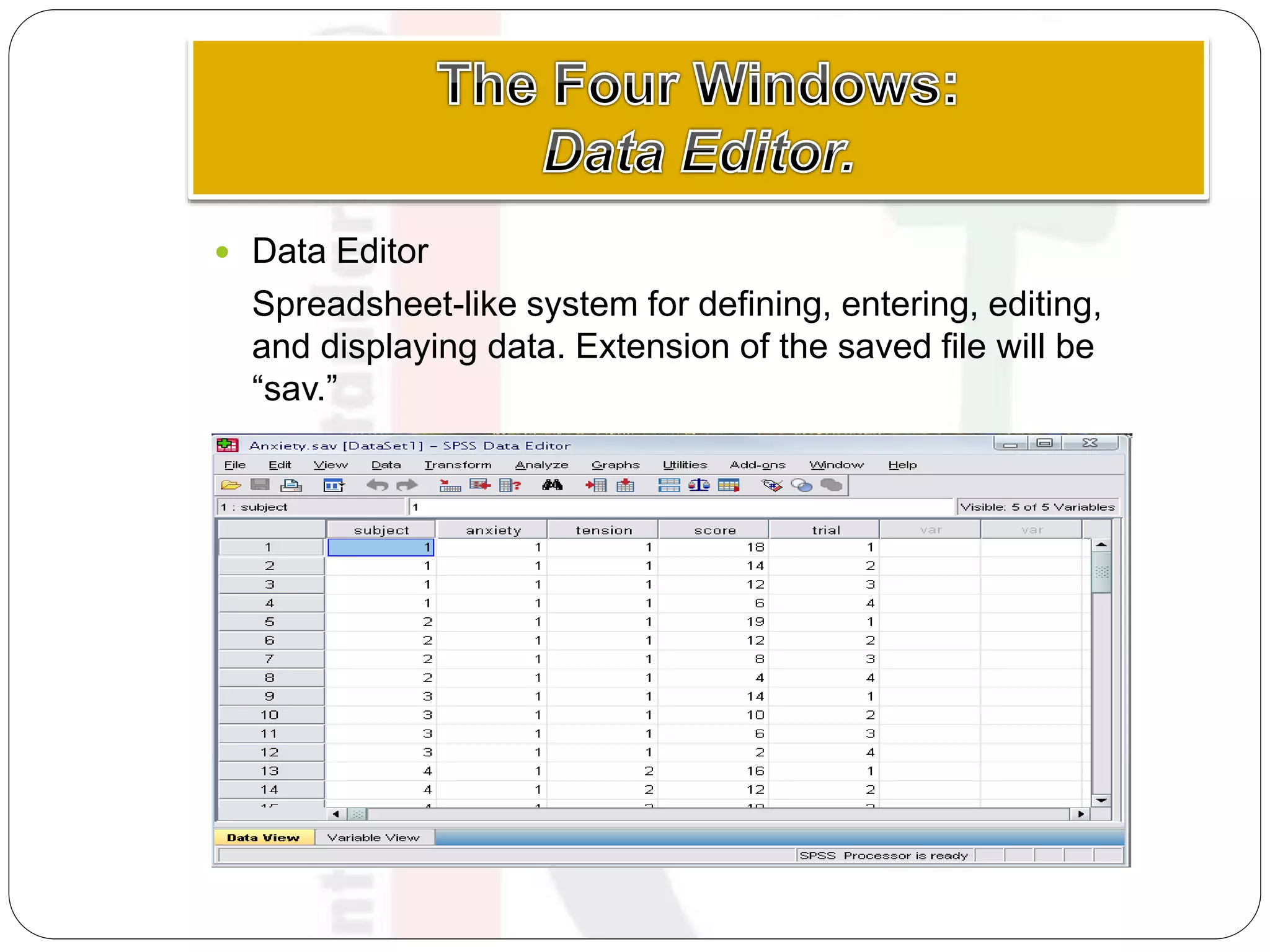
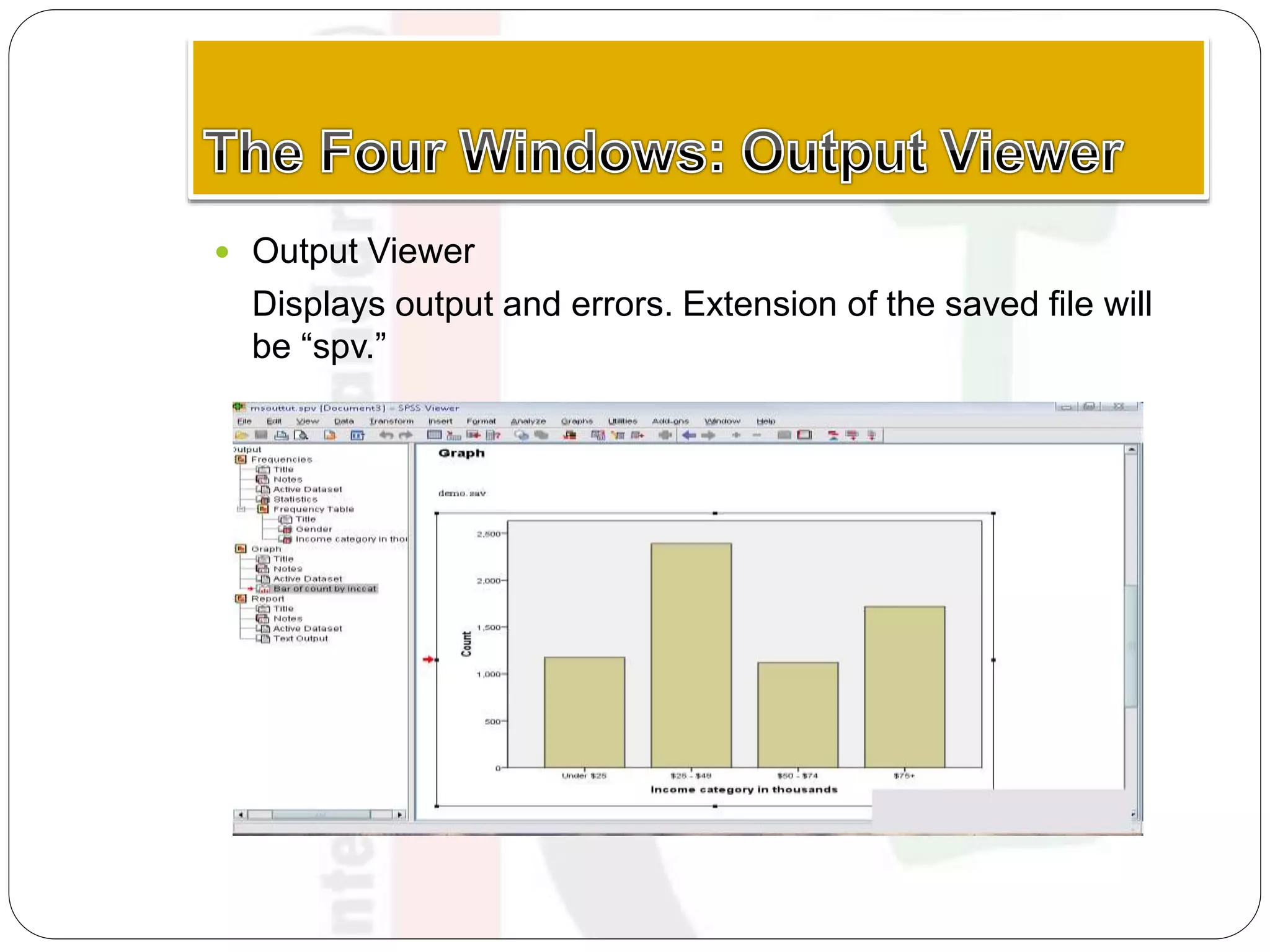
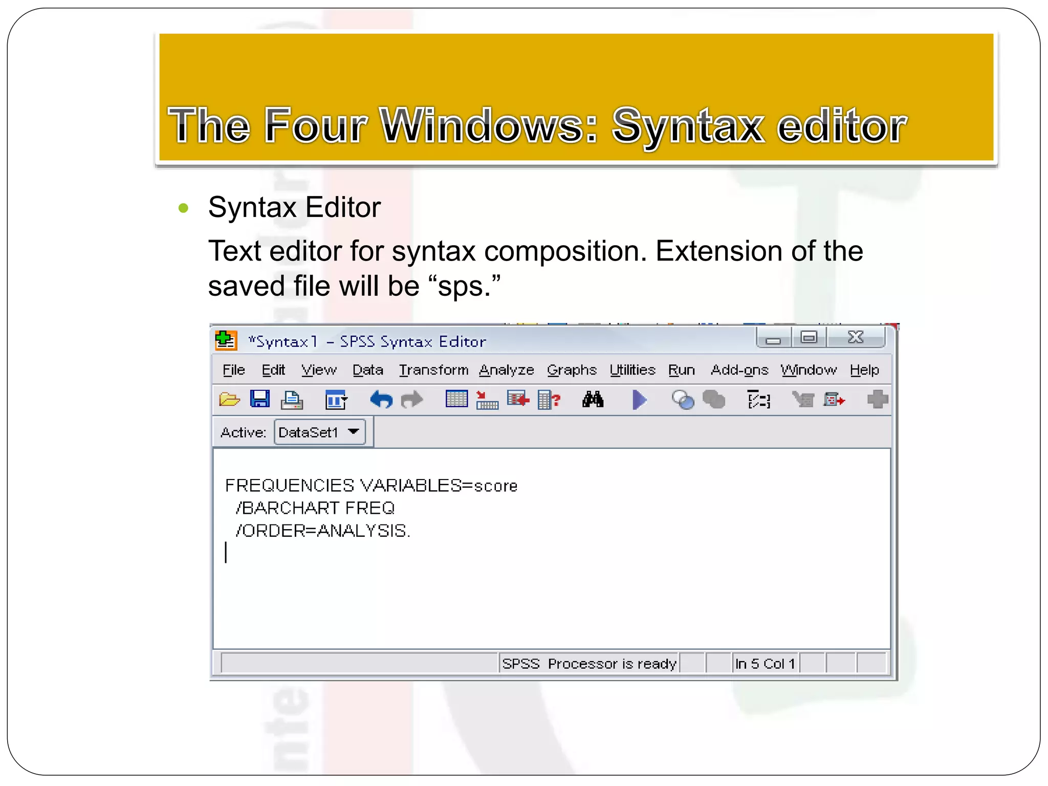
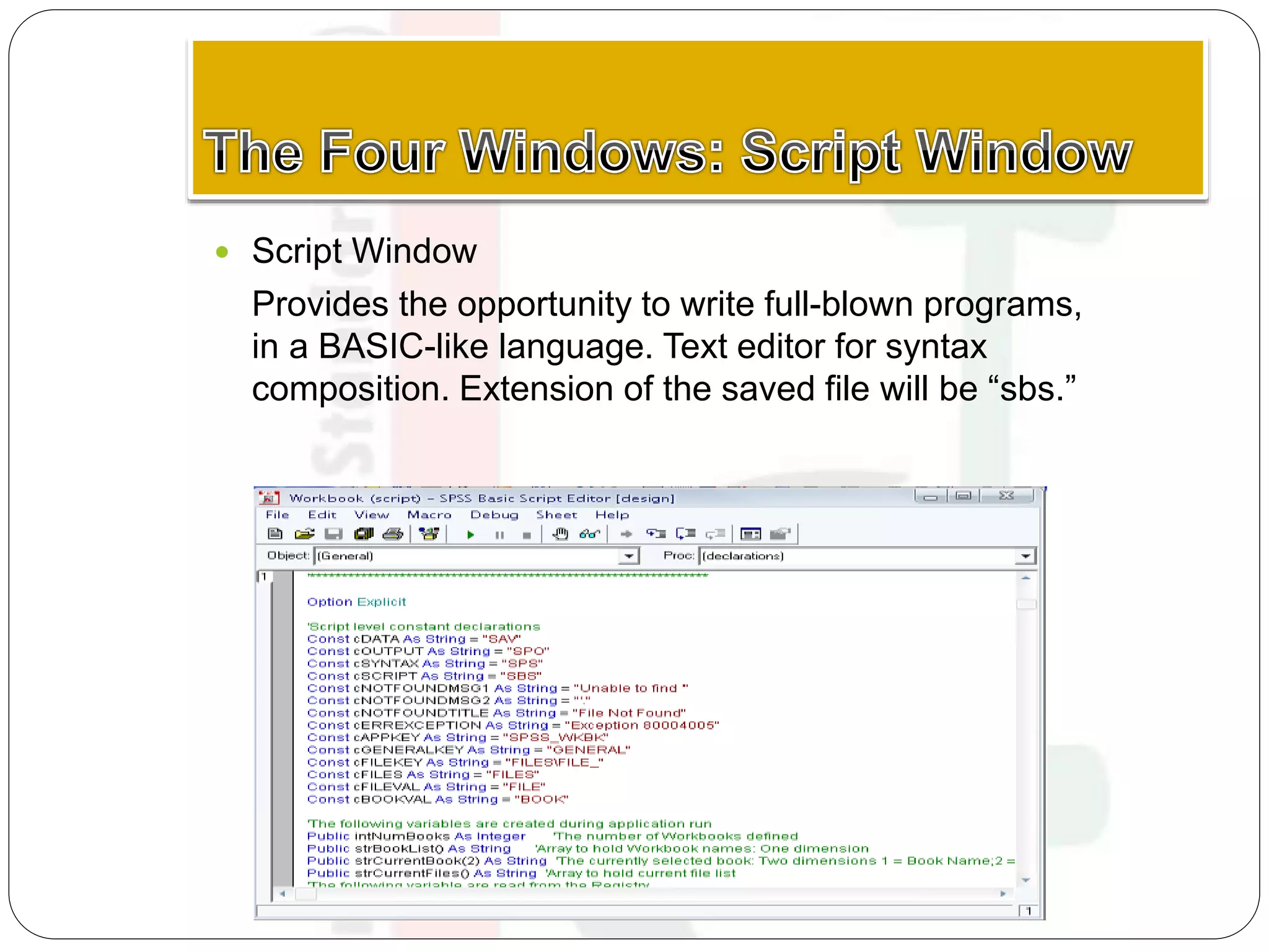
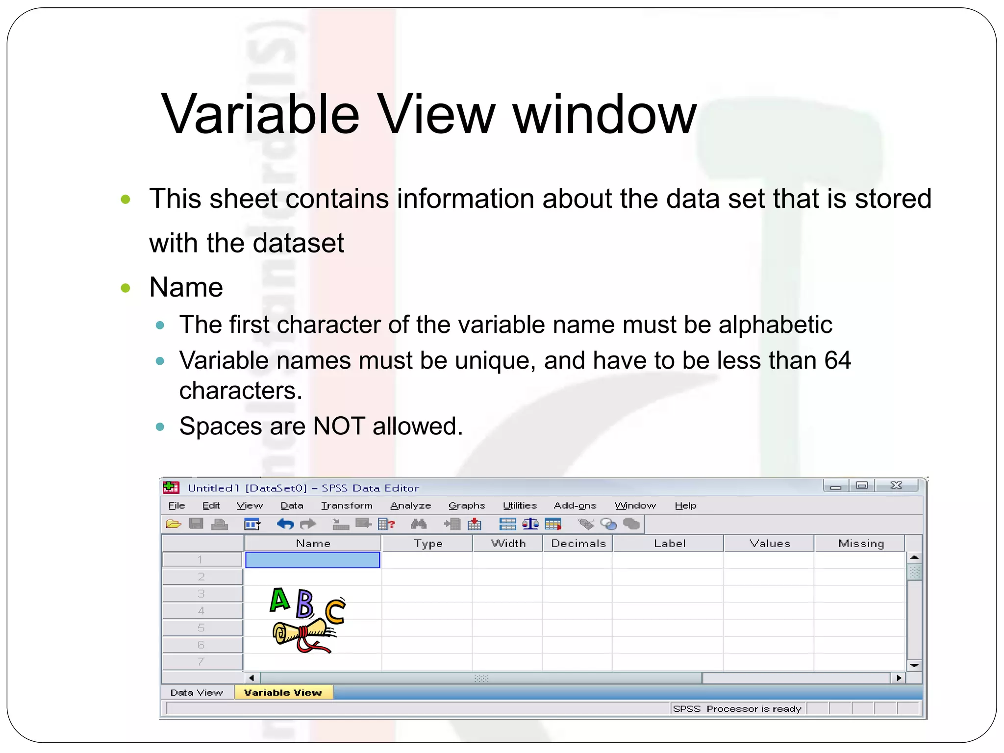
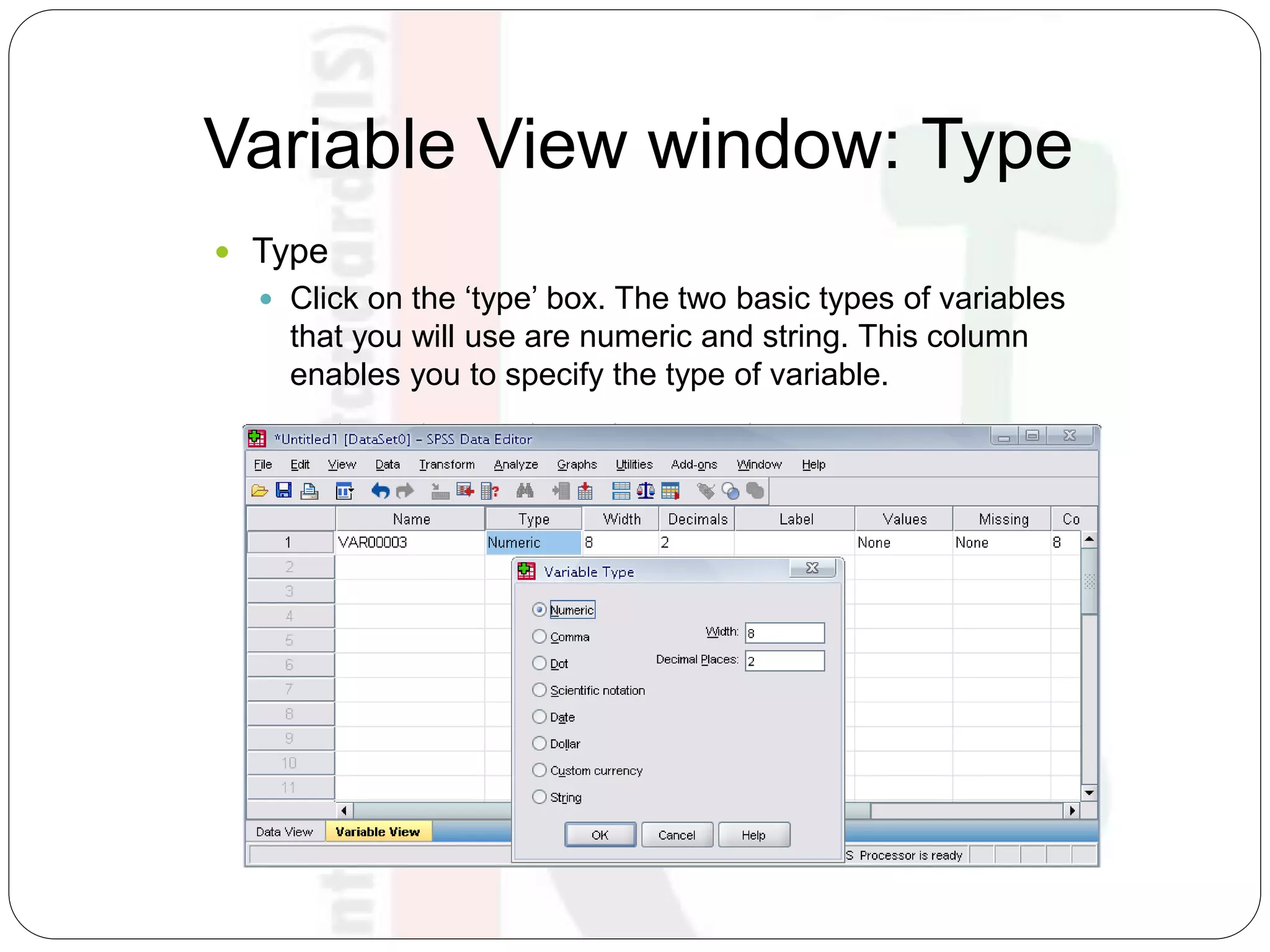
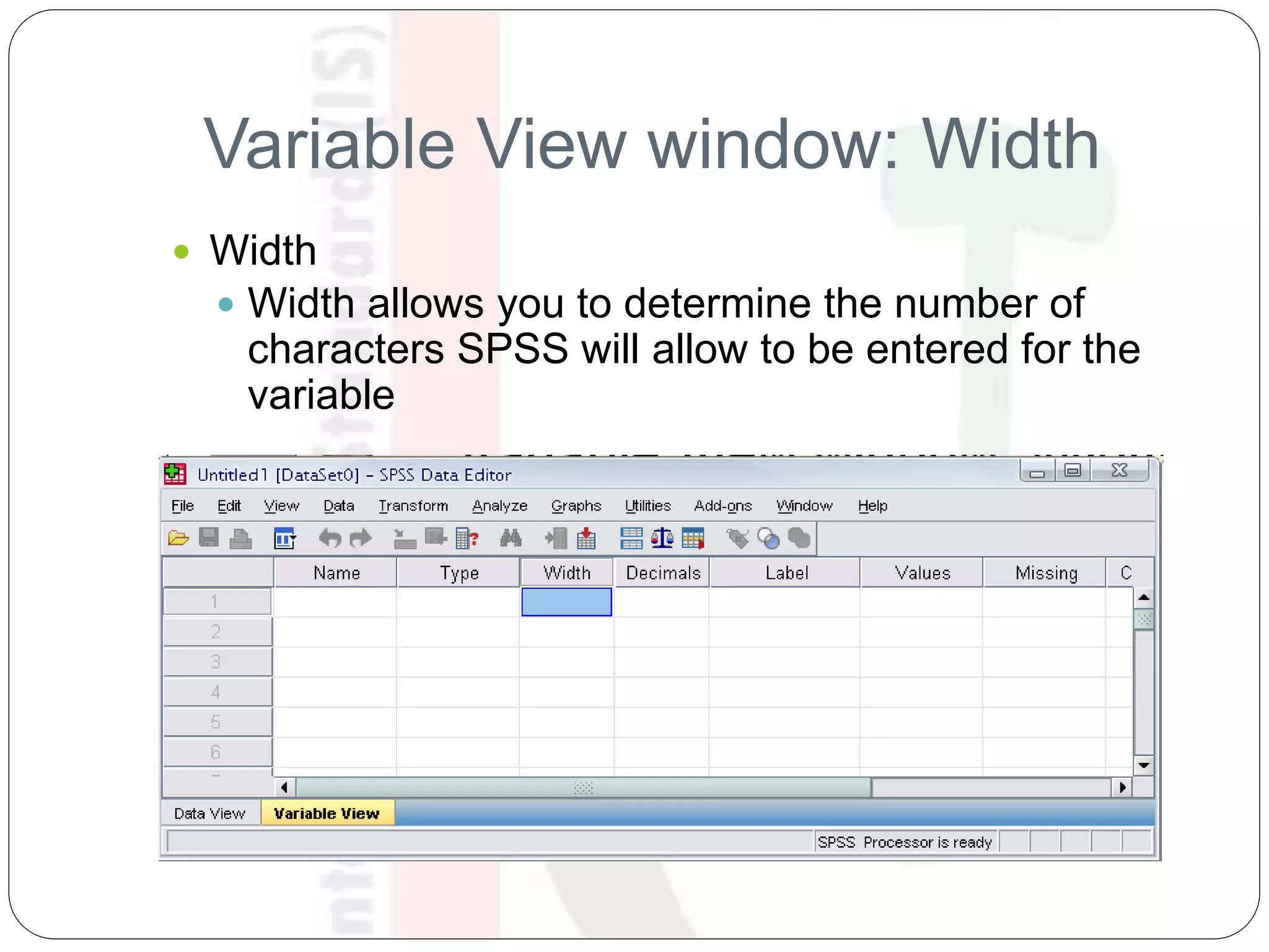
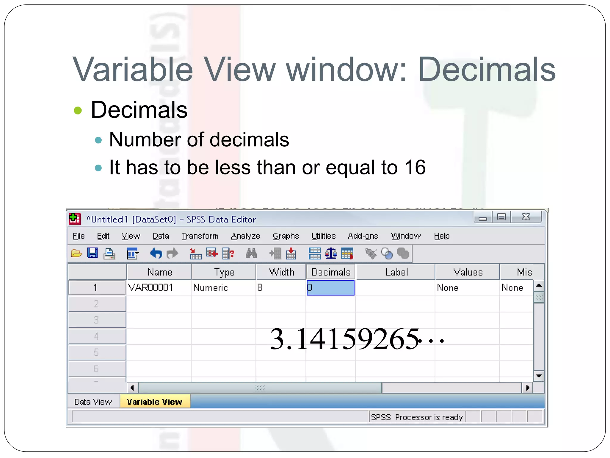
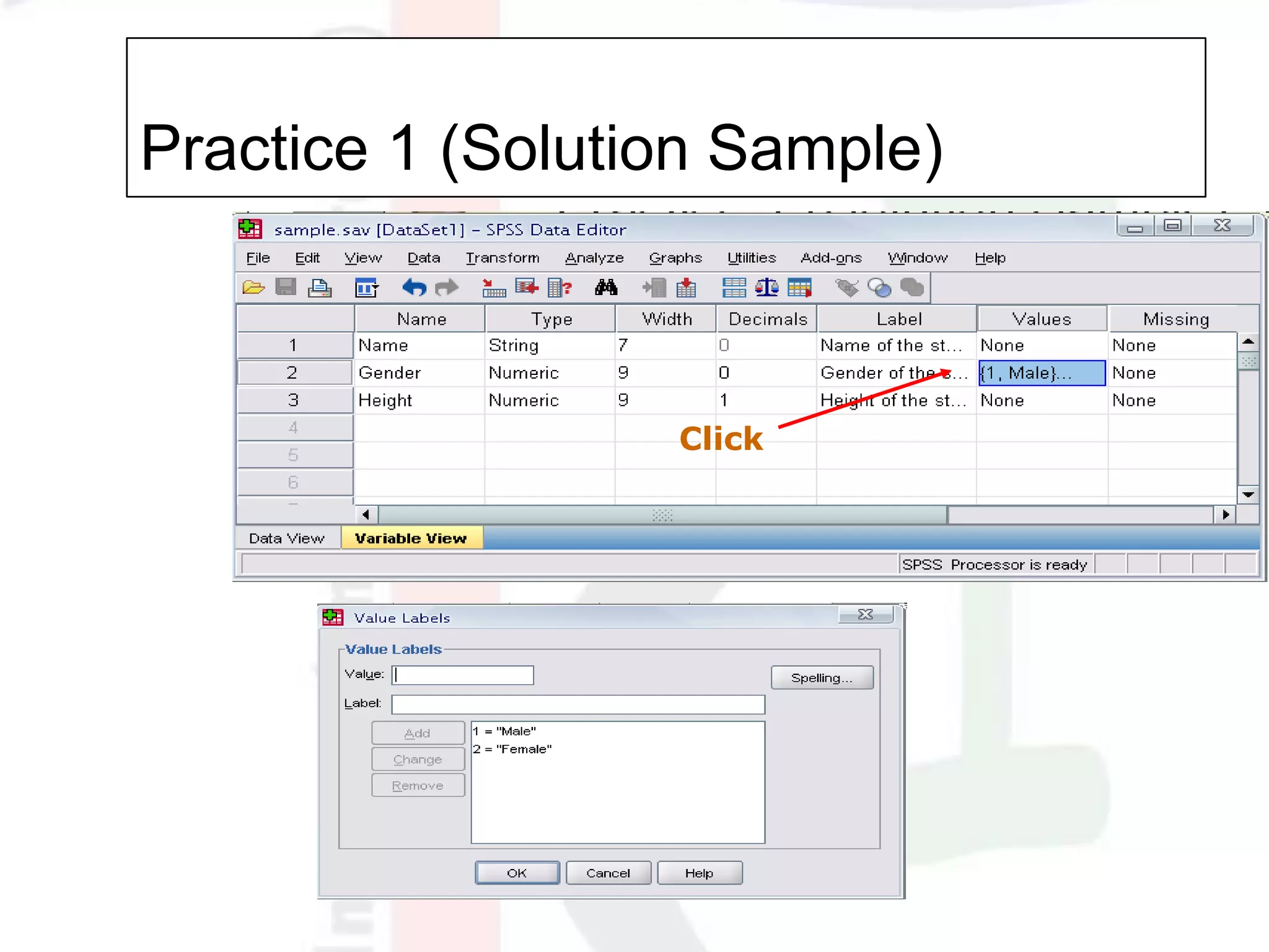
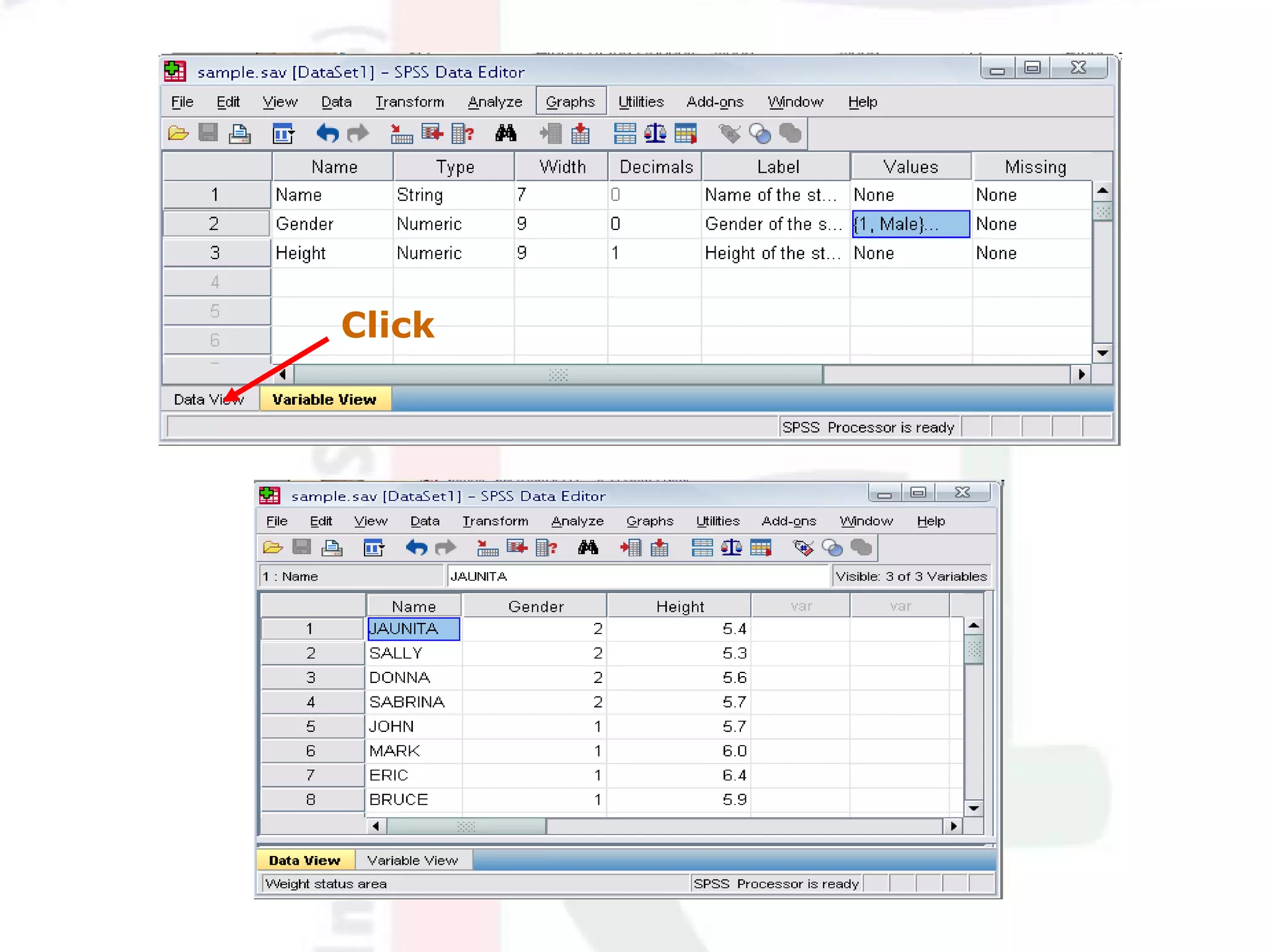
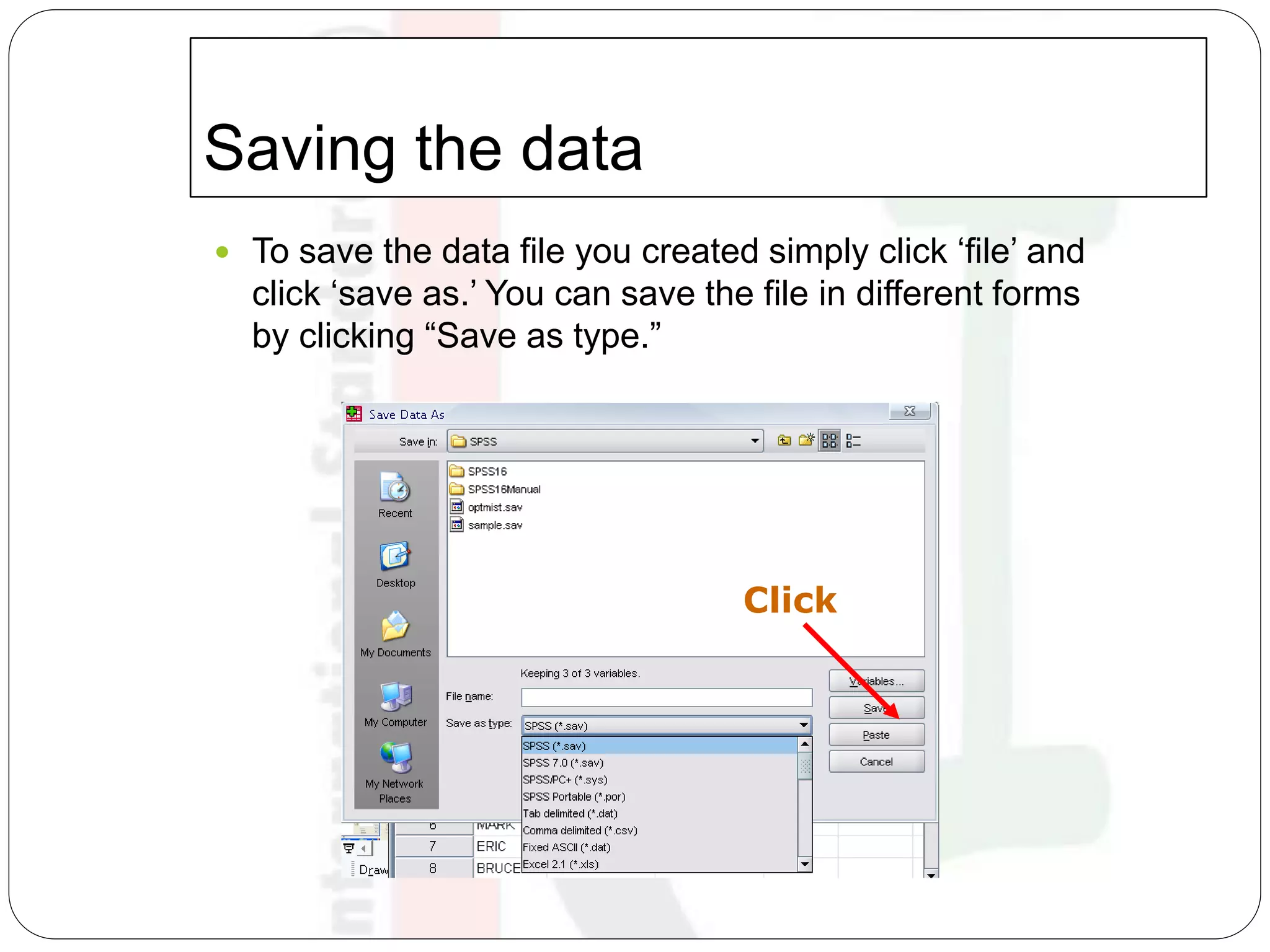
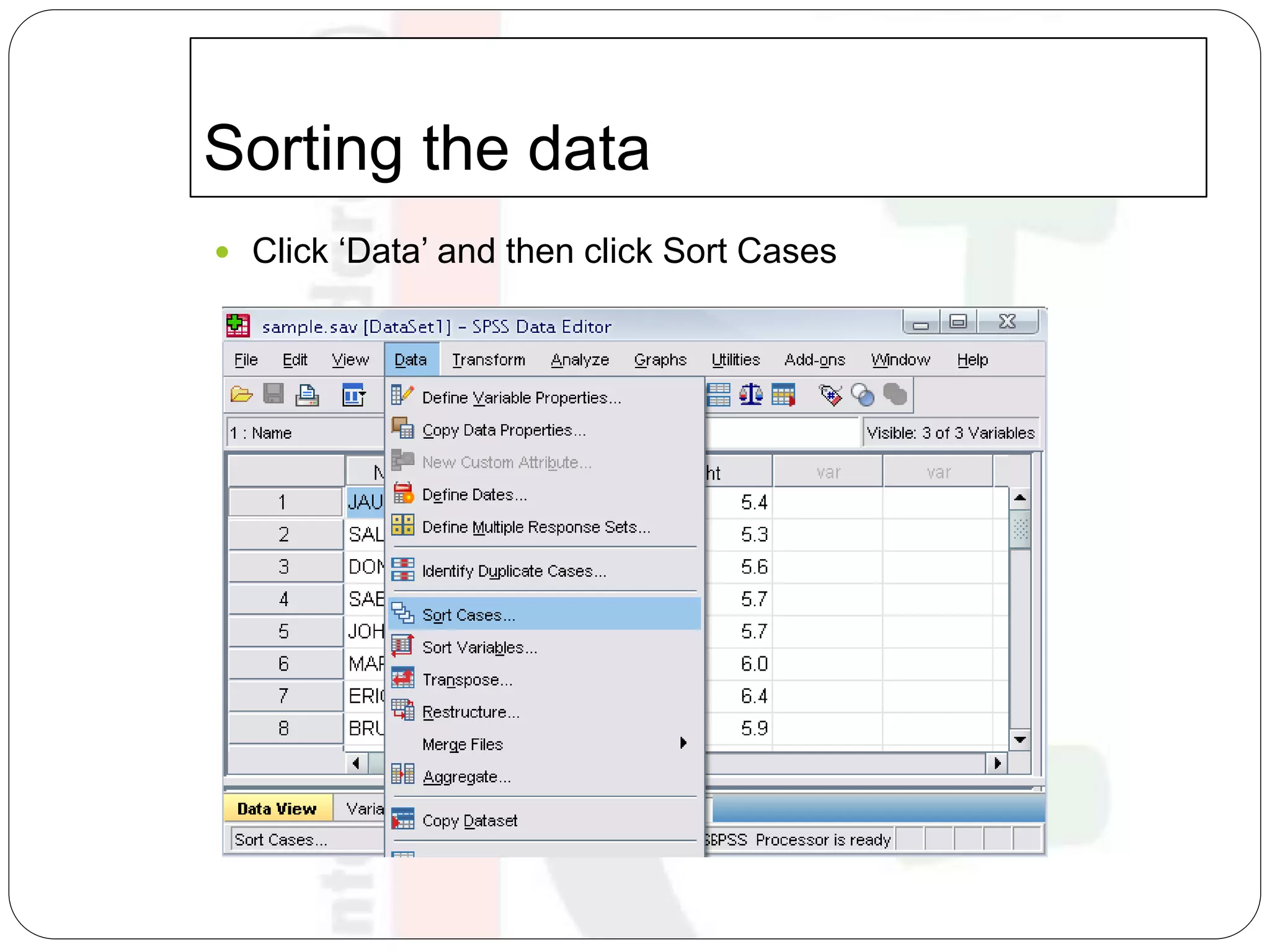
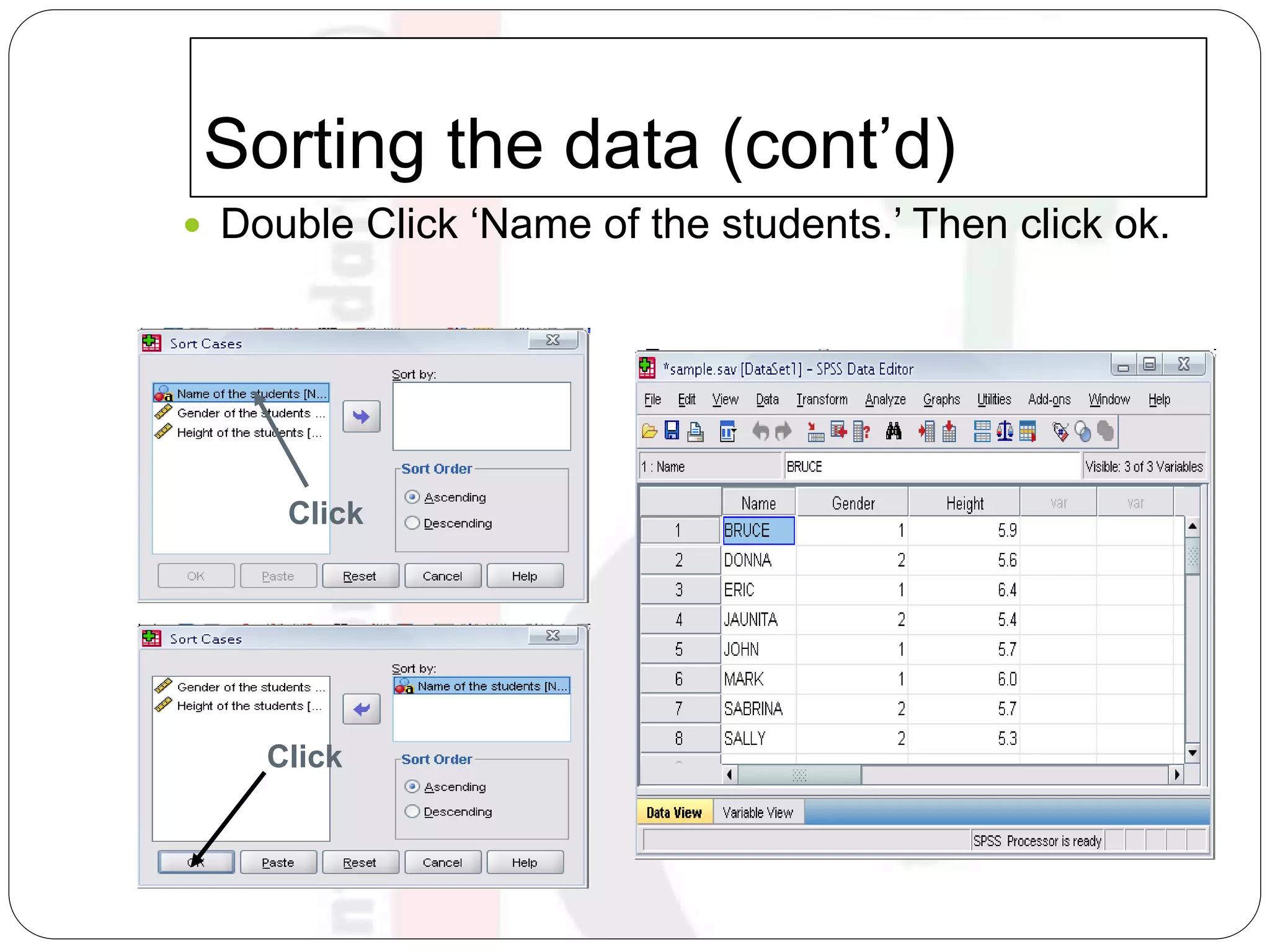
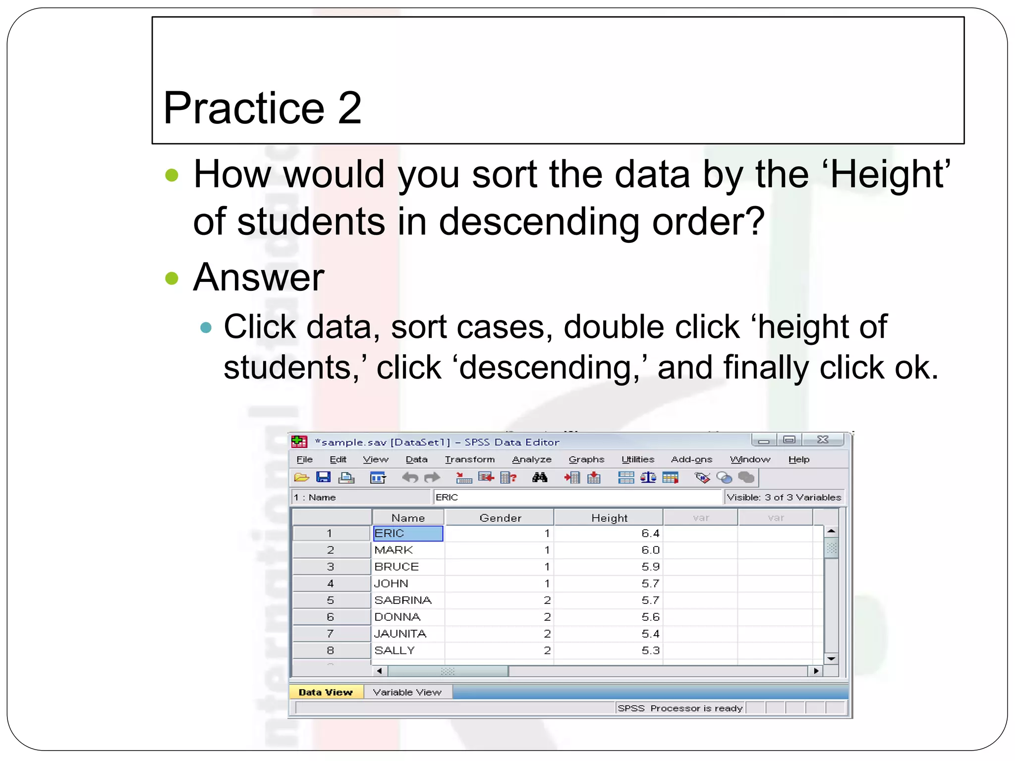
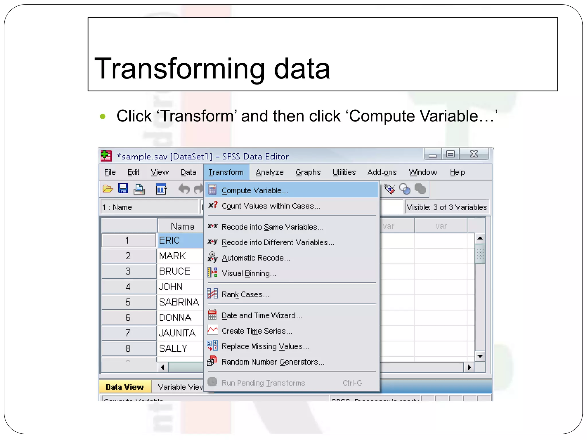
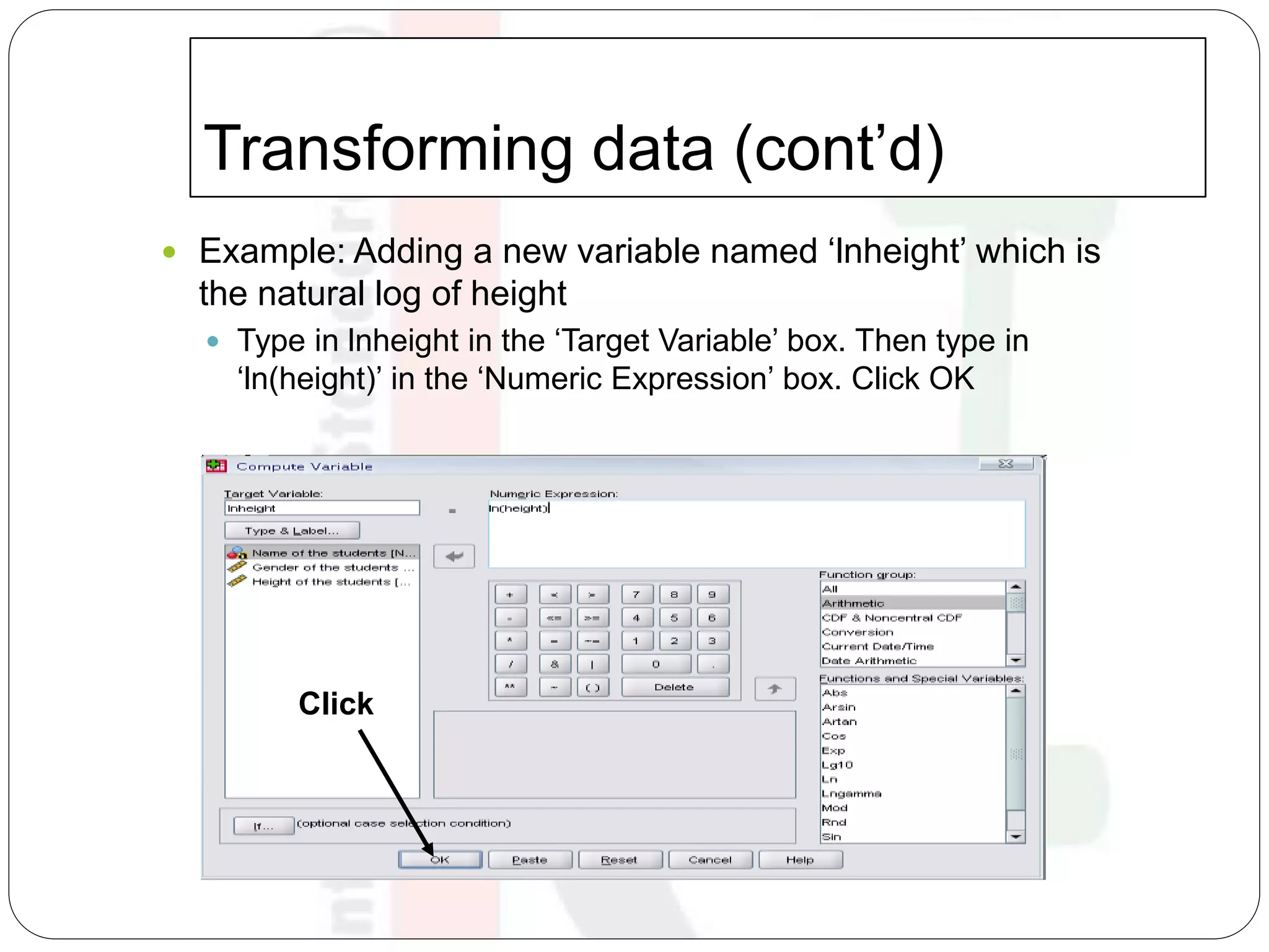
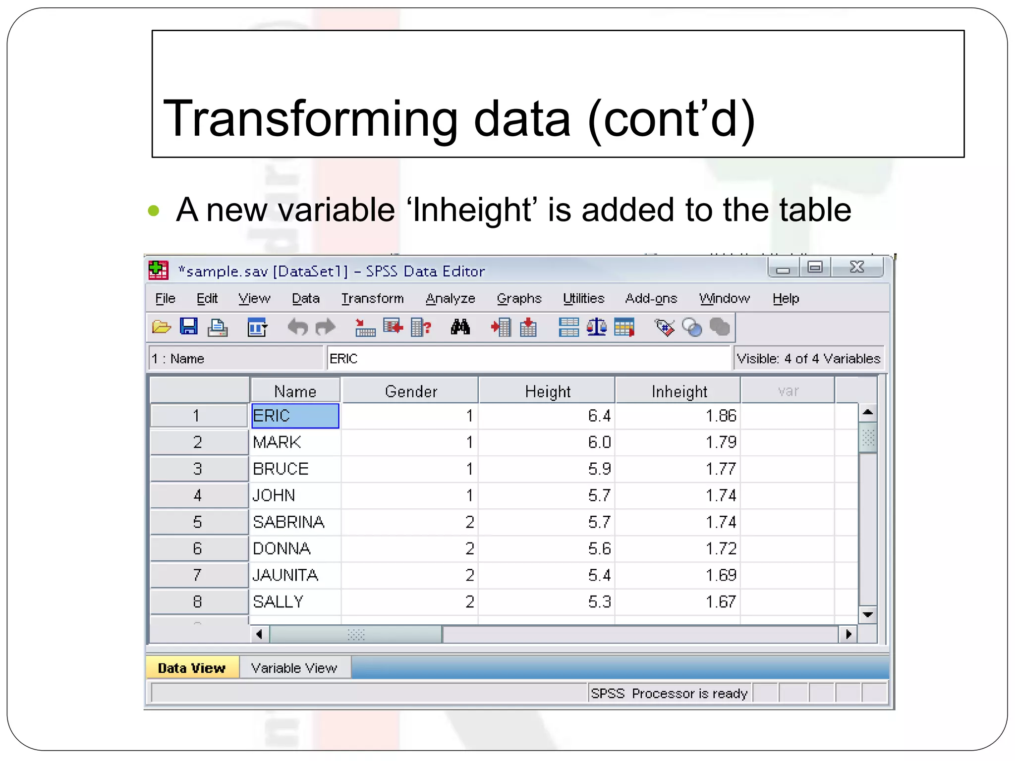
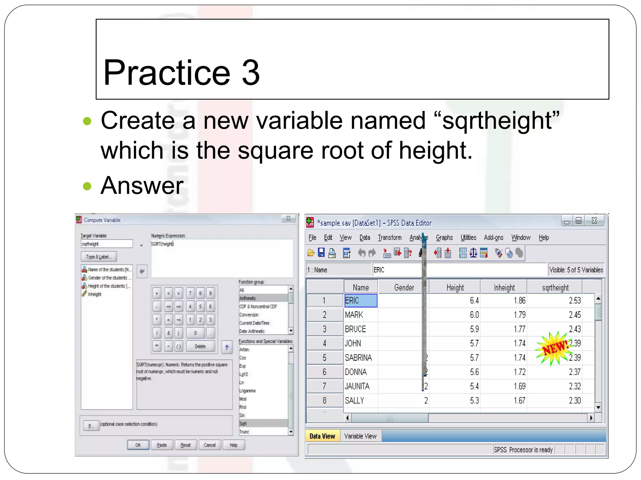
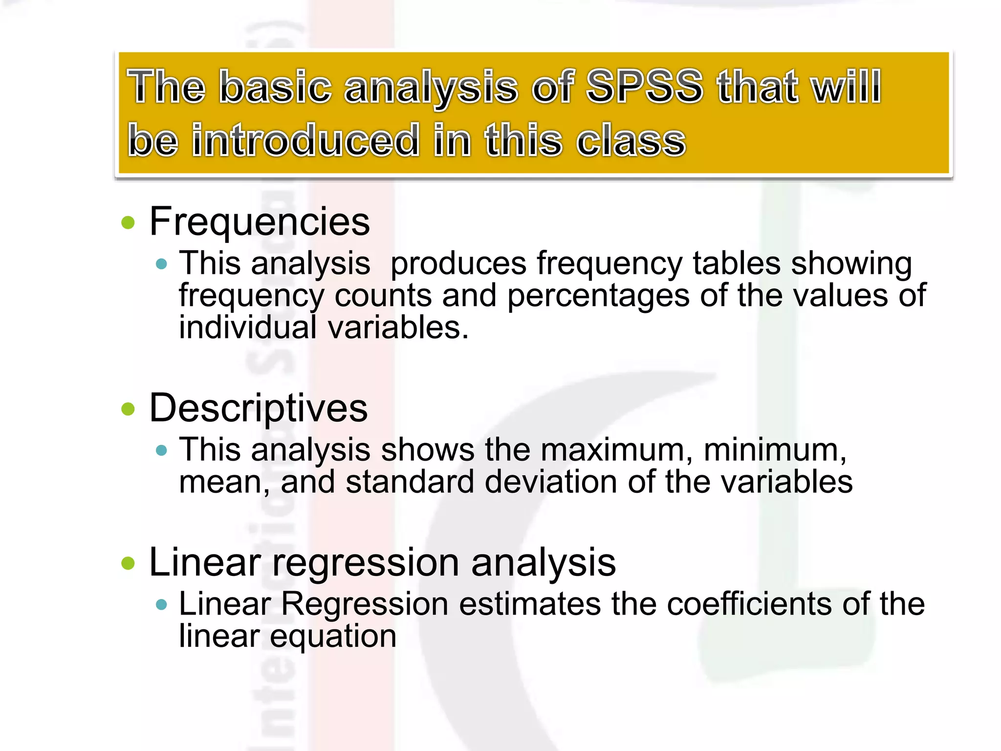
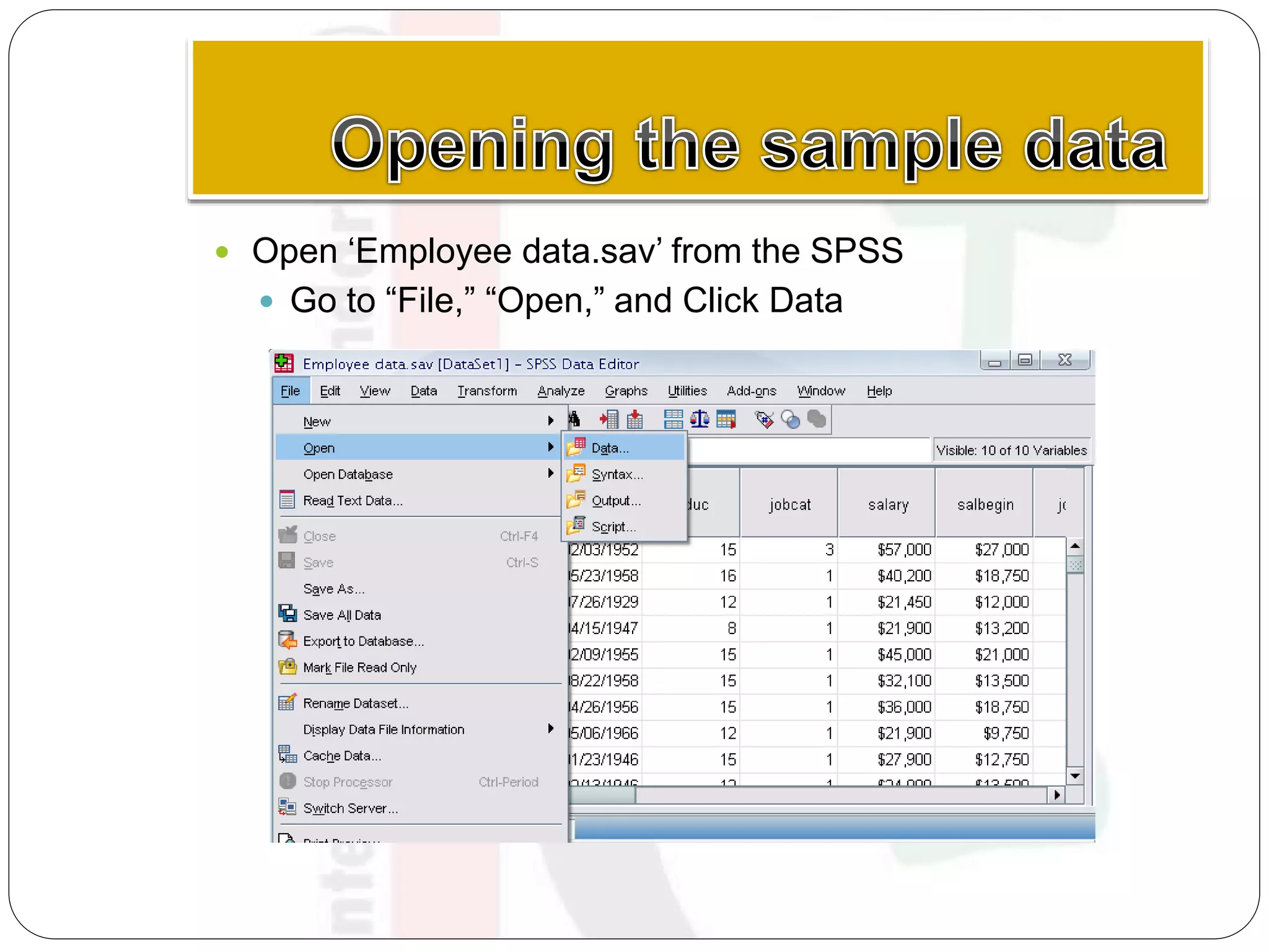
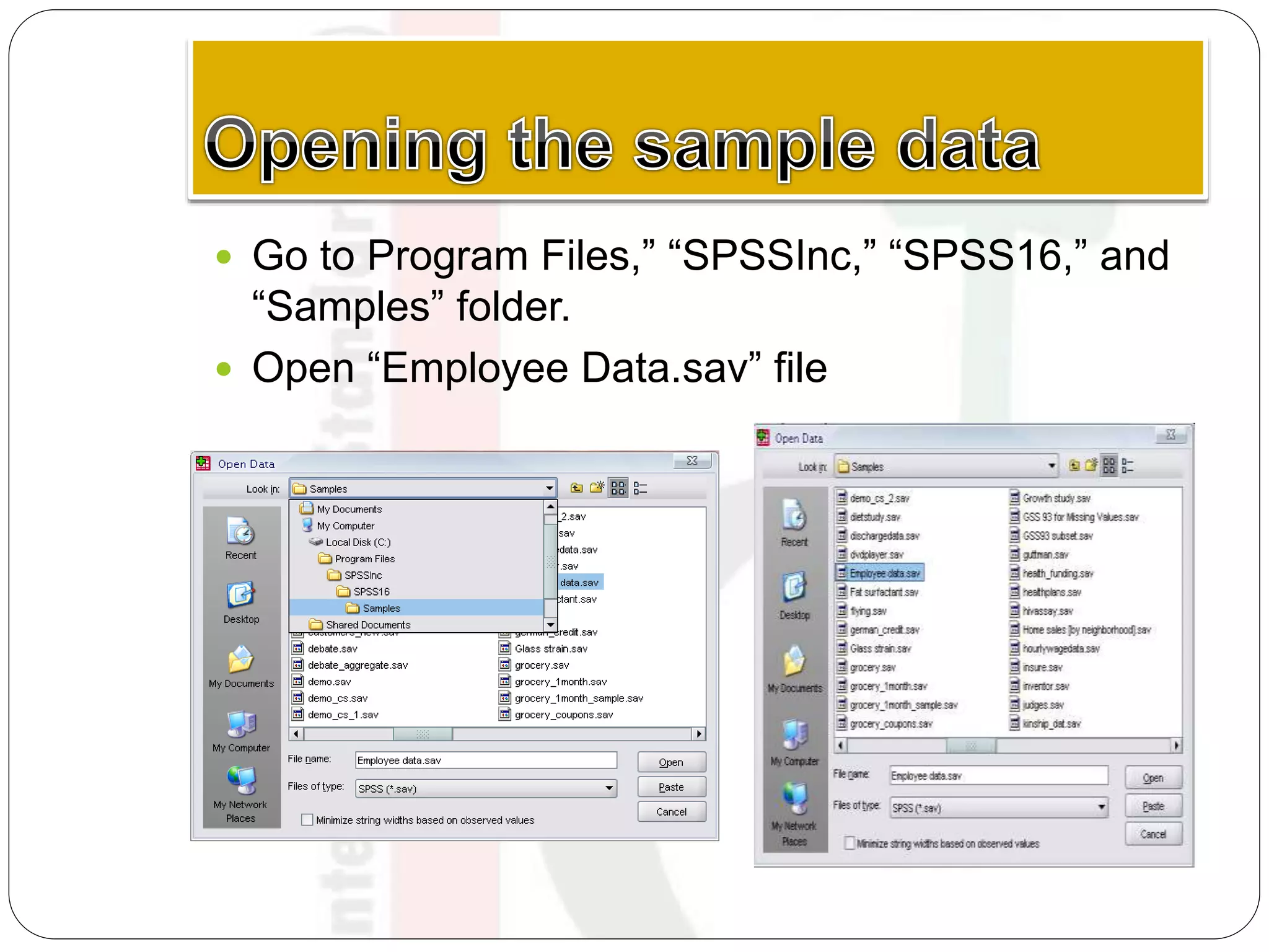
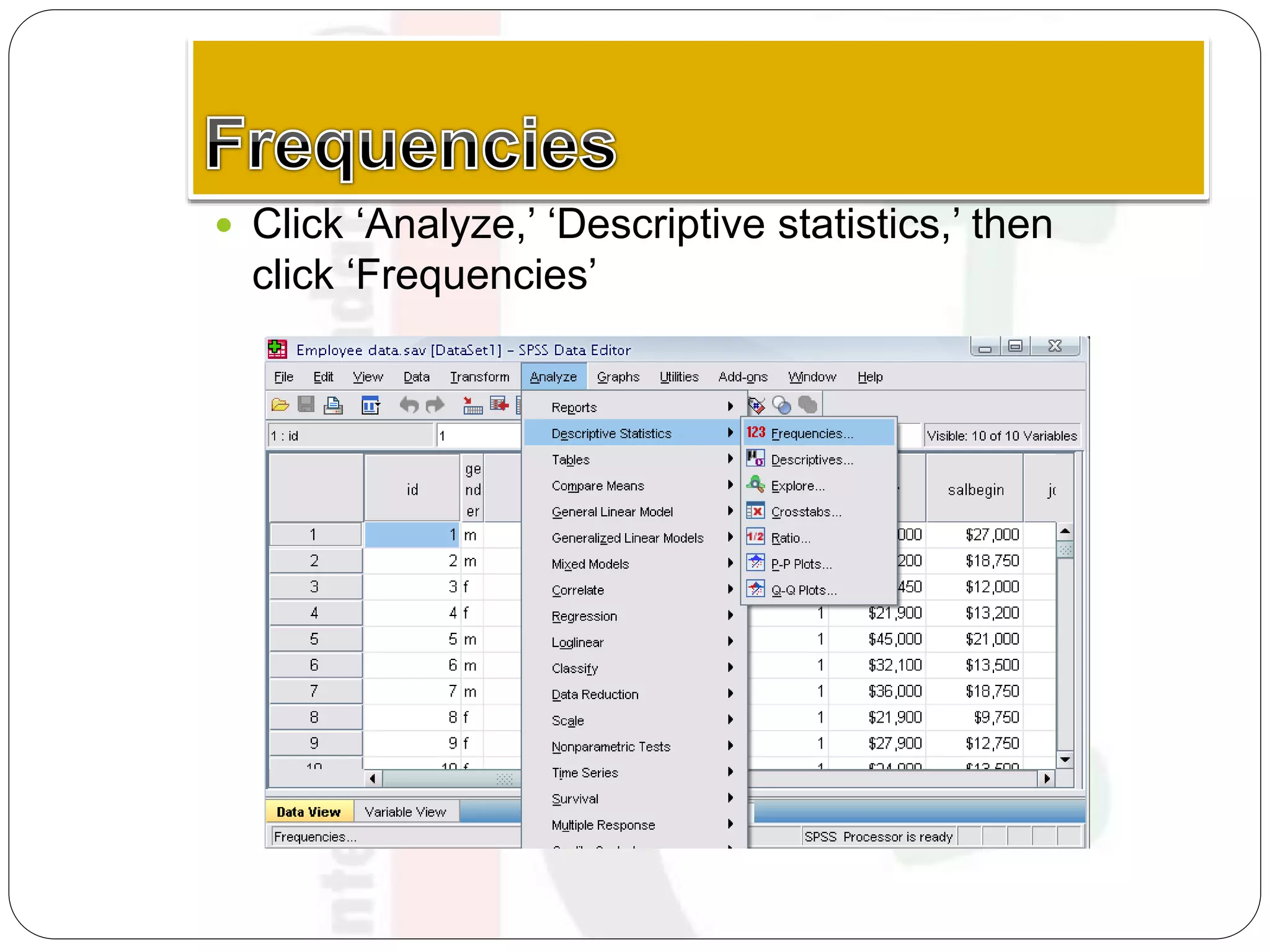
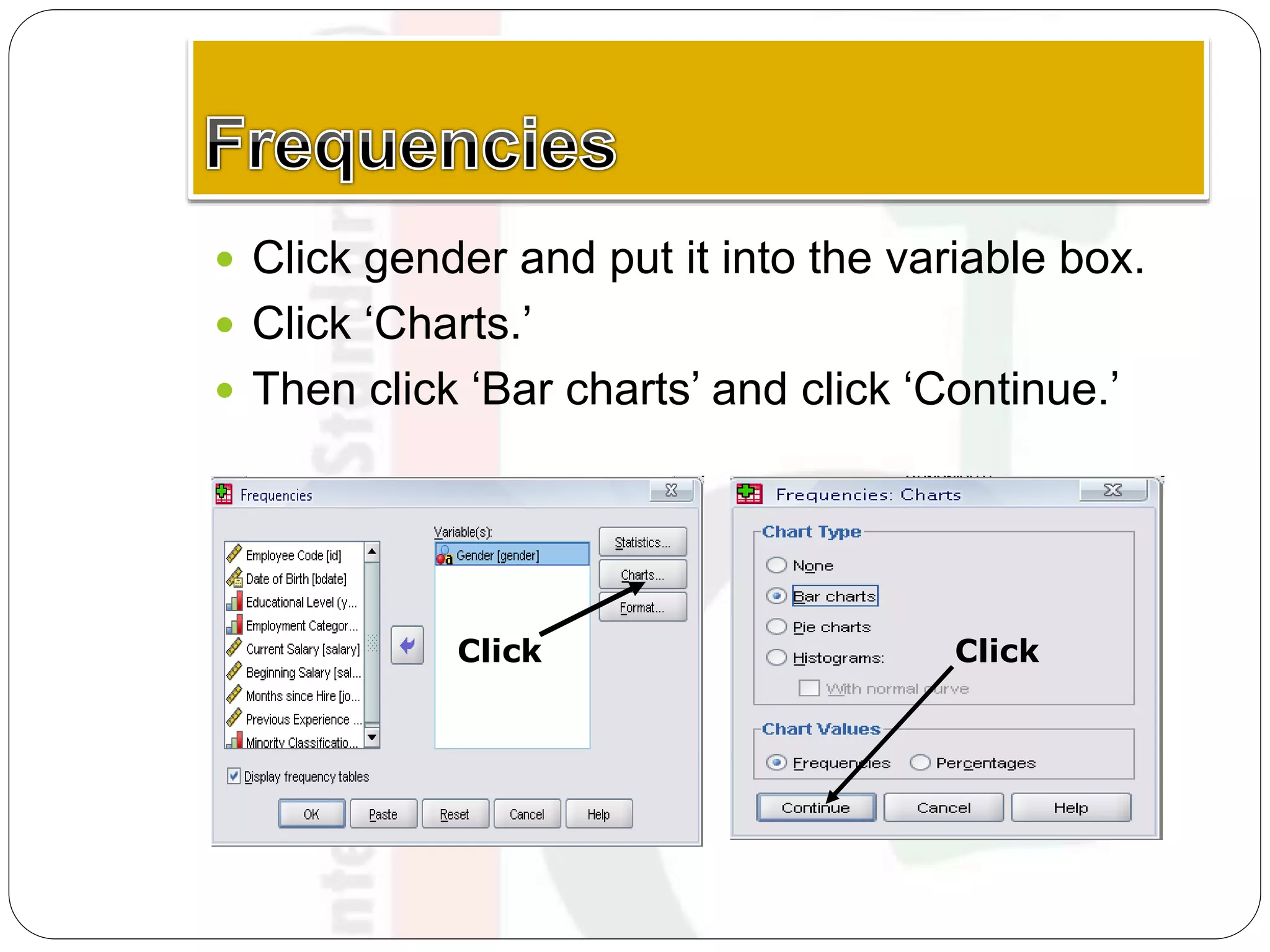
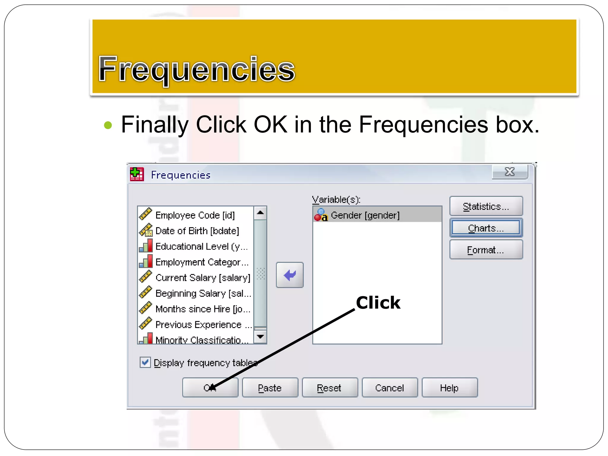
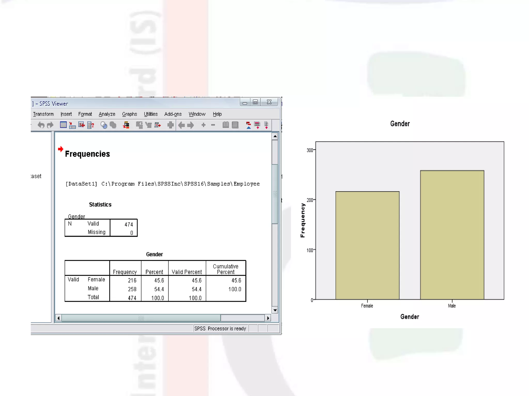
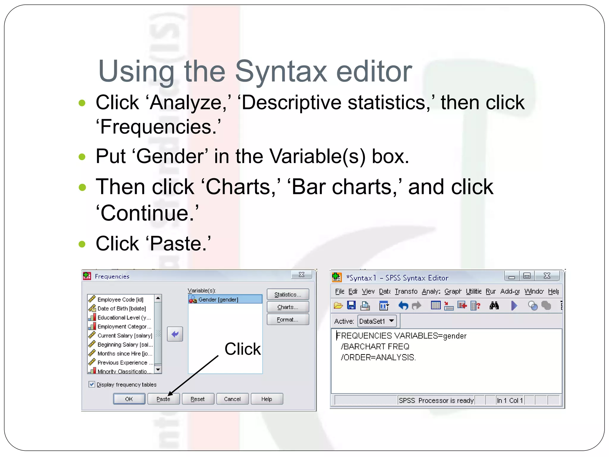
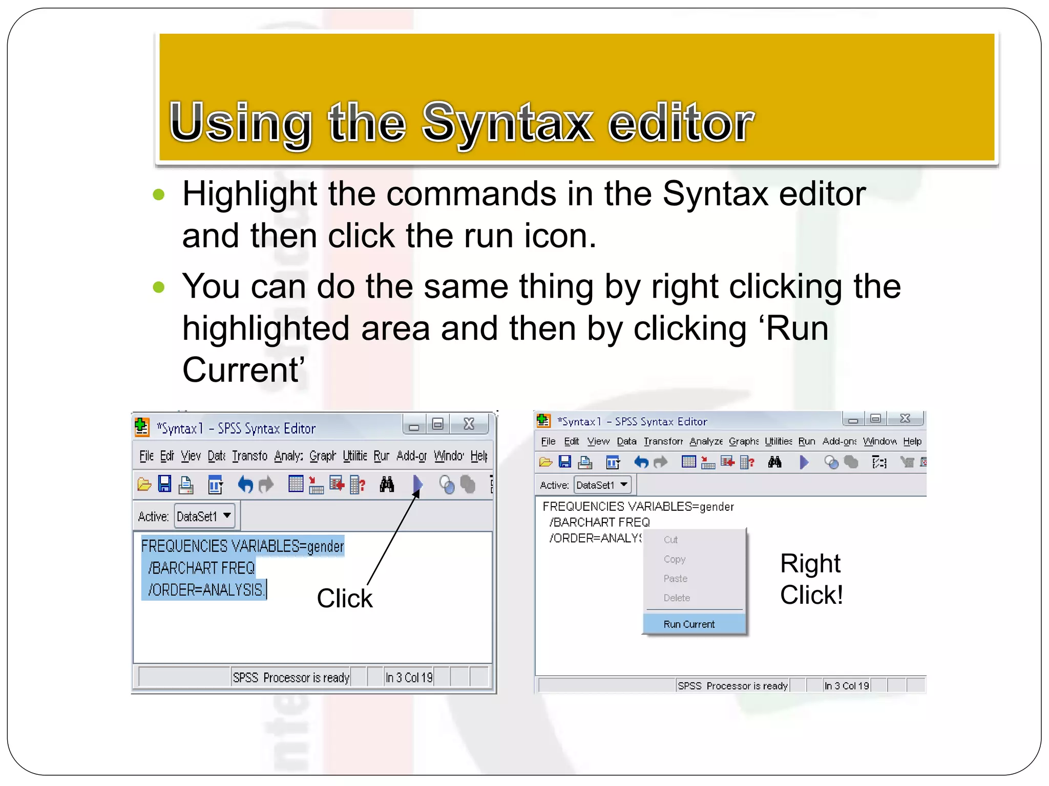
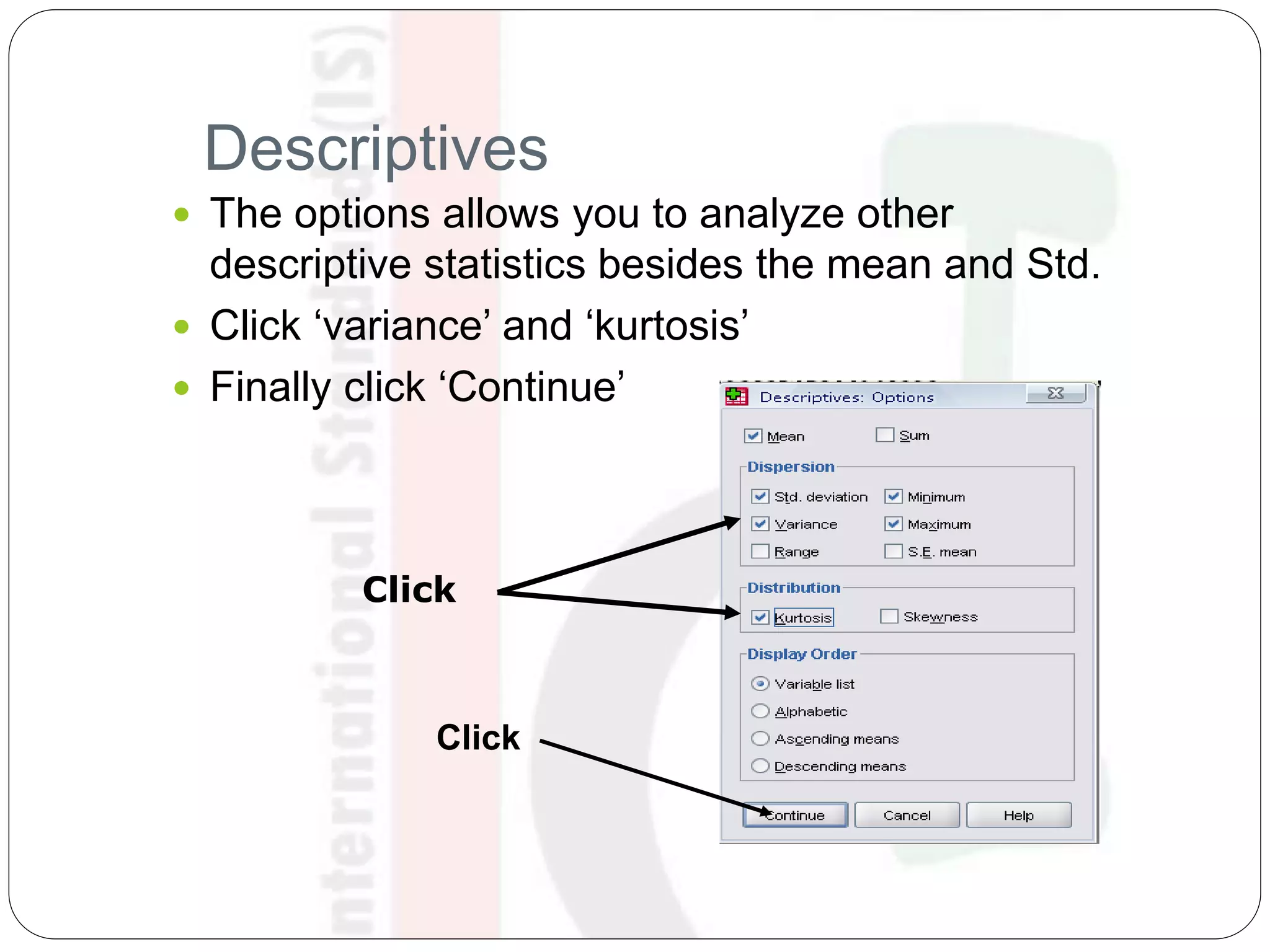
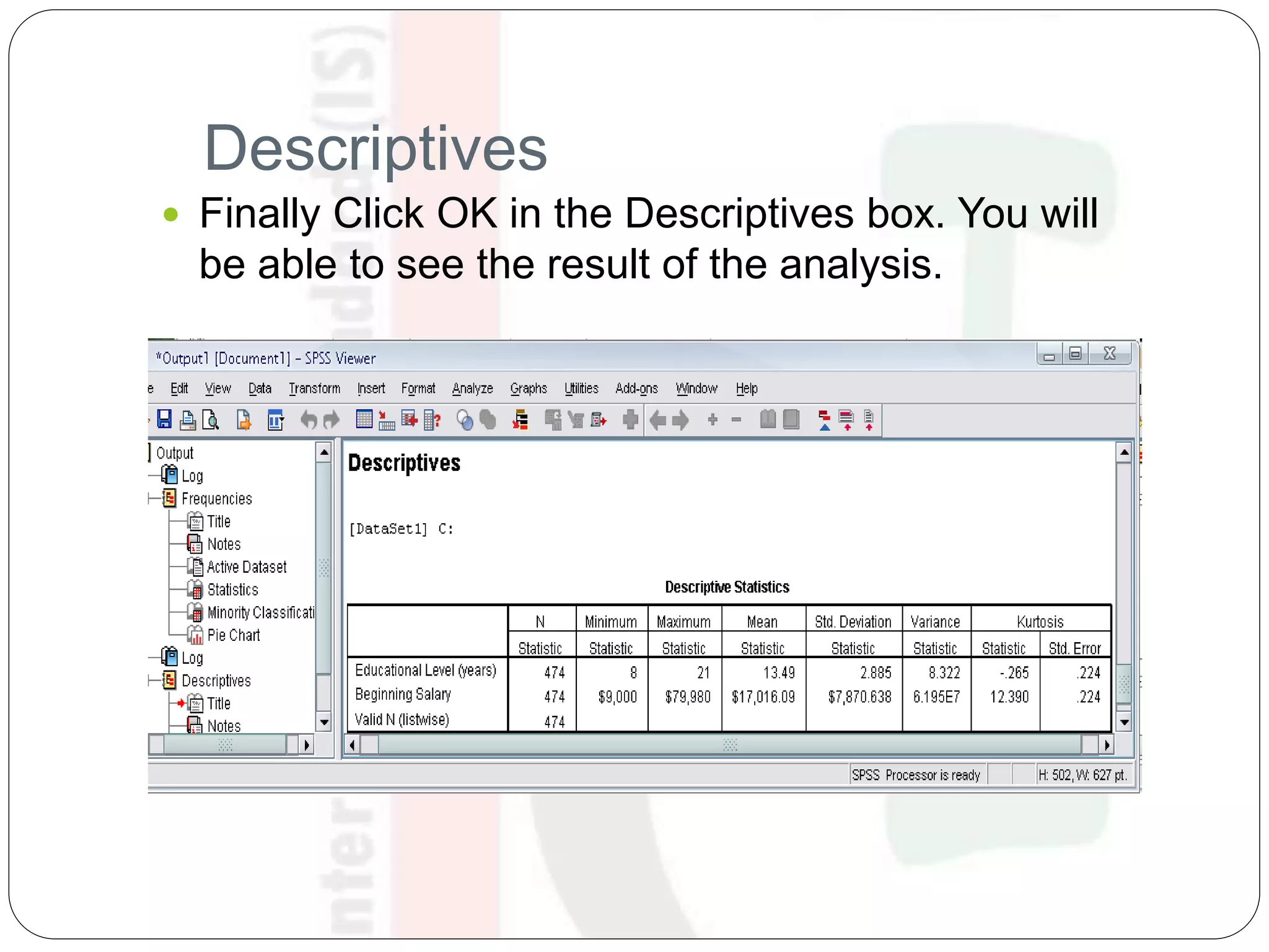
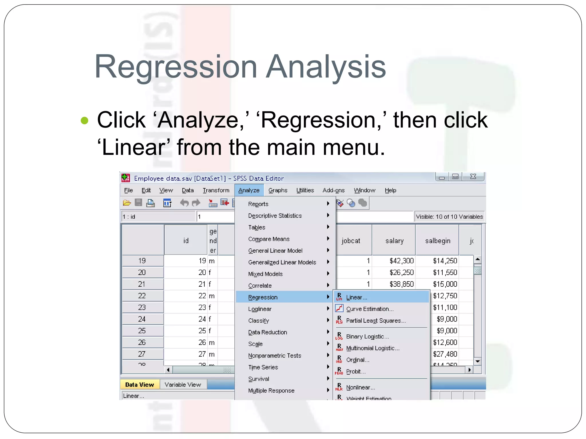
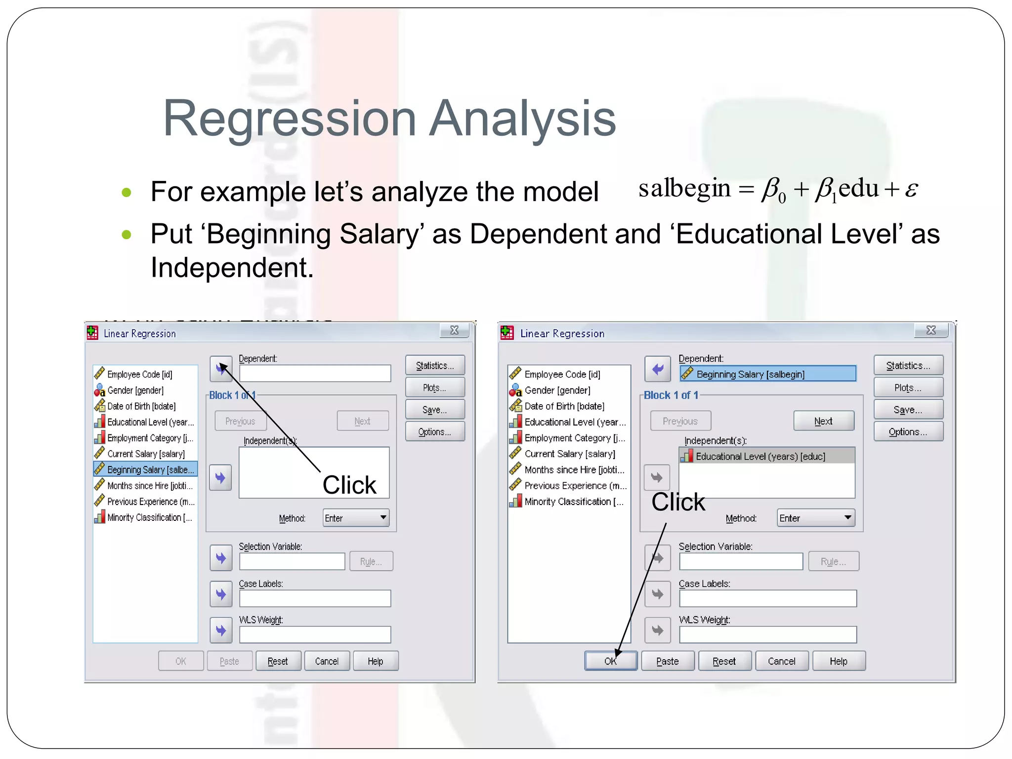
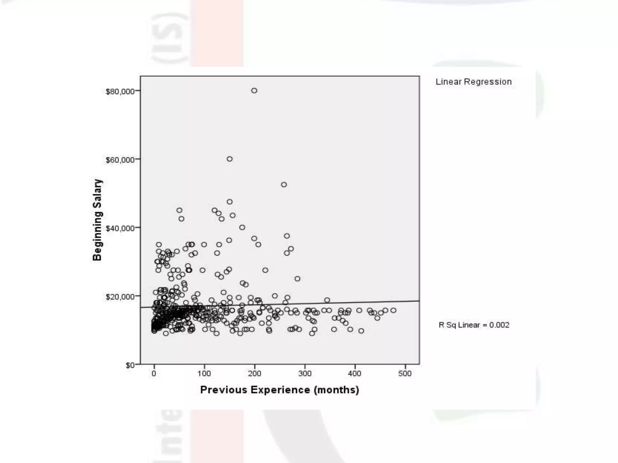


This document provides an introduction to SPSS, including descriptions of the four windows in SPSS, basics of managing data files, and basic analysis functions. It discusses the data editor, output viewer, syntax editor, and script windows. It covers opening SPSS, defining and managing variables, saving and sorting data, transforming variables through computations, and conducting basic analyses like frequencies, descriptives, and linear regression. Examples provided include creating new variables, sorting by height, and analyzing relationships between education level and starting salary.


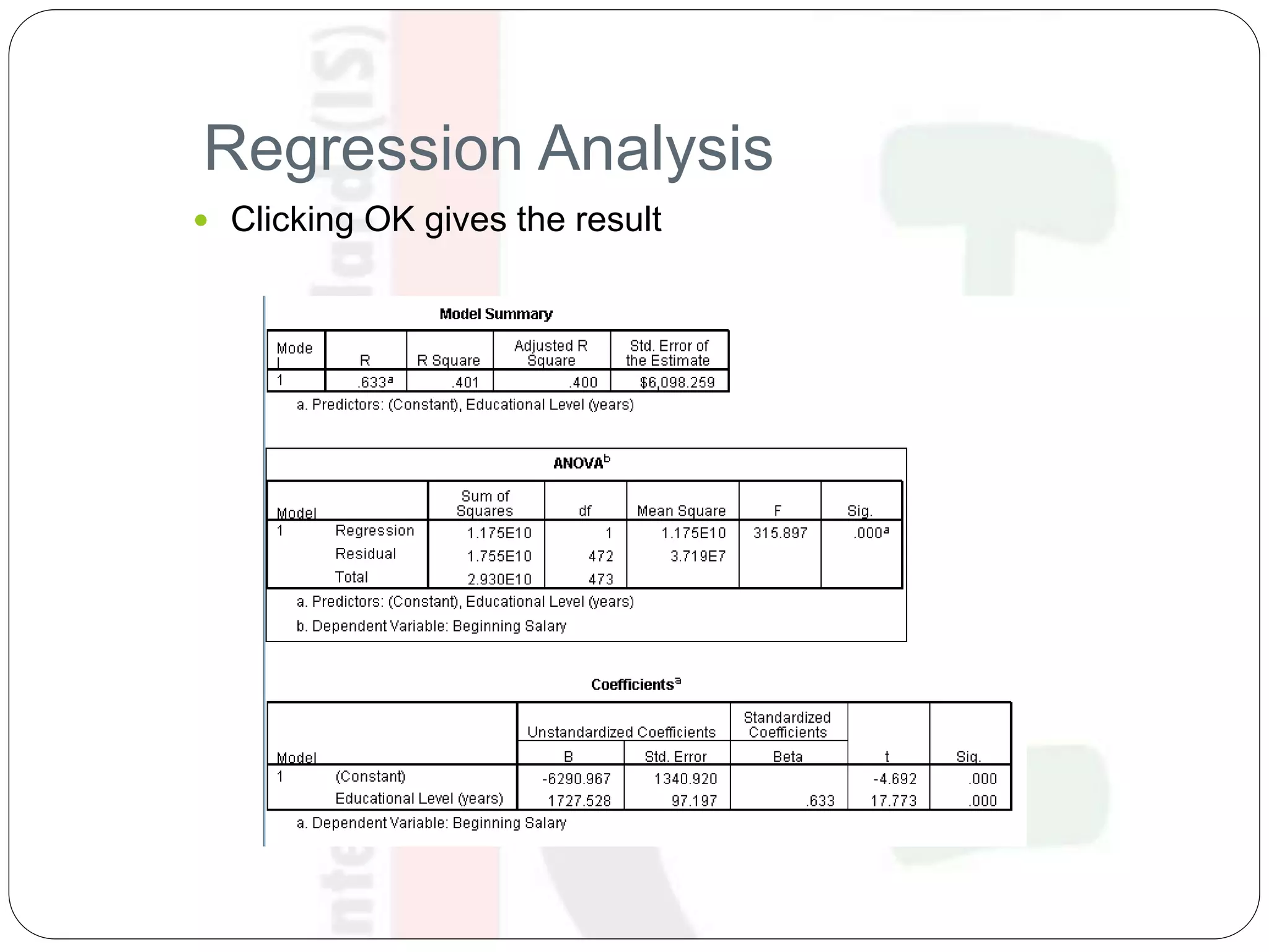
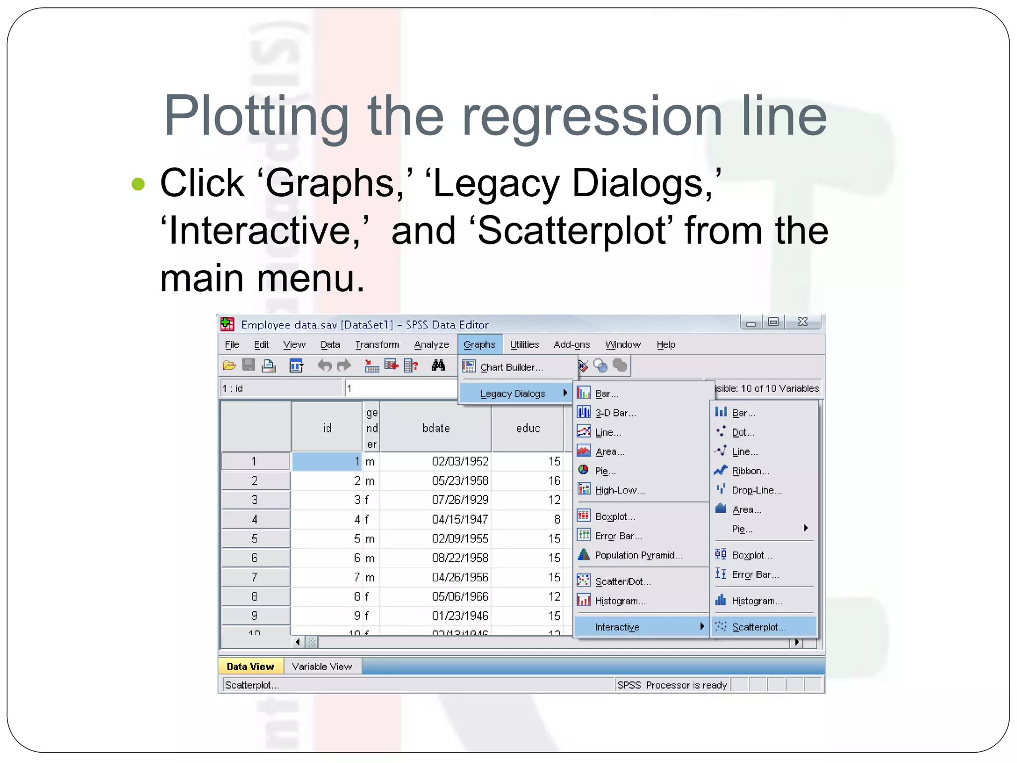
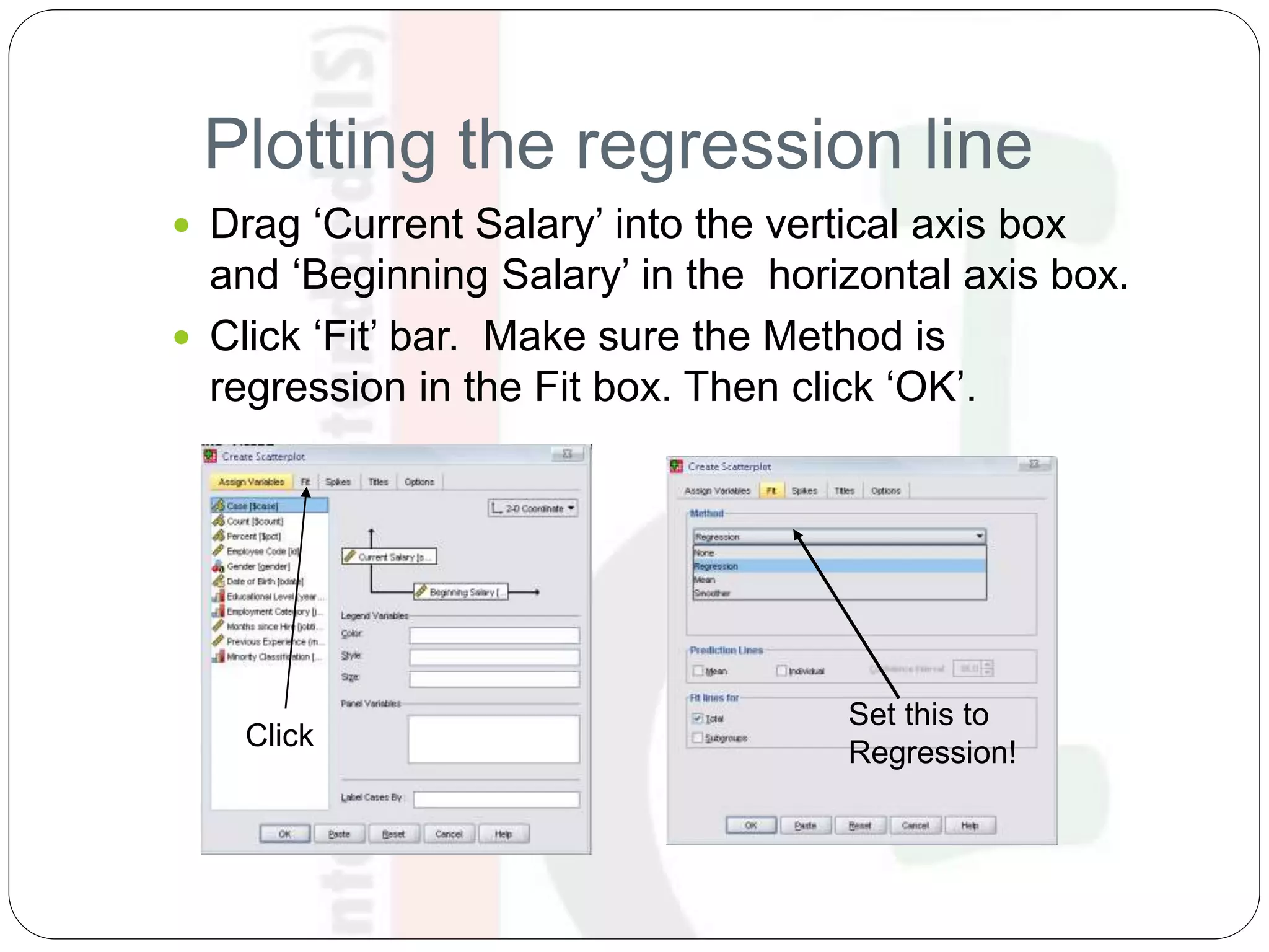
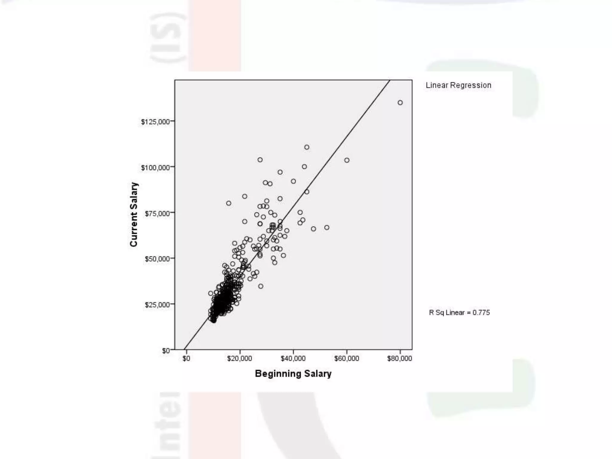
![SPSS Lecture_1 [Autosaved].pptx](https://cdn.slidesharecdn.com/ss_thumbnails/spsslecture1autosaved-231105165336-b29c7b18-thumbnail.jpg?width=640&height=640&fit=bounds)

