This presentation contain almost everything about the algorithms- its definition, designing, complexity analysis, running time calculations, common sorting and searching algorithms with their running time and examples.

1. 1Ramakant Soni, Asst. Professor, CS Dept., BKBIET Pilani
Ramakant Soni
Assistant Professor
CS Dept., BKBIET Pilani
ramakant.soni1988@gmail.com

2. What is an Algorithm ?
It is a step by step procedure or a set of steps to accomplish a task.
“An algorithm is any well-defined computational procedure that takes some value, or set of
values, as input and produces some value, or set of values as output."
Introduction to Algorithms by Thomas H. Cormen, Charles E. Leiserson, Ronald L. Rivest, Clifford Stein
Source: www.akashiclabs.com
2Ramakant Soni, Asst. Professor, CS Dept., BKBIET Pilani

3. Were do we use them?
 To find the best path to travel (Google Maps).
 For weather forecasting.
 To find structural patterns and cure diseases.
 For making games that can defeat us in it.(chess)
 For the processing done at the server each time we check the mail.
 When we take a selfie, edit them, post them to social media and get likes.
 To buy some products online and pay for it sitting at our home.
 For the synchronization in the traffic lights of the whole city.
 For software and techniques used to make animation movie.
 Even a simple program of adding, subtracting, multiplying is an algorithm and also calculating the speed, path, fuel of a
space shuttle is done by using algorithms.
 And many more……….(almost everywhere!)
3Ramakant Soni, Asst. Professor, CS Dept., BKBIET Pilani

4. Write algorithm
Compute Complexity
& Optimize
Code program
Changes/ Modifications
Source: openclassroom.stanford.edu

5. Algorithm Example: Algorithm to add two numbers entered by user.
Step 1: Start
Step 2: Declare variables num1, num2 and sum.
Step 3: Read values num1 and num2.
Step 4: Add num1 and num2 and assign the result to sum.
sum←num1+num2
Step 5: Display sum
Step 6: Stop
#include <stdio.h>
int main()
{
int firstNo, secondNo, sum;
printf ("Enter two integers: ");
// Two integers entered by user is stored using scanf() function
scanf("%d %d",&firstNo, &secondNo);
// sum of two numbers in stored in variable sum
sum = firstNo + secondNo;
// Displays sum
printf ("%d + %d = %d", firstNo, secondNo, sum);
return 0;
}
Enter two integers: 12 ,11 Sum=12 + 11 = 23
5Ramakant Soni, Asst. Professor, CS Dept., BKBIET Pilani

6. Algorithm to find largest among three numbers.
Step 1: Start
Step 2: Declare variables a, b and c.
Step 3: Read variables a, b and c.
Step 4: If a>b
If a>c
Display a is the largest number.
Else
Display c is the largest number.
Else
If b>c
Display b is the largest number.
Else
Display c is the largest number.
Step 5: Stop
#include <stdio.h>
int main()
{
double n1, n2, n3;
printf("Enter three numbers: ");
scanf("%lf %lf %lf", &n1, &n2, &n3);
if (n1>=n2)
{ if(n1>=n3)
printf ("%.2lf is the largest number.", n1);
else
printf ("%.2lf is the largest number.", n3);
}
else
{ if(n2>=n3)
printf ("%.2lf is the largest number.", n2);
else
printf ("%.2lf is the largest number.",n3);
}
return 0;
}
6Ramakant Soni, Asst. Professor, CS Dept., BKBIET Pilani

7. Step 1: Start
Step 2: Declare variables n, factorial and i.
Step 3: Initialize variables: factorial←1
i←1
Step 4: Read value of n
Step 5: Repeat the steps until i=n
factorial ← factorial*i
i←i+1
Step 6: Display factorial
Step 7: Stop
#include <stdio.h>
int main()
{
int n, i;
unsigned long long factorial = 1;
printf("Enter an integer: ");
scanf("%d",&n);
// show error if the user enters a negative integer
if (n < 0)
printf("Error! Factorial of a negative number doesn't exist.");
else
{
for(i=1; i<=n; ++i)
{
factorial *= i; // factorial = factorial*i;
}
printf("Factorial of %d = %llu", n, factorial);
}
return 0;
}
Algorithm to find the factorial of a number entered by user.
Enter an integer: 10 Factorial of 10 = 10*9*8*7*6*5*4*3*2*1=3628800
7Ramakant Soni, Asst. Professor, CS Dept., BKBIET Pilani

8. Algorithm to find the Fibonacci series till term≤ n.
Step 1: Start
Step 2: Declare variables first_term, second_term and temp.
Step 3: Initialize variables first_term←0 second_term←1
Step 4: Display first_term and second_term
Step 5: Repeat the steps until second_term ≤ n
temp ← second_term
second_term ← second_term + first term
first_term ← temp
Display second_term
Step 6: Stop
#include <stdio.h>
int main()
{
int i, n, t1 = 0, t2 = 1, nextTerm = 0;
Printf ("Enter the number of terms: ");
Scanf ("%d",&n);
// displays the first two terms which is always 0 and 1
Printf ("Fibonacci Series: %d, %d, ", t1, t2);
// i = 3 because the first two terms are already displayed
for (i=3; i <= n; ++i)
{
nextTerm = t1 + t2;
t1 = t2;
t2 = nextTerm;
printf ("%d ", nextTerm);
}
return 0;
}
Enter a positive integer: 100 Fibonacci Series: 0, 1, 1, 2, 3, 5, 8, 13, 21, 34, 55, 89,
8Ramakant Soni, Asst. Professor, CS Dept., BKBIET Pilani

9. Algorithm Analysis
In computer science, the analysis of algorithms is the determination of the amount of resources (such as time
and storage) necessary to execute them.
The efficiency or running time of an algorithm is stated as a function relating the input length to the number
of steps (time complexity) or storage locations (space complexity).
1) Worst Case Analysis (Usually Done):In the worst case analysis, we calculate upper bound on running time of
an algorithm by considering worst case (a situation where algorithm takes maximum time)
2) Average Case Analysis (Sometimes done) :In average case analysis, we take all possible inputs and calculate
computing time for all of the inputs.
3) Best Case Analysis (Bogus) :In the best case analysis, we calculate lower bound on running time of an
algorithm.
Source: http://quiz.geeksforgeeks.org/lmns-algorithms/
9Ramakant Soni, Asst. Professor, CS Dept., BKBIET Pilani

10. Asymptotic Notations
• Θ Notation: The Theta notation bounds a functions from above and below, so it defines exact asymptotic behavior.
Θ((g(n)) = {f(n): there exist positive constants c1, c2 and n0 such that 0 <= c1*g(n) <= f(n) <= c2*g(n) for all n >= n0}
• Big O Notation: The Big O notation defines an upper bound of an algorithm, it bounds a function only from above.
O(g(n)) = { f(n): there exist positive constants c and n0 such that 0 <= f(n) <= cg(n) for all n >= n0}
• Ω Notation: The Omega notation provides an asymptotic lower bound.
Ω (g(n)) = {f(n): there exist positive constants c and n0 such that 0 <= cg(n) <= f(n) for all n >= n0}.
Source: http://quiz.geeksforgeeks.org/lmns-algorithms/
10Ramakant Soni, Asst. Professor, CS Dept., BKBIET Pilani

11. Big O Complexity Chart
Source: http://bigocheatsheet.com/
11Ramakant Soni, Asst. Professor, CS Dept., BKBIET Pilani

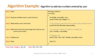
12. Insertion Sort
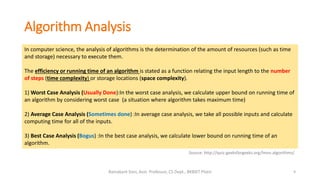
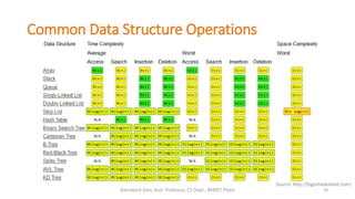
Statement Running Time of Each Step
InsertionSort (A, n) {
for i = 2 to n { c1n
key = A[i] c2(n-1)
j = i - 1; c3(n-1)
while (j > 0) and (A[j] > key) { c4T
A[j+1] = A[j] c5(T-(n-1))
j = j - 1 c6(T-(n-1))
} 0
A[j+1] = key c7(n-1)
} 0
}
T = t2 + t3 + … + tn where ti is number of while expression evaluations for the ith for loop iteration
12Ramakant Soni, Asst. Professor, CS Dept., BKBIET Pilani

13. Insertion Sort Example
13Ramakant Soni, Asst. Professor, CS Dept., BKBIET Pilani

14. Insertion Sort Analysis
• T(n) = c1n + c2(n-1) + c3(n-1) + c4T + c5(T - (n-1)) + c6(T - (n-1)) + c7(n-1) + c8T + c9n + c10
= = O(n2)
• What can T be?
• Best case -- inner loop body never executed- sorted elements
• ti = 1  T(n) is a linear function
• Worst case -- inner loop body executed for all previous elements
• ti = i  T(n) is a quadratic function
14Ramakant Soni, Asst. Professor, CS Dept., BKBIET Pilani

15. Merge Sort
MergeSort(A, left, right)
{
if (left < right)
{
mid = floor((left + right) / 2);
MergeSort (A, left, mid);
MergeSort (A, mid+1, right);
Merge(A, left, mid, right);
// Merge() takes two sorted subarrays of A and merges them into a single sorted subarray of A
}
}
When n ≥ 2, time for merge sort steps:
Divide : Just compute mid as the average of left and right, which takes constant time i.e. Θ(1).
Conquer : Recursively solve 2 sub-problems, each of size n/2, which is 2T(n/2).
Combine : MERGE on an n-element subarray takes Θ(n) time
15Ramakant Soni, Asst. Professor, CS Dept., BKBIET Pilani

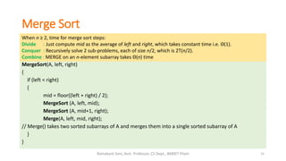
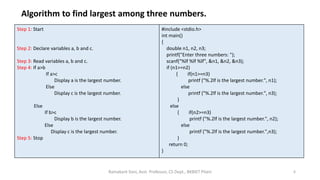
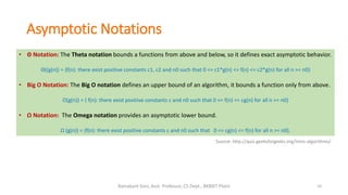
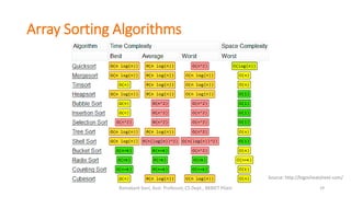
16. MERGE (A, left, mid, right )
1. n1 ← mid − left + 1
2. n2 ← right − mid
3. Create arrays L[1 . . n1 + 1] and R[1 . . n2 + 1]
4. FOR i ← 1 TO n1
5. DO L[i] ← A[left + i − 1]
6. FOR j ← 1 TO n2
7. DO R[j] ← A[mid + j ]
8. L[n1 + 1] ← ∞
9. R[n2 + 1] ← ∞
10. i ← 1
11. j ← 1
12. FOR k ← left TO right
13. DO IF L[i ] ≤ R[ j]
14. THEN A[k] ← L[i]
15. i ← i + 1
16. ELSE A[k] ← R[j]
17. j ← j + 1
Merge Sort
Source: http://www.personal.kent.edu
16Ramakant Soni, Asst. Professor, CS Dept., BKBIET Pilani

17. Analysis of Merge Sort
Statement Running Time of Each Step______
MergeSort (A, left, right) T(n)
{ if (left < right) (1)
{ mid = floor((left + right) / 2); (1)
MergeSort (A, left, mid); T(n/2)
MergeSort (A, mid+1, right); T(n/2)
Merge(A, left, mid, right); (n)
// Merge() takes two sorted subarrays of A and merges them into a single sorted subarray of A
}}
• So T(n) = (1) when n = 1, and
2T(n/2) + (n) when n > 1
Complexity= O(n log n)
17Ramakant Soni, Asst. Professor, CS Dept., BKBIET Pilani

18. The Master Theorem
• Given: a divide and conquer algorithm
• An algorithm that divides the problem of size n into a sub-problems, each of
size n/b
• Let the cost of each stage (i.e., the work to divide the problem + combine
solved sub-problems) be described by the function f(n)
• T(n) = a*T(n/b) + f(n)
18Ramakant Soni, Asst. Professor, CS Dept., BKBIET Pilani

19. The Master Theorem
if T(n) = a*T(n/b) + f(n) , then
 
 
 
 
 
 



































1
0
largefor)()/(
AND)(
)(
)(
)(
log)(
log
log
log
log
log
c
nncfbnaf
nnf
nnf
nOnf
nf
nn
n
nT
a
a
a
a
a
b
b
b
b
b



19Ramakant Soni, Asst. Professor, CS Dept., BKBIET Pilani

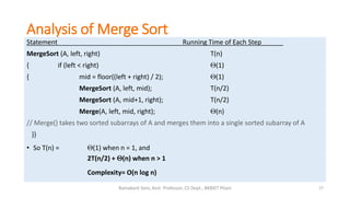
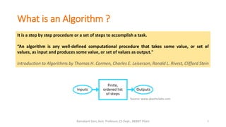
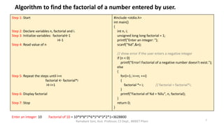
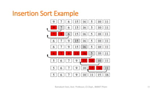
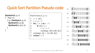
20. Quick Sort
Quicksort(A, p, r)
{ if (p < r)
{ q = Partition(A, p, r);
Quicksort(A, p, q);
Quicksort(A, q+1, r);
}
}
Another divide-and-conquer algorithm
• The array A[p .. r] is partitioned into two non-empty subarrays A[p .. q] and A[q+1 ..r]
Invariant: All elements in A[p .. q] are less than all elements in A[q+1..r]
• The subarrays are recursively sorted by calls to quicksort
Unlike merge sort, no combining step: two subarrays form an already-sorted array
Actions that takes place in the partition() function:
• Rearranges the subarray in place
• End result:
• Two subarrays
• All values in first subarray  all values in second
• Returns the index of the “pivot” element separating the two subarrays
20Ramakant Soni, Asst. Professor, CS Dept., BKBIET Pilani

21. Quick Sort Partition Pseudo code
21Ramakant Soni, Asst. Professor, CS Dept., BKBIET Pilani
Quicksort(A, p, r)
{ if (p < r)
{ q = Partition(A, p, r);
Quicksort(A, p, q);
Quicksort(A, q+1, r);
}
}

22. Quick Sort Example & Analysis
In the worst case ( unbalanced partition ):
T(1) = (1)
T(n) = T(n - 1) + (n)
Works out to
T(n) = (n2)
In the best case ( balanced partition ):
T(n) = 2T(n/2) + (n)
Works out to
T(n) = (n log n)
22Ramakant Soni, Asst. Professor, CS Dept., BKBIET Pilani

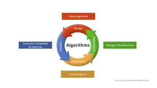
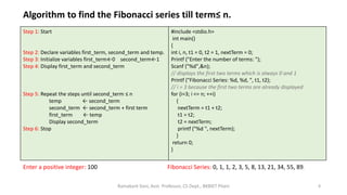
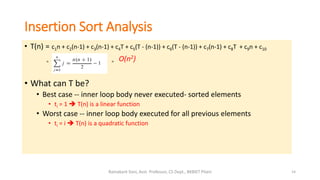
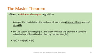
23. Linear Search
23Ramakant Soni, Asst. Professor, CS Dept., BKBIET Pilani
function find_Index (array, target)
{
for(var i = 0; i < array.length; ++i)
{
if (array[i] == target)
{
return i;
}
}
return -1;
}
• A linear search searches an element or value from an array till the
desired element or value is not found and it searches in a
sequence order.
• It compares the element with all the other elements given in the
list and if the element is matched it returns the value index else it
return -1.
• Running Time: T(n)= a(n-1) + b
Example: Search 5 in given data 5

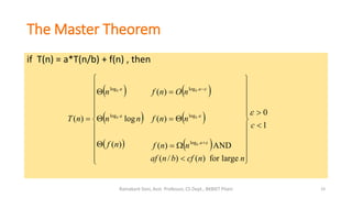
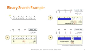
24. Binary Search
24Ramakant Soni, Asst. Professor, CS Dept., BKBIET Pilani
binary_search(A, low, high)
low = 1, high = size(A)
while low <= high
mid = floor(low + (high-low)/2)
if target == A[mid]
return mid
else if target < A[mid]
binary_search(A, low, mid-1)
else
binary_search(A, mid+1, high)
else
“target was not found”
Binary Search is an instance of divide-and-conquer paradigm.
Given an ordered array of n elements, the basic idea of binary search
is that for a given element we "probe" the middle element of the
array.
We continue in either the lower or upper segment of the array,
depending on the outcome of the probe until we reached the
required (given) element.
Complexity Analysis:
Binary Search can be accomplished in logarithmic time in the worst
case , i.e., T(n) = θ(log n).

25. Binary Search Example
25Ramakant Soni, Asst. Professor, CS Dept., BKBIET Pilani
1
2
3
Source: http://www.csit.parkland.edu

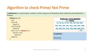
26. Algorithm to check Palindrome
26Ramakant Soni, Asst. Professor, CS Dept., BKBIET Pilani
A palindrome is a word, phrase, number, or other sequence of characters which reads the same backward or
forward.
function isPalindrome (text)
if text is null
return false
left ← 0
right ← text.length - 1
while (left < right)
if text[left] is not text[right]
return false
left ← left + 1
right ← right - 1
return true
Complexity:
The first function isPalindrome has a time
complexity of O(n/2) which is equal to O(n)
Palindrome Example:
CIVIC
LEVEL
RADAR
RACECAR
MOM

27. Algorithm to check Prime/ Not Prime
27Ramakant Soni, Asst. Professor, CS Dept., BKBIET Pilani
A palindrome is a word, phrase, number, or other sequence of characters which reads the same backward or
forward.
isPrime (int n){
int i;
if (n==2)
return 1;
if (n % 2==0)
return 0;
for (i = 3; i < =sqrt(n); i++)
if (n % I == 0)
return 0;
return 1;
}
Complexity:
O(sqrt(n)))

28. Common Data Structure Operations
Source: http://bigocheatsheet.com/
28Ramakant Soni, Asst. Professor, CS Dept., BKBIET Pilani

29. Array Sorting Algorithms
Source: http://bigocheatsheet.com/
29Ramakant Soni, Asst. Professor, CS Dept., BKBIET Pilani

30. All The Best !
30Ramakant Soni, Asst. Professor, CS Dept., BKBIET Pilani