Downloaded 1,080 times
![Pseudo-Code
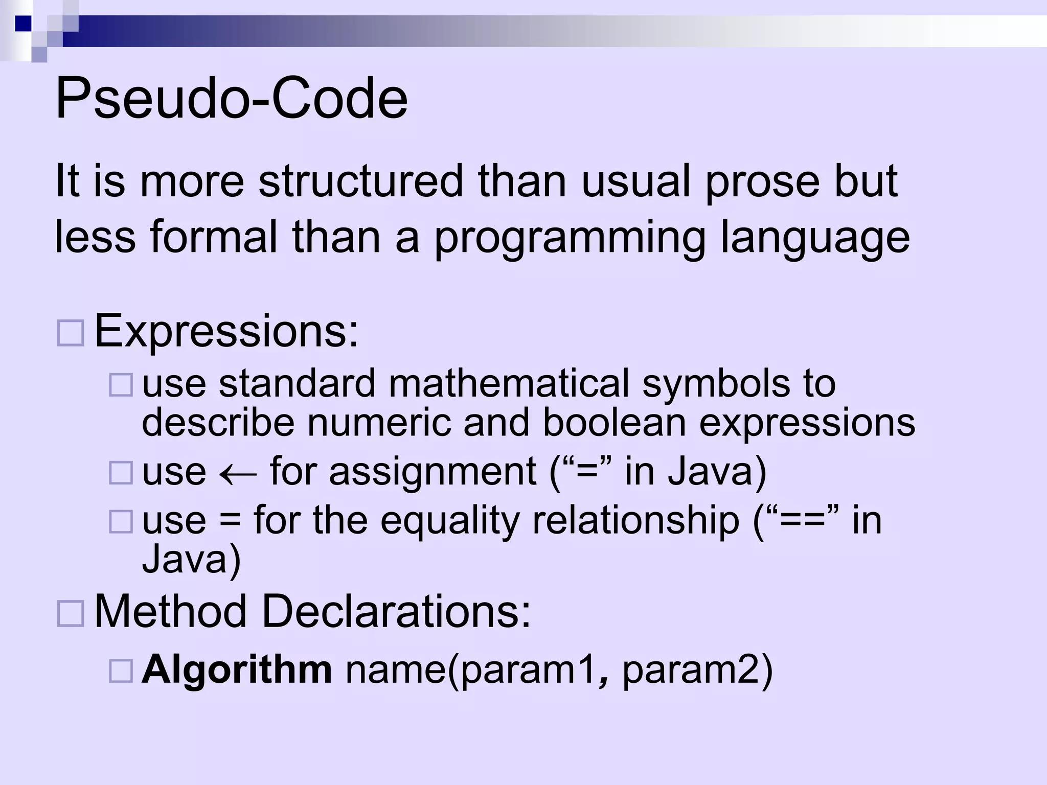
A mixture of natural language and high-level
programming concepts that describes the main
ideas behind a generic implementation of a data
structure or algorithm.
Eg: Algorithm arrayMax(A, n):
Input: An array A storing n integers.
Output: The maximum element in A.
currentMax A[0]
for i 1 to n-1 do
if currentMax < A[i] then currentMax A[i]
return currentMax](https://image.slidesharecdn.com/lec1-101217091247-phpapp02/75/Lec1-8-2048.jpg)
![Pseudo Code
Programming Constructs:
decision structures: if ... then ... [else ... ]
while-loops: while ... do
repeat-loops: repeat ... until ...
for-loop: for ... do
array indexing: A[i], A[i,j]
Methods:
calls:object method(args)
returns: return value](https://image.slidesharecdn.com/lec1-101217091247-phpapp02/75/Lec1-10-2048.jpg)
![Insertion Sort
A 3 4 6 8 9 7 2 5 1
1 j n
i
Strategy INPUT: A[1..n] – an array of integers
OUTPUT: a permutation of A such that
• Start “empty handed” A[1] A[2] … A[n]
• Insert a card in the right
position of the already sorted for j 2 to n do
hand key A[j]
• Continue until all cards are Insert A[j] into the sorted sequence
inserted/sorted A[1..j-1]
i j-1
while i>0 and A[i]>key
do A[i+1] A[i]
i--
A[i+1] key](https://image.slidesharecdn.com/lec1-101217091247-phpapp02/75/Lec1-13-2048.jpg)
![Analysis of Insertion Sort
cost times
for j 2 to n do c1 n
key A[j] c2 n-1
Insert A[j] into the sorted 0 n-1
sequence A[1..j-1]
i j-1 c3 n-1
n
while i>0 and A[i]>key c4 j 2 j
t
n
do A[i+1] A[i] c5 j 2
(t j 1)
n
i-- c6 j 2
(t j 1)
A[i+1] Ã key c7 n-1
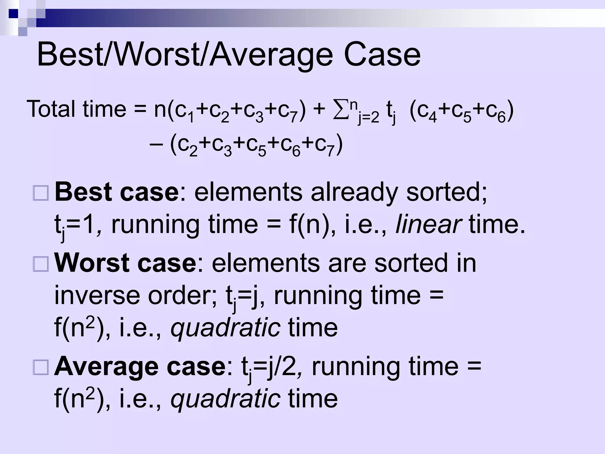
Total time = n(c1+c2+c3+c7) + nj=2 tj (c4+c5+c6)
– (c2+c3+c5+c6+c7)](https://image.slidesharecdn.com/lec1-101217091247-phpapp02/75/Lec1-14-2048.jpg)
![Example of Asymptotic Analysis
Algorithm prefixAverages1(X):
Input: An n-element array X of numbers.
Output: An n-element array A of numbers such that
A[i] is the average of elements X[0], ... , X[i].
for i 0 to n-1 do
a 0
for j 0 to i do n iterations
i iterations
a a + X[j] 1 with
A[i] a/(i+1) step i=0,1,2...n-
return array A 1
Analysis: running time is O(n2)](https://image.slidesharecdn.com/lec1-101217091247-phpapp02/75/Lec1-25-2048.jpg)
![A Better Algorithm
Algorithm prefixAverages2(X):
Input: An n-element array X of numbers.
Output: An n-element array A of numbers such
that A[i] is the average of elements X[0], ... , X[i].
s 0
for i 0 to n do
s s + X[i]
A[i] s/(i+1)
return array A
Analysis: Running time is O(n)](https://image.slidesharecdn.com/lec1-101217091247-phpapp02/75/Lec1-26-2048.jpg)


![Assertions
To prove correctness we associate a number of
assertions (statements about the state of the
execution) with specific checkpoints in the
algorithm.
E.g., A[1], …, A[k] form an increasing sequence
Preconditions – assertions that must be valid
before the execution of an algorithm or a
subroutine
Postconditions – assertions that must be valid
after the execution of an algorithm or a
subroutine](https://image.slidesharecdn.com/lec1-101217091247-phpapp02/75/Lec1-35-2048.jpg)
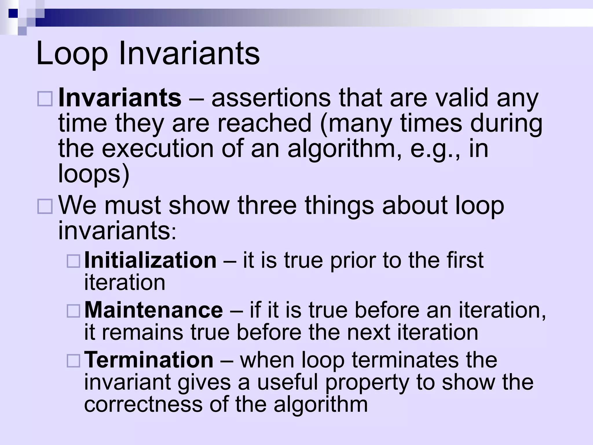
![Example of Loop Invariants (1)
Invariant: at the start of for j à 2 to length(A)
each for loop, A[1…j-1] do key à A[j]
i à j-1
consists of elements while i>0 and A[i]>key
originally in A[1…j-1] but do A[i+1] Ã A[i]
in sorted order i--
A[i+1] Ã key](https://image.slidesharecdn.com/lec1-101217091247-phpapp02/75/Lec1-37-2048.jpg)
![Example of Loop Invariants (2)
Invariant: at the start of for j à 2 to length(A)
each for loop, A[1…j-1] do key à A[j]
i à j-1
consists of elements while i>0 and A[i]>key
originally in A[1…j-1] but do A[i+1]Ã A[i]
in sorted order i--
A[i+1] Ã key
Initialization: j = 2, the invariant trivially holds
because A[1] is a sorted array ](https://image.slidesharecdn.com/lec1-101217091247-phpapp02/75/Lec1-38-2048.jpg)
![Example of Loop Invariants (3)
Invariant: at the start of for j à 2 to length(A)
each for loop, A[1…j-1] do key à A[j]
i à j-1
consists of elements while i>0 and A[i]>key
originally in A[1…j-1] but do A[i+1] Ã A[i]
in sorted order i--
A[i+1] Ã key
Maintenance: the inner while loop moves elements
A[j-1], A[j-2], …, A[j-k] one position right without
changing their order. Then the former A[j] element is
inserted into k-th position so that A[k-1] A[k]
A[k+1].
A[1…j-1] sorted + A[j] A[1…j] sorted](https://image.slidesharecdn.com/lec1-101217091247-phpapp02/75/Lec1-39-2048.jpg)
![Example of Loop Invariants (4)
Invariant: at the start of for j à 2 to length(A)
each for loop, A[1…j-1] do key à A[j]
i à j-1
consists of elements while i>0 and A[i]>key
originally in A[1…j-1] but do A[i+1] Ã A[i]
in sorted order i--
A[i+1] Ã key
Termination: the loop terminates, when j=n+1. Then
the invariant states: “A[1…n] consists of elements
originally in A[1…n] but in sorted order” ](https://image.slidesharecdn.com/lec1-101217091247-phpapp02/75/Lec1-40-2048.jpg)
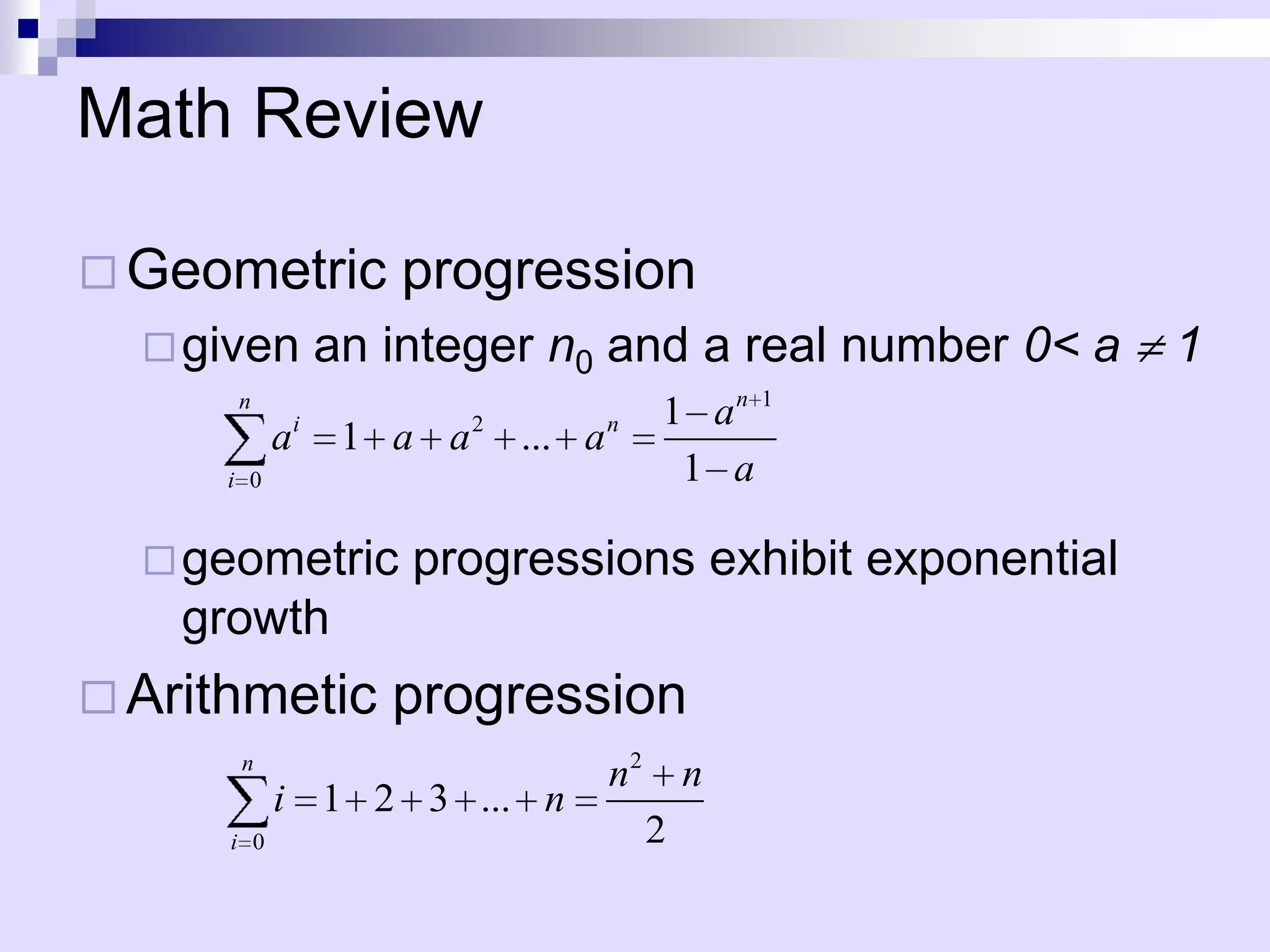
![Summations
Therunning time of insertion sort is
determined by a nested loop
for j 2 to length(A)
key A[j]
i j-1
while i>0 and A[i]>key
A[i+1] A[i]
i i-1
A[i+1] key
Nested loops correspond to summations
n
j 2
( j 1) O(n 2 )](https://image.slidesharecdn.com/lec1-101217091247-phpapp02/75/Lec1-43-2048.jpg)


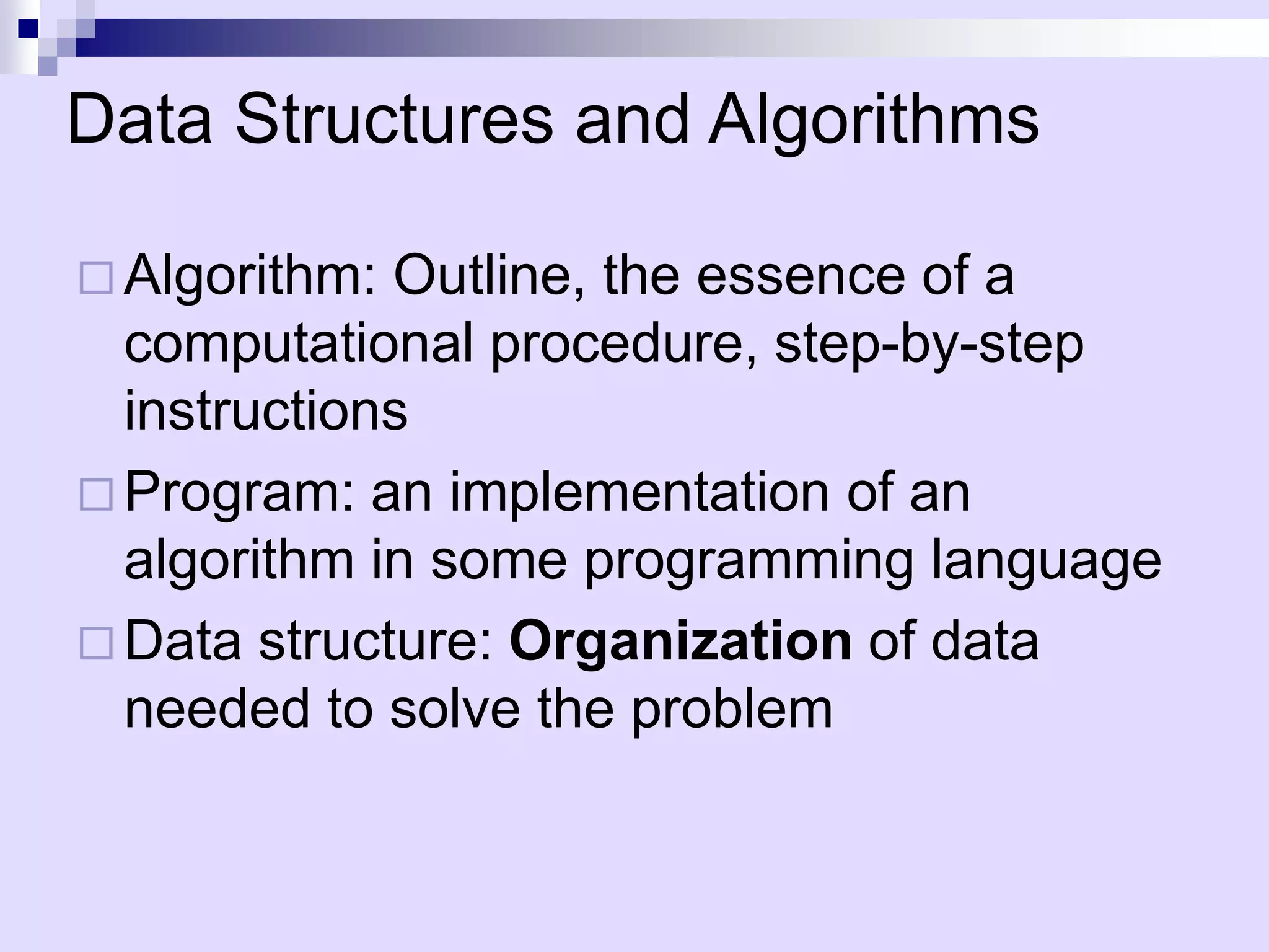
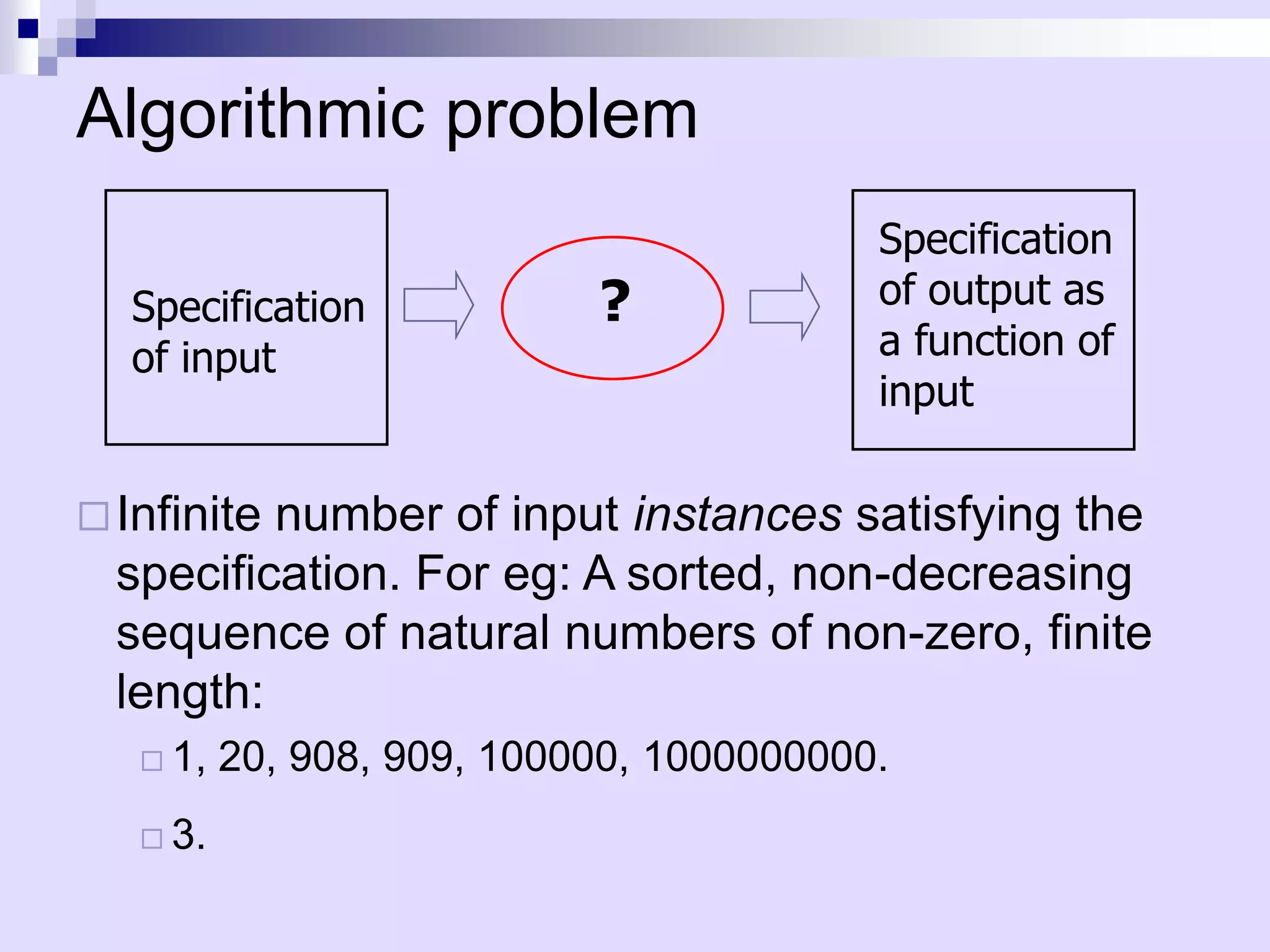
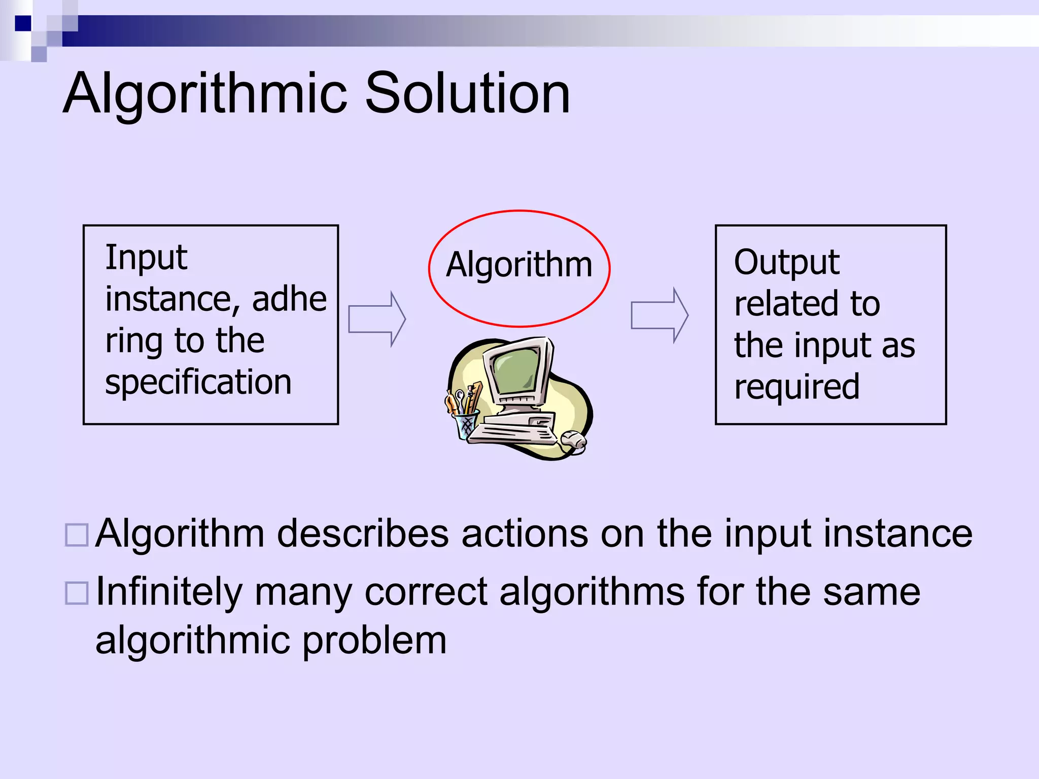
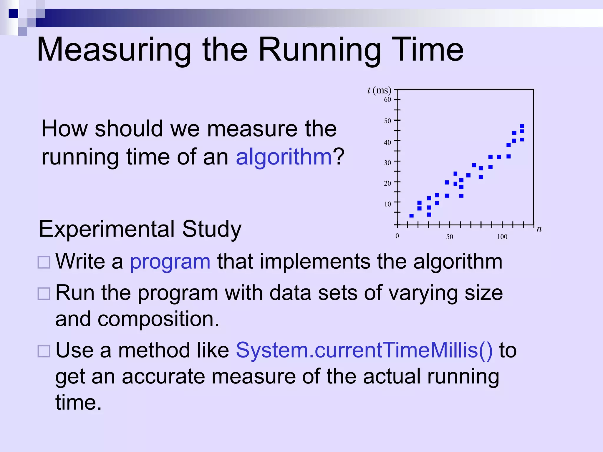
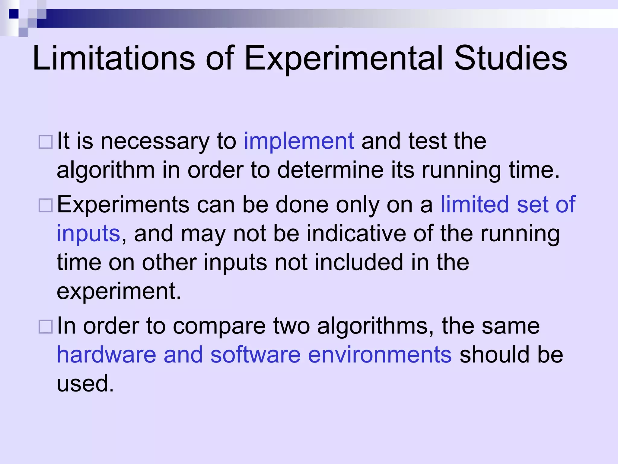
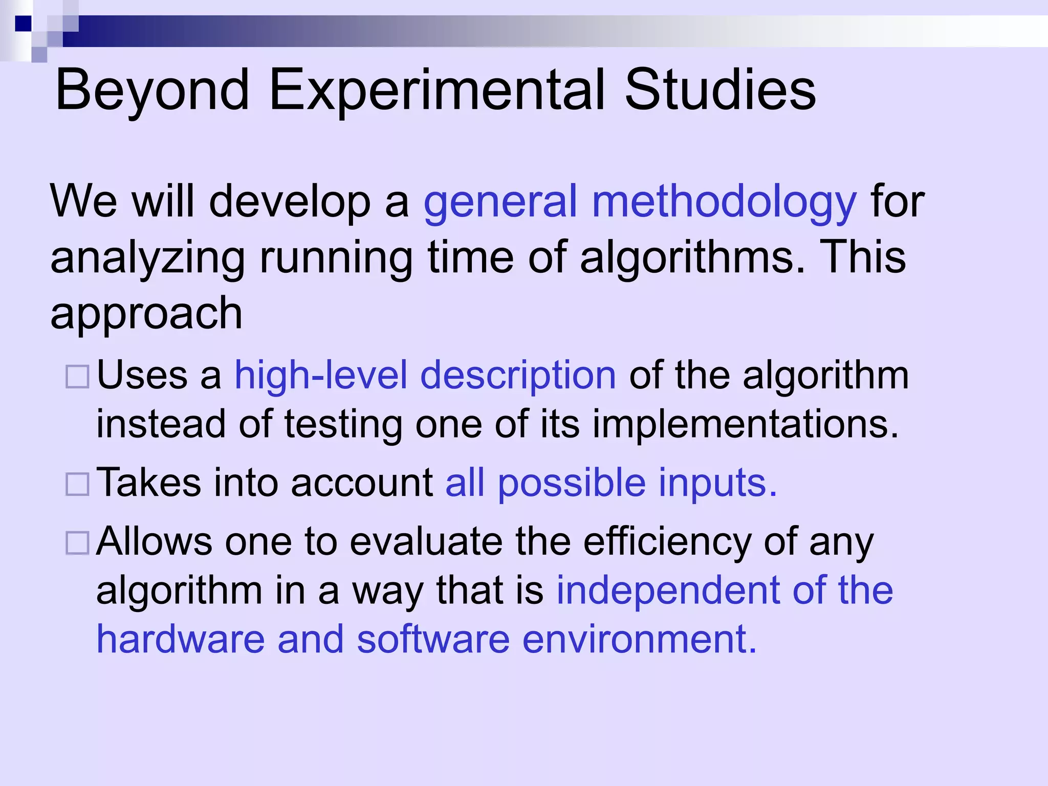
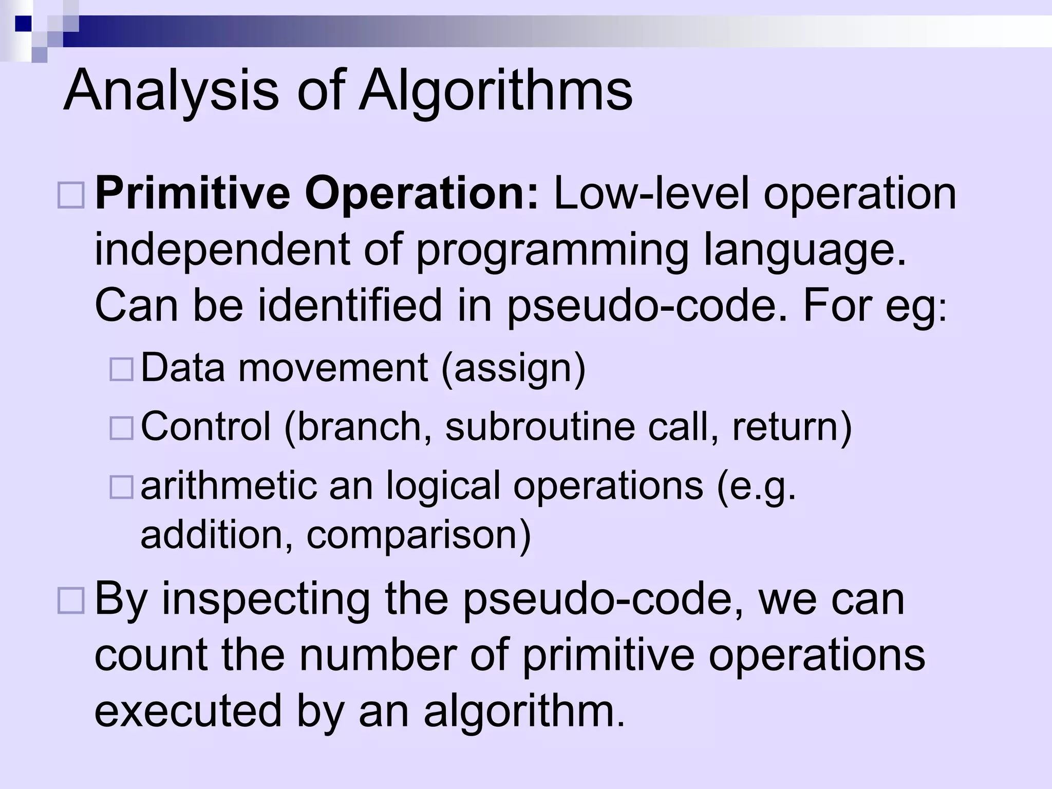
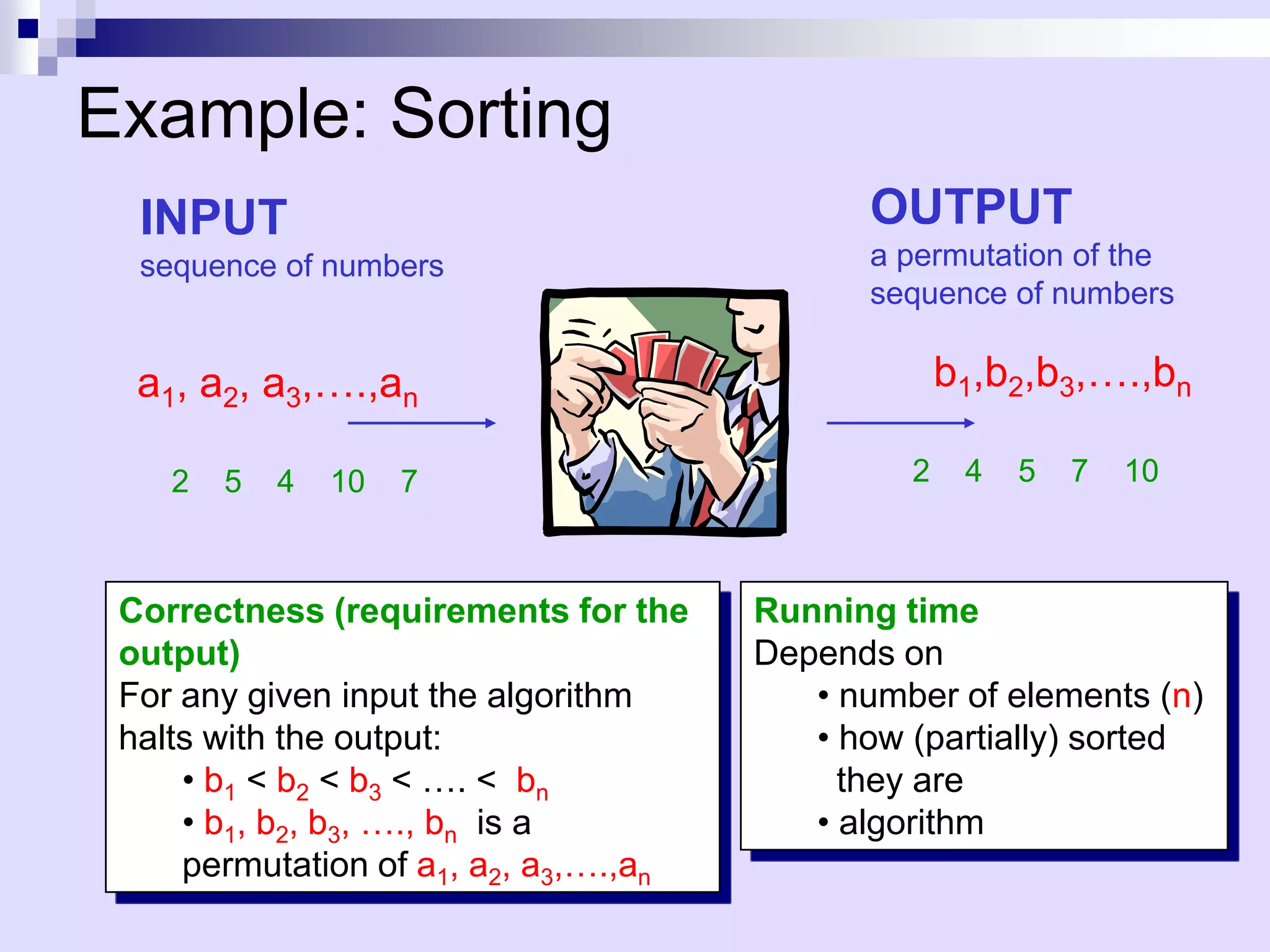
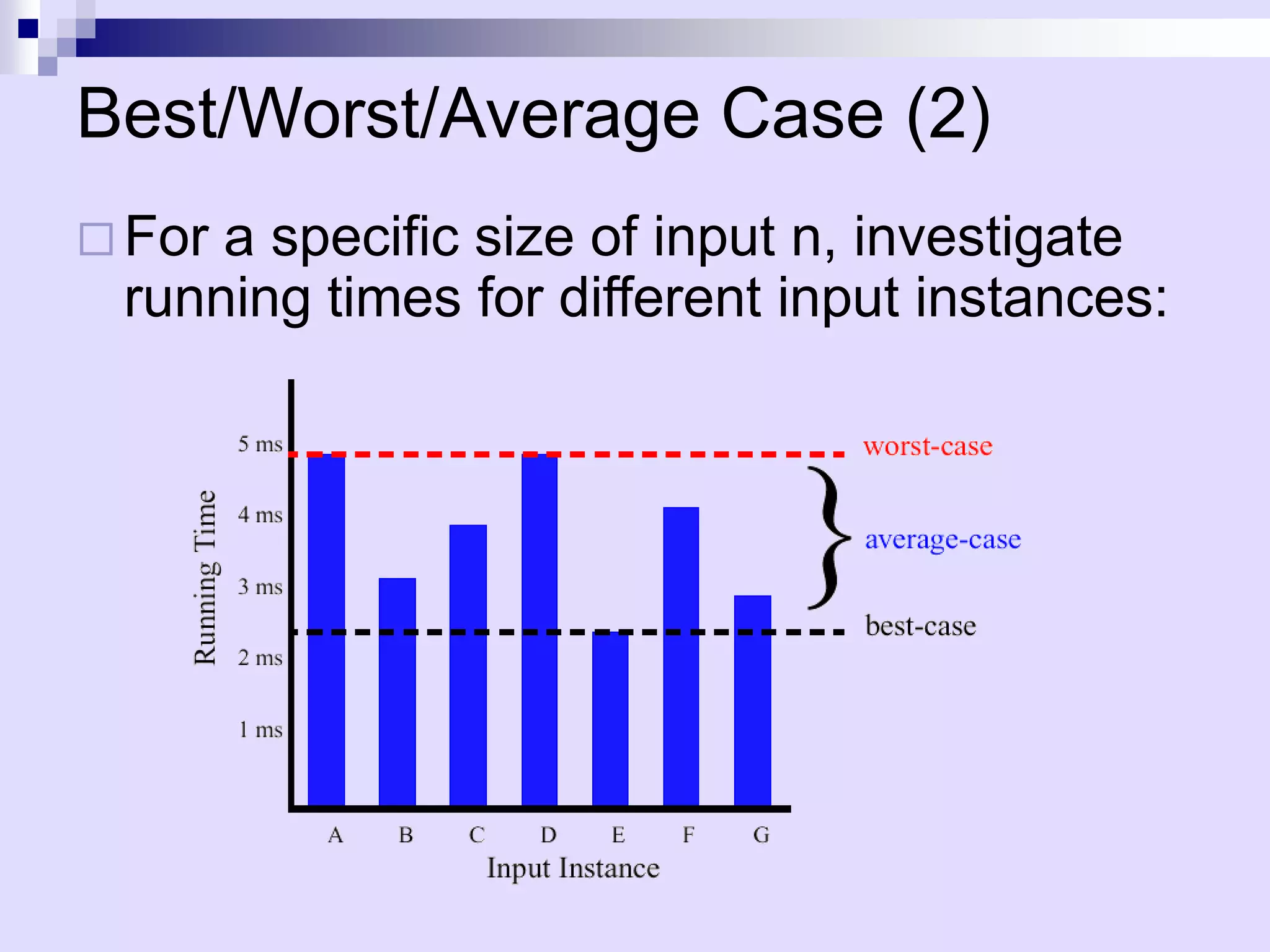
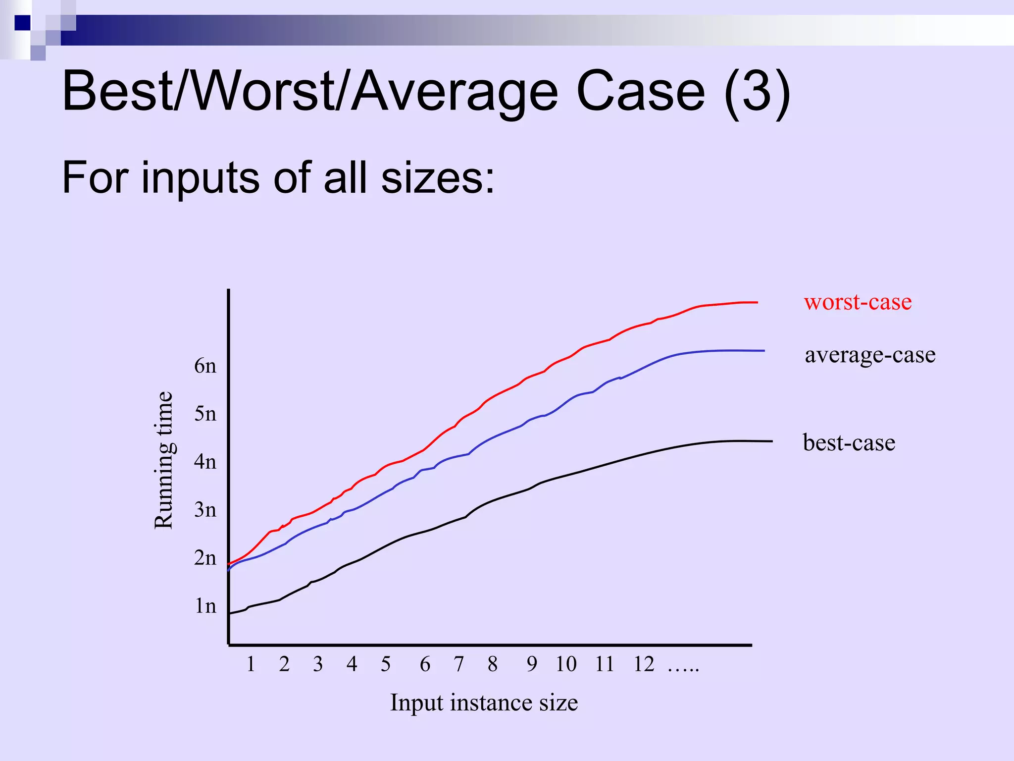
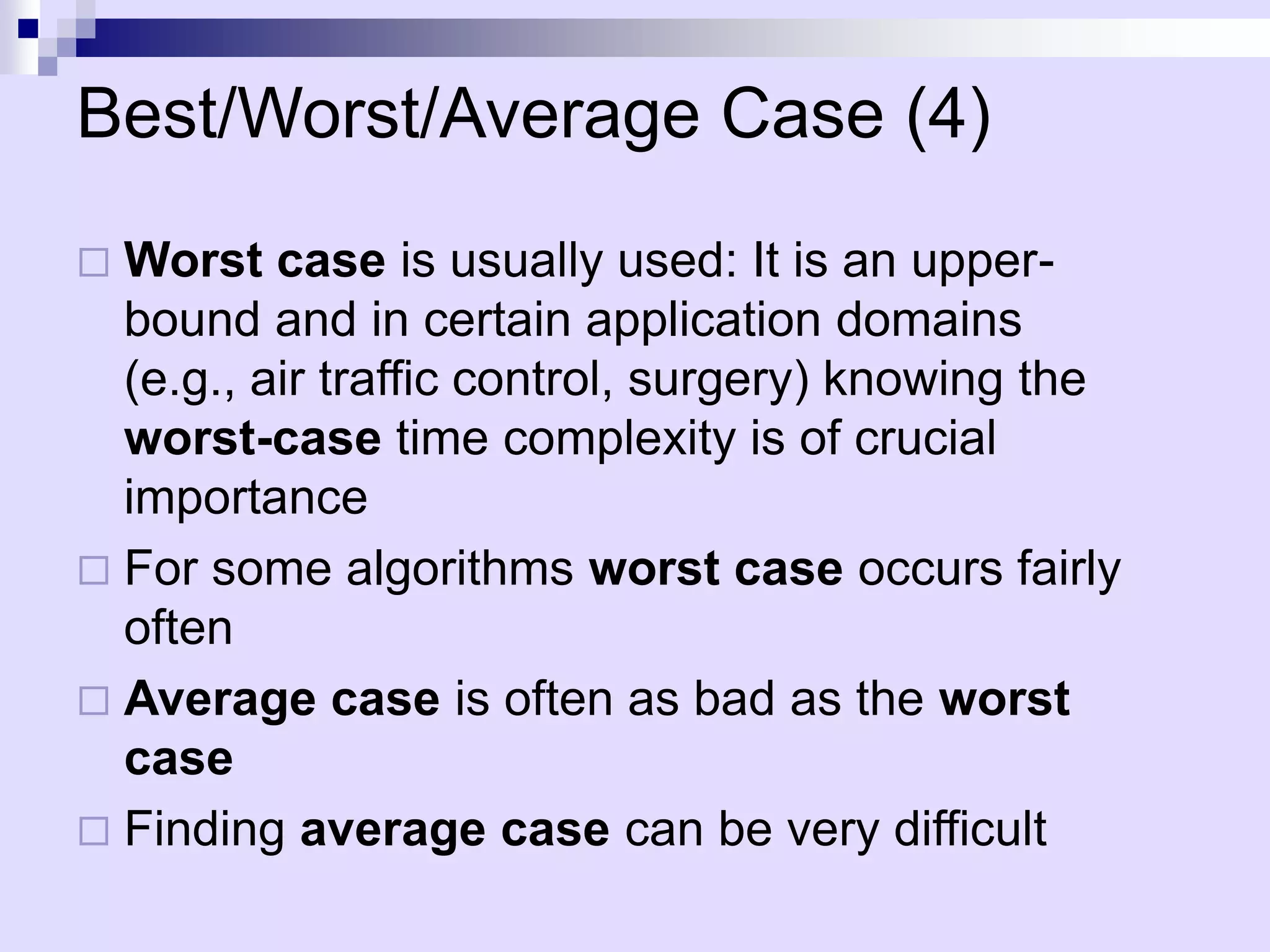
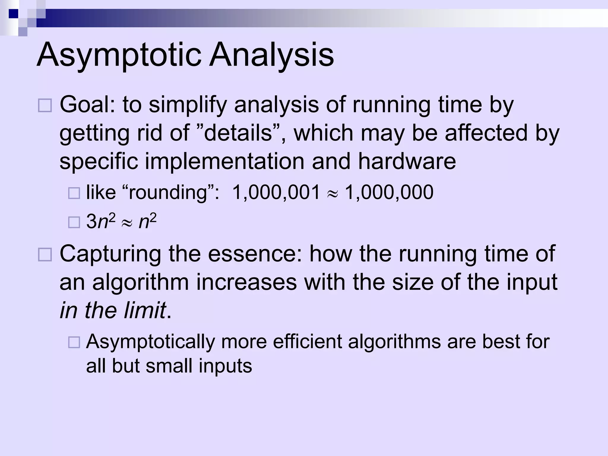
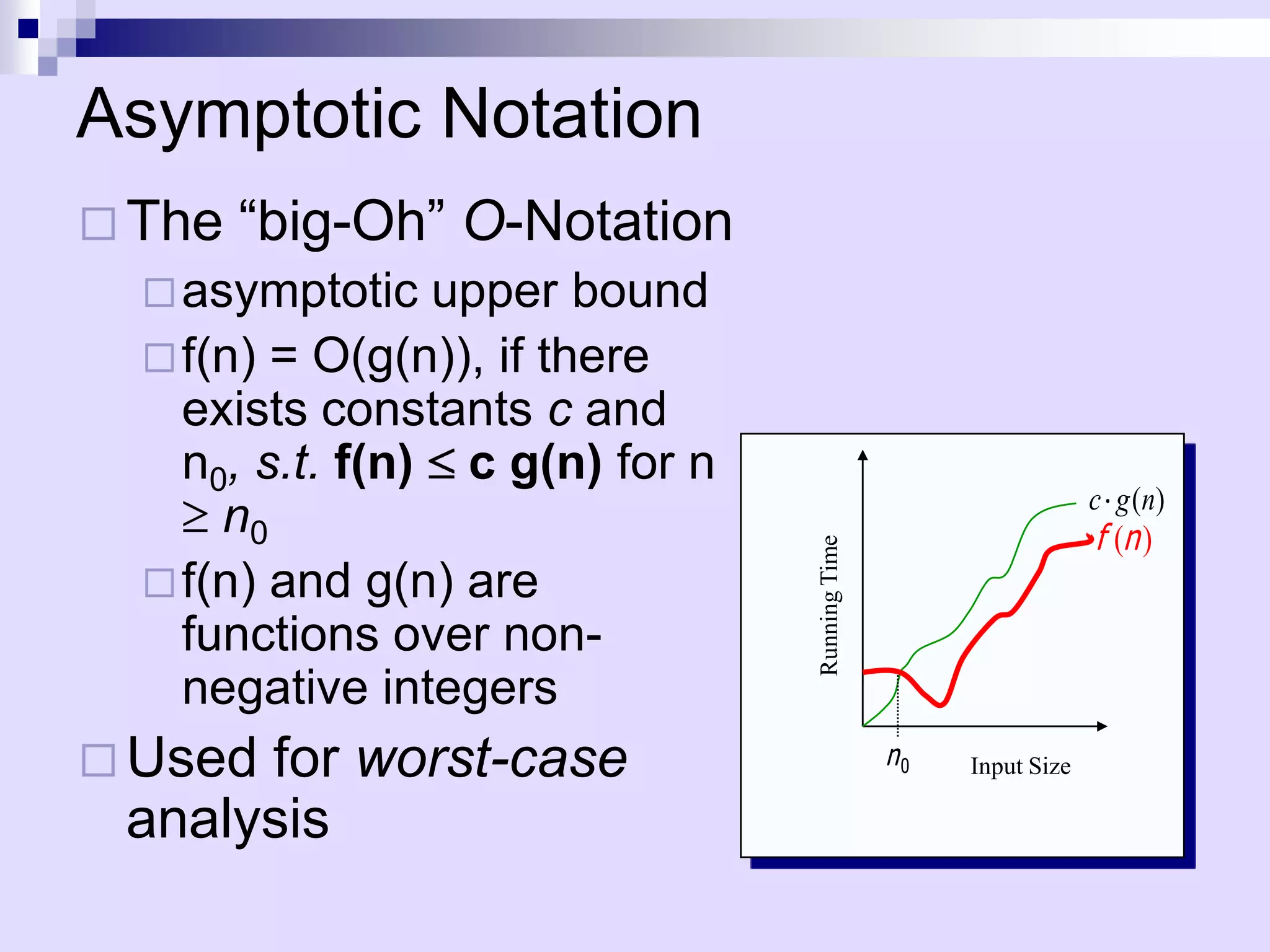
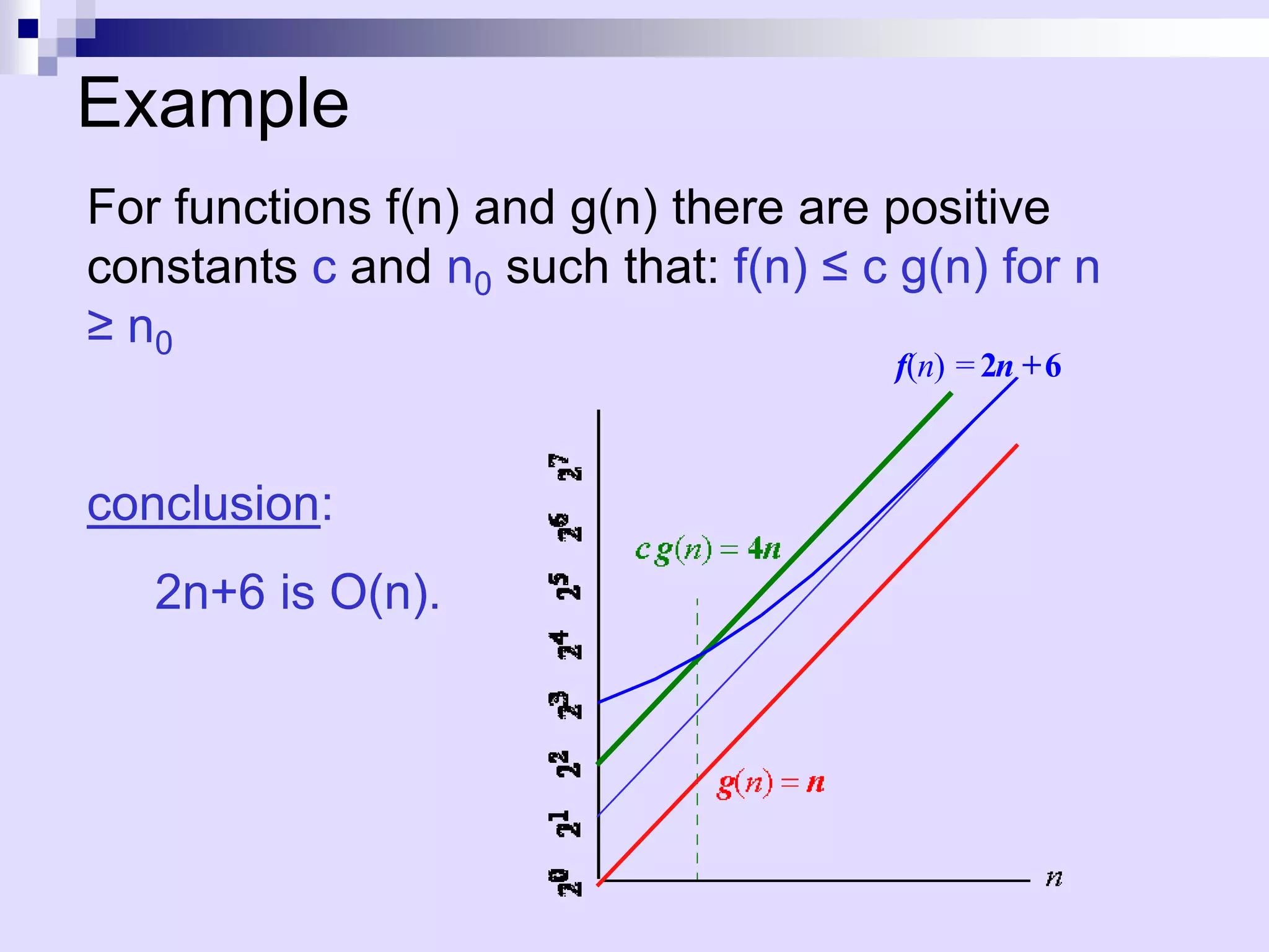
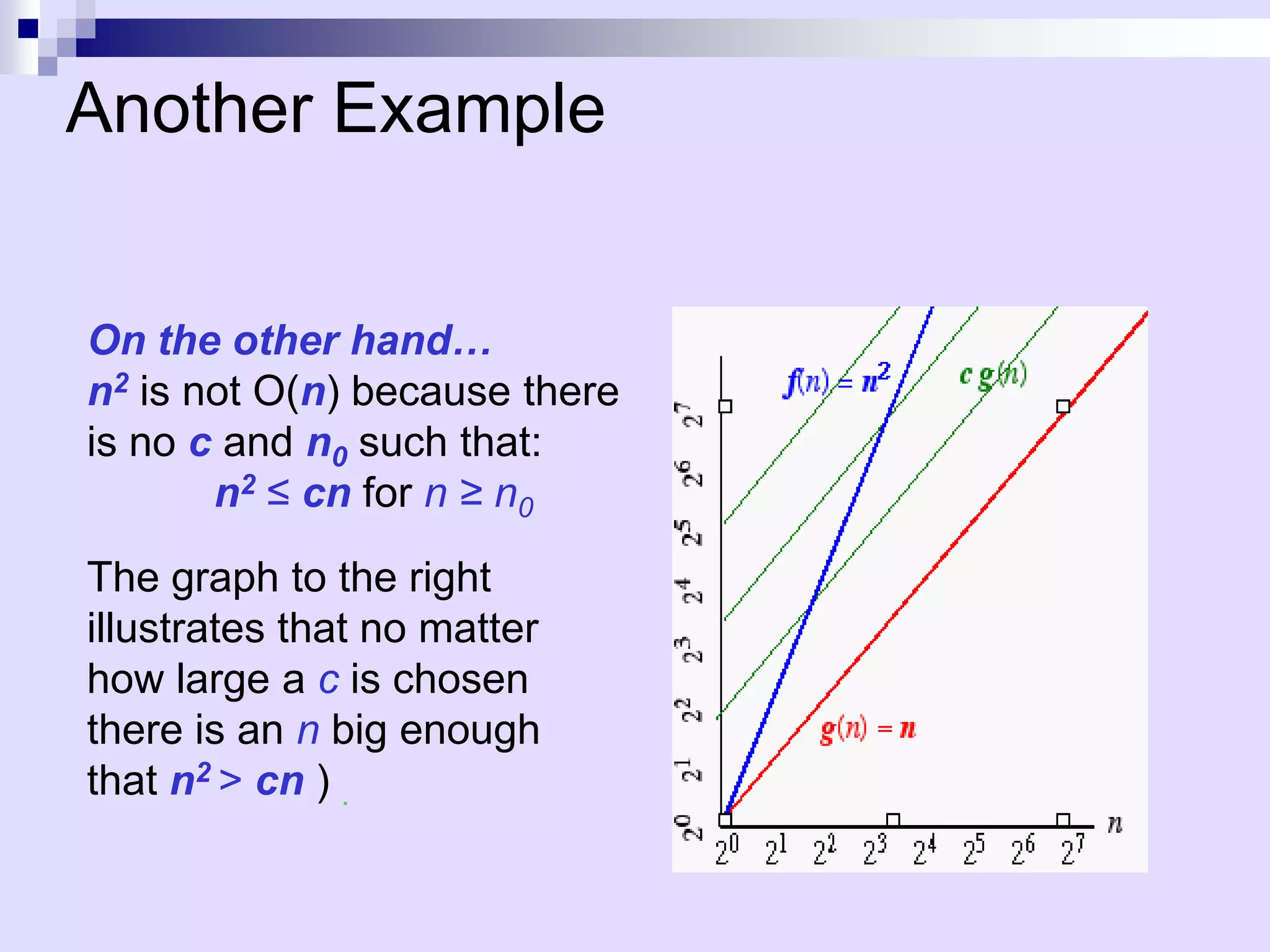
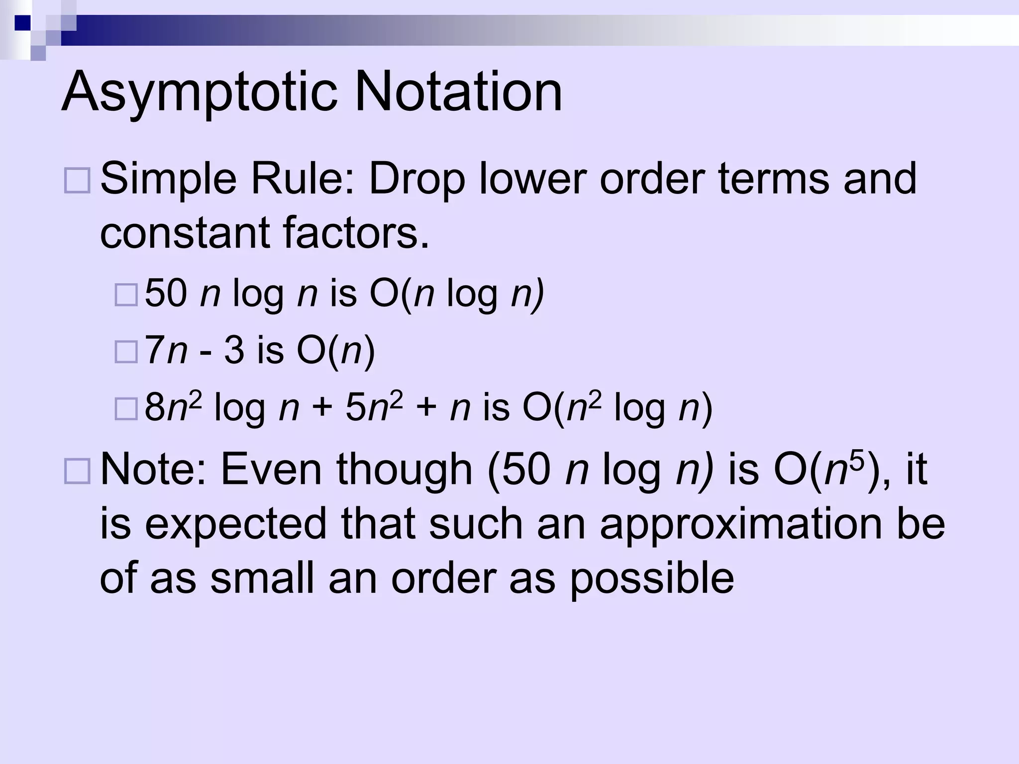
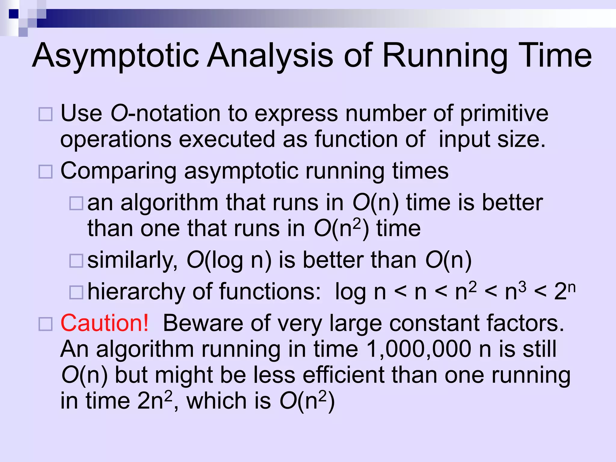
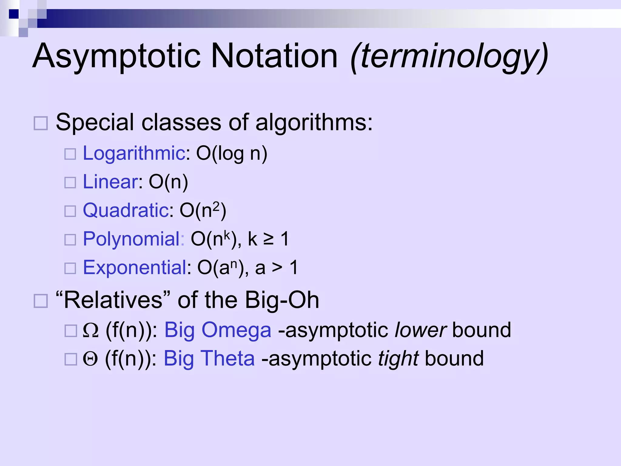
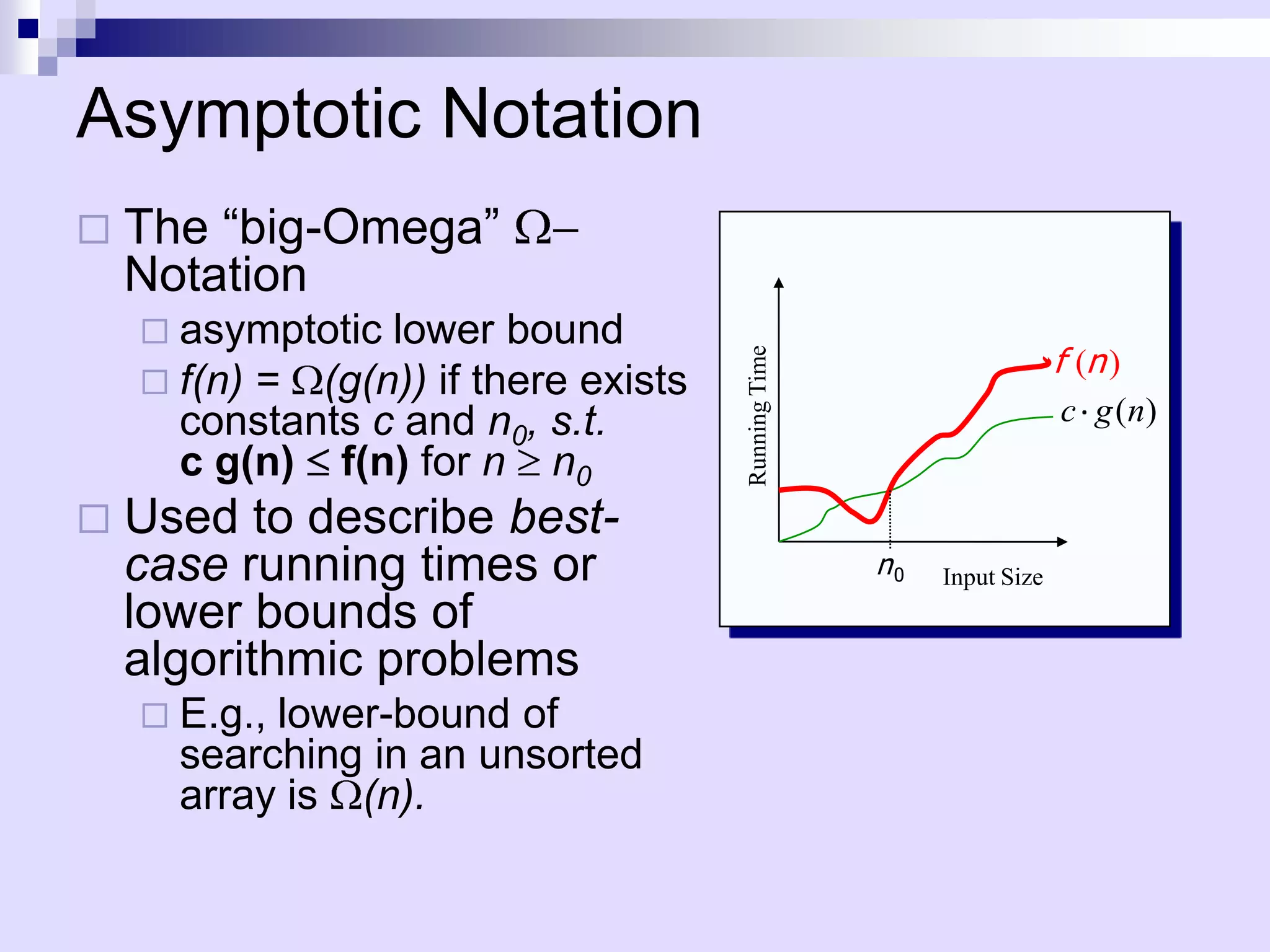
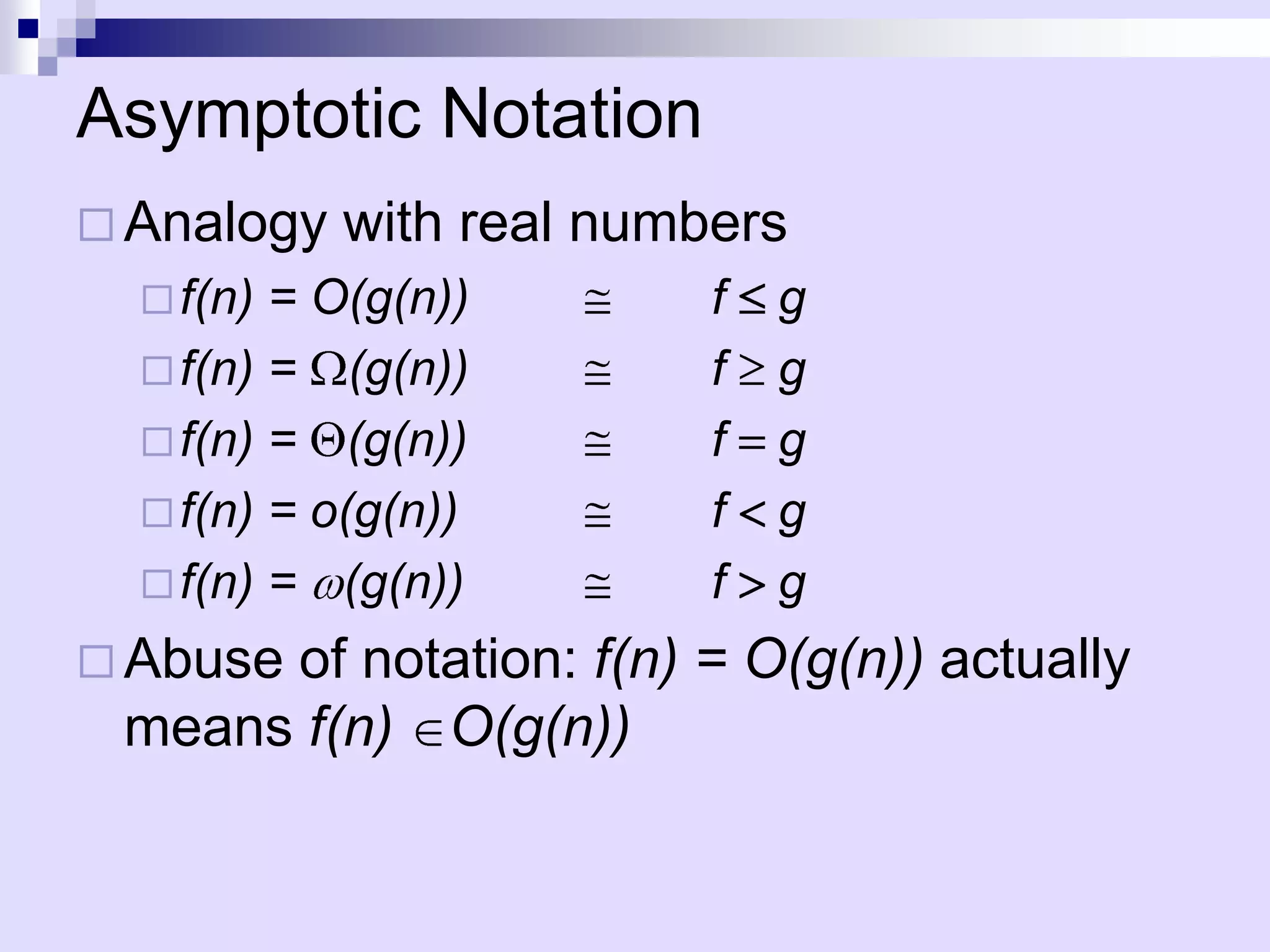
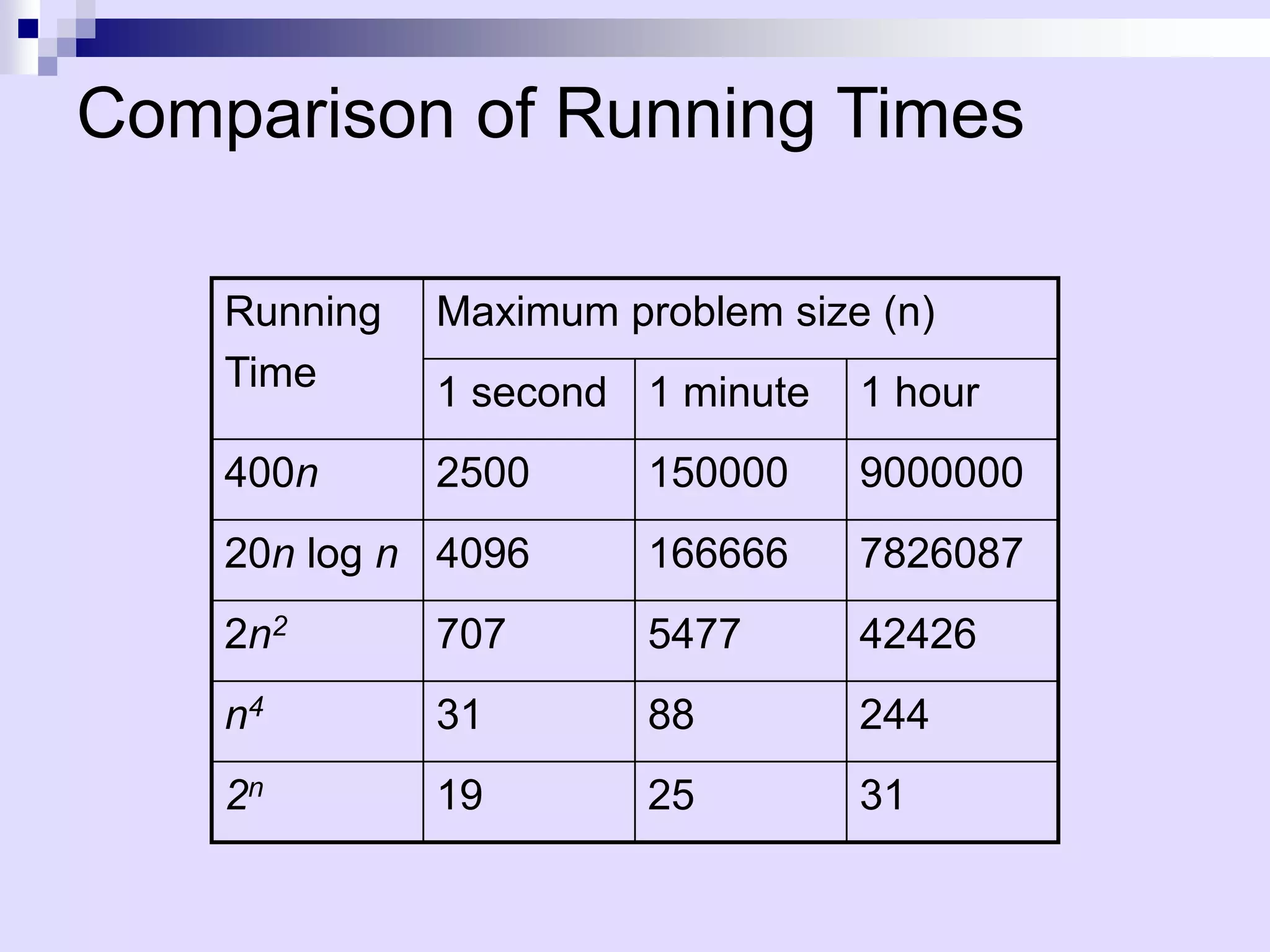
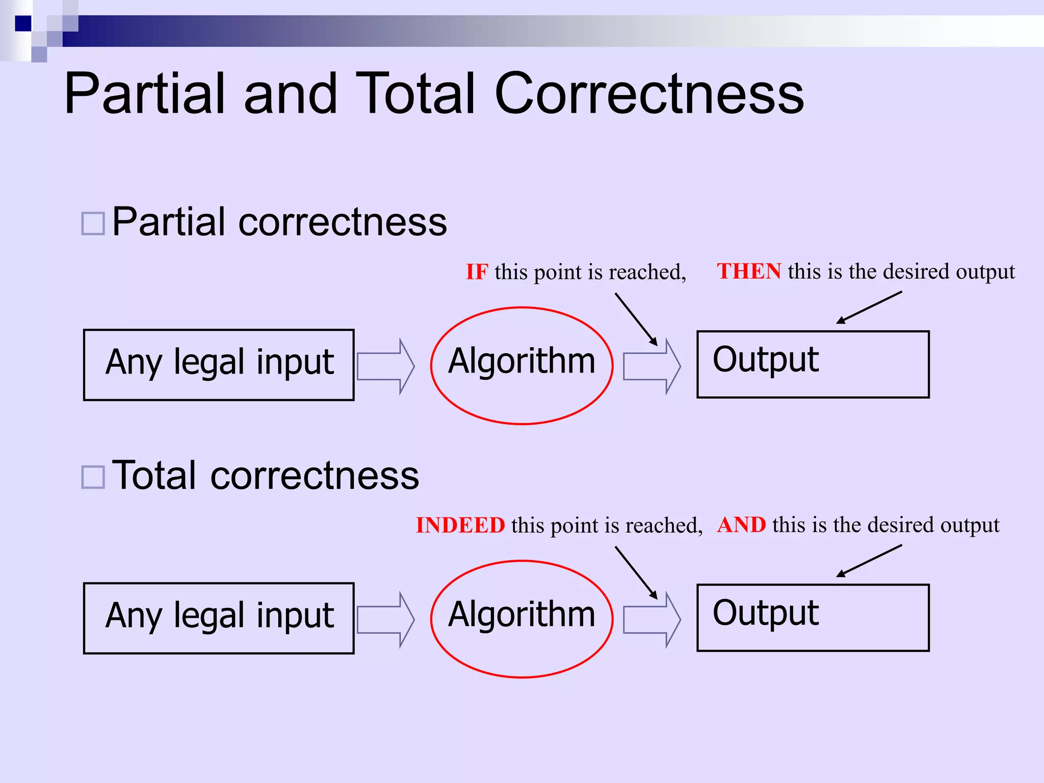
Data structures and algorithms involve organizing data to solve problems efficiently. An algorithm describes computational steps, while a program implements an algorithm. Key aspects of algorithms include efficiency as input size increases. Experimental studies measure running time but have limitations. Pseudocode describes algorithms at a high level. Analysis counts primitive operations to determine asymptotic running time, ignoring constant factors. The best, worst, and average cases analyze efficiency. Asymptotic notation like Big-O simplifies analysis by focusing on how time increases with input size.