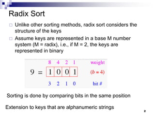
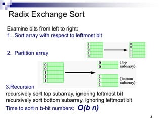
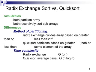
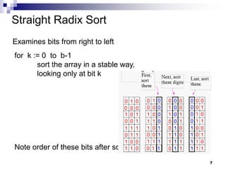
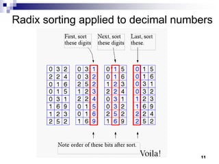
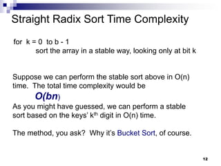
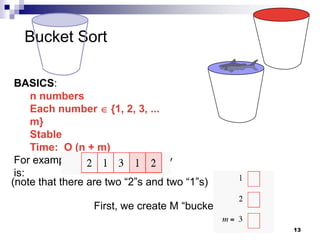
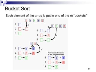
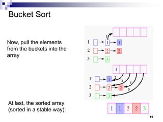
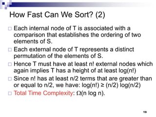
Radix sort considers the structure of keys and sorts based on comparing bits in the same position. Bucket sort is used to stably sort based on individual bits, with time complexity O(bn) for b-bit keys. While comparison-based sorting requires Ω(n log n) time, radix sort circumvents this lower bound by exploiting key structure rather than just comparisons.

1. More Sorting
 radix sort
 bucket sort
 in-place sorting
 how fast can we sort?
1

2. Radix Sort
 Unlike other sorting methods, radix sort considers the
structure of the keys
 Assume keys are represented in a base M number
system (M = radix), i.e., if M = 2, the keys are
represented in binary
Sorting is done by comparing bits in the same position
Extension to keys that are alphanumeric strings
2

3. Radix Exchange Sort
Examine bits from left to right:
1. Sort array with respect to leftmost bit
2. Partition array
3.Recursion
recursively sort top subarray, ignoring leftmost bit
recursively sort bottom subarray, ignoring leftmost bit
Time to sort n b-bit numbers: O(b n)
3

4. Radix Exchange Sort
How do we do the sort from the previous page? Same idea as
partition in Quicksort.
repeat
scan top-down to find key starting with 1;
scan bottom-up to find key starting with 0
exchange keys;
until scan indices cross;
4

5. Radix Exchange Sort
5

6. Radix Exchange Sort vs. Quicksort
Similarities
both partition array
both recursively sort sub-arrays
Differences
Method of partitioning
radix exchange divides array based on greater
than or less than 2b-1
quicksort partitions based on greater than or
less than some element of the array
Time complexity
Radix exchange O (bn)
Quicksort average case O (n log n)
6

7. Straight Radix Sort
Examines bits from right to left
for k := 0 to b-1
sort the array in a stable way,
looking only at bit k
Note order of these bits after sort.
7

8. What is “sort in a stable way”!!!
In a stable sort, the initial relative order of equal keys is
unchanged. For example, observe the first step of the sort
from the previous page:
Note that the relative order of those keys ending with 0
is unchanged, and the same is true for elements
ending in 1
8

9. The Algorithm is Correct (right?)
We show that any two keys are in the correct relative order
at the end of the algorithm
Given two keys, let k be the leftmost bit-position where
they differ
At step k the two keys are put in the correct relative
order
Because of stability, the successive steps do not
change the relative order of the two keys
9

10. For Instance,
Consider a sort on an array with these two keys:
10

11. Radix sorting applied to decimal numbers
11

12. Straight Radix Sort Time Complexity
for k = 0 to b - 1
sort the array in a stable way, looking only at bit k
Suppose we can perform the stable sort above in O(n)
time. The total time complexity would be
O(bn)
As you might have guessed, we can perform a stable
sort based on the keys’ kth digit in O(n) time.
The method, you ask? Why it’s Bucket Sort, of course.
12

13. Bucket Sort
BASICS:
n numbers
Each number  {1, 2, 3, ...
m}
Stable
Time: O (n + m)
For example, m = 3 and our array
is:
(note that there are two “2”s and two “1”s)
First, we create M “buckets”
13

14. Bucket Sort
Each element of the array is put in one of the m “buckets”
14

15. Bucket Sort
Now, pull the elements
from the buckets into the
array
At last, the sorted array
(sorted in a stable way):
15

16. In-Place Sorting
 A sorting algorithm is said to be in-place if
 it uses no auxiliary data structures (however, O(1)
auxiliary variables are allowed)
 it updates the input sequence only by means of
operations replaceElement and swapElements
 Which sorting algorithms seen can be made to
work in place?
16

17. Lower Bd. for Comparison Based Sorting
 internal node: comparison
 external node: permutation
 algorithm execution: root-to-leaf path
17

18. How Fast Can We Sort?
 How Fast Can We Sort?
 Proposition: The running time of any
comparison-based algorithm for sorting an n-
element sequence S is (n log n).
 Justification: The running time of a
comparison-based sorting algorithm must be
equal to or greater than the depth of the
decision tree T associated with this algorithm.
18

19. How Fast Can We Sort? (2)
 Each internal node of T is associated with a
comparison that establishes the ordering of two
elements of S.
 Each external node of T represents a distinct
permutation of the elements of S.
 Hence T must have at least n! external nodes which
again implies T has a height of at least log(n!)
 Since n! has at least n/2 terms that are greater than
or equal to n/2, we have: log(n!) ≥ (n/2) log(n/2)
 Total Time Complexity: (n log n).
19