Recurrences

Algorithms

Sandeep Kumar Poonia
Head Of Dept. CS/IT
B.E., M.Tech., UGC-NET
LM-IAENG, LM-IACSIT,LM-CSTA, LM-AIRCC, LM-SCIEI, AM-UACEE

Algorithms
Merge Sort
Solving Recurrences
The Master Theorem
Introduction to heapsort
Quicksort


Merge Sort
MergeSort(A, left, right) {
if (left < right) {
mid = floor((left + right) / 2);
MergeSort(A, left, mid);
MergeSort(A, mid+1, right);
Merge(A, left, mid, right);
}
}
// Merge() takes two sorted subarrays of A and
// merges them into a single sorted subarray of A
//
(how long should this take?)


Merge Sort: Example


Show MergeSort() running on the array
A = {10, 5, 7, 6, 1, 4, 8, 3, 2, 9};


Analysis of Merge Sort
Statement

Effort

MergeSort(A, left, right) {
if (left < right) {
mid = floor((left + right) / 2);
MergeSort(A, left, mid);
MergeSort(A, mid+1, right);
Merge(A, left, mid, right);
}
}
 So T(n) = (1) when n = 1, and

2T(n/2) + (n) when n > 1


So what (more succinctly) is T(n)?


T(n)
(1)
(1)
T(n/2)
T(n/2)
(n)

Recurrences


The expression:
c
n 1



T ( n)  
n
2T    cn n  1
 2


is a recurrence.


Recurrence: an equation that describes a function
in terms of its value on smaller functions


Recurrence Examples
0
n0

s ( n)  
c  s(n  1) n  0

0
n0

s ( n)  
n  s(n  1) n  0

c
n 1



T ( n)  
n
2T    c n  1
 2




c
n 1

T ( n)  
 n
aT    cn n  1
 b


Solving Recurrences
Substitution method
 Iteration method
 Master method



Solving Recurrences


The substitution method





A.k.a. the “making a good guess method”
Guess the form of the answer, then use induction
to find the constants and show that solution works
Examples:
= 2T(n/2) + (n)  T(n) = (n lg n)
 T(n) = 2T(n/2) + n  ???
 T(n)


Solving Recurrences







Examples:
= 2T(n/2) + (n)  T(n) = (n lg n)
 T(n) = 2T(n/2) + n  T(n) = (n lg n)
 T(n) = 2T(n/2 )+ 17) + n  ???
 T(n)


Solving Recurrences







Examples:
= 2T(n/2) + (n)  T(n) = (n lg n)
 T(n) = 2T(n/2) + n  T(n) = (n lg n)
 T(n) = 2T(n/2+ 17) + n  (n lg n)
 T(n)


Solving Recurrences


Another option is the “iteration method”






Expand the recurrence
Work some algebra to express as a summation
Evaluate the summation

We will show several examples


0
n0

s ( n)  
c  s(n  1) n  0


s(n) =
c + s(n-1)
c + c + s(n-2)
2c + s(n-2)
2c + c + s(n-3)
3c + s(n-3)
…
kc + s(n-k) = ck + s(n-k)


0
n0

s ( n)  
c  s(n  1) n  0


So far for n >= k we have




s(n) = ck + s(n-k)

What if k = n?


s(n) = cn + s(0) = cn


0
n0

s ( n)  
c  s(n  1) n  0






s(n) = ck + s(n-k)

What if k = n?


s(n) = cn + s(0) = cn

0
n0

s ( n)  
c  s(n  1) n  0



So



Thus in general


s(n) = cn


0
n0

s ( n)  
n  s(n  1) n  0


=
=
=
=
=
=

s(n)
n + s(n-1)
n + n-1 + s(n-2)
n + n-1 + n-2 + s(n-3)
n + n-1 + n-2 + n-3 + s(n-4)
…
n + n-1 + n-2 + n-3 + … + n-(k-1) + s(n-k)


0
n0

s ( n)  
n  s(n  1) n  0


=
=
=
=
=
=

s(n)
n + s(n-1)
n + n-1 + s(n-2)
n + n-1 + n-2 + s(n-3)
n + n-1 + n-2 + n-3 + s(n-4)
…
n + n-1 + n-2 + n-3 + … + n-(k-1) + s(n-k)
n

=

i

i  n  k 1


 s(n  k )

0
n0

s ( n)  
n  s(n  1) n  0


n

i

i  n  k 1


 s(n  k )

0
n0

s ( n)  
n  s(n  1) n  0


n

i

 s(n  k )

i  n  k 1



What if k = n?


0
n0

s ( n)  
n  s(n  1) n  0


n

i

 s(n  k )

i  n  k 1



What if k = n?

n 1
 i  s(0)   i  0  n 2
i 1
i 1
n


n

0
n0

s ( n)  
n  s(n  1) n  0


n

i

 s(n  k )

i  n  k 1



What if k = n?

n 1
 i  s(0)   i  0  n 2
i 1
i 1
n



Thus in general

n 1
s ( n)  n
2


n

c
n 1

 n
T (n)  2T
   c n 1
 2



T(n) =
2T(n/2) + c
2(2T(n/2/2) + c) + c
22T(n/22) + 2c + c
22(2T(n/22/2) + c) + 3c
23T(n/23) + 4c + 3c
23T(n/23) + 7c
23(2T(n/23/2) + c) + 7c
24T(n/24) + 15c
…
2kT(n/2k) + (2k - 1)c


c
n 1

 n
T (n)  2T
   c n 1
 2



So far for n > 2k we have




T(n) = 2kT(n/2k) + (2k - 1)c

What if k = lg n?


T(n) = 2lg n T(n/2lg n) + (2lg n - 1)c
= n T(n/n) + (n - 1)c
= n T(1) + (n-1)c
= nc + (n-1)c = (2n - 1)c


The Master Theorem


Given: a divide and conquer algorithm






An algorithm that divides the problem of size n
into a subproblems, each of size n/b
Let the cost of each stage (i.e., the work to divide
the problem + combine solved subproblems) be
described by the function f(n)

Then, the Master Theorem gives us a
cookbook for the algorithm’s running time:


The Master Theorem


if T(n) = aT(n/b) + f(n) then



 n logb a




logb a
T (n)   n
log n


 f (n) 












f (n)  O n logb a 


  0
logb a
f ( n)   n

 c 1


f (n)   n logb a  AND

af (n / b)  cf (n) for large n















Using The Master Method


T(n) = 9T(n/3) + n




a=9, b=3, f(n) = n
nlog a = nlog 9 = (n2)
Since f(n) = O(nlog 9 - ), where =1, case 1 applies:
b

3

3







T (n)   nlogb a when f (n)  O nlogb a 


Thus the solution is T(n) = (n2)




Sorting Revisited


So far we’ve talked about two algorithms to
sort an array of numbers





What is the advantage of merge sort?
What is the advantage of insertion sort?

Next on the agenda: Heapsort


Combines advantages of both previous algorithms


Heaps


A heap can be seen as a complete binary tree:
16

14

10

8

2




7

4

9

1

What makes a binary tree complete?
Is the example above complete?


3

Heaps


A heap can be seen as a complete binary tree:
16

14

10

8

2



7

4

1

9

1

1

3

1

1

The book calls them “nearly complete” binary
trees; can think of unfilled slots as null pointers


1

Heaps


In practice, heaps are usually implemented as
arrays:
16
14

A = 16 14 10 8

7

9

3

2

4

8

1 =
2


10
7

4

1

9

3

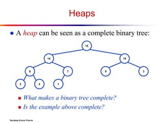
Heaps


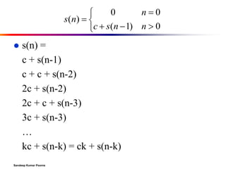
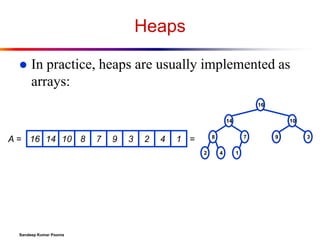
To represent a complete binary tree as an array:







The root node is A[1]
Node i is A[i]
The parent of node i is A[i/2] (note: integer divide)
The left child of node i is A[2i]
The right child of node i is A[2i + 1]
16
14

A = 16 14 10 8

7

9

3

2

4

8

1 =
2


10
7

4

1

9

3

Referencing Heap Elements


So…
Parent(i) { return i/2; }
Left(i) { return 2*i; }
right(i) { return 2*i + 1; }

An aside: How would you implement this
most efficiently?
 Another aside: Really?



The Heap Property


Heaps also satisfy the heap property:
A[Parent(i)]  A[i]
for all nodes i > 1






In other words, the value of a node is at most the
value of its parent
Where is the largest element in a heap stored?

Definitions:




The height of a node in the tree = the number of
edges on the longest downward path to a leaf
The height of a tree = the height of its root


Heap Height
What is the height of an n-element heap? Why?
 This is nice: basic heap operations take at most
time proportional to the height of the heap



Heap Operations: Heapify()


Heapify(): maintain the heap property







Given: a node i in the heap with children l and r
Given: two subtrees rooted at l and r, assumed to
be heaps
Problem: The subtree rooted at i may violate the
heap property (How?)
Action: let the value of the parent node “float
down” so subtree at i satisfies the heap property
 What

do you suppose will be the basic operation
between i, l, and r?


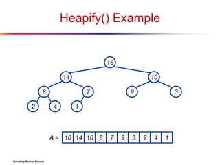
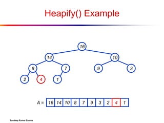
Heap Operations: Heapify()
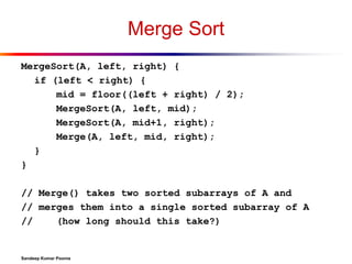
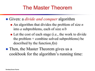
Heapify(A, i)
{
l = Left(i); r = Right(i);
if (l <= heap_size(A) && A[l] > A[i])
largest = l;
else
largest = i;
if (r <= heap_size(A) && A[r] > A[largest])
largest = r;
if (largest != i)
Swap(A, i, largest);
Heapify(A, largest);
}

Heapify() Example

16
4

10

14
2

7
8

3

1

A = 16 4 10 14 7


9

9

3

2

8

1

Heapify() Example

16
14

10

4
2

7
8

3

1

A = 16 14 10 4


9

7

9

3

2

8

1

Heapify() Example

16
14

10

8
2

7
4

3

1

A = 16 14 10 8


9

7

9

3

2

4

1

Analyzing Heapify(): Informal
Aside from the recursive call, what is the
running time of Heapify()?
 How many times can Heapify() recursively
call itself?
 What is the worst-case running time of
Heapify() on a heap of size n?



Analyzing Heapify(): Formal
Fixing up relationships between i, l, and r
takes (1) time
 If the heap at i has n elements, how many
elements can the subtrees at l or r have?




Draw it

Answer: 2n/3 (worst case: bottom row 1/2 full)
 So time taken by Heapify() is given by


T(n)  T(2n/3) + (1)

Analyzing Heapify(): Formal
So we have
T(n)  T(2n/3) + (1)
 By case 2 of the Master Theorem,
T(n) = O(lg n)
 Thus, Heapify() takes linear time



Heap Operations: BuildHeap()


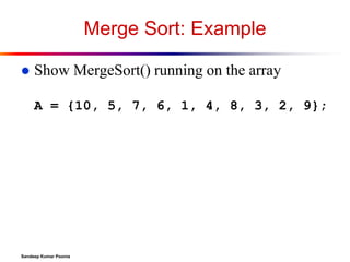
We can build a heap in a bottom-up manner by
running Heapify() on successive subarrays




Fact: for array of length n, all elements in range
A[n/2 + 1 .. n] are heaps (Why?)
So:
 Walk

backwards through the array from n/2 to 1, calling
Heapify() on each node.

 Order

of processing guarantees that the children of node
i are heaps when i is processed


BuildHeap()
// given an unsorted array A, make A a heap
BuildHeap(A)
{
heap_size(A) = length(A);
for (i = length[A]/2 downto 1)
Heapify(A, i);
}


BuildHeap() Example


Work through example
A = {4, 1, 3, 2, 16, 9, 10, 14, 8, 7}
4
1

3

2
14


16
8

7

9

10

Analyzing BuildHeap()


Each call to Heapify() takes O(lg n) time

There are O(n) such calls (specifically, n/2)
 Thus the running time is O(n lg n)







Is this a correct asymptotic upper bound?
Is this an asymptotically tight bound?

A tighter bound is O(n)


How can this be? Is there a flaw in the above
reasoning?


Analyzing BuildHeap(): Tight


To Heapify() a subtree takes O(h) time
where h is the height of the subtree



h = O(lg m), m = # nodes in subtree
The height of most subtrees is small

Fact: an n-element heap has at most n/2h+1
nodes of height h
 CLR 7.3 uses this fact to prove that
BuildHeap() takes O(n) time



Heapsort


Given BuildHeap(), an in-place sorting
algorithm is easily constructed:



Maximum element is at A[1]
Discard by swapping with element at A[n]
 Decrement

heap_size[A]
 A[n] now contains correct value


Restore heap property at A[1] by calling
Heapify()



Repeat, always swapping A[1] for A[heap_size(A)]


Heapsort
Heapsort(A)
{
BuildHeap(A);
for (i = length(A) downto 2)
{
Swap(A[1], A[i]);
heap_size(A) -= 1;
Heapify(A, 1);
}
}


Analyzing Heapsort
The call to BuildHeap() takes O(n) time
 Each of the n - 1 calls to Heapify() takes
O(lg n) time
 Thus the total time taken by HeapSort()
= O(n) + (n - 1) O(lg n)
= O(n) + O(n lg n)
= O(n lg n)



Priority Queues
Heapsort is a nice algorithm, but in practice
Quicksort (coming up) usually wins
 But the heap data structure is incredibly useful
for implementing priority queues








A data structure for maintaining a set S of
elements, each with an associated value or key
Supports the operations Insert(),
Maximum(), and ExtractMax()
What might a priority queue be useful for?


Priority Queue Operations
Insert(S, x) inserts the element x into set S
 Maximum(S) returns the element of S with
the maximum key
 ExtractMax(S) removes and returns the
element of S with the maximum key
 How could we implement these operations
using a heap?



Tying It Into The Real World


And now, a real-world example…


Tying It Into The “Real World”


And now, a real-world example…combat billiards











Sort of like pool...
Except you’re trying to
kill the other players…
And the table is the size
of a polo field…
And the balls are the
size of Suburbans...
And instead of a cue
you drive a vehicle
with a ram on it

Figure 1: boring traditional pool

Problem: how do you simulate the physics?


Combat Billiards:
Simulating The Physics


Simplifying assumptions:


G-rated version: No players
 Just



n balls bouncing around

No spin, no friction
 Easy

to calculate the positions of the balls at time Tn
from time Tn-1 if there are no collisions in between



Simple elastic collisions


Simulating The Physics


Assume we know how to compute when two
moving spheres will intersect




Given the state of the system, we can calculate
when the next collision will occur for each ball
At each collision Ci:
 Advance

the system to the time Ti of the collision
 Recompute the next collision for the ball(s) involved
 Find the next overall collision Ci+1 and repeat


How should we keep track of all these collisions
and when they occur?


Implementing Priority Queues
HeapInsert(A, key)
// what’s running time?
{
heap_size[A] ++;
i = heap_size[A];
while (i > 1 AND A[Parent(i)] < key)
{
A[i] = A[Parent(i)];
i = Parent(i);
}
A[i] = key;
}


HeapMaximum(A)
{
// This one is really tricky:
return A[i];

}


HeapExtractMax(A)
{
if (heap_size[A] < 1) { error; }
max = A[1];
A[1] = A[heap_size[A]]
heap_size[A] --;
Heapify(A, 1);
return max;
}


Back To Combat Billiards








Extract the next collision Ci from the queue
Advance the system to the time Ti of the collision
Recompute the next collision(s) for the ball(s)
involved
Insert collision(s) into the queue, using the time of
occurrence as the key
Find the next overall collision Ci+1 and repeat


Using A Priority Queue
For Event Simulation
More natural to use Minimum() and
ExtractMin()
 What if a player hits a ball?





Need to code up a Delete() operation
How? What will the running time be?


Quicksort
Sorts in place
 Sorts O(n lg n) in the average case
 Sorts O(n2) in the worst case
 So why would people use it instead of merge
sort?



Quicksort


Another divide-and-conquer algorithm


The array A[p..r] is partitioned into two nonempty subarrays A[p..q] and A[q+1..r]
 Invariant:

All elements in A[p..q] are less than all
elements in A[q+1..r]





The subarrays are recursively sorted by calls to
quicksort
Unlike merge sort, no combining step: two
subarrays form an already-sorted array


Quicksort Code
Quicksort(A, p, r)
{
if (p < r)
{
q = Partition(A, p, r);
Quicksort(A, p, q);
Quicksort(A, q+1, r);
}
}

Partition


Clearly, all the action takes place in the
partition() function



Rearranges the subarray in place
End result:
 Two

subarrays
 All values in first subarray  all values in second




Returns the index of the “pivot” element
separating the two subarrays

How do you suppose we implement this
function?


Partition In Words


Partition(A, p, r):



Select an element to act as the “pivot” (which?)
Grow two regions, A[p..i] and A[j..r]
 All

elements in A[p..i] <= pivot
 All elements in A[j..r] >= pivot







Increment i until A[i] >= pivot
Decrement j until A[j] <= pivot
Swap A[i] and A[j]
Repeat until i >= j
Return j


Partition Code
Partition(A, p, r)
x = A[p];
Illustrate on
i = p - 1;
A = {5, 3, 2, 6, 4, 1, 3, 7};
j = r + 1;
while (TRUE)
repeat
j--;
until A[j] <= x;
What is the running time of
repeat
partition()?
i++;
until A[i] >= x;
if (i < j)
Swap(A, i, j);
else
return j;

Review: Analyzing Quicksort


What will be the worst case for the algorithm?




What will be the best case for the algorithm?




Partition is balanced

Which is more likely?




Partition is always unbalanced

The latter, by far, except...

Will any particular input elicit the worst case?


Yes: Already-sorted input




In the worst case:
T(1) = (1)
T(n) = T(n - 1) + (n)



Works out to
T(n) = (n2)




In the best case:
T(n) = 2T(n/2) + (n)



What does this work out to?
T(n) = (n lg n)


(Average Case)


Intuitively, a real-life run of quicksort will
produce a mix of “bad” and “good” splits





Randomly distributed among the recursion tree
Pretend for intuition that they alternate between
best-case (n/2 : n/2) and worst-case (n-1 : 1)
What happens if we bad-split root node, then
good-split the resulting size (n-1) node?


(Average Case)


Intuitively, a real-life run of quicksort will
produce a mix of “bad” and “good” splits





Randomly distributed among the recursion tree
Pretend for intuition that they alternate between
best-case (n/2 : n/2) and worst-case (n-1 : 1)
What happens if we bad-split root node, then
good-split the resulting size (n-1) node?
 We

end up with three subarrays, size 1, (n-1)/2, (n-1)/2
 Combined cost of splits = n + n -1 = 2n -1 = O(n)
 No worse than if we had good-split the root node!

(Average Case)
Intuitively, the O(n) cost of a bad split
(or 2 or 3 bad splits) can be absorbed
into the O(n) cost of each good split
 Thus running time of alternating bad and good
splits is still O(n lg n), with slightly higher
constants
 How can we be more rigorous?



Analyzing Quicksort: Average Case


For simplicity, assume:



All inputs distinct (no repeats)
Slightly different partition() procedure
 partition

around a random element, which is not
included in subarrays
 all splits (0:n-1, 1:n-2, 2:n-3, … , n-1:0) equally likely

What is the probability of a particular split
happening?
 Answer: 1/n



So partition generates splits
(0:n-1, 1:n-2, 2:n-3, … , n-2:1, n-1:0)
each with probability 1/n
 If T(n) is the expected running time,


1 n1
T n    T k   T n  1  k   n 
n k 0

What is each term under the summation for?
 What is the (n) term for?





So…

1 n 1
T n    T k   T n  1  k   n 
n k 0
2 n 1
  T k   n 
n k 0


Write it on
the board



We can solve this recurrence using the dreaded
substitution method






Guess the answer
Assume that the inductive hypothesis holds
Substitute it in for some value < n
Prove that it follows for n




substitution method


Guess the answer
 What’s





the answer?





substitution method


Guess the answer
 T(n)





= O(n lg n)





substitution method


Guess the answer
 T(n)



= O(n lg n)

 What’s





the inductive hypothesis?





substitution method


Guess the answer
 T(n)



 T(n)





= O(n lg n)
 an lg n + b for some constants a and b





substitution method


Guess the answer
 T(n)



 T(n)



= O(n lg n)

 What



value?





substitution method


Guess the answer
 T(n)



 T(n)




 The



= O(n lg n)

value k in the recurrence





substitution method


Guess the answer
 T(n)



 T(n)




 The



= O(n lg n)

value k in the recurrence

 Grind


through it…

2 n 1
T n    T k   n 
n k 0
2 n 1
  ak lg k  b   n 
n k 0

The recurrence to be solved

Plug in inductive hypothesis
What are we doing here?

2  n 1

 b   ak lg k  b   n  Expand out the k=0 case
n  k 1

2 n 1
2b
  ak lg k  b  
 n 
n k 1
n

2b/n is just a constant,
so fold it into (n)

2 n 1
  ak lg k  b   n 
n k 1

Note: leaving the same
recurrence as the book


2 n 1
T n    ak lg k  b   n 
n k 1
2 n 1
2 n 1
  ak lg k   b  n 
n k 1
n k 1


Distribute the summation

2a n 1
2b
the summation:

k lg k  (n  1)  n  Evaluateare we doing here?
What

b+b+…+b = b (n-1)
n k 1
n
2a n 1

 k lg k  2b  n 
n k 1
This summation gets its own set of slides later

Since n-1<n,we doing here?
What are 2b(n-1)/n < 2b

2a n 1
T n  
 k lg k  2b  n 
n k 1






2a  1 2
1 2
We’ll prove this
 n lg n  n   2b  n  What the hell? later
n 2
8 
a
an lg n  n  2b  n 
Distribute the (2a/n) term
4
a  Remember, our goal is to get

an lg n  b   n   b  n 
T(n)  an lg n + b
4 

Pick a large enough that
an lg n  b
How did we do this?
an/4 dominates (n)+b




So T(n)  an lg n + b for certain a and b






Thus the induction holds
Thus T(n) = O(n lg n)
Thus quicksort runs in O(n lg n) time on average
(phew!)

Oh yeah, the summation…


Tightly Bounding
The Key Summation
n 1

n 2 1

n 1

k 1

k 1

k  n 2 

n 2 1

n 1

k 1

k  n 2 

 k lg k   k lg k   k lg k


 k lg k   k lg n


n 1

k 1



n 2 1

k  n 2 

 k lg k  lg n  k

Split the summation for a
tighter bound

The lg k in the second term
is bounded by lg n

Move the lg n outside the
summation

Tightly Bounding
The Key Summation
n 1

 k lg k 
k 1

n 2 1

 k lg k  lg n
k 1

n 1

k

The summation bound so far

k  n 2 



n 1

k 1



n 2 1

k  n 2 

 k lgn 2  lg n  k

n 2 1

 k lg n  1  lg n
k 1

n 1

k
n 1

k 1


lg n/2 = lg n we doing here?
What are - 1

k  n 2 

n 2 1

k  n 2 

 lg n  1

The lg k in the first term is
bounded by lg n/2

 k  lg n  k

Move (lg n - 1) outside the
summation

Tightly Bounding
The Key Summation
n 2 1

n 1

 k lg k  lg n  1
k 1

 lg n

 k  lg n
k 1

n 2 1

k 
k 1

k

 k  lg n
k 1

n 1

k

Distribute the (lg n - 1)

k  n 2 

n 2 1

k 1


k  n 2 

n 2 1

n 1

k 1

 lg n k 

k

 n  1(n) 
 lg n

2



n 1

The summations overlap in
range; combine them

n 2 1

k
k 1

The Guassian series here?
What are we doing

Tightly Bounding
The Key Summation
 n  1(n) 
 k lg k   2  lg n   k


k 1
k 1
n 2 1
1
 nn  1lg n   k
2
k 1
n 2 1

n 1


Rearrange first term, place
upper bound on second

1
1  n  n 
 nn  1lg n     1
2
2  2  2 
1 2
1 2 n
 n lg n  n lg n  n 
2
8
4






X Guassian series
What are we doing?

Multiply it
What are we doing?
all out

Tightly Bounding
The Key Summation



n 1



1 2
1 2 n
 k lg k  2 n lg n  n lg n  8 n  4
k 1
1 2
1 2
 n lg n  n when n  2
2
8
Done!!!


Recurrences

Recommended

Recommended

More Related Content

What's hot

What's hot (20)

Similar to Recurrences

Similar to Recurrences (20)

More from Dr Sandeep Kumar Poonia

More from Dr Sandeep Kumar Poonia (20)

Recently uploaded

Recently uploaded (20)

Recurrences