After studying thischapter you will be able to
Distinguish between the macroeconomic long run and
short run
Explain what determines aggregate supply
Explain what determines aggregate demand
Explain how real GDP and the price level are determined
and how changes in aggregate supply and aggregate
demand bring economic growth, inflation, and the
business cycle
Describe the main schools of thought in macroeconomics
3.
Production and Prices
Productiongrows and prices rise, but the pace is uneven.
What forces bring persistent and rapid expansion of real
GDP?
What forces bring inflation?
Why do we have business cycles?
What is the range of view of macroeconomists in different
schools of thought?
4.
Macroeconomic Long Runand Short Run
The Macroeconomic Long Run
The macroeconomic long run is a time frame that is
sufficiently long for the real wage rate to have adjusted to
achieve full employment:
Real GDP equals potential GDP.
Unemployment is at the natural unemployment rate.
The price level is proportional to the quantity of money.
The inflation rate equals the money growth rate minus
the real GDP growth rate.
5.
Macroeconomic Long Runand Short Run
The Macroeconomic Short Run
The macroeconomic short run a period during which
some money prices are sticky so that
Real GDP might be below, above, or at potential GDP.
The unemployment rate might be above, below, or at the
natural unemployment rate.
6.
Aggregate Supply
The quantityof real GDP supplied is the total quantity that
firms plan to produce during a given period. It depends on
The quantity of the labor employed
The quantity of physical and human capital
State of technology
We distinguish two time frames associated with different
states of the labor market:
Long-run aggregate supply
Short-run aggregate supply
7.
Aggregate Supply
Long-Run AggregateSupply
Long-run aggregate supply is the relationship between
the quantity of real GDP supplied and the price level when
real GDP equals potential GDP.
Potential GDP is independent of the price level.
So the long-run aggregate supply curve (LAS) is vertical at
potential GDP.
8.
Aggregate Supply
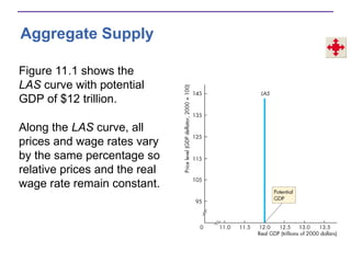
Figure 11.1shows the
LAS curve with potential
GDP of $12 trillion.
Along the LAS curve, all
prices and wage rates vary
by the same percentage so
relative prices and the real
wage rate remain constant.
9.
Aggregate Supply
Short-Run AggregateSupply
Short-run aggregate supply is the relationship between
the quantity of real GDP supplied and the price level when
the money wage rate, the prices of other resources, and
potential GDP remain constant.
A rise in the price level with no change in the money wage
rate and other factor prices increases the quantity of real
GDP supplied.
The short-run aggregate supply curve (SAS) is upward
sloping.
10.
Aggregate Supply
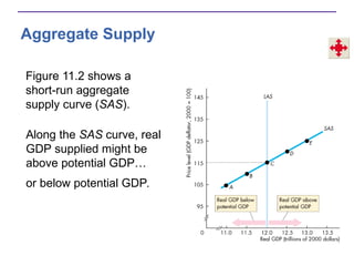
Figure 11.2shows a
short-run aggregate
supply curve (SAS).
Along the SAS curve, real
GDP supplied might be
above potential GDP…
or below potential GDP.
11.
Aggregate Supply
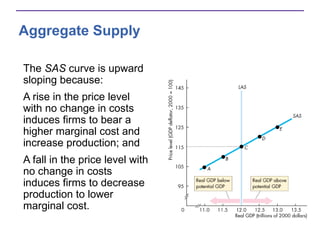
The SAScurve is upward
sloping because:
A rise in the price level
with no change in costs
induces firms to bear a
higher marginal cost and
increase production; and
A fall in the price level with
no change in costs
induces firms to decrease
production to lower
marginal cost.
12.
Aggregate Supply
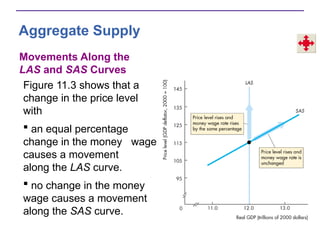
Movements Alongthe
LAS and SAS Curves
Figure 11.3 shows that a
change in the price level
with
an equal percentage
change in the money wage
causes a movement
along the LAS curve.
no change in the money
wage causes a movement
along the SAS curve.
13.
Aggregate Supply
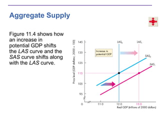
Changes inAggregate Supply
When potential GDP increases, both the LAS and SAS
curves shift rightward.
Potential GDP changes, for three reasons:
The full-employment quantity of labor changes
The quantity of capital (physical or human) changes
Technology advances
14.
Aggregate Supply
Figure 11.4shows how
an increase in
potential GDP shifts
the LAS curve and the
SAS curve shifts along
with the LAS curve.
15.
Aggregate Supply
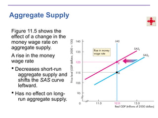
Figure 11.5shows the
effect of a change in the
money wage rate on
aggregate supply.
A rise in the money
wage rate
Decreases short-run
aggregate supply and
shifts the SAS curve
leftward.
Has no effect on long-
run aggregate supply.
16.
Aggregate Demand
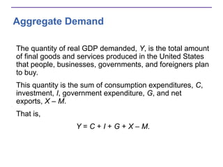
The quantityof real GDP demanded, Y, is the total amount
of final goods and services produced in the United States
that people, businesses, governments, and foreigners plan
to buy.
This quantity is the sum of consumption expenditures, C,
investment, I, government expenditure, G, and net
exports, X – M.
That is,
Y = C + I + G + X – M.
17.
Aggregate Demand
Buying plansdepend on many factors and some of the
main ones are
The price level
Expectations
Fiscal policy and monetary policy
The world economy
18.
Aggregate Demand
The AggregateDemand Curve
Aggregate demand is the relationship between the
quantity of real GDP demanded and the price level.
The aggregate demand curve (AD) plots the quantity of
real GDP demanded against the price level.
19.
Aggregate Demand
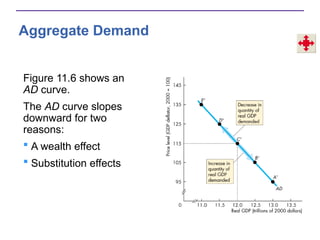
Figure 11.6shows an
AD curve.
The AD curve slopes
downward for two
reasons:
A wealth effect
Substitution effects
20.
Aggregate Demand
Wealth Effect
Arise in the price level, other things remaining the same,
decreases the quantity of real wealth (money, stocks, etc.).
To restore their real wealth, people increase saving and
decrease spending, so the quantity of real GDP demanded
decreases.
Similarly, a fall in the price level, other things remaining the
same, increases the quantity of real wealth.
With more real wealth, people decrease saving and
increase spending, so the quantity of real GDP demanded
increases.
21.
Aggregate Demand
Substitution Effects
1.Intertemporal substitution effect:
A rise in the price level, other things remaining the same,
decreases the real value of money and raises the interest
rate.
When the interest rate rises, people borrow and spend
less so the quantity of real GDP demanded decreases.
Similarly, a fall in the price level increases the real value of
money and lowers the interest rate.
When the interest rate falls, people borrow and spend
more so the quantity of real GDP demanded increases.
22.
Aggregate Demand
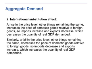
2. Internationalsubstitution effect:
A rise in the price level, other things remaining the same,
increases the price of domestic goods relative to foreign
goods, so imports increase and exports decrease, which
decreases the quantity of real GDP demanded.
Similarly, a fall in the price level, other things remaining
the same, decreases the price of domestic goods relative
to foreign goods, so imports decrease and exports
increase, which increases the quantity of real GDP
demanded.
23.
Aggregate Demand
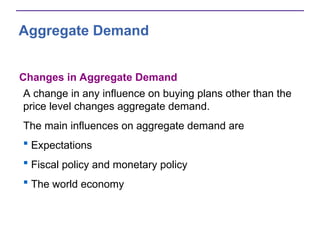
Changes inAggregate Demand
A change in any influence on buying plans other than the
price level changes aggregate demand.
The main influences on aggregate demand are
Expectations
Fiscal policy and monetary policy
The world economy
24.
Aggregate Demand
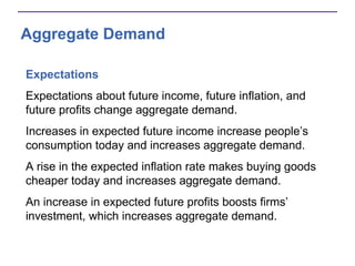
Expectations
Expectations aboutfuture income, future inflation, and
future profits change aggregate demand.
Increases in expected future income increase people’s
consumption today and increases aggregate demand.
A rise in the expected inflation rate makes buying goods
cheaper today and increases aggregate demand.
An increase in expected future profits boosts firms’
investment, which increases aggregate demand.
25.
Aggregate Demand
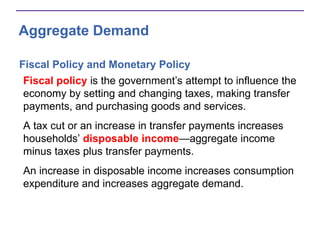
Fiscal Policyand Monetary Policy
Fiscal policy is the government’s attempt to influence the
economy by setting and changing taxes, making transfer
payments, and purchasing goods and services.
A tax cut or an increase in transfer payments increases
households’ disposable income—aggregate income
minus taxes plus transfer payments.
An increase in disposable income increases consumption
expenditure and increases aggregate demand.
26.
Aggregate Demand
Fiscal Policyand Monetary Policy
Because government expenditure on goods and services
is one component of aggregate demand, an increase in
government expenditure increases aggregate demand.
Monetary policy is changes in interest rates and the
quantity of money in the economy.
An increase in the quantity of money increases buying
power and increases aggregate demand.
A cut in interest rates increases expenditure and increases
aggregate demand.
27.
Aggregate Demand
The WorldEconomy
The world economy influences aggregate demand in two
ways:
A fall in the foreign exchange rate lowers the price of
domestic goods and services relative to foreign goods and
services, increases exports, decreases imports, and
increases aggregate demand.
An increase in foreign income increases the demand for
U.S. exports and increases aggregate demand.
28.
Aggregate Demand
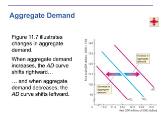
Figure 11.7illustrates
changes in aggregate
demand.
When aggregate demand
increases, the AD curve
shifts rightward…
… and when aggregate
demand decreases, the
AD curve shifts leftward.
29.
Macroeconomic Equilibrium
Short-Run MacroeconomicEquilibrium
Short-run macroeconomic equilibrium occurs when the
quantity of real GDP demanded equals the quantity of real
GDP supplied at the point of intersection of the AD curve
and the SAS curve.
30.
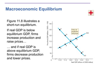
Macroeconomic Equilibrium
Figure 11.8illustrates a
short-run equilibrium.
If real GDP is below
equilibrium GDP, firms
increase production and
raise prices…
… and if real GDP is
above equilibrium GDP,
firms decrease production
and lower prices.
31.
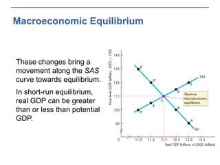
Macroeconomic Equilibrium
These changesbring a
movement along the SAS
curve towards equilibrium.
In short-run equilibrium,
real GDP can be greater
than or less than potential
GDP.
32.
Macroeconomic Equilibrium
Long-Run MacroeconomicEquilibrium
Long-run macroeconomic equilibrium occurs when real
GDP equals potential GDP—when the economy is on its
LAS curve.
Long-run equilibrium occurs at the intersection of the AD
and LAS curves.
33.
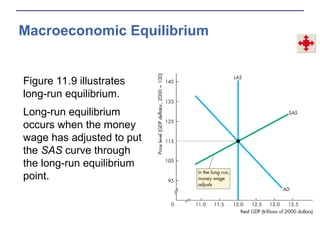
Macroeconomic Equilibrium
Figure 11.9illustrates
long-run equilibrium.
Long-run equilibrium
occurs when the money
wage has adjusted to put
the SAS curve through
the long-run equilibrium
point.
34.
Macroeconomic Equilibrium
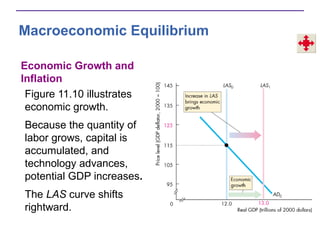
Economic Growthand
Inflation
Figure 11.10 illustrates
economic growth.
Because the quantity of
labor grows, capital is
accumulated, and
technology advances,
potential GDP increases.
The LAS curve shifts
rightward.
35.
Macroeconomic Equilibrium
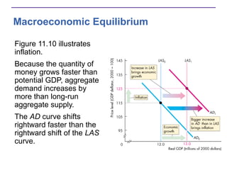
Figure 11.10illustrates
inflation.
Because the quantity of
money grows faster than
potential GDP, aggregate
demand increases by
more than long-run
aggregate supply.
The AD curve shifts
rightward faster than the
rightward shift of the LAS
curve.
36.
Macroeconomic Equilibrium
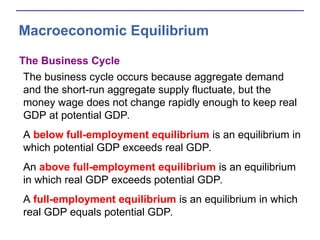
The BusinessCycle
The business cycle occurs because aggregate demand
and the short-run aggregate supply fluctuate, but the
money wage does not change rapidly enough to keep real
GDP at potential GDP.
A below full-employment equilibrium is an equilibrium in
which potential GDP exceeds real GDP.
An above full-employment equilibrium is an equilibrium
in which real GDP exceeds potential GDP.
A full-employment equilibrium is an equilibrium in which
real GDP equals potential GDP.
37.
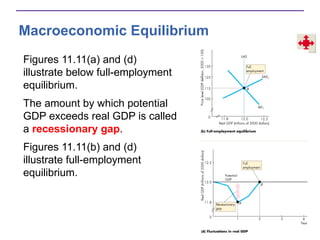
Macroeconomic Equilibrium
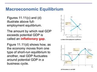
Figures 11.11(a)and (d)
illustrate below full-employment
equilibrium.
The amount by which potential
GDP exceeds real GDP is called
a recessionary gap.
Figures 11.11(b) and (d)
illustrate full-employment
equilibrium.
38.
Macroeconomic Equilibrium
Figures 11.11(c)and (d)
illustrate above full-
employment equilibrium.
The amount by which real GDP
exceeds potential GDP is
called an inflationary gap.
Figure 11.11(d) shows how, as
the economy moves from one
type of short-run equilibrium to
another, real GDP fluctuates
around potential GDP in a
business cycle.
39.
Macroeconomic Equilibrium
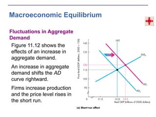
Fluctuations inAggregate
Demand
Figure 11.12 shows the
effects of an increase in
aggregate demand.
An increase in aggregate
demand shifts the AD
curve rightward.
Firms increase production
and the price level rises in
the short run.
40.
Macroeconomic Equilibrium
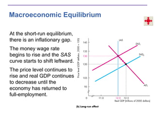
At theshort-run equilibrium,
there is an inflationary gap.
The money wage rate
begins to rise and the SAS
curve starts to shift leftward.
The price level continues to
rise and real GDP continues
to decrease until the
economy has returned to
full-employment.
41.
Macroeconomic Equilibrium
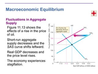
Fluctuations inAggregate
Supply
Figure 11.13 shows the
effects of a rise in the price
of oil.
Short-run aggregate
supply decreases and the
SAS curve shifts leftward.
Real GDP decreases and
the price level rises.
The economy experiences
stagflation.
42.
Macroeconomic Schools ofThought
Macroeconomists can be divided into three broad schools
of thought:
Classical
Keynesian
Monetarist
43.
Macroeconomic Schools ofThought
The Classical View
A classical macroeconomist believes that the economy
is self-regulating and always at full employment.
The term “classical” derives from the name of the
founding school of economics that includes Adam Smith,
David Ricardo, and John Stuart Mill.
A new classical view is that business cycle fluctuations
are the efficient responses of a well-functioning market
economy that is bombarded by shocks that arise from
the uneven pace of technological change.
44.
Macroeconomic Schools ofThought
The Keynesian View
A Keynesian macroeconomist believes that left alone, the
economy would rarely operate at full employment and that
to achieve and maintain full employment, active help from
fiscal policy and monetary policy is required.
The term “Keynesian” derives from the name of one of the
twentieth century’s most famous economists, John
Maynard Keynes.
A new Keynesian view holds that not only is the money
wage rate sticky but also are the prices of goods sticky.
45.
Macroeconomic Schools ofThought
The Monetarist View
A monetarist is a macroeconomist who believes that the
economy is self-regulating and that it will normally
operate at full employment, provided that monetary
policy is not erratic and that the pace of money growth is
kept steady.
The term “monetarist” was coined by an outstanding
twentieth-century economist, Karl Brunner, to describe
his own views and those of Milton Friedman.
#1 Notes and teaching tips: 7, 13, 21, 36, 40, and 50.
To view a full-screen figure during a class, click the red “expand” button.
To return to the previous slide, click the red “shrink” button.
To advance to the next slide, click anywhere on the full screen figure.
#7 The flavor of the Classical-Keynesian controversy. The textbook presents mainstream macroeconomics and does not dwell on controversy. But if you want to convey the flavor of the Classical-Keynesian controversy, you can do so now using the aggregate supply curves. The difference between the upward-sloping SAS and the vertical LAS curve lies at the core of the disagreement between Classical economists who believe that wages and prices are highly flexible and adjust rapidly and Keynesian economists who believe that the money wage rate in particular adjusts very slowly.
Along the LAS curve—two things happening. Students seem comfortable with the idea that the SAS curve has a positive slope; but they seem less at ease with the vertical LAS curve. Emphasize (as the textbook does) the crucial idea that along the LAS curve two sets of prices are changing — the prices of output and the prices of resources, especially the money wage rate. Once they get this point, students quickly catch on to the result that firms won’t be motivated to change their production levels along the LAS curve. The vertical LAS curve is both vital and difficult and class time spent on this concept is well justified.
#13 One LAS curve, but many SAS curves. Another way of reinforcing the distinction between the two AS curves is to point out to students that, at any given time, there is just one LAS curve, corresponding to potential GDP. But there is an infinite number of possible SAS curves, each corresponding to a different money wage rate.
#21 Keep it simple. You know that the AD curve is a subtle object—an equilibrium relationship derived from simultaneous equilibrium in the goods market and the money market. This description of the AD curve is not helpful to students in the principles course and is a topic for the intermediate macro course. At the same time that we want to simplify the AD story, we also want to avoid being misleading. The textbook walks that fine line, and we suggest that you stick closely to the textbook treatment and don’t try to convey the more subtle aspects of AD.
Not a strict ceteris paribus event. A major problem with the AD curve is that a change in the price level that brings a movement along the curve is not a strict ceteris paribus event. A change in the price level changes the quantity of real money, which changes the interest rate. Indeed, this chain of events is one of the reasons for the negative slope of the AD curve. In telling this story, we must be sensitive to the fact that the student doesn’t yet know about the demand for money. We must provide intuition with stories (like the Maria stories in the textbook) without referring to the demand for money.
Income equals expenditure on the AD curve. Some instructors want to emphasize a second and more subtle violation of ceteris paribus, that along the AD curve, aggregate planned expenditure equals real GDP. That is, the AD curve is not drawn for a given level of income but for the varying level of income that equals the level of planned expenditure. If you want to make this point when you first introduce the AD curve, you must cover the AE model of Chapter 23 before you cover this chapter. (The material is written in a way that permits this change of order.) If you do not want to derive the AD curve from the equilibrium of the AE model, don’t even mention what’s going on with income along the AD curve. Silence is vastly better than confusion. You can pull this rabbit out of the hat when you get to Chapter 23 if you’re covering that material.
#36 Short-run macroeconomic equilibrium. Emphasize that in short-run macroeconomic equilibrium, firms are producing the quantities that maximize profit and everyone is spending the amount that they want to spend. Describe the convergence process using the mechanism laid out on page 516 of the textbook. In that process, firms always produce the profit-maximizing quantities—the economy is on the SAS curve. If they can’t sell everything they produce, firms lower prices and cut production. Similarly, if they can’t keep up with sales and inventories are falling, firms raise prices and increase production. These adjustment processes continues until firms are selling their profit-maximizing output. Emphasize also that with a fixed (sticky) money wage rate, this short-run equilibrium can be at, below, or above potential GDP.
#40 Long-run macroeconomic equilibrium. You can use the idea that there is only one LAS curve-but many SAS curves to explain long-run equilibrium. In long-run equilibrium, real GDP equals potential GDP on the one LAS curve. The money wage rate is at the level that makes the SAS curve the one of the infinite number of possible SAS curves that passes through the intersection of AD and LAS curves.
From the short run to the long run. Explain that market forces move the money wage rate to the long-run equilibrium level. At money wage rates below the long-run equilibrium level, there is a shortage of labor, so the money wage rate rises. At money wage rates above the long-run equilibrium level, there is a surplus of labor, so the money wage rate falls. At the long-run equilibrium money wage rate, there is neither a shortage nor a surplus of labor and the money wage rate remains constant.
Shifting the SAS curve. Reinforce the movement toward long-run equilibrium with a curve-shifting exercise. Take the case where the AD curve shifts rightward. The fact that the initial equilibrium occurs where the new AD curve intersects the SAS curve is not difficult. But the notion that the SAS curve shifts leftward as time passes is difficult for many students. The trick to making this idea clear is to spend enough time when initially discussing the SAS so that the students realize that wages and other input prices remain constant along an SAS curve. Once the students see this point, they can understand that, as input prices increase in response to the higher level of (output) prices, the SAS curve shifts leftward.
Avoid confusing students by using ‘up’ to correspond to a decrease in SAS. But do point out that that when the SAS curve shifts leftward it is moving vertically upward, as input prices rise to become consistent with potential GDP and the new long-run equilibrium price level. Most students find it easier to see why the SAS curve shifts leftward once they see that rising input prices shift the curve vertically upward.
#50 Putting the AS-AD model to work. Don’t neglect the predictions of the model. This is the payoff for the student. With this simple model, we can now say quite a lot about growth, inflation, and the cycle.
The price level doesn’t fall, and real GDP rarely falls. The AS-AD model predicts a fall in the price level when either aggregate demand decreases or aggregate supply increases. And the model predicts that real GDP decreases when either aggregate supply or aggregate demand decreases. Students are sometimes bothered by this apparent mismatch between the predictions of the model and the observed economy. The best way to handle this issue is to emphasize that in our actual economy, AS and AD almost always are increasing. When we use the model to simulate the effects of a decrease in either AS or AD, we’re studying what happens relative to the trends in real GDP and the price level. A fall in the price level in the model translates into a lower price level than would otherwise have occurred and a slowing of inflation. The story is similar for real GDP.