HMM-Based Speech Synthesis

International Journal of Modern Engineering Research (IJMER)
www.ijmer.com Vol.3, Issue.4, Jul - Aug. 2013 pp-1894-1899 ISSN: 2249-6645
www.ijmer.com 1894 | Page
Smita Chopde#
, Pushpa U. S.*
#
EXTC Dept. Mumbai University, Mumbai
Abstract: This paper describes a approach to text-to-speech synthesis (TTS) based on HMM. In the proposing approach,
speech spectral parameter sequences are generated from HMMs directly based on maximum likelihood criterion. By
considering relationship between static and dynamic features during parameter generation, smooth spectral sequences are
generated according to the statistics of static and dynamic parameters modelled by HMMs, resulting in natural sounding
speech. In this paper, first, the algorithm for parameter generation is derived, and then the basic structure of an HMM based
TTS system is described. Results of subjective experiments show the effectiveness of dynamic feature.
Keywords: Include at least 5 keywords or phrases
I. INTRODUCTION
A Hidden Markov Model (HMM) is finite state machine which generates a sequence of discrete time observation.
At each time unit (frame) the HMM changes state according to state transition probability distribution, and then generates an
observation ot at time t according to output probability distribution of the current state .Hence the HMM is doubly stochastic
random process model.
An N state HMM is defined by state transition probability distribution A= 𝑎𝑖𝑗 𝑁 𝑖, 𝑗 = 0and output probability
B={bj(o)}N
j=0 and initial state probability distribution π= {πi}N
i=0 . For convenience the compact notation.
λ =(A,B,π)
Figure 1. Examples of HMM parameter is used to indicate parameter set of the model
Figure 1 shows the HMM model Figure 1 (a) shows the 3 state ergodic state ,in every state of model could be
reached from every other state of the model in single step figure 1(b) shows the a 3 state left to right model in which the
state index increases or stays same as time increase. Generally left to right HMMs are used to model speech parameter
sequence since they can appropriate model signal whose property changes in successive manner. The output probability
distribution bj(ot) can be discrete or continuous depending on the observation. Usually in continuous distribution HMM
(CDHMM) an output probability distribution is modelled by mixture of multivariate Gaussian distribution which as follows
M
bj(o)= ∑wjmN(o|µjm,,Ujm)
m=1
Where M= number of mixture component wjm, μjm, Ujm are weight, a mean vector, and covariance matrix component m
of state j, respectively. A Gaussian distribution N (o|µjm,,Ujm) is defined by
N(o|µjm,,Ujm) = ( 1/( 2𝜋 )d
|𝑈|) exp⁡(−1/2(𝑜 − µµjm)Τ
Ujm
-1
(o - µjm)
Where d is dimensionality of o. mixture weight wjm satisfies the stochastic constraint
∑wjm =1 1≤ j≤ N
Wjm ≥ 0 1≤ j≤ N, 1≤ m ≤ M
So that bj(o) are properly normalized .
ᶋ 𝑏𝑗 𝑜 𝑑𝑜 = 1 1≤ j≤ N
When the observation vector o is divided into S independent data stream i.e. o = [o1
Τ
,o2
Τ
, o3
Τ
,....................oS
Τ
]Τ
bj(o) is
formulated by product of Gaussian mixture densities.
S
bj(o)=Π bjs(os)
s=1
HMM-Based Speech Synthesis

S Ms
bj(o)= Π{ΠwjsmN(os|µjsm,Ujsm )}
s=1 m=1
Likelihood calculation
When the state sequence is determined as Q= (q1 q2 q3 q 4….qT ), the likelihood of generating an observation sequence
O=(o1, o2, o3, o4,….oT) is calculated by multiplying the state transition probabilities and output probabilities for each state
𝑃 𝑂,
𝑄
𝜆
= 𝑨𝒒𝒕 − 𝟏, 𝑨𝒒𝒕, 𝑩𝒒𝒕, 𝑶 𝒕
𝑻
𝒕=𝟏
Where Aq0j denote πj. The likelihood of generating O from HMM 𝞴 is calculated by summing P(O,Q/𝞴) for all possible
sequences
𝑃
𝑜
𝞴
= 𝑨𝒒𝒕 − 𝟏, 𝑨𝒒𝒕, 𝑩𝒒𝒕, 𝑶(𝒕)
𝑻
𝒕=𝟏𝑸𝒂𝒍𝒍
The likelihood of above equation is sufficiently calculated using forward and/or backward procedure .
The forward and backward variables are
αt(i)=P(o1,o2,...........oT,qt=i/λ)
βt(i)=P(ot+1 ,ot+2, ...................oT,q=i,λ)
can be calculated individually as
1. Initialization
α1(i)=Π bi(o1) 1<i<N
βT (i) = 1 1<i<N`
2. Recursion
αT+1(i)= αt (j)aji𝑁
𝑗=1 𝑏i(t+1) 1 <i<N
t=2,.....................T
3. Termination
P* =max[(δT(i) ]
q*=argmax[(δT(i) ]
4. Path back tracking
qt
*
= Ψt+1(q*
t+1)
Maximum Likelihood Estimation of HMM parameter
There is no known method to analytically obtain the model parameter set based on maximum likelihood based on
maximum likelihood (ML) criterion ., that is to obtain which maximises likelihood P(O/λ) for a given observation
sequence O , in a closed form. Since this problem is a high dimensional nonlinear optimization problem, and there will be
number of local maxima . , it is difficult to obtain λ which globally maximizes P(O/λ) and can be obtained using an
iterative procedure such as the expectation –maximization (EM) algorithm ( which is often referred to as Baum-Weich
algorithm), and the obtained parameter set will be a good estimate if a good initial estimate is provided .
In the following , the EM algorithm for the CD-HMM are described . The algorithm for the HMM with discrete output
distribution can also be derived in the straight forward manner
Q-Function
In the E M algorithm , an auxiliary function Q(λ’,λ) of current parameter set λ’ and new parameter set λ is defined
as follows
Q(λ’,λ)=
1
𝑃(
𝑂
𝜆
)
𝑃 𝑂, 𝑄 𝜆′
logP(O, Qλ).
Here , each mixture component is decomposed into a substrate and Q is redefined as a substrate sequence i.e.
Q=((q1 ,s1) ,(q2 ,s2 ), ......................(qT,sT)
Where (qT,sT) represents the being substrate st of state qt at time t.
At each iteration of procedure current parameter set λ’ is replace by new parameter set which maximises Q(λ’,λ).
This iterative procedure can be provided to increase likelihood P(O|λ) monotonically and converge to a certain critical
point since it can provide that Q- function satisfies the following theorem
Theorem 1
Q(λ’,λ)≥ Q(λ’,λ’) i.e. P(O|λ)≥P(O|λ’)
Theorem 2
The auxiliary function Q(λ’,λ) has a unique global maximum as a function of λ and this is the one and the critical point.
Theorem 3
A parameter set λ is the critical point of the likelihood P(O|λ) if and only if it is a critical point of the Q- function.
Maximization of the Q-Function
logP(O, O|λ) can be written as
logP(O, O|λ)= 𝑎𝑞𝑡 − 1𝑞𝑡𝑇
𝑡=1 + 𝑤𝑞𝑡𝑠𝑡𝑇
𝑡=1 + log⁡(𝒩 (𝑜𝑡|µ𝑞𝑡 𝑠𝑡,Uqt st),
where aq0q1 denotes Πq1. Hence the Q function can be written as

Q(λ’,λ)= 𝑃(𝑂, 𝑞1 = 𝑖|𝑁
𝑖=1 λ’)logΠi
+ 𝑃 𝑂, 𝑞𝑡 = 𝑖, 𝑞𝑡 + 1 = 𝑗 𝜆′
𝑙𝑜𝑔𝑎𝑖𝑗𝑇−1
𝑡=1
𝑁
𝑗=1
𝑁
𝑖=1 + 𝑃 𝑂, 𝑞𝑡 = 𝑖, 𝑠𝑡 = 𝑘 𝜆′
𝑙𝑜𝑔𝑤𝑞𝑡𝑠𝑡𝑇
𝑡=1
𝑁
𝑗 =1
𝑁
𝑖=1 +
𝑃 𝑂, 𝑞𝑡 = 1, 𝑠𝑡 = 𝑘 𝜆 𝑙𝑜𝑔𝒩(𝑜𝑡|µ𝑞𝑡𝑠𝑡, 𝑈𝑞𝑡𝑠𝑡𝑇
𝑡=1
𝑀
𝑘=1
𝑁
𝑖=1 )
𝛱𝑖 = 1
𝑁
𝑖=1
𝑎𝑖𝑗 = 1𝑁
𝐽=1 1≤i≤N
𝑤𝑖𝑘 = 1𝑀
𝑘=1 1≤i≤N
can be derived from lagaranges or differential calculs.
Πi = γ1(i), aij=
𝜉′ 𝑡(𝑖,𝑗)𝑇−1
𝑡=1
𝛾𝑡 (𝑖)𝑇−1
𝑡=1
; 𝑤𝑖𝑘 =
𝛾𝑡 (𝑖,𝑘 )𝑇
𝑡−1
𝛾𝑡(𝑖)𝑇
𝑡−1
; µ𝑖𝑘 =
𝛾𝑡 𝑖,𝑘 .𝑂𝑡𝑇
𝑡−1
𝛾𝑡 (𝑖,𝑘)𝑇
𝑡=1
; 𝑈𝑖𝑘 =
𝛾𝑡 𝑖,𝑘 . 𝑜𝑡− µ𝑖𝑘 .(𝑜𝑡− µ𝑖𝑘)𝑇
𝑡−1
𝛾𝑡 (𝑖,𝑘)𝑇
𝑡−1
Probability of state i being at t and probability of state i being at t+1 are
𝛾𝑡 𝑖 = 𝑃 𝑂, 𝑞𝑡 = 𝑖 𝜆 =
𝛼𝑖 𝑡 𝛽𝑡 (𝑖)
𝛼𝑡 𝑗 𝛽𝑡 (𝑗)𝑁
𝑗=1
; γt(i,k)=P(O,qt=1,st=k|λ)=
𝛼𝑡 𝑖 𝛽𝑡 (𝑖)
𝛼𝑡 𝑗 𝛽𝑡 (𝑗)𝑁
𝑗=1
.
𝑤𝑗𝑘𝒩 (𝑜𝑡|µ𝑗𝑘 ,𝑈𝑗𝑘 )
𝑤𝑗𝑚𝒩 (𝑜𝑡|µ𝑗 𝑚′ 𝑈𝑗𝑚 )𝑀
𝑚 =1
ξt(i,j)=P(O,qt=i,qt+1=j|λ)=
𝛼𝑡 𝑖 𝑏𝑗 𝑜𝑡+1 𝛽𝑡 +1(𝑗 )
𝛼𝑡 𝑙 𝛼𝑙𝑛𝑏𝑛 𝑜𝑡+1 𝛽𝑡 +1(𝑛)𝑁
𝑛=1
𝑁
𝑡=1
II. METHOD
The system consists of two stages : the training stage and the synthesis stage.First in training stage mel-cepstrumm
coffecient are obtained from the speech signal by delta –delta mel-cepstral coefficient.Then phoneme HMM are trained
using mel-cepstral coefficient and their deltas and deltas-deltas .
In the synthesis stage an arbitrary given text to be synthesized is transformed into phoneme sequence . According
to phoneme sequence , a sentence HMM which represents the whole text to be synthesized is constructed by concatening
phoneme HMMs. From the sentence HMM ,a speech parameter is generated using the algorithm for speech parameter
generation for HMM By using Mel-Log spectral Approximation speech is synthesized from the generated mel-spectral
coefficient.
Speech data base
HMM are trained using 503 phonetically balance sentences uttered by male speaker . Speech signal is sampled at
20KHz and downsampled to 10KHz and re-labelled using 60 phonemes and silence given in table 1. Unvoiced vowles
with previous consonants are treated as individual phonemes e.g shi is composed of unvoiced i with previous sh.
Vowels
a , i, u,e,o
Consonants
N, m , n ,y,w,r,p,pp,t,tt,k,kk,b,d,dd,
g, ch cch ts tts s ss sh, ssh, h,f ,ff,z
j, my ny ry by gyp y ppy ky kky hy
Unvoiced vowels with previous consonants
pi, pu,ppi,ki,ku,kku,chi,cchi,tsu,su,shi,
shu, sshi,sshu, hi, fu
Table :1 Phoenems used in system
Figure:2 Block diagram of HMM based speech synthesis system.
Speech Analysis
Speech signal are windowed by 25.6ms Blackman window with 5ms shift , then mel cepstral coefficients are obtained by
15 th order mel-cepstral analysis. The dynamic feature Δct and ΔΔct i.e. delta and delta –delta mel-cepstral coefficient at
frame t are calculated as
Δct =
1
2
(ct+1 – ct-1), Δ2
ct =
1
2
(Δct+1 - Δct-1)
The feature vector is composed of 16 mel- cepstral coefficient including the zeroth coefficient and their delta and delta-
delta coefficient .

Training of HMM
All HMM used in system were left- to – right model with no skip . each state has single Gaussian distribution with
diagonal convergence . Initially a set of microphone models were trained . These models were cloned to produce a triphone
model for all distinct triphones in the training data. The triphone models were reestimated with the embedded version of
Bauman Welch version algorithm. All the states at same position of the triphone HMM derived from same microphone
HMM were clustered using further neighbourhood hierarchical clustering algorithm. The output distribution in the same
cluster were tied to reduce the number of parameters and to balance the complexity against the available data .Tied
triphone models were re estimated with embedded training again.
Finally the data was aligned to the models via viterbi algorithm to obtain state duration densities . each of the state duration
densities was modelled by single Gaussian distribution .
Speech Synthesis
An aritbitrary given text to be synthesized is converted in phoneme sequence Then triphone HMM corresponding to
the phoneme sequence are concatenated to obtain HMM sentence which represents the whole text to be synthesized .
Instead of triphones which did not exist in the training data , monophone models are used .. From the sentence HMM , a
speech parameter sequence is generated using algorithm. By using MLSA filter speech is synthesized from the generated
mel cepstral coefficient directly .
Subjective Experiments
Subjective test were conducted to evaluate the effect of including dynamic feature and to investigate the
relationship between the number of states of tied triphone HMMs and the quality of speech synthesized .The test sentence
consisted of twelve sentences which were not included in training sentences. Fundamental frequency contours were
extracted from natural utterances, and used for speech synthesis using linear time warping within each phoneme to adjust
phoneme duration of extracted fundamental frequency contours to generated parameter sequence . In the test sentences set,
there exist 619 distinct triphonens in which 38(5.8%) triphones where not included in training data and replaced by
monophones. The test sentence set where divided into three set and each set was evaluated by individual subjects . Subjects
were presented with a pair of synthesized set at each trial, and asked to judge which of two speech samples sounded better
.
Effect of dynamic features
To investigate the effect of dynamic features , a pared compression test was conducted . Speech samples used in the
test were synthesized using (1) speech spectral sequence generated without dynamic feature from model stringed using
static features
(2) spectral sequence generated using only static features and then linearly interpolated between the centers of state
duration.
(3) Spectral sequence generated using static and delta parameters from the models trained using static and dynamic
parameter
(4) Spectral parameters generated using static , delta and delta –delta from the models trained using static, delta and delts-
delta parameters. All the models were triphone models without sate tying.
Figure:3 Effects of dynamic features
Figure:3 shows the results of the paired comparison test. Vertical axis denotes the preference score . From the result it can be
seen that the score for synthetic speech generated using dynamic feature are much higher than those synthetics speech
generated using static features with and without linear interpolation. This is due that by exploiting statics of dynamic features
for speech parameter generation, generated spectral sequence can reflect not only shapes spectra but also transition
appropriately comparing to spectral sequence generated using static features only with linear interpolation.
State tying
To investigate the relationship between total number of state of tied tri phone HMMs and quality of speech
synthesized speech, paired comparison test were conducted using 3 and 5 tied triphone HMMs .By modifying stop character
for state clustering several sets of HMMs which had different numbers of states were prepared for test. For 3-stse HMMs
comparison were performed using triphone model without state tying(totally 10,544 states ) tied triphone models with totally
1,961and 1,222 states and monophone models (183 states) and for 5 state HMMs triphone models without state tying
0.00%
20.00%
40.00%
60.00%
80.00%
100.00%
Series1

(totally 17,590 states ), tied triphone models with totaly 2,040 and 1,199 states and monophone models (305 states). It is
noted that sate duration distribution of triphone models were also used for monophone models to avoid of phoneme duration
on speech quality.
Figure: 4a 3 state HMMs
Figure:4b 5 state model
Figure: 4a and Figure:4b shows the result for 3 state and 5 state HMM. From the result , it can be seen that the quality of
synthetic speech degrade as the number of states decrease .From informal listening test and investigation of generated
spectra , it was observed that shapes of spectra were getting flatten as the number of state decreases and this cause
degrading of in intelligibility . It was observed that that the audible discontinuity in synthetic speech increased as the
number of state increased , meanwhile the generated spectra varied smoothly when the number of states were small. The
discontinuity caused in the lower score for 5 state triphone models compared to 3 – state triphone models. It is noted that
significant degradation in communicability was not observed even if the mono phone models were used for speech
synthesis .
0.00%
10.00%
20.00%
30.00%
40.00%
50.00%
60.00%
70.00%
80.00%
90.00%
Series1
p
r
e
f
e
r
e
n
c
e
s
c
o
r
e%
0.00%
10.00%
20.00%
30.00%
40.00%
50.00%
60.00%
70.00%p
r
e
f
e
r
e
n
c
e
s
c
o
r
e
%

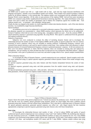
Figure: 5 Comparison of 3-state and 5- state HMMs
Along x-axis
1 3-state HMM (1961 states)
From the above figure it can be seen that scores for 3-state and 5-state models were almost equivalent when number of
states were almost 2000, the score of 5-state models was better when the number states were 1200. When the total number
of tied states were almost the same , 5- sate model has higher resolution in time than 3- sate model reversely, 3-sate model
has better resolution in parameter space than 5-state model .From the result if total number of state state is limited, models
with higher resolution in time can synthesize more naturally sounding speech than model with higher parameter resolution
in space .
III. CONCLUSION
In parameter generation algorithm a speech generation sequence is obtained so that likelyhood of HMM for
generated parameter sequence is maximized. By exploiting the constraints between static and dynamic features the
generated parameter sequence results not only for static of shapes of spectra but also transition obtained from training data
appropriately, resulting in smooth and realistic spectral sequence .In parameter generation algorithm a problem of
generating parameter speech was simplified assuming that parameter sequence was generated along single path. The
extended parameter algorithm using multi-mixture HMMs model has more ability to generate natural soundings speech,
however extended algorithm has more computational complexity since it is based on expectation- maximization algorithm
,which results in iteration of forward –backward algorithm and parameter generation algorithm.
References
[1]. R . E. Donowan and E.M.Eide,”The IBM Trainable Speech Synthesis System,” Proc . ICSLP-98 , 5,pp,1703 1706 , Dec 1998.
[2]. F.A.Falaschi ,M. Giustiniani and M. Verola , “ A Hidden Markov Model approach to speech synthesis , “ Proc. EUROSPEECH-89,
pp.187-190.sep.1989.
[3]. A. Gustiniani and P.Pierucci, “Phonetic ergodic HMM for speech synthesis,” Proc.EUROSPEECH-91,pp.349-352,sep1991.
[4]. M. Tonomura, T.Kosakaand S. Matsunaga, “Speaker adaptation based on transfer vector field smoothing using maximum a posterior
probability estimation,” Computer speech and Language , vol.10.n0.2pp.117-132,Apr.1996.
0
0.1
0.2
0.3
0.4
0.5
0.6
0.7
1 2 3 4 5 6

HMM-Based Speech Synthesis

Recommended

Recommended

More Related Content

What's hot

What's hot (20)

Viewers also liked

Viewers also liked (19)

Similar to HMM-Based Speech Synthesis

Similar to HMM-Based Speech Synthesis (20)

More from IJMER

More from IJMER (20)

Recently uploaded

Recently uploaded (20)

HMM-Based Speech Synthesis