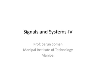
The document discusses Fourier representations of signals and linear time-invariant (LTI) systems. It begins by introducing Fourier series (FS) and Fourier transforms (FT) for continuous and discrete time periodic and non-periodic signals. It then provides examples of using Fourier series to represent continuous time periodic signals, including deriving FS coefficients and determining time domain signals from given FS coefficients. Key aspects covered are the FS representation as a weighted sum of complex sinusoids and interpretation of Fourier coefficients in the frequency domain.
This document discusses signals and systems from an introductory perspective. It defines a signal as a function that conveys information about a physical phenomenon, and can be one-dimensional or two-dimensional. A system is defined as an entity that manipulates signals to produce new signals. Application areas of signals and systems are discussed, including control, communications, and signal processing. Key concepts like continuous and discrete time signals, even and odd signals, periodic and non-periodic signals, and deterministic and random signals are introduced.
- The document discusses linear time-invariant (LTI) systems and their representations in the time domain.
- It covers various properties of LTI systems including parallel and cascade connections, causality, stability, and memory.
- Methods for representing LTI systems using impulse responses, differential/difference equations, and step responses are presented.
- Solving techniques for determining the homogeneous and particular solutions of LTI systems described by differential or difference equations are outlined.
Classification of signals
Deterministic and Random signals
Continuous time and discrete time signal
Even (symmetric) and Odd (Anti-symmetric) signal
Periodic and Aperiodic signal
Energy and Power signal
Causal and Non-causal signal
DSP_2018_FOEHU - Lec 03 - Discrete-Time Signals and SystemsAmr E. Mohamed
The document discusses discrete-time signals and systems. It defines discrete-time signals as sequences represented by x[n] and discusses important sequences like the unit sample, unit step, and periodic sequences. It then defines discrete-time systems as devices that take a discrete-time signal x(n) as input and produce another discrete-time signal y(n) as output. The document classifies systems as static vs. dynamic, time-invariant vs. time-varying, linear vs. nonlinear, and causal vs. noncausal. It provides examples to illustrate each classification.
Communication Systems_B.P. Lathi and Zhi Ding (Lecture No 22-30)Adnan Zafar
Lecture No 22: https://youtu.be/z3gia8eHEOo
Lecture No 23: https://youtu.be/tFZuaZ4i89I
Lecture No 24: https://youtu.be/BIcjuUxb6aE
Lecture No 25: https://youtu.be/ZPvO4CubmME
Lecture No 26: https://youtu.be/CxUWW4Uh5Gk
Lecture No 27: https://youtu.be/OZ2TwSXkeVw
Lecture No 28: https://youtu.be/HGYXtSvisRY
Lecture No 29: https://youtu.be/W1ehHa0AUnk
Lecture No 30: https://youtu.be/q5gh3tQ7aLk
control system Lab 01-introduction to transfer functionsnalan karunanayake
The document provides information about transfer functions and their characteristics including time response, frequency response, stability, and system order. It discusses different types of systems including first order and second order systems. It also demonstrates how to analyze transfer functions and obtain step and impulse responses using MATLAB. Key points include:
- Transfer functions relate the input and output of a system in the Laplace domain
- Time and frequency responses provide information about a system's behavior over time and at different frequencies
- Stability depends on the locations of the poles - systems are stable if all poles have negative real parts
- First and second order systems have distinguishing characteristics like rise time, settling time, overshoot
- MATLAB commands like step, impulse, pole can
The document discusses time domain analysis and standard test signals used to analyze dynamic systems. It describes the impulse, step, ramp, and parabolic signals which imitate characteristics of actual inputs such as sudden shock, sudden change, constant velocity, and constant acceleration. The time response of first order systems to these standard inputs is expressed mathematically. The impulse response directly provides the system transfer function. Step response reaches 63% of its final value within one time constant.
1. The document discusses operations that can be performed on continuous-time signals, including time reversal, time shifting, amplitude scaling, addition, multiplication, and time scaling.
2. It provides examples of each operation using the unit step function u(t) and illustrates the effect graphically. Combinations of operations are also demonstrated through examples.
3. Key operations include time shifting which delays a signal, time scaling which speeds up or slows down a signal, and their combination which first performs one operation and then the other.
VTU CBCS E&C 5th sem Information theory and coding(15EC54) Module -5 notesJayanth Dwijesh H P
This document provides information and formulas related to information theory and coding. It discusses important cyclic codes like Reed-Solomon codes and convolution codes. For convolution codes, it provides the generator matrix formulas in the time and transform domains, showing how the output of the encoder is calculated from the input and generator matrix. It also gives the formulas for calculating the output polynomials from the input polynomial and generator polynomials in the transform domain approach.
Dcs lec03 - z-analysis of discrete time control systemsAmr E. Mohamed
The document discusses discrete time control systems and their mathematical representation using z-transforms. It covers topics such as impulse sampling, the convolution integral method for obtaining the z-transform, properties of the z-transform, inverse z-transforms using long division and partial fractions, and mapping between the s-plane and z-plane. Examples are provided to illustrate various concepts around discrete time systems and their analysis using z-transforms.
This document contains lecture notes on signals and systems for a course at Chadalawada Ramanamma Engineering College. It includes:
1. An introduction to signals, systems, and some common elementary signals like the unit step, unit impulse, ramp, sinusoid, and exponential signals.
2. A classification of signals as continuous/discrete, deterministic/non-deterministic, even/odd, periodic/aperiodic, energy/power, and real/imaginary.
3. A discussion of basic operations on signals like amplitude scaling, addition, and subtraction.
The document discusses the benefits of exercise for mental health. Regular physical activity can help reduce anxiety and depression and improve mood and cognitive function. Exercise causes chemical changes in the brain that may help protect against mental illness and improve symptoms.
Spectral decomposition involves decomposing a matrix into its eigenvectors and eigenvalues. This decomposition has various applications including:
1. Decoupling linear differential equations by transforming the system into independent equations involving only single state variables.
2. Dimensionality reduction by projecting the data onto a lower dimensional subspace formed by the dominant eigenvectors, reducing the data size.
3. Filtering signals by removing components corresponding to unwanted eigenvalues/eigenvectors from the signal.
The key steps involve finding the eigenvalues and eigenvectors of the matrix using techniques like QR decomposition and back substitution, and then using the eigendecomposition to transform the original problem.
This document discusses linear and nonlinear systems. It defines a linear system as one that satisfies the principles of superposition and homogeneity or scaling. The principles of homogeneity and superposition for a linear system are defined. Homogeneity means that scaling the input scales the output by the same factor. Superposition means that the output for the sum of two inputs is the sum of the outputs for each input individually. A linear system thus satisfies the property of linearity, where the output of scaled and summed inputs is the scaled and summed outputs. Nonlinear systems do not satisfy these properties.
1. The document discusses signals and systems, including continuous-time and discrete-time signals. It covers topics like transformations of signals, exponential and sinusoidal signals, and basic properties of systems.
2. Continuous-time signals are represented as functions of time t, while discrete-time signals are represented as sequences indexed by integer n. Exponential and sinusoidal signals can be represented using complex exponential functions.
3. The document provides examples and formulas for calculating energy, power, and other properties of signals. It also describes how signals can be transformed through operations like time shifting, scaling, reversal, and periodicity.
This document contains the solutions to an homework assignment on linear and nonlinear systems. It examines several examples and determines whether they are linear or nonlinear by applying the superposition principle. It also identifies examples as causal or non-causal. Finally, it analyzes some circuit examples and determines properties like memoryless, causal, linear, and time-invariant.
The document discusses stable and unstable systems in control systems. It defines a stable system as one where the system response remains bounded for a bounded input. An unstable system is defined as one where the output diverges to infinity or becomes unbounded for a bounded input. Control system theory focuses on estimating the stability of systems as stability determines a system's applicability.
This document discusses time response specifications for second order systems, including delay time, rise time, peak time, and peak overshoot. It provides equations to calculate each specification based on the natural frequency (ωn) and damping ratio (δ) of the system. Rise time is defined as the time to rise from 10-90% of the final value and is calculated as (π - cos^-1δ)/ωn√(1-δ^2). Peak time is the time to reach the first peak and is calculated as π/ωn√(1-δ^2). Peak overshoot is calculated as 100e^(-δπ)/√(1-δ^2)
Chapter3 - Fourier Series Representation of Periodic SignalsAttaporn Ninsuwan
This document discusses Fourier series representation of periodic signals. It introduces continuous-time periodic signals and their representation as a linear combination of harmonically related complex exponentials. The coefficients in the Fourier series representation can be determined by multiplying both sides of the representation by complex exponentials and integrating over one period. The key steps are: 1) multiplying both sides by e-jω0t, 2) integrating both sides from 0 to T=2π/ω0, and 3) using the fact that the integral equals T when k=n and 0 otherwise to obtain an expression for the coefficients an. Examples are provided to illustrate these concepts.
DSP_FOEHU - Lec 08 - The Discrete Fourier TransformAmr E. Mohamed
The document discusses the Discrete Fourier Transform (DFT). It explains that while the discrete-time Fourier transform (DTFT) and z-transform are not numerically computable, the DFT avoids this issue. The DFT represents periodic sequences as a sum of complex exponentials with frequencies that are integer multiples of the fundamental frequency. It can be viewed as computing samples of the DTFT or z-transform at discrete frequency points, allowing numerical computation. The DFT provides a link between the time and frequency domain representations of a finite-length sequence.
Chapter 7 Controls Systems Analysis and Design by the frequency response analysis . From the book (Ogata Modern Control Engineering 5th).
7-1 introduction.
7-2 Bode diagrams.
This document provides an overview of adaptive filtering techniques. It discusses digital filters and classifications such as linear/nonlinear and finite impulse response (FIR)/infinite impulse response (IIR). It then covers Wiener filters, including how they minimize mean square error. The method of steepest descent is presented as an approach to solve the Wiener-Hopf equations to find optimal filter weights. Finally, it discusses how the least mean squares (LMS) algorithm can be used for adaptive filtering by updating filter weights recursively in the direction that reduces mean square error.
EC8352- Signals and Systems - Unit 2 - Fourier transformNimithaSoman
This document discusses Fourier transforms and their applications. It begins by introducing Fourier transforms and noting that they are used widely in optics, image processing, speech processing, and medical signal processing. It then covers key topics such as:
- When periodic and aperiodic signals can be represented by Fourier series versus Fourier transforms
- Properties of continuous-time and discrete-time Fourier transforms
- Applications of Fourier transforms in filtering ECG signals, modeling diffractive gratings in optics, speech processing, and image processing
- Limitations of Fourier transforms in representing non-stable systems
The document provides an overview of Fourier transforms and their significance in decomposing signals into constituent frequencies, as well as examples of where they are applied in
Kalman developed the Kalman filter in 1960-1961 to estimate the state of a dynamic system from a series of incomplete and noisy measurements. The Kalman filter uses a recursive Bayesian approach to estimate the state of a system by minimizing the mean of the squared error. It provides an efficient computational means to estimate past, present, and even future states, and can do so even when the precise nature of the modeled system is unknown.
A KALMAN FILTERING TUTORIAL FOR UNDERGRADUATE STUDENTSIJCSES Journal
This paper presents a tutorial on Kalman filtering that is designed for instruction to undergraduate
students. The idea behind this work is that undergraduate students do not have much of the statistical and
theoretical background necessary to fully understand the existing research papers and textbooks on this
topic. Instead, this work offers an introductory experience for students which takes a more practical usage
perspective on the topic, rather than the statistical derivation. Students reading this paper should be able
to understand how to apply Kalman filtering tools to mathematical problems without requiring a deep
theoretical understanding of statistical theory.
Lecture Notes on Adaptive Signal Processing-1.pdfVishalPusadkar1
Adaptive filters are time-variant, nonlinear, and stochastic systems that perform data-driven approximation to minimize an objective function. The chapter discusses adaptive filter applications like system identification, inverse modeling, linear prediction, and noise cancellation. It also covers stochastic signal models, optimum linear filtering techniques like Wiener filtering, and solutions to the Wiener-Hopf equations. Numerical techniques like steepest descent are discussed for minimizing the mean square error function in adaptive filters. Stability and convergence analysis is presented for the steepest descent approach.
E. Canay and M. Eingorn
Physics of the Dark Universe 29 (2020) 100565
DOI: 10.1016/j.dark.2020.100565
https://authors.elsevier.com/a/1aydL7t6qq5DB0
https://arxiv.org/abs/2002.00437
Two distinct perturbative approaches have been recently formulated within General Relativity, arguing for the screening of gravity in the ΛCDM Universe. We compare them and show that the offered screening concepts, each characterized by its own interaction range, can peacefully coexist. Accordingly, we advance a united scheme, determining the gravitational potential at all scales, including regions of nonlinear density contrasts, by means of a simple Helmholtz equation with the effective cosmological screening length. In addition, we claim that cosmic structures may not grow at distances above this Yukawa range and confront its current value with dimensions of the largest known objects in the Universe.
This document contains the homework assignment for EE 221. It includes two main questions:
1) Determine if given signals are periodic and find their fundamental periods.
2) Analyze various properties of signals, including whether they are periodic, power signals, or energy signals. Calculate their average power and energy where applicable.
The solutions provide detailed working showing the periodicity analysis and calculations for average power and energy for each sub-part of the two questions. Periodic signals are identified and their fundamental periods calculated. Non-periodic, power and energy signals are also identified.
A Mathematical Model for the Hormonal Responses During Neurally Mediated Sync...IJRES Journal
The purpose of this study is to find a Mathematical model for the participation of central serotonergic activity in neurocardiogenic syncope by comparing cortisol and prolactin plasma levels in patients with positive and negative tilt test by using Multivariate Normal Distribution.
A Mathematical Model for the Hormonal Responses During Neurally Mediated Sync...irjes
The purpose of this study is to find a Mathematical model for the participation of central serotonergic activity in neurocardiogenic syncope by comparing cortisol and prolactin plasma levels in patients with positive and negative tilt test by using Multivariate Normal Distribution.
Deep learning and neural networks (using simple mathematics)Amine Bendahmane
The document provides an overview of machine learning and deep learning concepts through a series of diagrams and explanations. It begins by introducing concepts like regression, classification, and clustering. It then discusses supervised vs unsupervised learning before explaining neural networks and components like the perceptron, multi-layer perceptrons, and convolutional neural networks. It notes how neural networks learn representations and separate data through hidden layers.
The document discusses properties of complex numbers including:
- Commutativity and associativity of addition and multiplication
- Additive and multiplicative identities and inverses
- Conjugates, modulus, and triangle inequality
- Polar form representation using modulus and argument
- Exponential form for products, quotients, and powers
- Roots of complex numbers and finding nth roots
- Representing functions of a complex variable using modulus and argument
This document discusses frequency concepts in continuous and discrete time signals. For continuous time signals, frequency is defined as cycles per second and relates to the periodic nature of sinusoidal signals. Discrete time signals are periodic only if the frequency is a rational number. The fundamental period is the smallest value that makes the signal periodic. As frequency increases for both continuous and discrete signals, the number of oscillations increases but the period decreases.
The document summarizes numerical integration methods for solving equations of motion directly in the time domain, including explicit and implicit methods. It describes Newmark's β method, the central difference method, and Wilson-θ method. Key steps involve discretizing the equations of motion and relating response parameters at different time steps using finite difference approximations. Stability, accuracy, and error considerations are also discussed.
This document discusses limiting ratios of generalized recurrence relations. It begins by introducing recurrence relations and defining a generalized recurrence relation with a parameter m. It then analyzes several special cases for values of m=2,3,4,5,10. For each case it determines the characteristic equation and uses numerical methods to find the positive real root, which represents the limiting ratio. It is shown that as m increases, the limiting ratios approach 2. The document formally proves this result with Theorem 1, showing that the limiting ratio λ of the generalized recurrence relation converges to 2 as m approaches infinity. In conclusion, the paper has generalized the Fibonacci recurrence relation and analyzed the behavior of limiting ratios for this more generalized case.
This document summarizes Emmy Noether's method for obtaining the infinitesimal point symmetries of Lagrangians using the Noether current. It presents Noether's theorem in the Lanczos approach to construct the first integral associated with each symmetry. Several examples of Lagrangians are analyzed using this method, including those studied by Rothe, Henneaux, and Torres del Castillo. For each Lagrangian, the Noether current is derived and the resulting Killing equations are solved to obtain the point symmetries and associated first integrals.
This document provides an overview of soil dynamics and vibratory motion. It discusses periodic and non-periodic motion, describes simple harmonic motion using trigonometric and complex notation, and defines displacement, velocity and acceleration for vibratory systems. Fourier series are also summarized, including their trigonometric, exponential and discrete transform forms. Examples are provided to illustrate Fourier analysis and the power spectrum.
NEW METHOD OF SIGNAL DENOISING BY THE PAIRED TRANSFORMmathsjournal
A parallel restoration procedure obtained through a splitting of the signal into multiple signals by the paired transform is described. The set of frequency-points is divided by disjoint subsets, and on each of these subsets, the linear filtration is performed separately. The method of optimal Wiener filtration of the noisy signal is considered. In such splitting, the optimal filter is defined as a set of sub filters applied on the splitting-signals. Two new models of filtration are described. In the first model, the traditional filtration is reduced to the processing separately the splitting-signals by the shifted discrete Fourier transforms (DFTs). In the second model, the not shifted DFTs are used over the splitting-signals and sub filters are applied. Such simplified model for splitting the filtration allows for saving 2 − 4( + 1) operations of complex multiplication, for the signals of length = 2^, > 2.
NEW METHOD OF SIGNAL DENOISING BY THE PAIRED TRANSFORMmathsjournal
A parallel restoration procedure obtained through a splitting of the signal into multiple signals by the
paired transform is described. The set of frequency-points is divided by disjoint subsets, and on each of
these subsets, the linear filtration is performed separately. The method of optimal Wiener filtration of the
noisy signal is considered. In such splitting, the optimal filter is defined as a set of sub filters applied on the
splitting-signals. Two new models of filtration are described. In the first model, the traditional filtration is
reduced to the processing separately the splitting-signals by the shifted discrete Fourier transforms
(DFTs). In the second model, the not shifted DFTs are used over the splitting-signals and sub filters are
applied. Such simplified model for splitting the filtration allows for saving 2 − 4( + 1) operations of
complex multiplication, for the signals of length = 2^, > 2. .
NEW METHOD OF SIGNAL DENOISING BY THE PAIRED TRANSFORMmathsjournal
The document presents a new method for signal denoising using a paired transform. The key points are:
1) The method splits a signal into multiple splitting-signals by applying a paired transform that represents the signal in both frequency and time.
2) Linear filtering for denoising can then be applied to each splitting-signal independently, reducing computational complexity compared to filtering the full signal.
3) Two models are proposed - one uses shifted discrete Fourier transforms on each splitting-signal, while the other uses non-shifted transforms, allowing different filter designs while achieving the same results.
The document discusses various operations that can be performed on continuous time signals, including shifting, scaling, reflection, and decomposing a signal into its even and odd parts. It provides examples of applying each operation to a sample signal and includes the corresponding Matlab code. Key operations covered are shifting a signal by adding a time delay, compressing or expanding a signal through scaling, flipping the signal vertically through reflection, and extracting the even and odd parts of a signal based on their symmetry properties.
This document discusses the Laplace transform, which is used to analyze linear systems. It provides examples of common Laplace transforms, such as the unit step function, exponential functions, and trigonometric functions. Properties of the Laplace transform are also covered, including: multiplication by a constant, linearity, multiplication by an exponential, and multiplication by time (frequency derivative). The document aims to introduce engineering students to the Laplace transform and its applications in differential equations.
This document provides an overview of the monotone likelihood ratio property for families of probability mass functions or probability density functions. It defines the MLR property and provides examples of families that satisfy it, including the normal, Bernoulli, geometric, and exponential distributions. It also discusses how the MLR property can be used to derive uniformly most powerful tests for one-sided hypotheses. The document outlines applications of MLR related to hypothesis testing, uniformly most powerful tests, and invariance. It compares the monotone likelihood ratio test to the maximum likelihood ratio test. References are provided at the end.
This document discusses the metric tensor, which describes how distances are measured in different coordinate systems. It gives the general formula for the metric tensor gij in terms of partial derivatives of the coordinate transformations. As an example, it derives the specific form of the metric tensor in spherical polar coordinates, obtaining the known result that the line element ds2 is given by (dr)2 + r2(dθ)2 + r2sin2θ(dφ)2.
This document provides an overview of analytic functions in engineering mathematics. It defines analytic functions as functions whose derivatives exist in some neighborhood of a point, making them continuously differentiable. The Cauchy-Riemann equations are derived as necessary conditions for a function to be analytic. It also defines entire functions as analytic functions over the entire finite plane. Examples of entire functions include exponential, sine, cosine, and hyperbolic functions. The document discusses analyticity in both Cartesian and polar coordinates.
We have compiled the most important slides from each speaker's presentation. This year’s compilation, available for free, captures the key insights and contributions shared during the DfMAy 2024 conference.
ACEP Magazine edition 4th launched on 05.06.2024Rahul
This document provides information about the third edition of the magazine "Sthapatya" published by the Association of Civil Engineers (Practicing) Aurangabad. It includes messages from current and past presidents of ACEP, memories and photos from past ACEP events, information on life time achievement awards given by ACEP, and a technical article on concrete maintenance, repairs and strengthening. The document highlights activities of ACEP and provides a technical educational article for members.
Literature Review Basics and Understanding Reference Management.pptxDr Ramhari Poudyal
Three-day training on academic research focuses on analytical tools at United Technical College, supported by the University Grant Commission, Nepal. 24-26 May 2024
A review on techniques and modelling methodologies used for checking electrom...nooriasukmaningtyas
The proper function of the integrated circuit (IC) in an inhibiting electromagnetic environment has always been a serious concern throughout the decades of revolution in the world of electronics, from disjunct devices to today’s integrated circuit technology, where billions of transistors are combined on a single chip. The automotive industry and smart vehicles in particular, are confronting design issues such as being prone to electromagnetic interference (EMI). Electronic control devices calculate incorrect outputs because of EMI and sensors give misleading values which can prove fatal in case of automotives. In this paper, the authors have non exhaustively tried to review research work concerned with the investigation of EMI in ICs and prediction of this EMI using various modelling methodologies and measurement setups.
Advanced control scheme of doubly fed induction generator for wind turbine us...IJECEIAES
This paper describes a speed control device for generating electrical energy on an electricity network based on the doubly fed induction generator (DFIG) used for wind power conversion systems. At first, a double-fed induction generator model was constructed. A control law is formulated to govern the flow of energy between the stator of a DFIG and the energy network using three types of controllers: proportional integral (PI), sliding mode controller (SMC) and second order sliding mode controller (SOSMC). Their different results in terms of power reference tracking, reaction to unexpected speed fluctuations, sensitivity to perturbations, and resilience against machine parameter alterations are compared. MATLAB/Simulink was used to conduct the simulations for the preceding study. Multiple simulations have shown very satisfying results, and the investigations demonstrate the efficacy and power-enhancing capabilities of the suggested control system.
6th International Conference on Machine Learning & Applications (CMLA 2024)ClaraZara1
6th International Conference on Machine Learning & Applications (CMLA 2024) will provide an excellent international forum for sharing knowledge and results in theory, methodology and applications of on Machine Learning & Applications.
2. Fourier Representations of Signals and LTI
Systems
Time Property Periodic Non periodic
Continuous
(t)
Fourier Series
(FS)
Fourier Transform
(FT)
Discrete
[n]
Discrete Time Fourier Series
(DTFS)
Discrete Time Fourier Transform
(DTFT)
Prof: Sarun Soman, MIT, Manipal 2
3. Continuous Time Periodic Signals: Fourier
Series
FS of a signal x(t)
ݔ ݐ = ܺ[݇]݁ఠబ௧
ஶ
ୀିஶ
)ݐ(ݔ fundamental period is T, fundamental frequency ߱ =
ଶగ
்
A signal is represented as weighted superposition of complex
sinusoids.
Representing signal as superposition of complex sinusoids
provides an insightful characterization of signal.
The weight associated with a sinusoid of a given frequency
represents the contribution of that sinusoid to the overall signal.
Prof: Sarun Soman, MIT, Manipal 3
4. Jean Baptiste Joseph Fourier (21 March 1768 –
16 May 1830)
Prof: Sarun Soman, MIT, Manipal 4
6. Continuous Time Periodic Signals: Fourier
Series
ܺ ݇ − Fourier Coefficient
ܺ ݇ =
1
ܶ
න ݁)ݐ(ݔିఠబ௧݀ݐ
்
Fourier series coefficients are known as a frequency –domain
representation of .)ݐ(ݔ
Eg.
Determine the FS representation of the signal.
ݔ ݐ = 3 cos
గ
ଶ
ݐ +
గ
ସ
using the method of inspection.
Prof: Sarun Soman, MIT, Manipal 6
7. Example
ܶ = 4, ߱ =
ߨ
2
FS representation of a signal
x(t)
ݔ ݐ = ܺ[݇]݁ఠబ௧
ஶ
ୀିஶ
ݔ ݐ = ܺ[݇]݁
గ
ଶ
௧
ஶ
ୀିஶ
(1)
Using Euler’s formula to expand
given .)ݐ(ݔ
ݔ ݐ = 3
݁
గ
ଶ௧ା
గ
ସ + ݁
ି
గ
ଶ௧ା
గ
ସ
2
)ݐ(ݔ =
3
2
݁
గ
ସ݁
గ
ଶ
௧
+
3
2
݁ି
గ
ସ݁ି
గ
ଶ
௧
(2)
Equating each term in eqn (2) to the
terms in eqn (1)
X k =
3
2
eି୨
ସ, k = 1
3
2
e୨
ସ, k = −1
0, otherwise
Prof: Sarun Soman, MIT, Manipal 7
8. Example
All the power of the signal is
concentrated at two frequencies
࣓ =
࣊
and ࣓ = −
࣊
.
Determine the FS coefficients for the
signal )ݐ(ݔ
Ans:
ܶ = 2, ߱ = ߨ
Magnitude & Phase Spectra
t
-2 0 2 4 6-1
x(t)
݁ିଶ௧
Prof: Sarun Soman, MIT, Manipal 8
13. Example
ܺ ݇ =
1
ߨଶ݇ଶ
1 − −1 , ݇ ≠ 0
For ݇ = 0
ܺ 0 =
1
2
ቈන (1
ିଵ
+ ݐ)݀ݐ + න 1 − ݐ ݀ݐ
ଵ
=
1
2
ܵ݅݊ܿ function
ܿ݊݅ݏ ݑ =
sin ߨݑ
ߨݑ
The functional form
ୱ୧୬ గ௨
గ௨
often occurs in Fourier Analysis
Prof: Sarun Soman, MIT, Manipal 13
14. Continuous Time Periodic Signals: Fourier
Series
– The maximum of the function is unity at ݑ = 0.
– The zero crossing occur at integer values of .ݑ
– Mainlobe- portion of the function b/w the zero crossings at ݑ = ±1.
– Sidelobes- The smaller ripples outside the mainlobe.
– The magnitude dies off as
ଵ
௨
.
Prof: Sarun Soman, MIT, Manipal 14
15. Continuous Time Periodic Signals: Fourier
Series
Determine the FS representation of
the square wave depicted in Fig.
Ans:
The period is T , ߱ =
ଶగ
்
The signal has even symmetry,
integrate over the range −
்
ଶ
ݐ
்
ଶ
ܺ ݇ =
1
ܶ
න ݁)ݐ(ݔିఠబ௧݀ݐ
்
ଶ
ି
்
ଶ
ܺ ݇ =
1
ܶ
න (1)݁ିఠబ௧݀ݐ
்
ଶ
ି
்
ଶ
ܺ ݇ =
1
ܶ
න (1)
்ೞ
ି்ೞ
݁ିఠబ௧݀ݐ
ܺ ݇ =
−1
ܶ݇߱
݁ିఠబ௧|ି்ೞ
்ೞ
ܺ ݇ =
−1
ܶ݇߱
݁ିఠబ்ೞ − ݁ఠబ்ೞ
ܺ ݇ =
2
ܶ݇߱
݁ఠబ்ೞ − ݁ିఠబ்ೞ
݆2
ܺ ݇ =
2
ܶ݇߱
sin ݇߱ܶ௦ , ݇ ≠ 0
Prof: Sarun Soman, MIT, Manipal 15
17. Example
Use the defining equation for the FS
coefficients to evaluate the FS
representation for the following
signals.
ݔ ݐ = sin 3ߨݐ + cos 4ߨݐ
Ans:
ܶଵ =
2
3
, ܶଶ =
1
2
)ݐ(ݔ will be periodic with T=2sec.
Fundamental frequency ߱ = ߨ
ݔ ݐ
ݔ ݐ = ܺ[݇]݁ఠబ௧
ஶ
ୀିஶ
ܺ ݇ =
1
2
, ݇ = ±4
1
݆2
, ݇ = 3
−1
݆2
, ݇ = −3
Prof: Sarun Soman, MIT, Manipal 17
21. Discrete Time Periodic Signals: The Discrete
Time Fourier Series
DTFS representation of a periodic signal with fundamental
frequency Ω =
ଶగ
ே
ݔ ݊ = ܺ[݇]݁Ωబ
ேିଵ
ୀ
Where
ܺ ݇ =
1
ܰ
]݊[ݔ
ேିଵ
ୀ
݁ିΩబ
Prof: Sarun Soman, MIT, Manipal 21
22. Discrete Time Periodic Signals: The Discrete
Time Fourier Series
]݊[ݔand ܺ ݇ are exactly characterized by a finite set of N
numbers.
DTFS is the only Fourier representation that can be numerically
evaluated and manipulated in a computer.
ݔ ݊ is ‘N’ periodic in ‘n’
ܺ[݇] is ‘N’ periodic in ‘k’
Prof: Sarun Soman, MIT, Manipal 22
23. Example
Find the frequency domain
representation of the signal
depicted in Fig.
Ans:
ܰ = 5, Ω =
2ߨ
5
ܺ ݇ =
1
ܰ
]݊[ݔ
ேିଵ
ୀ
݁ିΩబ
The signal has odd symmetry, sum
over n=-2 to 2
ܺ ݇ =
1
5
]݊[ݔ
ଶ
ୀିଶ
݁ି
ଶగ
ହ
=
1
5
൜0 +
1
2
݁
ଶగ
ହ + 1 −
1
2
݁ି
ଶగ
ହ
+ 0ൠ
=
1
5
1 + ݆ sin
2ߨ݇
5
●
1
●●
-2
0 2
-4
y[n]
n4
-6
● ●6●
1
2ൗ
Prof: Sarun Soman, MIT, Manipal 23
24. Example
X[k] will be periodic with period ‘N’.
Values of X[k] for k=-2 to 2.
Calculator in radians mode
ܺ −2 =
1
5
1 − ݆ sin
4ߨ
5
= 0.232݁ି.ହଷଵ
ܺ −1 =
1
5
1 − ݆ sin
2ߨ
5
= 0.276݁ି.
ܺ 0 =
1
5
ܺ 1 =
1
5
1 + ݆ sin
2ߨ
5
= 0.276݁.
ܺ 2 =
1
5
1 + ݆ sin
4ߨ
5
= 0.232݁.ହଷଵ
Mag & phase plot.
Prof: Sarun Soman, MIT, Manipal 24