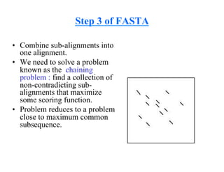
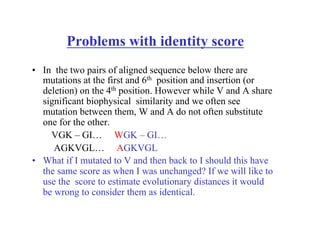
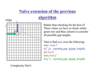
The document discusses pairwise sequence alignment and dynamic programming algorithms for computing optimal alignments. It covers:
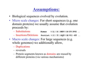
- Assumptions of sequence evolution including substitutions, insertions, deletions, duplications, and domain reuse.
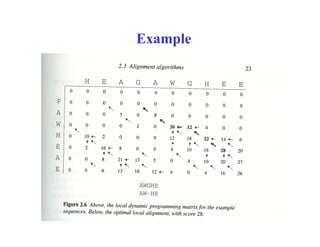
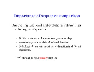
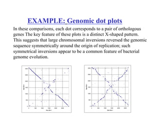
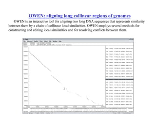
- Using sequence comparison to discover functional and evolutionary relationships by identifying similar sequences and orthologs with similar functions.
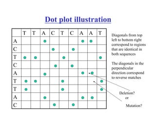
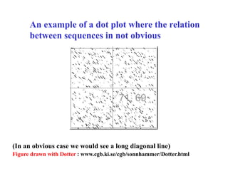
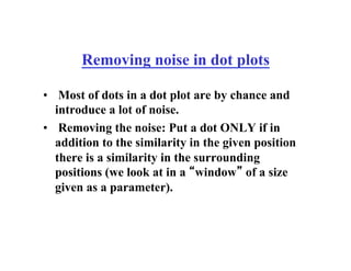
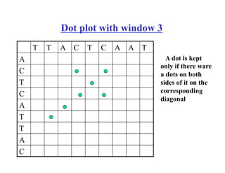
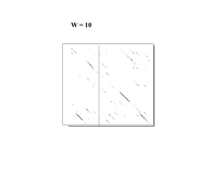
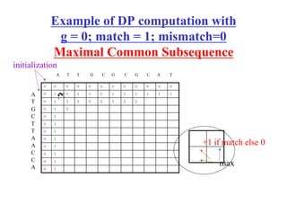
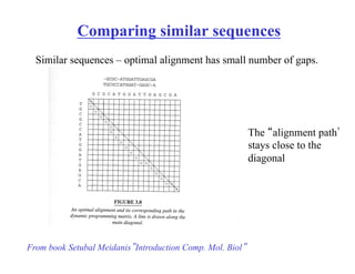
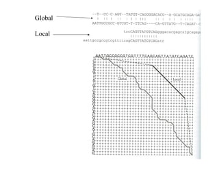
- The dot plot method for discovering sequence similarity by plotting sequences against each other in a matrix and identifying diagonals of matches.
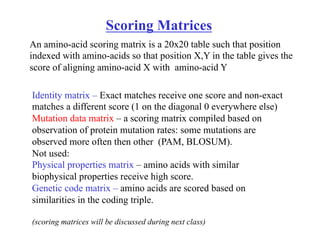
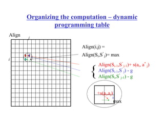
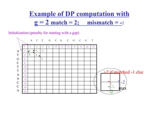
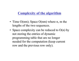
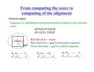
- Dynamic programming algorithms that compute the optimal alignment score in quadratic time and linear space by breaking the problem into overlapping subproblems.
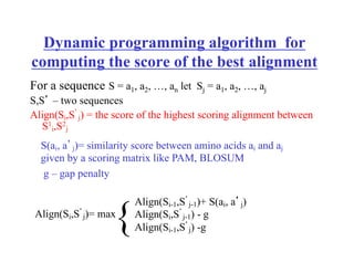
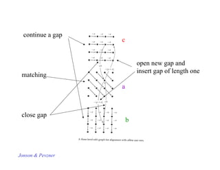
- Extensions of the basic algorithm to handle affine gap penalties by introducing three matrices to track alignments ending in matches, gaps


![The iterative algorithm
m = |S|; n = |S’|
for i " 0 to m do A[i,0]"- i * g
for j " 0 to n do A[0,j]" - j * g
for i " 1 to m do
for j " 1 to n
A[i,j]"max (
A[i-1,j] – g
A[i-1,j-1] + s(i,j)
A[i,j-1] – g
)
return(A[m,n])](https://image.slidesharecdn.com/pcblect02pairwiseallign1-221005062112-4ea8a175/85/PCB_Lect02_Pairwise_allign-1-pdf-23-320.jpg)
![Reducing space complexity in the
global alignment
Recall: Computing the score in linear space is easy.
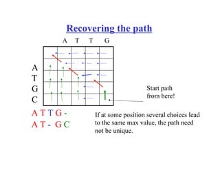
Leaving “trace” for finding optimal alignment is harder. Why?
OPT [ x
y ] be an optimal alignment between
sequence x and y
fix i, then there exist j such that OPT [ x
y ] can be obtained as
OPT [
x[1,…i-1]
y[1,…,j-1]]+
x[i]
y[j]
+ OPT
x[i+1,…m]
y[j+1,…,n]
[ ]
OPT
[
x[1,…i-1]
y[1,…,j] ]+
x[i]
-
+ OPT
x[i+1,…m]
y[j+1,…,n]
[ ]
OR
Let
Extra information not obligatory](https://image.slidesharecdn.com/pcblect02pairwiseallign1-221005062112-4ea8a175/85/PCB_Lect02_Pairwise_allign-1-pdf-27-320.jpg)
![Computing which of the two cases holds and for
what value of j:
1. Use dynamic programming for to compute the scores a[i,j] for
fixed i=n/2 and all j. O(nm/2)-time; linear space
2. Do the same for the suffixes. O(nm/2)-time; linear space
3. Find out which of the two cases from the previous case applies
and for which value of j.
4. Apply 1 & 2 recursively for the sequences to the left of (i,j)
and to the right of (i,j) (figure from previous slide)
Extra information – not obligatory](https://image.slidesharecdn.com/pcblect02pairwiseallign1-221005062112-4ea8a175/85/PCB_Lect02_Pairwise_allign-1-pdf-28-320.jpg)
![Ignoring initial and final gaps –
semiglobal comparison
Recall the initialization step for the dynamic programming table:
A[0,i] = ig; A[j,0]=jg – these are responsible for initial gaps.
set them to zero!
How to ignore final gaps?
CAGCA - CTTGGATTCTCGG
- - - CAGCGTGG - - - - - - - -
No penalties for
these gaps
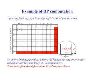
Take the largest value in the last row /column and trace-back form there](https://image.slidesharecdn.com/pcblect02pairwiseallign1-221005062112-4ea8a175/85/PCB_Lect02_Pairwise_allign-1-pdf-29-320.jpg)
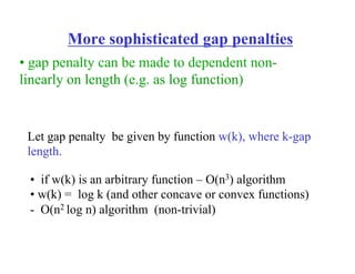
![General gap penalty
a[i,j]= max
a[i-1,j-1] + s(i,j)
max b[i,j-k] – w(k) for 0 <=k<=i
max b[i-k,j] – w(k) for 0 <=k<=j
{
w(k) any gap penalty function (not necessarily afine)
k = size of a gap.](https://image.slidesharecdn.com/pcblect02pairwiseallign1-221005062112-4ea8a175/85/PCB_Lect02_Pairwise_allign-1-pdf-33-320.jpg)
![O(n2) algorithm for afine gap penalty
We will have 3 dynamic programming tables:
s a[i,j] best possible alignment of Si and S’
j
s b[i,j] best possible alignment of Si and S’
j that ends with a gap in S
s c[i,j] best possible alignment of Si and S’
j that ends with a gap in S’
Let w(k) = h + gk
S1, S2 compared sequences
Text Pevzner’s book notation](https://image.slidesharecdn.com/pcblect02pairwiseallign1-221005062112-4ea8a175/85/PCB_Lect02_Pairwise_allign-1-pdf-34-320.jpg)
![Initialization
Assume that we charge for initial and terminal gaps
a[0,0] = 0;
a[i,0] = - infinity (i<>0);
a[0,j] = -infinity (j<>0)
b[i,0] = - infinity
b[0,j] = - (h+gj)
c[i,0] = - (h+gi)
c[0,j] = - infinity
-infinity is assigned where no alignment possible](https://image.slidesharecdn.com/pcblect02pairwiseallign1-221005062112-4ea8a175/85/PCB_Lect02_Pairwise_allign-1-pdf-37-320.jpg)
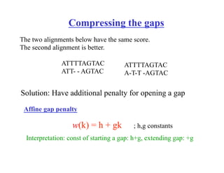
![Affine gap penalty function - cont
w(k) = h + gk ; h,g constants
Let a,b,c be as before. Now they can be completed as follows:
a[i,j]= max
a[i-1,j-1] + s(i,j)
b[i,j]
c[i,j]
{
b[i,j]= max
a[i,j-1] – (h+g) --- start a new gap in first seq
b[i,j-1] – g -- extend gap in second first by one
{
c[i,j]= max
a[i-1,j] – (h+g)
c[i-1,j] – g
{
Interpretation: const of starting a gap: h+g, extending gap: +g](https://image.slidesharecdn.com/pcblect02pairwiseallign1-221005062112-4ea8a175/85/PCB_Lect02_Pairwise_allign-1-pdf-38-320.jpg)
![k-band alignment
n = |S|= |S’|
for i " 0 to k do A[i,0]"- i * g
for j " 0 to k do A[0,j]" - j * g
for i " 1 to n do
for d " -k to k
j = i+d;
if inside_strip(i,j,k) then:
A[i,j]"max (
if inside_strip(i-1,j,k) then A[i-1,j] – g else -infinity
A[i-1,j-1] + s(i,j)
if inside_strip(i-1,j,k) then A[i,j-1] – g else -infinity
)
return(A[m,n])
Where insid _strip(i,j,k) is a test if cell A[i.j] is inside the strip that is if |i-j|<=k](https://image.slidesharecdn.com/pcblect02pairwiseallign1-221005062112-4ea8a175/85/PCB_Lect02_Pairwise_allign-1-pdf-43-320.jpg)
![Local alignment (Smith, Waterman)
So far we have been dealing with global alignment.
Local alignment – alignment between substrings.
Main idea: If alignment becomes to bad – drop it.
a[i,j]= max
a[i-1,j-1]+ s(ai, aj)
a[i-1,j +g
a[i,j-1]+ g
0
{
Set p and g so that alignment of random strings gives negative
score
Finding the alignment: find the highest scoring cell and trace it back](https://image.slidesharecdn.com/pcblect02pairwiseallign1-221005062112-4ea8a175/85/PCB_Lect02_Pairwise_allign-1-pdf-46-320.jpg)