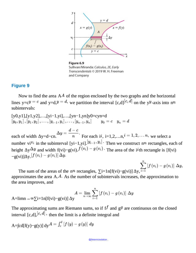
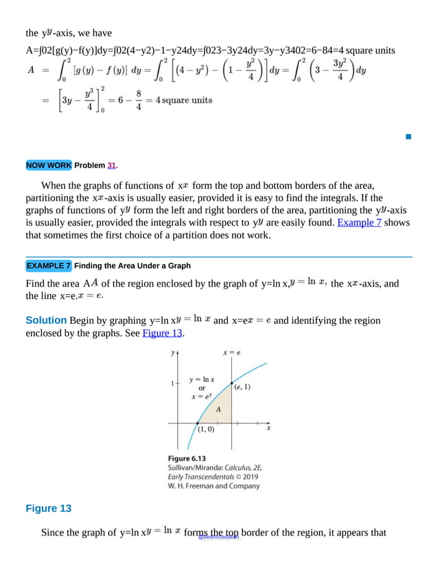
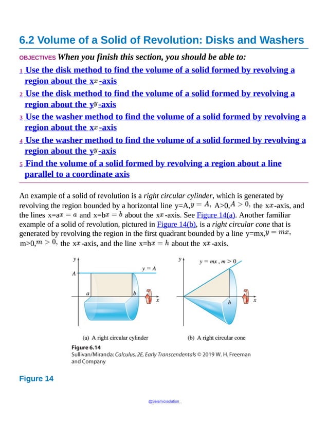
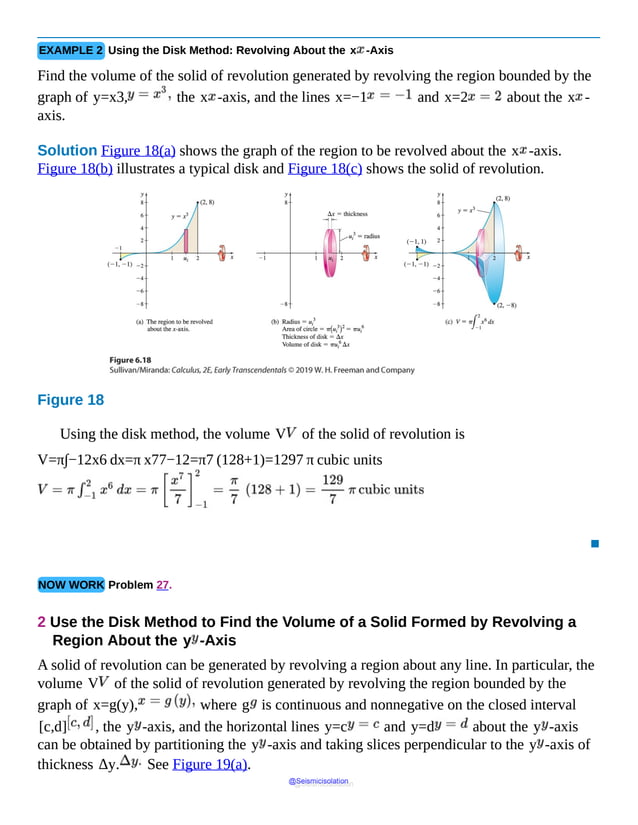
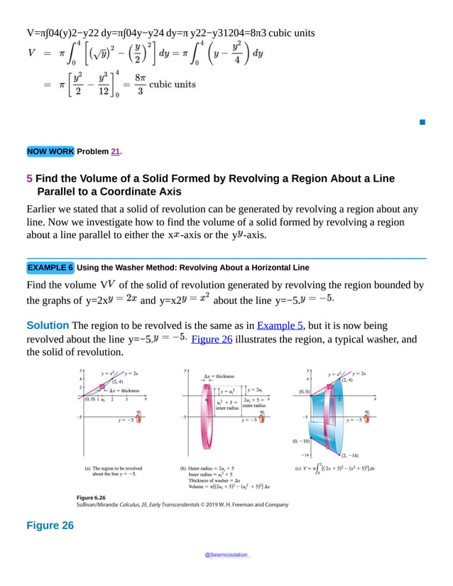
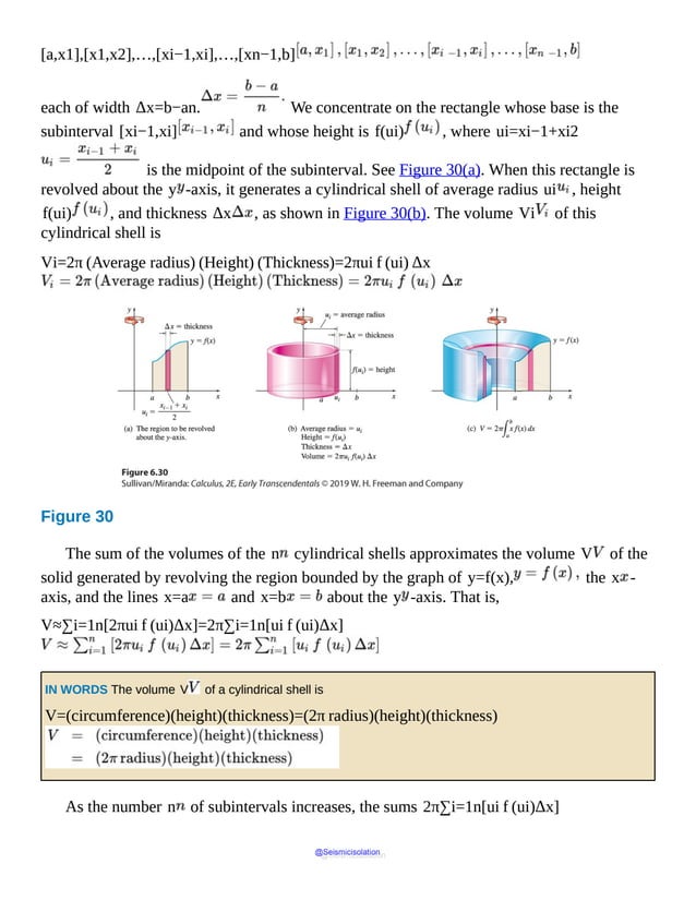
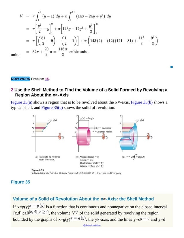
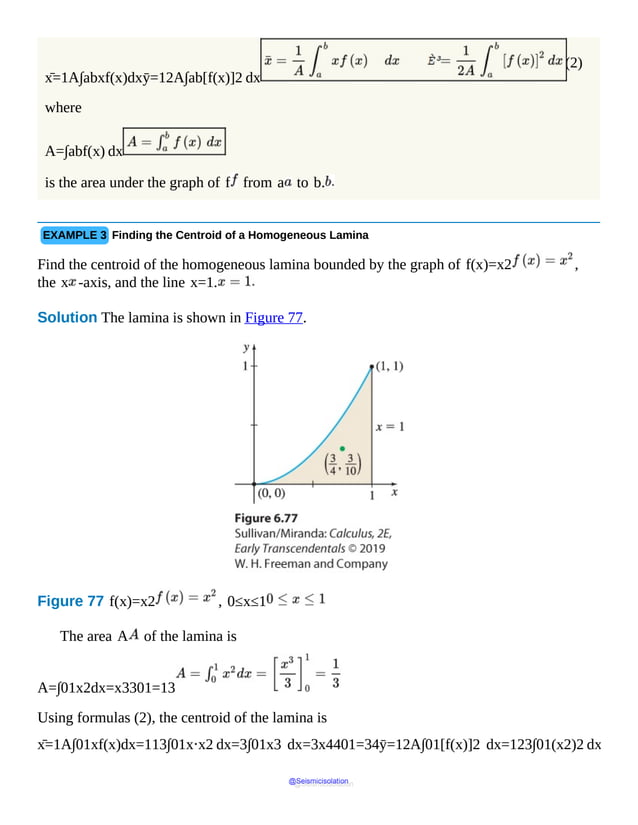
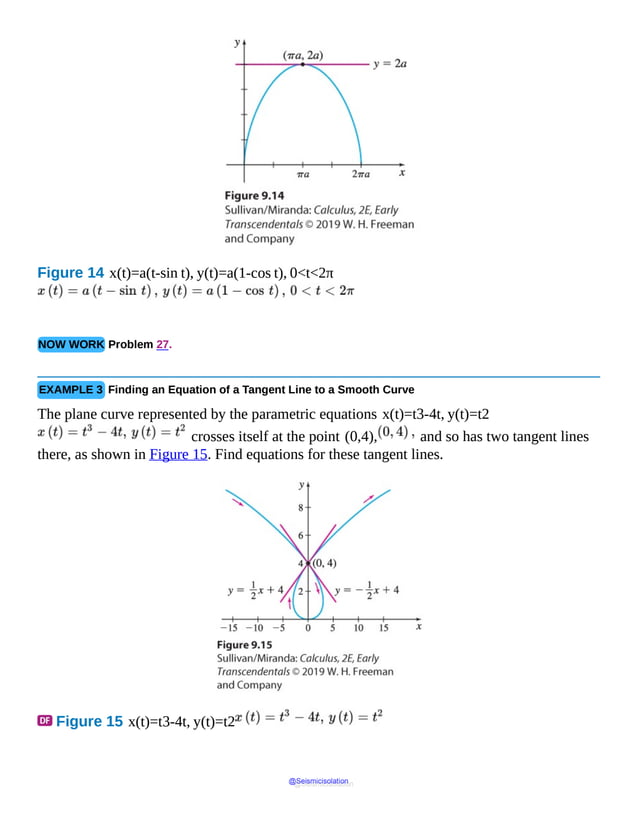
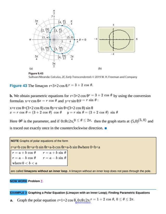
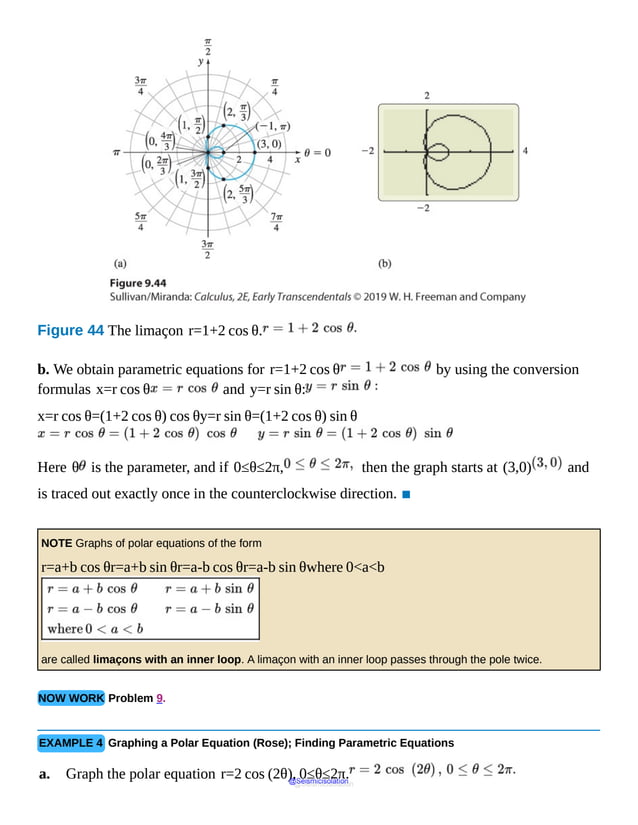
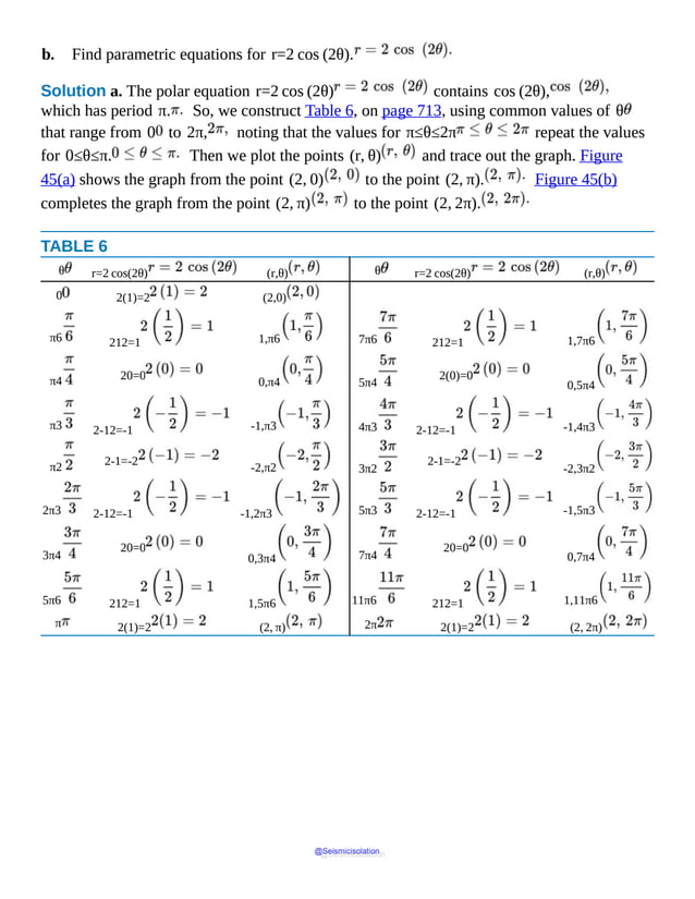
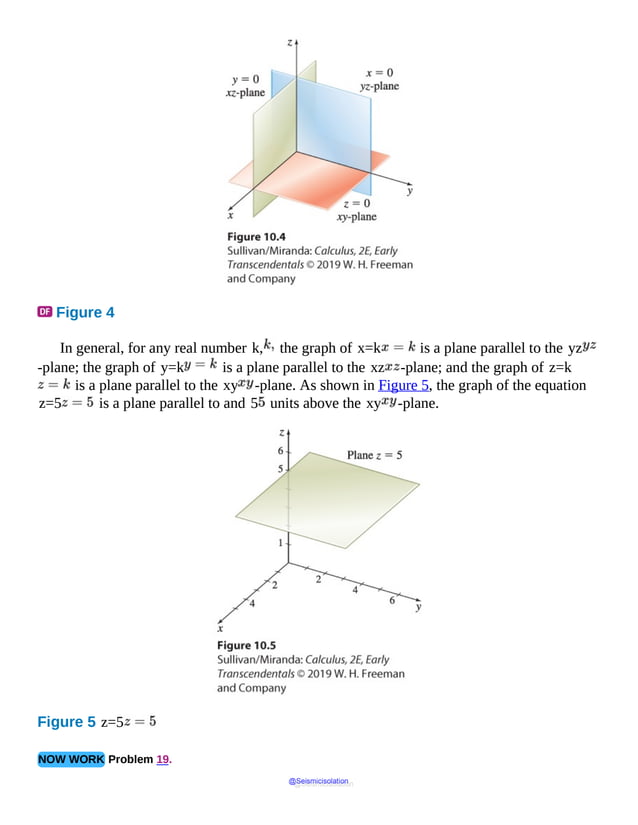
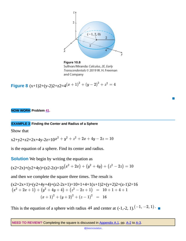
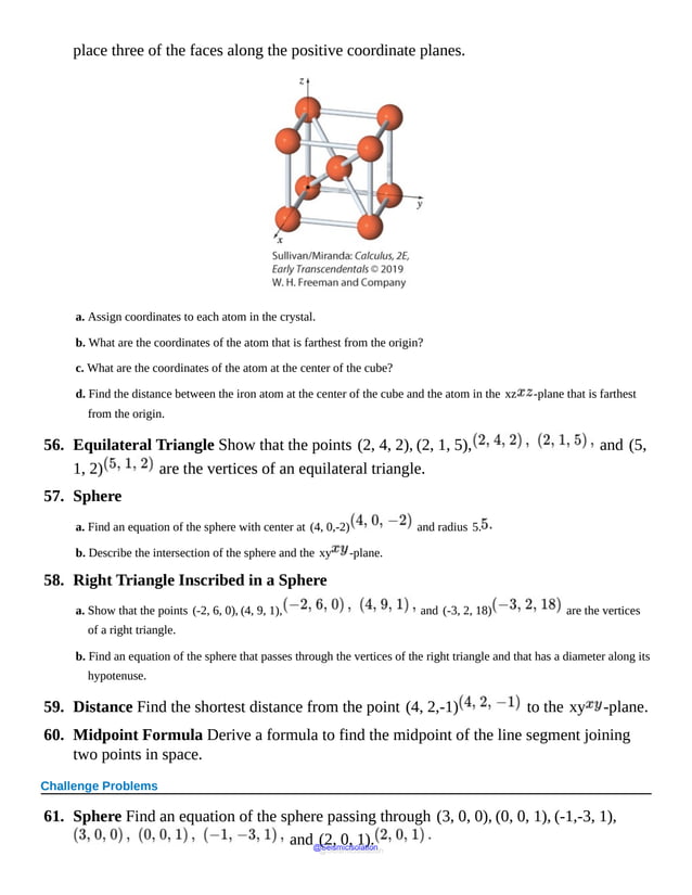
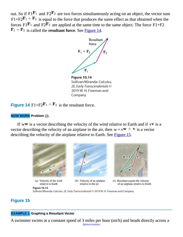
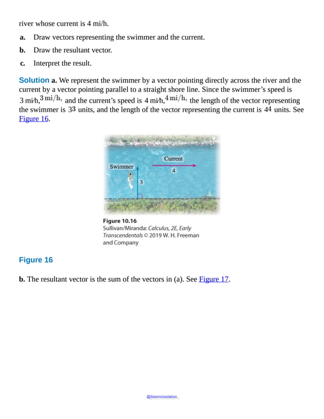
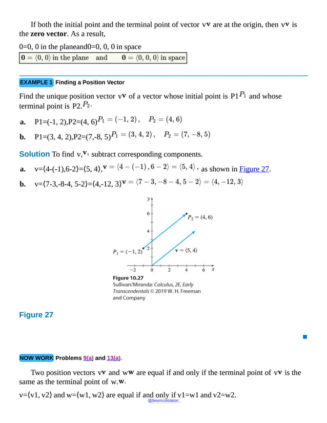
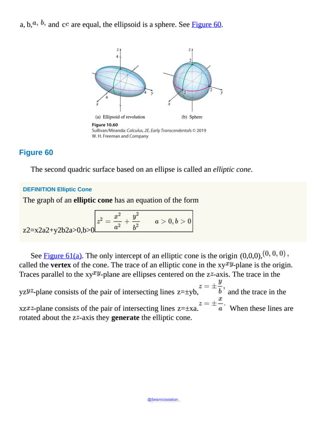
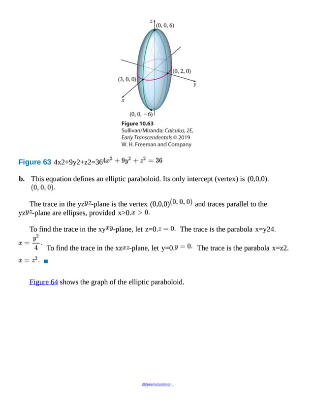
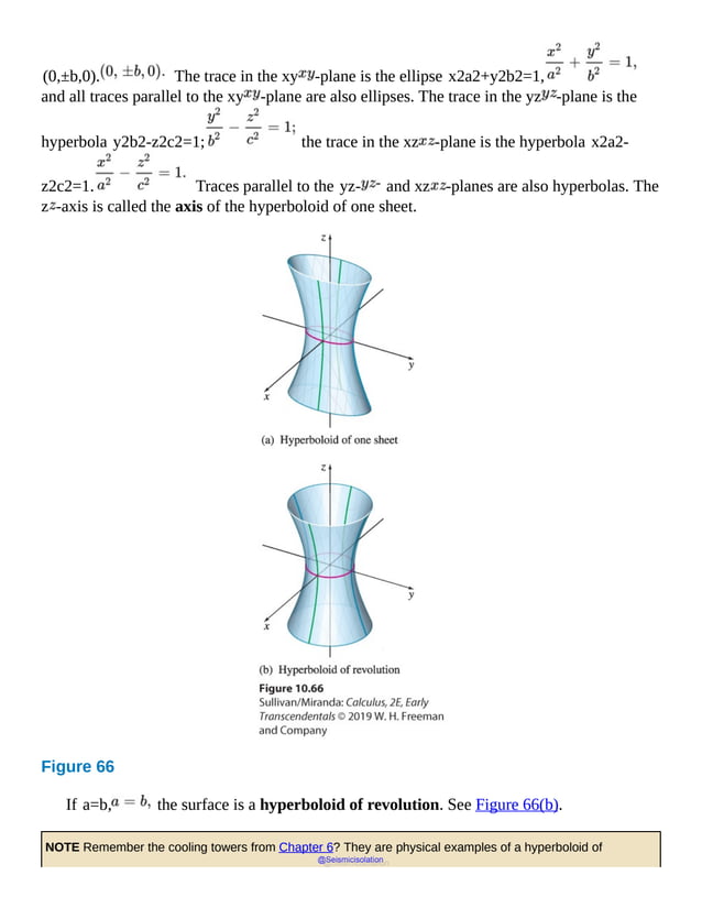
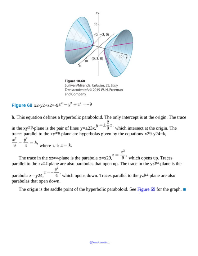
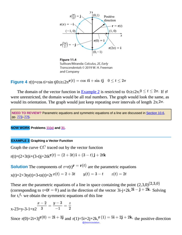
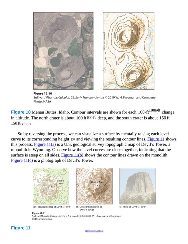
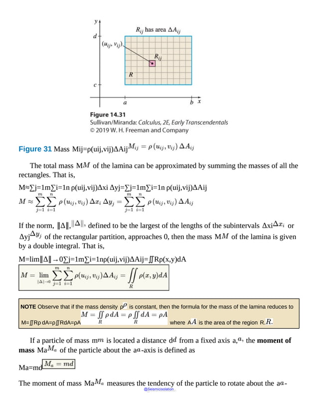
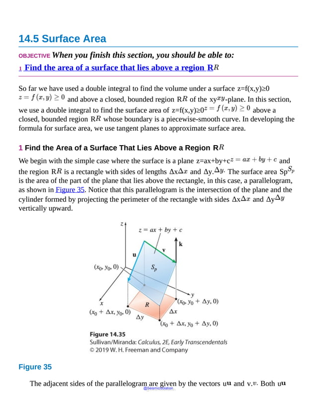
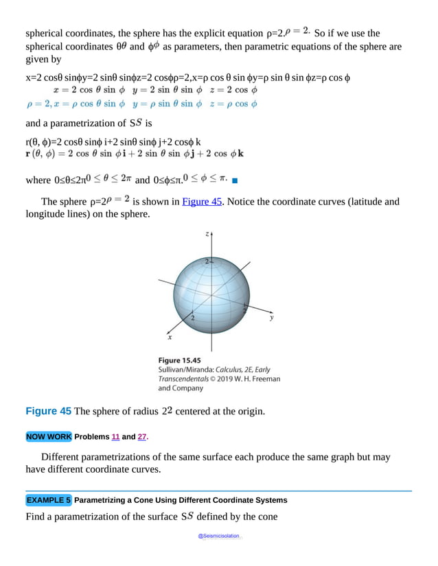
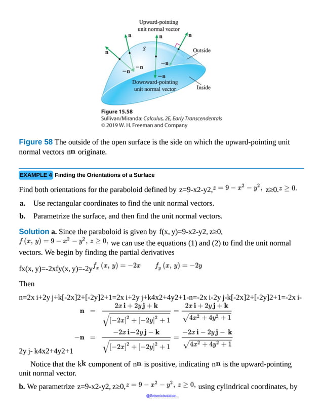
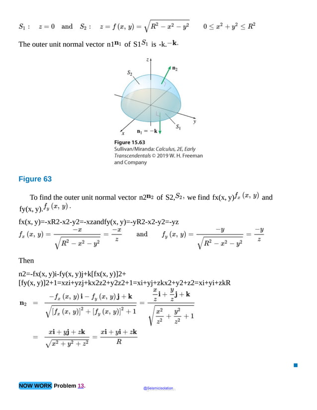
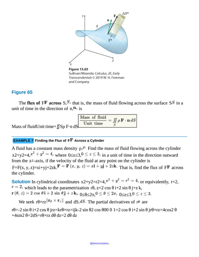
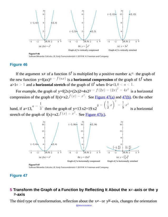
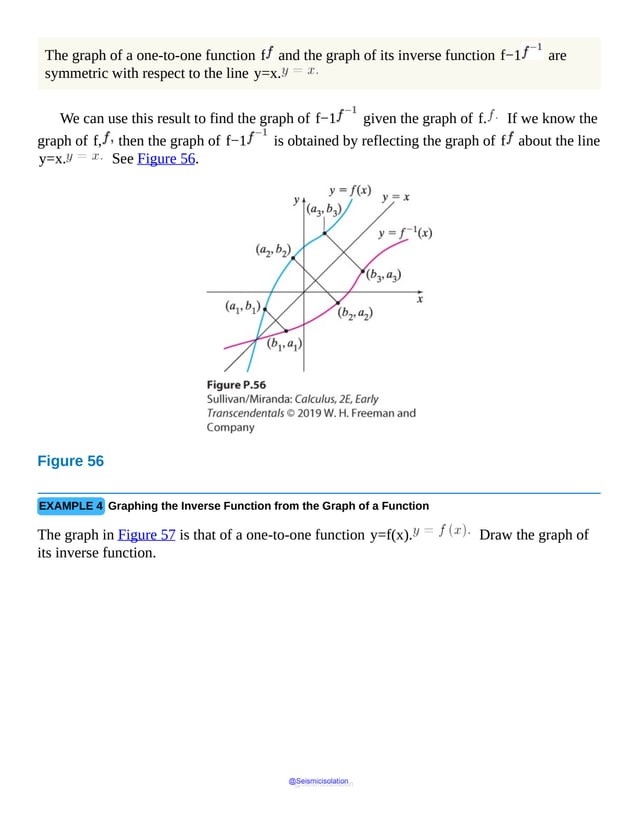
This document is the table of contents for Calculus, Early Transcendentals, Second Edition by Michael Sullivan. It lists 16 chapters that cover topics in calculus including limits, derivatives, integrals, vector calculus, and differential equations. The preface provides advice for students on how to effectively use the textbook to learn calculus, such as reading actively before class and using the examples and features to build understanding. The table of contents provides an overview of the scope and organization of content covered in the calculus textbook.

1. @Seismicisolation
@Seismicisolation

2. CALCULUS
EARLY TRANSCENDENTALS
SECOND EDITION
Michael Sullivan
Chicago State University
Kathleen Miranda
State University of New York, Old Westbury
@Seismicisolation
@Seismicisolation

3. Vice President, STEM: Daryl Fox
Program Director: Andrew Dunaway
Program Manager: Nikki Miller Dworsky
Development Editor: Andrew Sylvester
Associate Editor: Andy Newton
Editorial Assistant: Justin Jones
Senior Marketing Manager: Nancy Bradshaw
Marketing Assistant: Savannah DiMarco
Executive Media Editor: Catriona Kaplan
Assistant Media Editor: Doug Newman
Director of Digital Production: Keri deManigold
Senior Media Project Manager: Alison Lorber
Photo Editor: Christine Buese
Photo Research: Donna Ranieri
Director of Content Management Enhancement: Tracey Kuehn
Managing Editor: Lisa Kinne
Director of Design, Content Management: Diana Blume
Text Design: Diana Blume
Senior Content Project Manager: Edgar Doolan
Senior Workflow Manager: Paul Rohloff
Illustration Coordinator: Janice Donnola
Illustrations: Network Graphics
Composition: Lumina Datamatics Ltd.
ISBN-13: 978-1-319-24848-2 (epub)
© 2019, 2014 by W. H. Freeman and Company
All rights reserved.
1 2 3 4 5 6 23 22 21 20 19
W. H. Freeman and Company
One New York Plaza
Suite 4500
New York, NY 10004-1562
www.macmillanlearning.com
@Seismicisolation
@Seismicisolation

4. What Is Calculus?
Calculus is a part of mathematics that evolved much later than other subjects. Algebra,
geometry, and trigonometry were developed in ancient times, but calculus as we know it did
not appear until the seventeenth century.
The first evidence of calculus has its roots in ancient mathematics. For example, In his
book A History of π, Petr Beckmann explains that Greek mathematician Archimedes (287–
212 BCE) “took the step from the concept of ‘equal to’ to the concept of ‘arbitrarily close to’
or ‘as closely as desired’…and reached the threshold of the differential calculus, just as his
method of squaring the parabola reached the threshold of the integral calculus.”* But it was
not until Sir Isaac Newton and Gottfried Wilhelm Leibniz, each working independently,
expanded, organized, and applied these early ideas, that the subject we now know as calculus
was born.
Although we attribute the birth of calculus to Newton and Leibniz, many other
mathematicians, particularly those in the eighteenth and nineteenth centuries, contributed
greatly to the body and rigor of calculus. You will encounter many of their names and
contributions as you pursue your study of calculus.
But what is calculus?
The simple answer is: calculus models change. Since the world and most things in it are
constantly changing, mathematics that explains change becomes immensely useful.
Calculus has two major branches, differential calculus and integral calculus. Let’s take a
peek at what calculus is by looking at two problems that prompted the development of
calculus.
The Tangent Problem—The Basis of Differential Calculus
Suppose we want to find the slope of the line tangent to the graph of a function at some point
P=(x1, y1). See Figure 1(a). Since the tangent line necessarily contains the
point P, it remains only to find the slope to identify the tangent line. Suppose we repeatedly
zoom in on the graph of the function at the point P. See Figure 1(b). If we can zoom in close
enough, then the graph of the function will look approximately linear, and we can choose a
point Q, on the graph of the function different from the point P, and use the formula for
slope.
@Seismicisolation
@Seismicisolation

5. Figure 1
Repeatedly zooming in on the point P is equivalent to choosing a point Q closer and closer to
the point P. Notice that as we zoom in on P, the line connecting the points P and Q, called a
secant line, begins to look more and more like the tangent line to the graph of the function at
the point P. If the point Q can be made as close as we please to the point P, without equaling
the point P, then the slope of the tangent line mtan can be found. This formulation leads
to differential calculus, the study of the derivative of a function.
The derivative gives us information about how a function changes at a given instant and can
be used to solve problems involving velocity and acceleration; marginal cost and profit; and
the rate of change of a chemical reaction. Derivatives are the subjects of Chapters 2 through
4.
The Area Problem—The Basis of Integral Calculus
If we want to find the area of a rectangle or the area of a circle, formulas are available. (See
Figure 2.) But what if the figure is curvy, but not circular as in Figure 3? How do we find this
area?
Figure 2
@Seismicisolation
@Seismicisolation

6. Figure 3
Calculus provides a way. Look at Figure 4(a). It shows the graph of y=x2 from
x=0 to x=1. Suppose we want to find the area of the shaded region.
Figure 4
By subdividing the x-axis from 0 to 1 into small segments and drawing a rectangle of
height x2 above each segment, as in Figure 4(b), we can find the area of each rectangle
and add them together. This sum approximates the shaded area in Figure 4(a). The smaller
we make the segments of the x-axis and the more rectangles we draw, the better the
approximation becomes. See Figure 4(c). This formulation leads to integral calculus, and the
study of the integral of a function.
Two Problems—One Subject?
At first differential calculus (the tangent problem) and integral calculus (the area problem)
@Seismicisolation
@Seismicisolation

7. appear to be different, so why call both of them calculus? The Fundamental Theorem of
Calculus establishes that the derivative and the integral are related. In fact, one of Newton’s
teachers, Isaac Barrow, recognized that the tangent problem and the area problem are closely
related, and that derivatives and integrals are inverses of each other. Both Newton and
Leibniz formalized this relationship between derivatives and integrals in the Fundamental
Theorem of Calculus.
*Beckmann, P. (1976). A History of π (3rd. ed., p. 64). New York: St. Martin’s Press.
@Seismicisolation
@Seismicisolation

8. Contents | Calculus, Early Transcendentals,
Second Edition
Preface
Applications Index
@Seismicisolation
@Seismicisolation

9. P Preparing for Calculus
P.1 Functions and Their Graphs
P.2 Library of Functions; Mathematical Modeling
P.3 Operations on Functions; Graphing Techniques
P.4 Inverse Functions
P.5 Exponential and Logarithmic Functions
P.6 Trigonometric Functions
P.7 Inverse Trigonometric Functions
P.8 Sequences; Summation Notation; the Binomial Theorem
1 Limits and Continuity
1.1 Limits of Functions Using Numerical and Graphical Techniques
1.2 Limits of Functions Using Properties of Limits
1.3 Continuity
1.4 Limits and Continuity of Trigonometric, Exponential, and Logarithmic Functions
1.5 Infinite Limits; Limits at Infinity; Asymptotes
1.6 The ε−δ Definition of a Limit
Chapter Review
Chapter Project: Pollution in Clear Lake
2 The Derivative
2.1 Rates of Change and the Derivative
2.2 The Derivative as a Function
2.3 The Derivative of a Polynomial Function; The Derivative of y=ex
2.4 Differentiating the Product and the Quotient of Two Functions; Higher-Order Derivatives
2.5 The Derivative of the Trigonometric Functions
Chapter Review
Chapter Project: The Lunar Module
3 More About Derivatives
3.1 The Chain Rule
3.2 Implicit Differentiation
3.3 Derivatives of the Inverse Trigonometric Functions
3.4 Derivatives of Logarithmic Functions
3.5 Differentials; Linear Approximations; Newton’s Method
3.6 Hyperbolic Functions
Chapter Review
Chapter Project: World Population
4 Applications of the Derivative
4.1 Related Rates
@Seismicisolation
@Seismicisolation

10. 4.2 Maximum and Minimum Values; Critical Numbers
4.3 The Mean Value Theorem
4.4 Local Extrema and Concavity
4.5 Indeterminate Forms and L’Hôpital’s Rule
4.6 Using Calculus to Graph Functions
4.7 Optimization
4.8 Antiderivatives; Differential Equations
Chapter Review
Chapter Project: The U.S. Economy
5 The Integral
5.1 Area
5.2 The Definite Integral
5.3 The Fundamental Theorem of Calculus
5.4 Properties of the Definite Integral
5.5 The Indefinite Integral; Method of Substitution
5.6 Separable First-Order Differential Equations; Uninhibited and Inhibited Growth and Decay Models
Chapter Review
Chapter Project: Managing the Klamath River
6 Applications of the Integral
6.1 Area Between Graphs
6.2 Volume of a Solid of Revolution: Disks and Washers
6.3 Volume of a Solid of Revolution: Cylindrical Shells
6.4 Volume of a Solid: Slicing
6.5 Arc Length; Surface Area of a Solid of Revolution
6.6 Work
6.7 Hydrostatic Pressure and Force
6.8 Center of Mass; Centroid; The Pappus Theorem
Chapter Review
Chapter Project: Determining the Amount of Concrete Needed for a Cooling Tower
7 Techniques of Integration
7.1 Integration by Parts
7.2 Integrals Containing Trigonometric Functions
7.3 Integration Using Trigonometric Substitution: Integrands Containing a2−x2,x2+a2, or x2−a2, a>0
7.4 Integrands Containing ax2+bx+c, a≠0
7.5 Integration of Rational Functions Using Partial Fractions; the Logistic Model
7.6 Approximating Integrals: The Trapezoidal Rule, the Midpoint Rule, Simpson’s Rule
7.7 Improper Integrals
7.8 Integration Using Tables and Computer Algebra Systems
@Seismicisolation
@Seismicisolation

11. 7.9 Mixed Practice
Chapter Review
Chapter Project: The Birds of Rügen Island
8 Infinite Series
8.1 Sequences
8.2 Infinite Series
8.3 Properties of Series; Series with Positive Terms; the Integral Test
8.4 Comparison Tests
8.5 Alternating Series; Absolute Convergence
8.6 Ratio Test; Root Test
8.7 Summary of Tests
8.8 Power Series
8.9 Taylor Series; Maclaurin Series
8.10 Approximations Using Taylor/Maclaurin Expansions
Chapter Review
Chapter Project: How Calculators Calculate
9 Parametric Equations; Polar Equations
9.1 Parametric Equations
9.2 Tangent Lines
9.3 Arc Length; Surface Area of a Solid of Revolution
9.4 Polar Coordinates
9.5 Polar Equations; Parametric Equations of Polar Equations; Arc Length of Polar Equations
9.6 Area in Polar Coordinates
9.7 The Polar Equation of a Conic
Chapter Review
Chapter Project: Polar Graphs and Microphones
10 Vectors; Lines, Planes, and Quadric Surfaces in Space
10.1 Rectangular Coordinates in Space
10.2 Introduction to Vectors
10.3 Vectors in the Plane and in Space
10.4 The Dot Product
10.5 The Cross Product
10.6 Equations of Lines and Planes in Space
10.7 Quadric Surfaces
Chapter Review
Chapter Project: The Hall Effect
11 Vector Functions
11.1 Vector Functions and Their Derivatives
11.2 Unit Tangent and Principal Unit Normal Vectors; Arc Length
@Seismicisolation
@Seismicisolation

12. 11.3 Arc Length as Parameter; Curvature
11.4 Motion Along a Curve
11.5 Integrals of Vector Functions; Projectile Motion
11.6 Application: Kepler’s Laws of Planetary Motion
Chapter Review
Chapter Project: How to Design a Safe Road
12 Functions of Several Variables
12.1 Functions of Two or More Variables and Their Graphs
12.2 Limits and Continuity
12.3 Partial Derivatives
12.4 Differentiability and the Differential
12.5 Chain Rules
Chapter Review
Chapter Project: Searching for Exoplanets
13 Directional Derivatives, Gradients, and Extrema
13.1 Directional Derivatives; Gradients
13.2 Tangent Planes
13.3 Extrema of Functions of Two Variables
13.4 Lagrange Multipliers
Chapter Review
Chapter Project: Measuring Ice Thickness on Crystal Lake
14 Multiple Integrals
14.1 The Double Integral over a Rectangular Region
14.2 The Double Integral over Nonrectangular Regions
14.3 Double Integrals Using Polar Coordinates
14.4 Center of Mass; Moment of Inertia
14.5 Surface Area
14.6 The Triple Integral
14.7 Triple Integrals Using Cylindrical Coordinates
14.8 Triple Integrals Using Spherical Coordinates
14.9 Change of Variables Using Jacobians
Chapter Review
Chapter Project: The Mass of Stars
15 Vector Calculus
15.1 Vector Fields
15.2 Line Integrals of Scalar Functions
15.3 Line Integrals of Vector Fields; Work
15.4 Fundamental Theorem of Line Integrals
15.5 Green’s Theorem
@Seismicisolation
@Seismicisolation

13. 15.6 Parametric Surfaces
15.7 Surface and Flux Integrals
15.8 The Divergence Theorem
15.9 Stokes’ Theorem
Chapter Review
Chapter Project: Modeling a Tornado
16 Differential Equations
16.1 Classification of Ordinary Differential Equations
16.2 Separable and Homogeneous First-Order Differential Equations; Slope Fields; Euler’s Method
16.3 Exact Differential Equations
16.4 First-Order Linear Differential Equations; Bernoulli Differential Equations
16.5 Power Series Methods
Chapter Review
Chapter Project: The Melting Arctic Ice Cap
APPENDIX A Precalculus Used in Calculus
A.1 Algebra Used in Calculus
A.2 Geometry Used in Calculus
A.3 Analytic Geometry Used in Calculus
A.4 Trigonometry Used in Calculus
APPENDIX B Theorems and Proofs
B.1 Limit Theorems and Proofs
B.2 Theorems and Proofs Involving Inverse Functions
B.3 Derivative Theorems and Proofs
B.4 Integral Theorems and Proofs
B.5 A Bounded Monotonic Sequence Converges
B.6 Taylor’s Formula with Remainder
APPENDIX C Technology Used in Calculus
C.1 Graphing Calculators
C.2 Computer Algebra Systems (CAS)
Answers
Index
@Seismicisolation
@Seismicisolation

14. Preface
To the Student
As you begin your calculus course, you may feel anxious about the large number of
theorems, definitions, problems, and pages that you see in the book. Don’t worry, your
concerns are normal. As educators we understand the challenges you face in this course, and
as authors we have crafted a text that gives you the tools to meet them. If you pay attention in
class, keep up with your homework, and read and study what is in this book, you will build
the knowledge and skills you need to be successful. Here are some ways that you can use the
book to your benefit.
Read actively. When you are busy, it is tempting to skip reading and go right to the
problems. Don’t! This book has examples with clear explanations to help you learn how to
logically solve mathematics problems. Reading the book actively, with a pencil in hand,
and doing the worked examples along with us will help you develop a clearer
understanding than you will get from simple memorization.
Read before class, not after. If you do, the classroom lecture will sound familiar, and you
can ask questions about material you don’t understand. You’ll be amazed at how much
more you get out of class if you read first.
Use the examples. Mastering calculus requires a deep understanding of the concepts.
Read and work the examples, and do the suggested NOW WORK Problems listed after
them. Also do all the problems your instructor assigns. Be sure to seek help as soon as you
feel you need it.
Use the book’s features. In the classroom, we use many methods to communicate. These
methods are reflected in various features that we have created for this book. These
features, described on the following pages, are designed to make it easier for you to
understand, review, and practice. Taking advantage of the features will help you to master
calculus.
Engage with the applications. Students come to this course with a wide variety of
educational goals. You may be majoring in life sciences or social sciences, business or
economics, engineering or mathematics. This book has many applied exercises—some
written by students like you—related to courses in a wide variety of majors.
Please do not hesitate to contact us with any questions, sug​gestions, or comments that might
improve this text. We look forward to hearing from you, and we hope that you enjoy learning
calculus and do well—not only in calculus but in all your studies.
Best Wishes,
@Seismicisolation
@Seismicisolation

15. Michael Sullivan and Kathleen Miranda
To the Instructor
The challenges facing calculus instructors are daunting. Diversity among students, both in
their mathematical preparedness for learning calculus and in their ultimate educational and
career goals, is vast and growing. Increased emphasis by universities and administrators on
structured assessment and its related data analytics puts additional demands on instructors.
There is not enough classroom time to teach every topic in the syllabus, to answer every
student’s questions, or to delve into the rich examples and applications that showcase the
beauty and utility of calculus. As mathematics instructors, we share these frustrations. As
authors, our goal is to craft a calculus textbook that supports your teaching philosophy,
promotes student understanding, and identifies measurable learning outcomes.
Calculus, Early Transcendentals, Second Edition, is a mathematically precise calculus
book that embraces proven pedagogical strategies to increase both student and instructor
success.
The language of the text is simple, clear, and precise. Definitions and theorems are
carefully stated, and titled when appropriate. Numbering of definitions, equations, and
theorems is kept to a minimum.
The mathematics is rigorous. Proofs of theorems are presented throughout the text in one
of three ways: (1) following the statement of a theorem; (2) preceding a theorem followed
by “We have proved the following theorem”; or (3) in Appendix B, if the proof is more
involved. (When the proof of a theorem is beyond the scope of this book, we note that it
may be found in advanced calculus or numerical analysis texts.)
The text is adaptable to your class and your teaching style. Proofs can be included or
omitted and exercises are paired, grouped, and graduated from easy to difficult. By
dividing exercises into Skill Building, Applications and Extensions, and Challenge
Problems, we make it easier for you to tailor assignments to the specific needs of your
students based on their ability and preparedness.
The structural pedagogical features, described on the pages that follow, can be used to
design an assessment tool for your students. Learning objectives are listed at the start of
each section; the structure of the solved examples and/or the proofs can be used to write
rubrics for evaluation; and assessment questions can be drawn from the Now Work
Problems, end of section exercises, and chapter review problems. Additional media and
supplement resources available to you and your students are described on page xiii.
Let us know what you think of the text and do not hesitate to contact us with any suggestions
or comments that might improve it. We look forward to hearing from you.
@Seismicisolation
@Seismicisolation

16. Best Wishes,
Michael Sullivan and Kathleen Miranda
Pedagogical Features Promote Student Success
Just In Time Review Throughout the text there are margin notes labeled NEED TO
REVIEW? followed by a topic and page references. These references point to a previous
presentation of a concept related to the discussion at hand.
RECALL margin notes provide a quick refresher of key results that are being used in
theorems, definitions, and examples.
IN WORDS These notes translate complex formulas, theorems, proofs, rules, and definitions
using plain language that provide students with an alternate way to learn the concepts.
CAUTIONS and NOTES provide supporting details or warnings about common pitfalls.
ORIGINS give biographical information or historical details about key figures and
discoveries in the development of calculus.
@Seismicisolation
@Seismicisolation

17. Effective Use of Color The text contains an abundance of graphs and illustrations that
carefully utilize color to make concepts easier to visualize.
Dynamic Figures The text includes many pieces of art that students can interact with
through the online e-Book. These dynamic figures, indicated by the icon next to the
figure label, illustrate select principles of calculus, including limits, rates of change, solids of
revolution, convergence, and divergence.
@Seismicisolation
@Seismicisolation

18. Learning Objectives Each section begins with a set of Objectives that serve as a broad
outline of the section. The objectives help students study effectively by focusing attention on
the concepts being covered. Each learning objective is supported by appropriate definitions,
theorems, and proofs. One or more carefully chosen examples enhance the learning
objective, and where appropriate, an application example is also included. Learning
objectives help instructors prepare a syllabus that includes the important topics of calculus,
and concentrate instruction on mastery of these topics.
Examples with Detailed and Annotated Solutions Examples are named according to their
purpose. The text includes hundreds of examples with detailed step-by-step solutions.
Additional annotations provide the formula used, or the reasoning needed, to perform a
particular step of the solution. Where procedural steps for solving a type of problem are
given in the text, these steps are followed in the solved examples. Often a figure or a graph is
included to complement the solution.
@Seismicisolation
@Seismicisolation

19. Chapter Projects The case studies that open each chapter demonstrate how major concepts
apply to recognizable and often contemporary situations in biology, environmental studies,
astronomy, engineering, technology, and other fields. At the end of the chapter, there is an
extended project with questions that guide students through a solution to the situation.
Immediate Reinforcement of Skills Following most examples there is the statement, NOW
WORK. This callout directs students to a related exercise from the section’s problem set.
Doing a related problem immediately after working through a solved example encourages
@Seismicisolation
@Seismicisolation

20. active learning, enhances understanding, and strengthens a student’s ability to use the
objective. This practice also serves as a confidence-builder for students.
The Exercises are Divided into Four Categories
Concepts and Vocabulary provide a selection of quick fill-in-the-blank, multiple choice,
and true/false questions. These problems assess a student’s comprehension of the main points
of the section.
Skill Building problems are grouped into subsets, usually corresponding to the objectives of
the section. Problem numbers in red are the NOW WORK problems that are correlated to
the solved examples. The skill building problems are paired by odd/even and usually
progress from easy to difficult.
@Seismicisolation
@Seismicisolation

21. Applications and Extensions consist of applied problems, questions that require proof, and
problems that extend the concepts of the section. (See the Applications Index for a full list of
the applied examples and problems in the text.)
Challenge Problems provide more difficult extensions of the section’s material. They are
often combined with concepts learned in previous chapters. Challenge problems are intended
to be thought-provoking and require some ingenuity to solve—they are an excellent addition
@Seismicisolation
@Seismicisolation

22. to assignments for exceptionally strong students or for use in group work.
The Chapter Review is in Three Parts
Things to Know is a detailed list of important definitions, formulas, and theorems contained
in the chapter, and page references to where they can be found.
Objectives Table is a section-by-section list of each learning objective of the chapter (with
page references), as well as references to the solved examples and review problems related to
that learning objective.
@Seismicisolation
@Seismicisolation

23. Review Problems provide exercises related to the key concepts of the chapter and are
matched to the learning objectives of each section of the chapter.
New to the Second Edition
The Second Edition of Calculus, Early Transcendentals, is the culmination of more than 100
reviews of the first edition, more than 20 focus groups, and 4 years of work. Contributions
came from a variety of sources: students who studied from the first edition, as well as
professors at community colleges, 4-year universities, and research universities, some of
whom taught from the first edition and some of whom did not. We also commissioned a team
of reputable mathematicians to review every aspect of the revised presentation. Using this
invaluable input, as well as insights from our own experiences teaching calculus, we have
revised and modified as needed, while preserving the writing style and presentation that
students using the first edition praise.
We acknowledge the crucial importance of clarity and rigor, particularly considering the
investment an instructor makes when adopting a calculus textbook. In preparing for this
revision, we analyzed every component of the text: content, organization, examples,
exercises, rigor, mathematical accuracy, depth and breadth of coverage, accessibility, and
readability. Reviewers suggested how and where to revise, cut, deepen, or expand the
@Seismicisolation
@Seismicisolation

24. coverage. Many offered suggestions for new exercises or nuances to enhance a student’s
learning experience. Wherever new Objectives or Examples were added, corresponding
problems in the exercise sets were also added.
A brief description of the major changes to the content and organization in the second
edition is provided below. It is by no means comprehensive and does not reflect the more
subtle, but no less important, changes we made in our quest to increase clarity and deepen
conceptual understanding.
Chapter P Preparing for Calculus
Sequences; Summation Notation; the Binomial Theorem has been moved from Appendix
A to Chapter P, and now includes a full exercise set.
Chapter 2 The Derivative
Section 2.2 includes NEW EXAMPLES on obtaining information about a function from
the graph of its derivative function and determining whether a (piecewise-defined)
function has a derivative at a number.
Chapter 3 More About Derivatives
Implicit Differentiation and Derivatives of Inverse Trigo​nometric Functions are now
treated in separate sections.
The discussion of Taylor Polynomials (previously Section 3.5) is now in Chapter 8
(Infinite Series).
Chapter 4 Applications of the Derivative
Section 4.3 includes a NEW EXAMPLE on obtaining information about the graph of a
function from the graph of its derivative.
Section 4.4 includes NEW EXAMPLES on obtaining information about the graph of a
function f from the graphs of f′ and f″.
Chapter 5 The Integral
Section 5.2 The Definite Integral has been rewritten and expanded to accommodate the
following objectives:
Form Riemann sums
Define a definite integral as a limit of Riemann sums
Approximate a definite integral using Riemann sums
Know conditions that guarantee a definite integral exists
Find a definite integral using the limit of Riemann sums
Form Riemann sums from a table @Seismicisolation
@Seismicisolation

25. To improve conceptual understanding, three new interpretations of the definite integral
have been included:
Section 5.3: Objective 3: Interpret the integral as a rate of change, accompanied by two
new examples, and Objective 4: Interpret the integral as an accumulation function,
accompanied by a new example.
Section 5.4: Objective 4: Interpreting integrals involving rectilinear motion.
Section 5.5: The Indefinite Integral and Substitution are now treated in one section.
Section 5.6 now covers separable first-order differential equations and growth and decay
models (both uninhibited and inhibited).
Chapter 6 Applications of the Integral
Section 6.5: NEW Objective 3: Find the surface area of a solid of revolution.
Chapter 7 Techniques of Integration
Section 7.1: NEW Objective 2: Find a definite integral using integration by parts.
Section 7.2: NEW Summary tables are now included.
Section 7.5: NEW Objective 5: Solve the logistic differen​tial equation.
Section 7.6: NEW Objective 2: Approximate an integral using the Midpoint Rule.
NEW Section 7.9: Mixed Practice provides exercises that “mix up” all the integrals.
Chapter 8 Infinite Series
Section 8.3: NEW Objective 5: Approximating the sum of a convergent series.
Section 8.4 now includes an expanded form of the Limit Comparison Test.
Section 8.10: NEW Objective 1: Approximate a function and its graph using a Taylor
Polynomial.
Chapter 9 Parametric Equations; Polar Equations
Arc length, formerly in Section 9.2, now appears in Section 9.3.
Chapter 11 Vector Functions
Section 11.5 has been expanded to include more examples of both indefinite and definite
integrals of vector functions.
Chapter 12 Functions of Several Variables
Section 12.3 now includes an example that uses the definition to find the partial
@Seismicisolation
@Seismicisolation

26. derivatives of a function on two variables, and an example that uses the Chain Rule to find
partial derivatives has been added.
Chapter 13 Directional Derivatives, Gradients, and Extrema
Section 13.1 has an increased emphasis on the geometric interpretation of the gradient.
Section 13.2: NEW Objective 3: Find an equation of a tangent plane to a surface defined
explicitly.
Chapter 14 Multiple Integrals
The presentation now uses double and triple Riemann sums to define double and triple
integrals and to develop applications.
Chapter 15 Vector Calculus
The presentation in Sections 15.2, 15.3, and 15.4 now distinguishes between line integrals
of scalar functions and line integrals of vector functions.
Chapter 16 Differential Equations
Section 16.2 has two new topics
Using a Slope Field.
Euler’s Method to Approximate Solutions to a First-order Differential Equation.
WebAssign Premium
Macmillan’s integrates Sullivan/Miranda’s Calculus into a powerful
online system with an interactive e-book, powerful answer evaluator, and easy-to-assign
exercise bank that includes algorithmically generated homework and quizzes. Combined with
Macmillan’s esteemed content including “CalcTools” (described below), WebAssign
Premium offers course and assignment customization to extend and enhance the classroom
experience for instructors and students.
Student resources available through WebAssign Premium include,
Macmillan’s CalcTools
Dynamic Figures: Around 100 figures from the text have been recreated in an
interactive format for students to manipulate and explore as they master key concepts.
Tutorial videos explain how to use the figures.
CalcClips: These whiteboard tutorial videos provide a step-by-step walk-through
@Seismicisolation
@Seismicisolation

27. illustrating key concepts from examples adapted from the book.
This powerful, self-paced formative assessment tool
provides instant feedback tied to specific sections of the text. Question difficulty level
and topic selection adapt based on the individual student’s performance.
Tutorial questions that break up questions into segments to help students work through
learning a concept.
A full, interactive, and easily navigated e-book with highlighting and notetaking features.
Additional student resources, including the text’s student solutions manual, MapleTM
Manual, and Mathematica® Manual.
And for instructors,
Over 7,000 exercises culled directly from the end-of-chapter sections of the text, with
detailed solutions available to students at your discretion.
Ready-to-use Course Pack Assignments created and curated from the full exercise bank
greatly decreases your preparation time.
A suite of Instructor Resources, including iClicker questions, Instructor’s Manual,
PowerPoint lecture slides, a printable test bank, and more.
WeBWorK
webwork.maa.org
Macmillan Learning offers hundreds of algorithmically generated questions (with full
solutions) authored directly from the book through this free, open-source online homework
system created at the University of Rochester. Adopters also have access to a shared national
library test bank with thousands of additional questions, including questions tagged to the
book’s topics.
Additional Resources
For Instructors
Instructor’s Solutions Manual
Contains worked-out solutions to all exercises in the text.
ISBN: (complete) 978-1-319-10828-1; (SV) 978-1-319-10836-6; (MV) 978-1-319-10833-5
Test Bank
Includes a comprehensive set of multiple-choice test items.
@Seismicisolation
@Seismicisolation

28. Instructor’s Resource Manual
Provides sample course outlines, suggested class time, key points, lecture materials,
discussion topics, class activities, worksheets, projects, and questions to accompany the
dynamic figures.
ISBN: 978-1-319-10828-1
iClicker is a two-way radio-frequency classroom response solution
developed by educators for educators. Each step of iClicker’s development has been
informed by teaching and learning. To learn more about packaging iClicker with this
textbook, please contact your local sales representative or visit www.iclicker.com.
Lecture Slides offer a customizable, detailed lecture presentation of concepts covered in each
chapter.
Image Slides contain all textbook figures and tables.
For Students
Student Solutions Manual
Contains worked-out solutions to all odd-numbered exercises in the text.
ISBN: (SV) 978-1-319-06756-4; (MV) 978-1-319-06754-0
Software Manuals
MapleTM
and Mathematica® software manuals serve as basic introductions to popular
mathematical software options.
@Seismicisolation
@Seismicisolation

29. Acknowledgments
Ensuring the mathematical rigor, accuracy, and precision, as well as the complete coverage
and clear language that we have strived for with this text, requires not only a great deal of
time and effort on our part, but also on the part of an entire team of exceptional reviewers.
The following people have also provided immeasurable support reading drafts of chapters
and offering insight and advice critical to the success of the second edition:
Kent Aeschliman, Oakland Community College
Anthony Aidoo, Eastern Connecticut State University
Martha Allen, Georgia College & State University
Jason Aran, Drexel University
Alyssa Armstrong, Wittenberg University
Mark Ashbrook, Arizona State University
Beyza Aslan, University of North Florida
Dr. Mathai Augustine, Cleveland State Community College
C. L. Bandy, Texas State University
Scott Barnett, Henry Ford College
William C. Bauldry, Appalachian State University
Nick Belloit, Florida State College at Jacksonville
Robert W. Benim, University of Georgia
Daniel Birmajer, Nazareth College
Dr. Benkam B. Bobga, University of North Georgia, Gainesville Campus
Laurie Boudreaux, Nicholls State University
Alain Bourget, California State University, Fullerton
David W. Boyd, Valdosta State University
James R. Bozeman, Ph.D., Lyndon State College
Naala Brewer, Arizona State University, Tempe Campus
Light Bryant, Arizona Western College
Meghan Burke, Kennesaw State University
James R. Bush, Waynesburg University
Sam Butler, University of Nebraska, Omaha
Joseph A. Capalbo, Bryant University
Debra Carney, Colorado School of Mines
Stephen N. Chai, Miles College
David Chan, Virginia Commonwealth University
Youn-Sha Chan, University of Houston—Downtown
E. William Chapin, Jr., University of Maryland Eastern Shore
Kevin Charlwood, Washburn University, Topeka
@Seismicisolation
@Seismicisolation

30. Jeffrey Cohen, El Camino College
Hugh Cornell, University of North Florida
Ana-Maria Croicu, Kennesaw State University
Charles Curtis, Missouri Southern State University
Seth Daugherty, St. Louis Community College
Christopher B. Davis, Tennessee Technological University
Shirley Davis, South Plains College
John C. D. Diamantopoulos, Northeastern State University
Roberto Diaz, Fullerton College
Tim Doyle, DePaul University
Deborah A. Eckhardt, St. Johns River State College
Steven Edwards, Kennesaw State University
Amy H. Erickson, Georgia Gwinnett College
Keith Erickson, Georgia Gwinnett College
Karen Ernst, Hawkeye Community College
Nancy Eschen, Florida State College at Jacksonville
Kevin Farrell, Lyndon State College
Ruth Feigenbaum, Ph.D., Bergen Community College
Mohammad Ganjizadeh, Tarrant County College
Dennis Garity, Oregon State University
Tom Geil, Milwaukee Area Technical College
Bekki George, University of Houston
Dr. Jeff Gervasi, Porterville College
Aaron Gibbs, Johnson County Community College
William Griffiths IV, Kennesaw State University
Mark Grinshpon, Georgia State University
Gary Grohs, Elgin Community College
Boyko Gyurov, Georgia Gwinnett College
Teresa Hales Peacock, Nash Community College
Sami M. Hamid, University of North Florida
Craig Hardesty, Hillsborough Community College
Alan T. Hayashi, Oxnard College
Mary Beth Headlee, The State College of Florida—Venice Campus
Beata Hebda, University of North Georgia
Piotr Hebda, University of North Georgia
Shahryar Heydari, Piedmont College
Kaat Higham, Bergen Community College
Syed Hussain, Orange Coast College
Mohamed Jamaloodeen, Georgia Gwinnett College
Dr. Christopher C. Jett, University of West Georgia
Paul W. Jones II, University of South Alabama
@Seismicisolation
@Seismicisolation

31. Victor Kaftal, University of Cincinnati
Dr. Robin S. Kalder, Central Connecticut State University
John Khoury, Eastern Florida State College
Minsu Kim, University of North Georgia
Wei Kitto, Florida State College at Jacksonville
Ashok Kumar, Valdosta State University
Hong-Jian Lai, West Virginia University
Carmen Latterell, University of Minnesota Duluth
Barbara A. Lawrence, Borough of Manhattan Community College
Richard C. Le Borne, Tennessee Technological University
Glenn Ledder, University of Nebraska, Lincoln
Jeffrey Ledford, Virginia Commonwealth University
Namyong Lee, Minnesota State University, Mankato
Rowan Lindley, Westchester Community College
Yung-Way Liu, Tennessee Technological University
Doron Lubinsky, Georgia Institute of Technology
Frank Lynch, Eastern Washington University
Jeffrey W. Lyons, Nova Southeastern University
Filix Maisch, Oregon State University
Mark Marino, Erie Community College
Jeff McGowan, Central Connecticut State University
John R. Metcalf, St. Johns River State College
Ashod Minasian, El Camino College
Matthew Mitchell, Florida State College at Jacksonville
Val Mohanakumar, Hillsborough Community College
Ronald H. Moore, Florida State College at Jacksonville
Tom Morley, Georgia Institute of Technology
Catherine Moushon, Elgin Community College
Keith Nabb, Moraine Valley Community College
Jeffrey Neugebauer, Eastern Kentucky University
Shai Neumann, Eastern Florida State College
Mike Nicholas, Colorado School of Mines
Jon Oaks, Macomb Community College
C. Altay Özgener, State College of Florida, Manatee—Sarasota
Joshua Palmatier, State University of New York at Oneonta
Sam Pearsall, Los Angeles Pierce College
Stan Perrine, Georgia Gwinnett College
Davidson B. Pierre, State College of Florida, Manatee—Sarasota
Cynthia Piez, University of Idaho
Daniel Pinzon, Georgia Gwinnett College
Katherine Pinzon, Georgia Gwinnett College
@Seismicisolation
@Seismicisolation

32. Mihaela Poplicher, University of Cincinnati
Elise Price, Tarrant County College
Brooke P. Quinlan, Hillsborough Community College
Mahbubur Rahman, University of North Florida
Joel Rappoport, Florida State College at Jacksonville
William Rogge, University of Nebraska—Lincoln
Richard Rossi, Montana Tech of the University of Montana
Bernard Rothman, Ramapo College
Daniel Russow, Arizona Western College
Kristen R. Schreck, Moraine Valley Community College
Randy Scott, Santiago Canyon College
Daniel Seabold, Hofstra University
Vicki Sealey, West Virginia University
Plamen Simeonov, University of Houston–Downtown
Derrick Thacker, Northeast State Community College
Jen Tyne, The University of Maine
Jossy Uvah, University of West Florida
William Veczko, St. Johns River State College
H. Joseph Vorder Bruegge, Hillsborough Community College
M. Vorderbruegge, Hillsborough Community College
Kathy Vranicar, University of Nebraska, Omaha
Kathryn C. Waddel, Waynesburg University
Martha Ellen Waggoner, Simpson College
Qing Wang, Shepherd University
Yajni Warnapala, Roger Williams University
Mike Weimerskirch, University of Minnesota
Benjamin Wiles, Purdue University
Catalina Yang, Oxnard College
Dr. Michael A. Zeitzew, El Camino College
Hong Zhang, University of Wisconsin Oshkosh
Additional applied exercises, as well as many of the case study and chapter projects that open
and close each chapter of this text were contributed by a team of creative individuals. We
would like to thank all of our exercise contributors for their work on this vital and exciting
component of the text:
Wayne Anderson, Sacramento City College (Physics)
Allison Arnold, University of Georgia (Mathematics)
Kevin Cooper, Washington State University (Mathematics)
Adam Graham-Squire, High Point University (Mathematics)
Sergiy Klymchuk, Auckland University of Technology (Mathematics)
@Seismicisolation
@Seismicisolation

33. Eric Mandell, Bowling Green State University (Physics and Astronomy)
Eric Martell, Millikin University (Physics and Astronomy)
Barry McQuarrie, University of Minnesota, Morris (Mathematics)
Rachel Renee Miller, Colorado School of Mines (Physics)
Kanwal Singh, Sarah Lawrence College (Physics)
John Travis, Mississippi College (Mathematics)
Gordon Van Citters, National Science Foundation (Astronomy)
We would like to thank the dozens of instructors who provided invaluable input throughout
the development of the first edition of this text.
Marwan A. Abu-Sawwa, University of North Florida
Jeongho Ahn, Arkansas State University
Weam M. Al-Tameemi, Texas A&M International University
Martha Allen, Georgia College & State University
Roger C. Alperin, San Jose State University
Robin Anderson, Southwestern Illinois College
Allison W. Arnold, University of Georgia
Mathai Augustine, Cleveland State Community College
Carroll Bandy, Texas State University
Scott E. Barnett, Henry Ford Community College
Emmanuel N. Barron, Loyola University Chicago
Abby Baumgardner, Blinn College, Bryan
Thomas Beatty, Florida Gulf State University
Robert W. Bell, Michigan State University
Nicholas G. Belloit, Florida State College at Jacksonville
Mary Beth Headlee, State College of Florida, Manatee-Sarasota
Daniel Birmajer, Nazareth College of Rochester
Justin Bost, Rowan-Cabarrus Community College-South Campus
Laurie Boudreaux, Nicholls State University
Alain Bourget, California State University at Fullerton
Jennifer Bowen, The College of Wooster
David Boyd, Valdosta State University
Brian Bradie, Christopher Newport University
James Brandt, University of California, Davis
Jim Brandt, Southern Utah University
Light R. Bryant, Arizona Western College
Kirby Bunas, Santa Rosa Junior College
Dietrich Burbulla, University of Toronto
Joni Burnette Pirnot, State College of Florida, Manatee-Sarasota
James Bush, Waynesburg University
@Seismicisolation
@Seismicisolation

34. Shawna M. Bynum, Napa Valley College
Joe Capalbo, Bryant University
Mindy Capaldi, Valparaiso University
Luca Capogna, University of Arkansas
Deborah Carney, Colorado School of Mines
Jenna P. Carpenter, Louisana Tech University
Nathan Carter, Bentley University
Vincent Castellana, Craven Community College
Stephen Chai, Miles College
Julie Clark, Hollins University
Adam Coffman, Indiana University-Purdue University, Fort Wayne
William Cook, Appalachian State University
Sandy Cooper, Washington State University
David A. Cox, Amherst College
Mark Crawford, Waubonsee Community College
Charles N. Curtis, Missouri Southern State University
Larry W. Cusick, California State University, Fresno
Alain D’Amour, Southern Connecticut State University
Rajendra Dahal, Coastal Carolina University
John Davis, Baylor University
Ernesto Diaz, Dominican University of California
Robert Diaz, Fullerton College
Geoffrey D. Dietz, Gannon University
Della Duncan-Schnell, California State University, Fresno
Deborah A. Eckhardt, St. Johns River State College
Karen Ernst, Hawkeye Community College
Mark Farag, Fairleigh Dickinson University
Kevin Farrell, Lyndon State College
Judy Fethe, Pellissippi State Community College
Md Firozzaman, Arizona State University
Tim Flaherty, Carnegie Mellon University
Walden Freedman, Humboldt State University
Kseniya Fuhrman, Milwaukee School of Engineering
Melanie Fulton
Douglas R. Furman, SUNY Ulster Community College
Rosa Garcia Seyfried, Harrisburg Area Community College
Tom Geil, Milwaukee Area Technical College
Jeff Gervasi, Porterville College
William T. Girton, Florida Institute of Technology
Darren Glass, Gettysburg College
Jerome A. Goldstein, University of Memphis
@Seismicisolation
@Seismicisolation

35. Giséle Goldstein, University of Memphis
Lourdes M. Gonzalez, Miami Dade College
Pavel Grinfield, Drexel University
Mark Grinshpon, Georgia State University
Jeffery Groah, Lone Star College
Gary Grohs, Elgin Community College
Paul Gunnells, University of Massachusetts, Amherst
Semion Gutman, University of Oklahoma
Teresa Hales Peacock, Nash Community College
Christopher Hammond, Connecticut College
James Handley, Montana Tech
Alexander L. Hanhart, New York University
Gregory Hartman, Virginia Military Institute
Karl Havlak, Angelo State University
LaDawn Haws, California State University, Chico
Janice Hector, DeAnza College
Anders O.F. Hendrickson, St. Norbert College
Shahryar Heydari, Piedmont College
Max Hibbs, Blinn College
Rita Hibschweiler, University of New Hampshire
David Hobby, SUNY at New Paltz
Michael Holtfrerich, Glendale Community College
Keith E. Howard, Mercer University
Tracey Hoy, College of Lake County
Syed I. Hussain. Orange Coast College
Maiko Ishii, Dawson College
Nena Kabranski, Tarrent County College
William H. Kazez, The University of Georgia
Michael Keller, University of Tulsa
Steven L. Kent, Youngstown State University
Eric S. Key, University of Wisconsin, Milwaukee
Michael Kirby, Colorado State University
Stephen Kokoska, Bloomsburg University of Pennsylvania
Alex Kolesnik, Ventura College
Natalia Kouzniak, Simon Fraser University
Sunil Kumar Chebolu, Illinois State University
Ashok Kumar, Valdosta State University
Geoffrey Laforte, University of West Florida
Tamara J. Lakins, Allegheny College
Justin Lambright, Anderson University
Peter Lampe, University of Wisconsin-Whitewater
@Seismicisolation
@Seismicisolation

36. Donald Larson, Penn State Altoona
Carmen Latterell, University of Minnesota, Duluth
Glenn W. Ledder, University of Nebraska, Lincoln
Namyong Lee, Minnesota State University, Mankato
Denise LeGrand, University of Arkansas, Little Rock
Serhiy Levkov and his team
Benjamin Levy, Wentworth Institute of Technology
James Li-Ming Wang, University of Alabama
Aihua Li, Montclair State University
Amy H. Lin Erickson, Georgia Gwinnett College
Rowan Lindley, Westchester Community College
Roger Lipsett, Brandeis University
Joanne Lubben, Dakota Weslyan University
Matthew Macauley, Clemson University
Filix Maisch, Oregon State University
Heath M. Martin, University of Central Florida
Vania Mascioni, Ball State University
Betsy McCall, Columbus State Community College
Philip McCartney, Northern Kentucky University
Kate McGivney, Shippensburg University
Douglas B. Meade, University of South Carolina
Jie Miao, Arkansas State University
John Mitchell, Clark College
Val Mohanakumar, Hillsborough Community College
Catherine Moushon, Elgin Community College
Suzanne Mozdy, Salt Lake Community College
Gerald Mueller, Columbus State Community College
Will Murray, California State University, Long Beach
Kevin Nabb, Moraine Valley Community College
Vivek Narayanan, Rochester Institute of Technology
Larry Narici, St. John’s University
Raja Nicolas Khoury, Collin College
Bogdan G. Nita, Montclair State University
Charles Odion, Houston Community College
Giray Ökten, Florida State University
Nicholas Ormes, University of Denver
Chihiro Oshima, Santa Fe College
Kurt Overhiser, Valencia College
Edward W. Packel, Lake Forest College
Joshua Palmatier, SUNY College at Oneonta
Chad Pierson, University of Minnesota, Duluth
@Seismicisolation
@Seismicisolation

37. Cynthia Piez, University of Idaho
Jeffrey L. Poet, Missouri Western State University
Shirley Pomeranz, The University of Tulsa
Vadim Ponomarenko, San Diego State University
Elise Price, Tarrant County College, Southeast Campus
Harald Proppe, Concordia University
Frank Purcell, Twin Prime Editorial
Michael Radin, Rochester Institute of Technology
Jayakumar Ramanathan, Eastern Michigan University
Joel Rappaport, Florida State College at Jacksonville
Marc Renault, Shippensburg University
Suellen Robinson, North Shore Community College
William Rogge, University of Nebraska, Lincoln
Yongwu Rong, George Washington University
Amber Rosin, California State Polytechnic University
Richard J. Rossi, Montana Tech of the University of Montana
Bernard Rothman, Ramapo College of New Jersey
Dan Russow, Arizona Western College
Adnan H. Sabuwala, California State University, Fresno
Alan Saleski, Loyola University Chicago
John Samons, Florida State College at Jacksonville
Brandon Samples, Georgia College & State University
Jorge Sarmiento, County College of Morris
Ned Schillow, Lehigh Carbon Community College
Kristen R. Schreck, Moraine Valley Community College
Randy Scott, Santiago Canyon College
George F. Seelinger, Illinois State University
Andrew Shulman, University of Illinois at Chicago
Mark Smith, Miami University
John Sumner, University of Tampa
Geraldine Taiani, Pace University
Barry A. Tesman, Dickinson College
Derrick Thacker, Northeast State Community College
Millicent P. Thomas, Northwest University
Tim Trenary, Regis University
Kiryl Tsishchanka and his team
Pamela Turner, Hutchinson Community College
Jen Tyne, University of Maine
David Unger, Southern Illinois University-Edwardsville
Marie Vanisko, Carroll College
William Veczko, St. Johns River State College
@Seismicisolation
@Seismicisolation

38. James Vicknair, California State University, San Bernardino
Robert Vilardi, Troy University, Montgomery
David Vinson, Pellissippi Community College
Klaus Volpert, Villanova University
Bryan Wai-Kei, University of South Carolina, Salkehatchie
David Walnut, George Mason University
Lianwen Wang, University of Central Missouri
Qing Wang, Shepherd University
E. William Chapin, Jr., University of Maryland, Eastern Shore
Rebecca Wong, West Valley College
Kerry Wyckoff, Brigham Young University
Jeffrey Xavier Watt, Indiana University-Purdue University Indianapolis
Carolyn Yackel, Mercer University
Catalina Yang, Oxnard College
Yvonne Yaz, Milwaukee State College of Engineering
Hong Zhang, University of Wisconsin, Oshkosh
Qiao Zhang, Texas Christian University
Qing Zhang, University of Georgia
Because the student is the ultimate beneficiary of this material, we would be remiss to
neglect their input in its creation. We would like to thank students from the following schools
who have provided us with feedback and suggestions for exercises throughout the text, and
have written application exercises that appear in many of the chapters:
Barry University
Boston University
Bronx Community College
California State University—Bakersfield
Catholic University
Colorado State University
Idaho State University
Lamar University
Lander University
University of Maryland
Minnesota State University
Millikin University
University of Missouri—St. Louis
Murray State University
University of North Georgia
North Park University
University of North Texas
@Seismicisolation
@Seismicisolation

39. University of South Florida
Southern Connecticut State University
St. Norbert College
Texas State University—San Marcos
Towson State University
Trine University
State University of West Georgia
University of Wisconsin—River Falls
Finally, we would like to thank the editorial, production, and marketing teams at W. H.
Freeman, whose support, knowledge, and hard work were instrumental in the publication of
this text: Ruth Baruth and Terri Ward, who initially brought our text to Macmillan; Nikki
Miller Dworsky, Andrew Sylvester, Katharine Munz, Justin Jones and Andy Newton, who
formed the Editorial team; Diana Blume, Edgar Doolan, Paul Rohloff, Christine Buese, and
Janice Donnola on the Project Management, Design, and Production teams; and Nancy
Bradshaw and Leslie Allen on the Marketing and Market Development teams. Thanks as
well to the diligent group at Lumina, lead by Sakthivel Sivalingam and Misbah Ansari, for
their expert composition, and to Ron Weickart at Network Graphics for his skill and
creativity in executing the art program.
Michael Sullivan
Kathleen Miranda
@Seismicisolation
@Seismicisolation

40. Applications Index
Note: Italics indicates Example.
Acoustics
Configuring microphones, 732
Sound level of a leafblower, 240
Vibrating strings, 882
Aerodynamics
Air resistance, 1126
Aeronautics
Direction of an airplane, 756, 761
Paths of spacecraft, 783
Position of aircraft, 752
Speed and direction of aircraft, 742, 749, 761
Speed and direction of a bird, 761
Agriculture
Crop yields and fertilizer, 291
Field enclosure, 945
Irrigation ditches, 937
Rate of a growing fruit on a tree, 163
Archaeology
Age of a fossil, 416
Amount of carbon left in ancient man found in ice, 421
Carbon dating of early human fossilized remains, 211
Architecture
Window design, 340
Concrete needed to build a cooling tower, 497
Area
of a sphere, 724
of an enclosed region, 718–720, 723–724, 731
Art
Rate of change in its value, 194
Astronomy
Brightness of stars, 887
Density of a star, 1023
Escape speed, 1061
@Seismicisolation
@Seismicisolation

41. Event Horizon of a Black Hole, 270
Modeling a moon of Saturn, 1013
Motion of planets, 846
Orbit of a comet, 729
Orbit of Mercury, 729
Planetary orbit, 727, 846
Searching for exoplanets, 906
Biology
Air flowing through a windpipe, 280
Bacterial growth, 1125
Chemical flow through bodies, 920
Yeast biomass as function of time, 309
Business
Cost
of a box, 945
of manufacturing, 13, 16, 945
of materials, 936, 942
of electricity, 113
of production, 16
of removing pollutants from a lake, 138
postal rates per ounce, 89, 113
Manufacturing, 270, 933, 945
Maximizing profit, 934, 937, 945, 948
Minimizing cost, 948
Production of ball bearings, 244
Product production, 860, 902
Profit generated by unnamed technology, 309
Revenue of an unnamed commodity, 206
Sales, 162, 1125
Chemistry
Chemical reactions, 341
Crystals (structure of), 753, 737
Decomposition, 421
Decomposition reactions, 134, 138–139
Decrease of mass (glucose), 156–157
Energy within a system, 396
Growth of bacteria, 415–416, 420–421
Mixtures, 1141, 1150
Radioactive decay, 420, 425, 1148
Salt solutions, 421
Communications
@Seismicisolation
@Seismicisolation

42. Rate of texting, 1125
Speed of a telephone call, 341
Computers
Graphics, 752
Construction
Minimizing cost, 340
of a box, 936
of a dam, 971
of a rain gutter, 279
of building a fence, 339
Supporting beam of a wall, 340
Decorating
Christmas lights, 257, 283
Demographics
Population growth, 261, 1141–1142
U.S. citizens, no High School diploma, 26
of a rare bird species, 572
Design
Maximizing plot of land, 339
of a cylinder, 945
of a play area, 334–335
Ski slope, 471
Distance
Between cities, 710
Height of a building, 249
of an unnamed object, 268, 282, 295, 516, 554, 572
Traveled by a bee, 248
Traveled by a dropped ball, 596, 600
Traveled by motorcycle, 356
Economics
Cobb-Douglas Model, 882, 902
Demand equations, 163, 194
Margin of productivity, 882
Market penetration of smartphones, 226
Mean earnings for workers 18 years and older, 217
Price of tablets, 220
Production rates of unnamed commodities, 226
Rate of productivity, 877
U.S. Budget, 309
U.S. Economy, 356
Education
@Seismicisolation
@Seismicisolation

43. Learning curve, 226
Student rating of faculty, 217
Test Scores, 89
Electricity
Current in RL circuit, 319
Density of a current in a wire, 195
Drop in voltage, 421
Electrical charge, 771, 860, 1142
Electrical current, 195
Electrical field, 411, 860, 919
Electrical potential, 860
Flow over a cylinder, 1091
Height of a cable, 282
Kirchhoff‘s Law, 1142
Magnetic effect on a TV, 772
Magnetic fields, 860
Magnetism
of a cord, 772
of electrical charge, 732
of electrical current, 772
Parallel circuits, 891
Potential, 919, 920
Rates of change for current, 188
Resistance, 217, 891, 905
Electronics
Circuitry, 1126
Energy stored in a capacitor, 588
How calculators calculate, 678
Energy
Nuclear chain reactions, 588
Solar, 925
Engineering
Amount of earth removed for a train to pass, 553
Bridges (St. Louis Arch), 257
Cable length, 471
Distribution of structural forces, 398
Electrical currents, 563
Electrical theory, 563
Length of hanging piece of rope, 471
Measuring ice depths, 949
River management, 426
@Seismicisolation
@Seismicisolation

44. Suspension, 254, 257
Wearing down of ball bearing, 244
Entertainment
Cable subscriptions, 326
Environment
Air quality, 1142
Disposal of pollutant, 152
Melting ice caps, 1150
Oil leakage, 269
Pollution in Gulf of Mexico, 1131
Farming
Field enclosure, 332
Finance
Consumer consumption, 600
Cost
of fuel, 282, 937
of health care, 435
of labor, 937
of mailing packages, 936
of mobile phone plans, 859
of removing pollutant from a lake, 194
of water, 101, 113
Diminishing returns, 600
Flow of currency, 1142
Maximizing profits, 356
Present value of an unnamed currency, 563
Price of wine, 340
Projected business revenues, 202
Revenue maximization, 339
Sale of stereos, 356
Sales of an unnamed object, 305
Tax rates, 283
Force (Hydrostatic)
Gasoline in a tank, 485, 496
in a swimming pool, 485
in a trapezoid, 496
in a trough, 485
on a dam, 485, 496
on a floodgate, 485
on a submarine, 485
in an oil tank, 485
@Seismicisolation
@Seismicisolation

45. Resultant, 483–484
Forensic Sciences
Change in body temperature following death 421, 426
Geography
Longitude and latitude, 1011
Geometry
Area
of a circle, 165, 174, 397
of a disk, 248
of a rectangle, 268, 341, 356
of a triangle, 202, 496, 771, 891, 892
of an ellipse, 1064, 1110
enclosed by parabola, 1021
of a parallelogram, 768, 770
Centroid, 1083
Cone volume, 341
Cube (volume of), 250, 260, 268
Cylinder (volume of), 248
Density of an unnamed object, 397
Dimensions of a box, 945
Dimensions of a rectangle, 336, 339
Equation of a line, 875, 905
Finding the center of a sphere, 1013
Fractals, 600
Maximizing area of a triangle, 338
Parallelepiped (vectors), 753
Right triangle (area of), 366
of a river channel, 554
Snow ball (volume of), 268
Sphere (radius of), 268
Sphere (volume of), 250, 268
Surface area, 985, 989, 1018, 1019, 1021, 1079–1080
of a balloon, 264, 268
of a bead, 724
of a box, 860
of a circle, 1021
of a cone, 1022
of a cylinder, 1032, 1039
of a dome, 989
of a helicoid, 1080
of a hemisphere, 989
@Seismicisolation
@Seismicisolation

46. of a paraboloid, 989, 1022, 1110
of a plane, 989
of a plug, 724
of a pond, 554
of a sphere, 268, 724, 988, 990
of a torus, 1078, 1080
of an unnamed solid, 699, 700, 722, 731
Tetrahedron (vectors), 753
Trapezoid (area of), 366
Triangle (area of), 268, 271, 340
Triangle (dimensions of), 268
Volume
of area removed from a sphere, 461
of a box, 945
of a circle drilled in sphere, 1006
of a cone, 456–457, 461, 496, 1099
of a cube, 163
of a cylinder, 162, 461, 888, 891, 946, 975, 997, 1022
of a liquid, 970
of a mountain, 1005
of a paraboloid, 994, 1019, 1022
of a parallelepiped, 771, 1099
of a pyramid, 458, 461
of a silo, 891
of a solid, 496, 948, 956–957, 959, 965, 968, 971, 977, 994, 998, 999, 1003, 1005, 1010,
1012, 1019, 1021
of a sphere, 174, 977, 1012, 1022
of a spherical cap, 1013
of a tetrahedron, 971, 1021
of a wedge removed from a cylinder, 461
of an ellipsoid, 999, 1021
of ice, 902
of intersecting pipes, 461, 1006
of water in a bowl, 461
of water in a glass, 461
of water in a tank, 977
Health
Body mass index, 249
Human respiration rate, 162
Spread of an epidemic, 1139, 1141
Investment
@Seismicisolation
@Seismicisolation

47. Price of stocks, 600
Compound interest, 240
in CD’s, 240
Mass
center of, 1005, 1012, 1021
intersection of two rods, 1005
of a cone, 1109
of a cube, 999
of a cylinder, 999, 1005
of fluid, 1094–1095
of a plane, 980–981
of a solid, 984, 1005, 1012
of a sphere, 1005, 1011, 1012, 1091
of a square, 983
of a tetrahedron, 993, 999
of a triangle, 979–980, 983
of a washer, 984
of a wire, 1032, 1039
Medicine
Drug concentration, 194, 340, 377, 1126
Drug reaction, 563, 936, 937
Radiation from x-rays, 352
Spread of a disease, 308, 601
Meteorology
Atmospheric pressure, 173, 217
Heat index, 859
Modeling a tornado, 1111
Temperature zones, 859
Military
Path of a falling bomb, 183
Miscellaneous
Area of ground illuminated by a light, 342
Baking a potato, 111
Carrying a pipe around a corner, 341
Density of an object, 892
Fashioning a metal box, 333
Human intelligence, 672
Man walking in relation to the height of a tower, 268
Maximizing carry-on luggage, 945
Maximizing the volume of a box, 339, 355
Metal detectors, 937
@Seismicisolation
@Seismicisolation

48. Minimizing distance between two numbers, 341
Minimizing the surface area of a box, 339
Optimal dimensions for a can, 341
Optimal viewing angle for art on a wall, 341
Optimal wire length, 340
Path between two homes, 339
Weight lifting, 771
Motion
of a ball, 26, 190, 194, 352, 835
of a bullet, 216
of a car, 217, 791
of a dropped rock, 352
of a golf ball, 835
of hailstones, 217
of a harmonic spring, 138
of a hydrogen atom, 836
of an elevator, 195
of the Lunar Module, 206
of ocean waves, 202
of a pendulum, 35, 217, 249, 260
of a person walking and jogging, 162
of a piston in an automobile, 218
of a projectile, 283, 471, 693, 842, 843
of a rocket, 411, 1126
of a spring, 8
of a subway train, 162
of a thrown rock, 349
of a train, 689
of an unnamed object, 193, 202, 206, 216, 226, 352, 385
of a wave, 883
of a weight on a spring, 200, 201, 218
of water down a hill, 919
Path of a satellite in orbit, 860
Navigation
Steering a boat, 761
Tracking an airplane, 270
Tracking a rocket, 269
Optics
Intensity of a light, 283
Light intensity, 340
Light passing through different materials, 338
@Seismicisolation
@Seismicisolation

49. Mirrors, 588
Photography
Camera distance calculation, 139, 250
Physics
Air resistance on a falling object, 411
Bodies in free fall, 341
Braking load, 761
Compressibility of gas, 226
Effect of elevation on weight, 249
Flow of liquid, 1088, 1089, 1090, 1091, 1110
Force
acting on a car, 850
acting on person in a car, 836
of an object dragged along the ground, 341
on an unnamed object, 553
needed to keep vehicle from skidding, 829, 835
Force fields, 1043, 1046, 1069, 1097
Frictional force, 1126
Gravitation/gravitational fields, 563, 860, 891, 920, 1013, 1028
Gravity (on Europa), 113
Harmonic motion, 283
Inertia, 352, 981, 984, 996, 999, 1004, 1005, 1012, 1013, 1022, 1069
Ideal Gas Law, 860, 881, 892, 901
Kepler’s Laws, 846, 849
Newton’s Law of Cooling, 138
Potential of gravity, 920
Potential of magnets, 564
Proton in a particle collider, 835
Repelling charged particles, 1046
Snell’s Law, 892
Specific gravity of a sphere, 250
Speed of a thrown ball, 352
Speed of light, 672
Thermodynamics, 860, 881
Trajectory
of a baseball, 689
of a football, 689
Velocity
of a ball, 162
of a box sliding down an inclined plane, 355
of a circular disk, 217
@Seismicisolation
@Seismicisolation

50. of a falling object, 161
of a falling rock, 157, 158, 163
of a liquid through a tube, 183
of a thrown object, 111
of an automobile, 163, 173
of an unnamed object, 182, 195
Water pressure against the glass of an aquarium, 524
Work
done by a chain, 479
done by a pulled rope, 473
done by a pump, 476–477, 479
done by an electrical charge, 480
done by gravity on an unwinding cable, 479
done by horse pulling plow, 762
done by unnamed force, 1110
done to pull ore from a mine, 496
done to raise an anchor, 496
needed to lift a bucket, 479–480
needed to lift a rocket off the Earth, 480
needed to move a piston, 480
of an expanding gas, 480
pulling a cart, 753
pulling a wagon, 753, 762
pulling crates, 762
pushing lawnmower, 760
Ramp, 762
Tension in a cable, 753
to lift an elevator, 479
Tug of war, 753
Using a wrench, 771
Population
Growth, 173, 194, 420, 425
of endangered bald eagles, 138
of insects, 138, 420
of the United States, 309
of wolves, 319
Stocking a lake with fish, 588, 600
Probability
Coin flips, 601
Production
of cylindrical containers, 335, 339
@Seismicisolation
@Seismicisolation

51. Rate
Blood flow through an artery, 183
Change in light intensity on surface, 194
Change in light intensity through sunglasses, 202
Change in luminosity of the Sun, 183, 249
Change in the inclination of a ladder as it slips from a wall, 268
Change of angle of mirror as it slips on a wood floor, 202
Change of density in a diver’s body under water, 194
Change of gas pressure in a can, 194
Falling water level in cone, 268
of a baseball passing third base, 269
of a person rowing a boat, 340
of a person walking, 269
of a pile of sand increasing, 269
of a rumor spreading, 1141, 1150
of a turning searchlight, 271
of an unnamed object, 347
of change in a melting snowball, 354
of change in the angle of a rising balloon, 271
of corporate sales, 377, 385
of flowing water, 1126, 1135
of gas pressure changing, 269
of heated metal plate expansion, 269
of helium leaking from a balloon, 385
of miles per gallon, 339
of string being pulled by a kite, 269
of water being added to a reservoir, 387
of water released from a dam, 425
of weight change of an unnamed object in outer space, 270
Water leaking out of a pool, 183
Speed
Kinetic energy of an object approaching the speed of light, 139
of an aircraft, 114, 354, 752, 753
of a boat approaching a pier, 266
of a car 287, 292, 352, 397
of a child’s lengthening shadow, 269
of a decelerating car, 348, 352
of a downhill skier, 352
of a falcon moving away from its trainer, 269
of a person in a parachute, 1134
of a person riding a Ferris wheel, 270
@Seismicisolation
@Seismicisolation

52. of a rising container pulled by a pulley, 270
of a rotating lighthouse beacon, 354
of a shadow moving along a dome, 271
of a shadow moving along a wall, 271
of a skydiver, 319, 1141
of a train, 271
of a truck, 282
of a turning police searchlight, 271
of an unnamed object, 385, 396, 752, 769, 770, 1141
of elevator and delivery truck moving away from one another, 270
of engine pistons, 270
of falling hailstones, 138
of Mars orbiter, 835
of moving radar beam, 269
of rotation of lighthouse beacon, 267, 269
of satellite in orbit, 828–829
of sound, 882
of two vehicles moving towards one another, 270
of wind, 753
Sports
Baseball (bat’s center of mass), 493
Baseball (ERA), 859
Basketball (field goal percentage), 859
Golf (motion of a ball), 282
Golf (radius of water ripple if ball lands in a pond), 263
High jump on the Moon, 352
Mountaineering, 920
Races, 600
Swimming, 739, 761
Temperature
Along an unnamed point, 860
Boyle’s Law, 905
Change in, 421, 876, 919, 920
Cooling time of a non–specific object, 138
Cooling time of a pie, 421
Distribution, 881, 882
Kinetic energy of gas, 101
of a metal plate, 915, 918, 948
of a rod, 396
of a sphere, 945
of an unnamed object, 419
@Seismicisolation
@Seismicisolation

53. Readings on a thermometer, 421
Volume
Change in volume of an open box, 271
of a ball, 250
of a balloon, 248
of a paper cup, 248
of a rain gutter, 340
of a tree trunk cut into logs, 547
of a trough, 340
of an unnamed revolving solid object, 507, 516, 523, 540, 554, 558, 562, 572
of expanding gas, 553
of gasoline in a tank, 3
of liquid in a cone, 23
of motor oil in a pan, 249
of water in a reservoir, 554
Rising water level in a cone, 268
Rising water level in a swimming pool, 265, 268
Rising water level in a tank, 268
Weather
Rainfall measurement, 396
@Seismicisolation
@Seismicisolation

54. P Preparing for Calculus
P.1 Functions and Their Graphs
P.2 Library of Functions; Mathematical Modeling
P.3 Operations on Functions; Graphing Techniques
P.4 Inverse Functions
P.5 Exponential and Logarithmic Functions
P.6 Trigonometric Functions
P.7 Inverse Trigonometric Functions
P.8 Sequences; Summation Notation; the Binomial Theorem
Until now, the mathematics you have encountered has centered mainly on algebra, geometry,
and trigonometry. These subjects have a long history, well over 2000 years. But calculus is
relatively new; it was developed less than 400 years ago. In the time since, it has profoundly
influenced every facet of human activity from biology to medicine to economics and physics,
to name just a few. The year 2019 marks the 50th anniversary of the Apollo 11 mission,
which put the first humans on the Moon, an achievement made possible by mathematics, in
particular calculus.
Calculus deals with change and how the change in one quantity affects other quantities.
Fundamental to these ideas are functions and their properties.
In this chapter, we discuss many of the functions used in calculus. We also provide a
review of techniques from precalculus used to obtain the graphs of functions and to transform
@Seismicisolation
@Seismicisolation

55. known functions into new functions.
Your instructor may choose to cover all or part of this chapter. Regardless, throughout the
text, you will see the NEED TO REVIEW? marginal notes. They reference specific topics, often
discussed in Chapter P.
@Seismicisolation
@Seismicisolation

56. P.1 Functions and Their Graphs
OBJECTIVES When you finish this section, you should be able to:
1 Evaluate a function
2 Find the difference quotient of a function
3 Find the domain of a function
4 Identify the graph of a function
5 Analyze a piecewise-defined function
6 Obtain information from or about the graph of a function
7 Use properties of functions
8 Find the average rate of change of a function
Often there are situations where one variable is somehow linked to another variable. For
example, the price of a gallon of gas is linked to the price of a barrel of oil. A person can be
associated to her telephone number(s). The volume V of a sphere depends on its radius R.
The force F exerted by an object corresponds to its acceleration a. These are
examples of a relation, a correspondence between two sets called the domain and the range.
If x is an element of the domain and y is an element of the range, and if a relation exists
from x to y, then we say that y corresponds to x or that y depends on x, and we
write x→y. It is often helpful to think of x as the input and y as the output of the
relation. See Figure 1.
@Seismicisolation
@Seismicisolation

57. Figure 1
Suppose an astronaut standing on the Moon throws a rock 20 meters up and starts a
stopwatch as the rock begins to fall back down. If x represents the number of seconds on
the stopwatch and if y represents the altitude of the rock at that time, then there is a relation
between time x and altitude y. If the altitude of the rock is measured at x = 1, 2, 2.5, 3, 4,
and 5 seconds, then the altitude is approximately
y = 19.2, 16.8, 15, 12.8, 7.2, and 0 meters, respectively. This is
an example of a relation expressed verbally.
The astronaut could also express this relation numerically, graphically, or
algebraically. The relation can be expressed by a table of numbers (see Table 1) or by the set
of ordered pairs {(0,20),(1,19.2),(2,16.8),(2.5,15),(3,12.8),(4,7.2),(5,0)},
where the first element of
each pair denotes the time x and the second element denotes the altitude y. The relation
also can be expressed visually, using either a graph, as in Figure 2, or a map, as in Figure 3.
Finally, the relation can be expressed algebraically using the formula
y=20−0.8x2
TABLE 1
Time, x (in seconds) Altitude, y (in meters)
0 20
1 19.2
2 16.8
2.5 15
3 12.8
@Seismicisolation
@Seismicisolation

58. 4 7.2
5 0
Figure 2
Figure 3
The
value,
0
Time
(seconds)
corresponds
NOTE Not every relation is a function. If any element x in the set X corresponds to more than one element
y in the set Y, then the relation is not a function.
In this example, notice that if X is the set of times from 0 to 5 seconds and Y is
the set of altitudes from 0 to 20 meters, then each element of X corresponds to one
and only one element of Y. Each given time value yields a unique, that is, exactly one,
@Seismicisolation
@Seismicisolation

59. altitude value. Any relation with this property is called a function from X into Y.
DEFINITION Function
Let X and Y be two nonempty sets.* A function f from X into Y is a relation
that associates with each element of X exactly one element of Y.
The set X is called the domain of the function. For each element x in X, the
corresponding element y in Y is called the value of the function at x, or the image of
x. The set of all the images of the elements in the domain is called the range of the
function. Since there may be elements in Y that are not images of any x in X, the
range of a function is a subset of Y. See Figure 4.
Figure 4
1 Evaluate a Function
Functions are often denoted by letters such as f, F, g, and so on. If f is a function,
then for each element x in the domain, the corresponding image in the range is denoted by
the symbol f(x), read “f of x.” f(x) is called the value of f at x. The
variable x is called the independent variable or the argument because it can be assigned
any element from the domain, while the variable y is called the dependent variable
because its value depends on x.
EXAMPLE 1 Evaluating a Function
For the function f defined by f(x)=2x2−3x, find:
a. f(5)
b. f(x+h) @Seismicisolation
@Seismicisolation

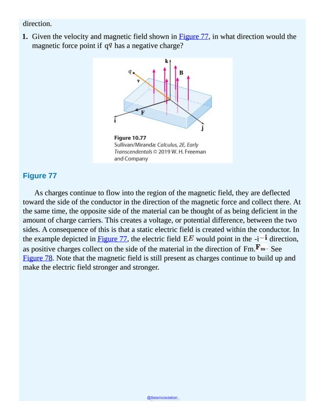
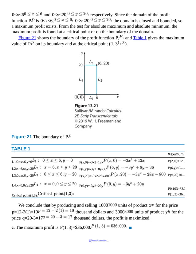
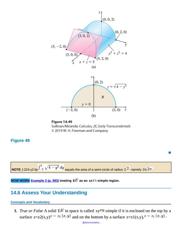
60. c. f(x+h)−f(x)
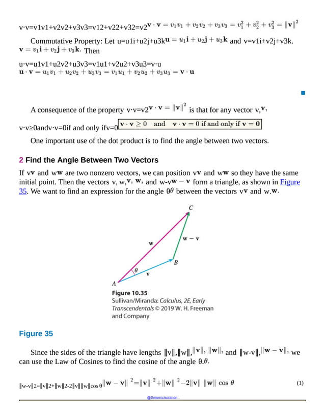
Solution a. f(5)=2⋅52−3⋅5=50−15=35
b. The function f(x)=2x2−3x gives us a rule to follow. To find f(x+h),
expand (x+h)2, multiply the result by 2, and then subtract the product
of 3 and (x+h).
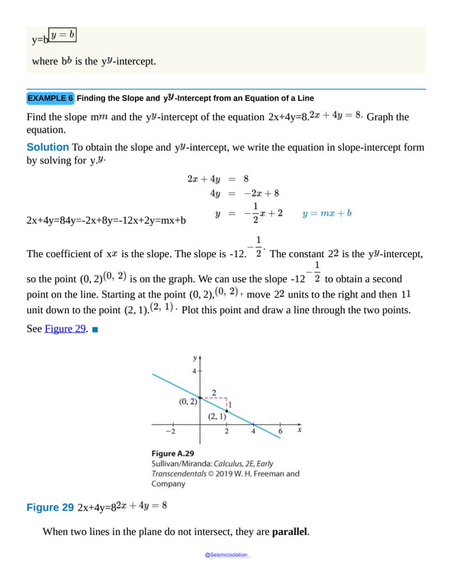
f
open
parenthesis
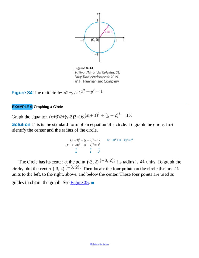
x
plus
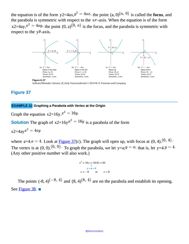
h
close
parenthesis
equals
2
open
parenthesis
x
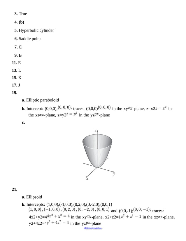
plus
h
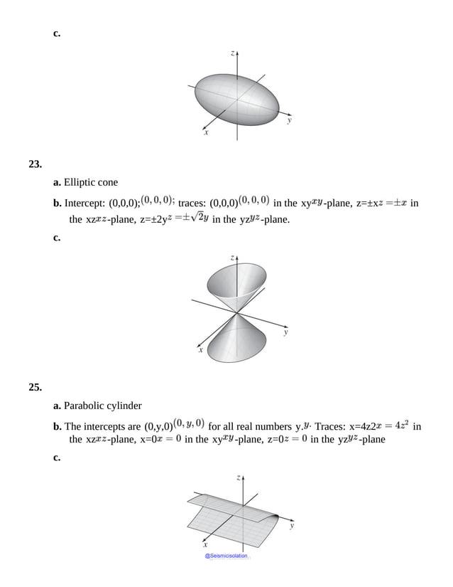
close
parenthesis
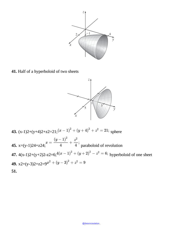
squared
minus
3
open
parenthesis
x
plus
h
close
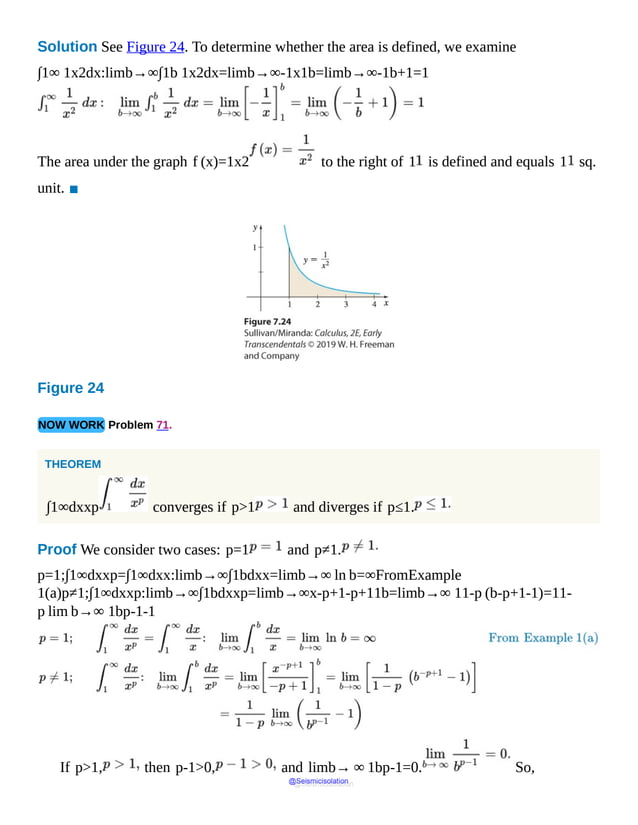
parenthesis
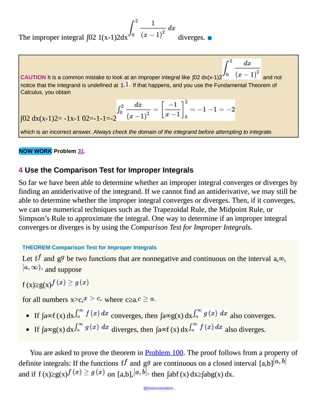
equals
c. f(x+h)−f(x)=[2x2+4hx+2h2−3x−3h]−[2x2−3x]=4hx+2h2−3h
▪
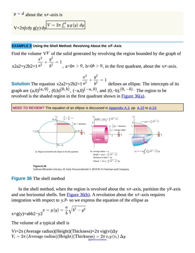
NOW WORK Problem 13.
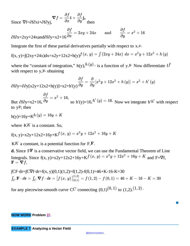
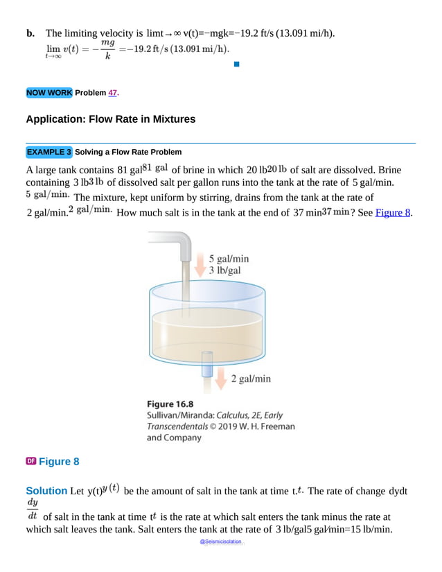
EXAMPLE 2 Finding the Amount of Gasoline in a Tank
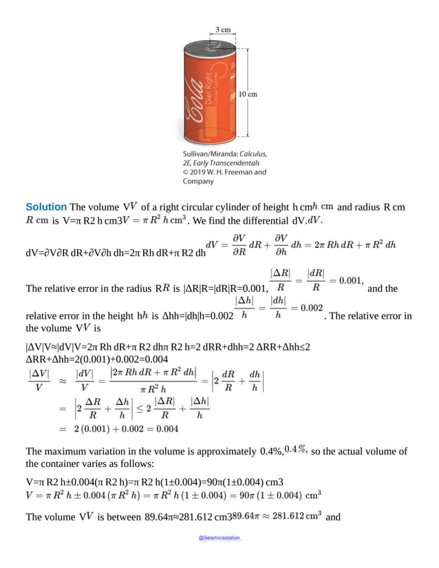
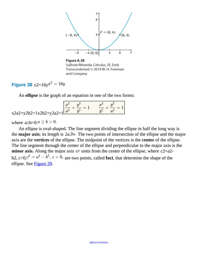
A Shell station stores its gasoline in an underground tank that is a right circular cylinder lying
on its side. The volume V of gasoline in the tank (in gallons) is given by the formula
V(h)=40h296h−0.608
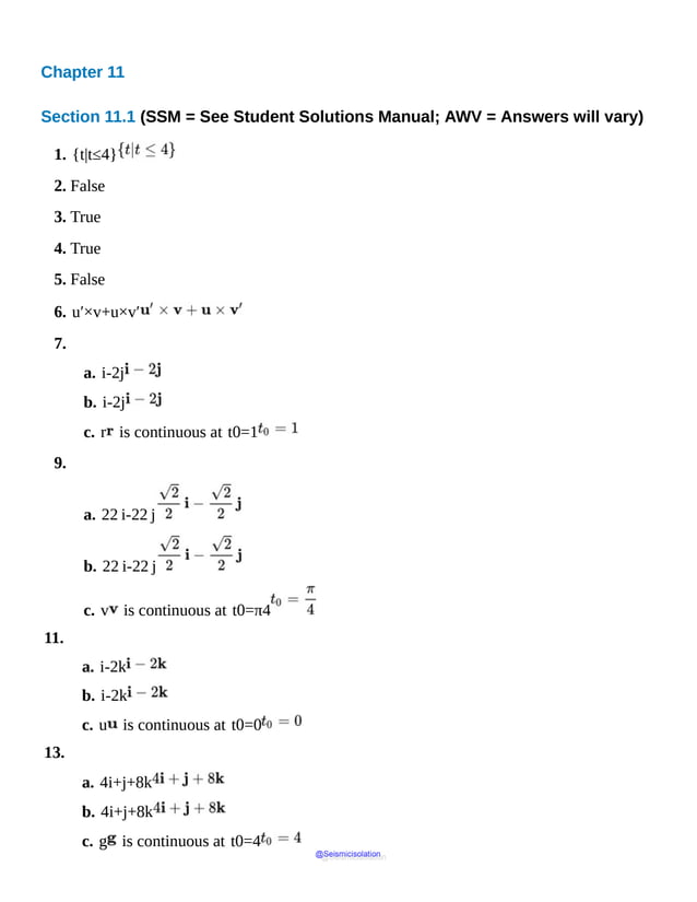
where h is the height (in inches) of the gasoline as measured on a depth stick. See Figure 5.
@Seismicisolation
@Seismicisolation

61. Figure 5
a. If h=12 inches, how many gallons of gasoline are in the tank?
b. If h=1 inch, how many gallons of gasoline are in the tank?
Solution a. We evaluate V when h=12.
V(12)=40⋅1229612−0.608=40⋅1448−0.608=57607.392≈15,660
There are about 15,660 gallons of gasoline in the tank when the height of the gasoline
in the tank is 12 inches.
b. Evaluate V when h=1.
V(1)=40⋅12961−0.608=4096−0.608=4095.392≈391
There are about 391 gallons of gasoline in the tank when the height of the gasoline in the
tank is 1 inch.
▪
Implicit Form of a Function
@Seismicisolation
@Seismicisolation

62. In general, a function f defined by an equation in x and y is given implicitly. If it is
possible to solve the equation for y in terms of x, then we write y=f(x) and say
the function is given explicitly. For example,
Implicit FormExplicit Formx2−y=6y=f(x)=x2−6 xy=4y=g(x)=4x
In calculus we sometimes deal with functions that are defined implicitly and that cannot
be expressed in explicit form. For example, if the function with independent variable x and
dependent variable y is defined by sin(xy)=xy−2y+cos x−sin y,
there is no method to solve for y and express the
function explicitly.
2 Find the Difference Quotient of a Function
An important concept in calculus involves working with a certain quotient. For a given
function y=f(x), the inputs x and x+h, h≠0, result in the images f(x)
and f(x+h). The quotient of their differences
f(x+h)−f(x)(x+h)−x=f(x+h)−f(x)h
with h≠0, is called the difference quotient of f at x.
DEFINITION Difference Quotient
The difference quotient of a function f at x is given by
f(x+h)−f(x)h h≠0
The difference quotient is used in calculus to define the derivative, which is used in
applications such as the velocity of an object and optimization of resources.
When finding a difference quotient, it is necessary to simplify the expression in order to
cancel the h in the denominator, as illustrated in the next example.
EXAMPLE 3 Finding the Difference Quotient of a Function
Find the difference quotient of each function.
@Seismicisolation
@Seismicisolation

63. a. f(x)=2x2−3x
b. f(x)=x
Solution
(a)
f
open
parenthesis
x
plus
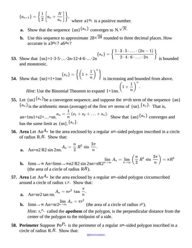
h
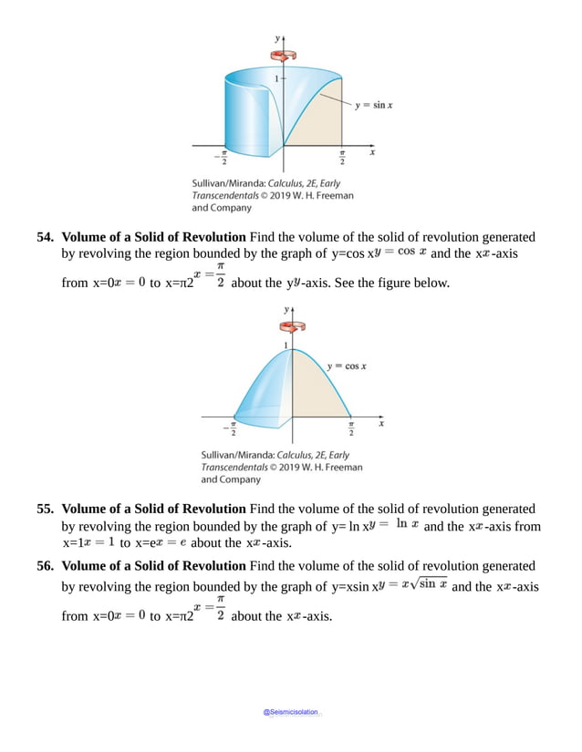
close
parenthesis
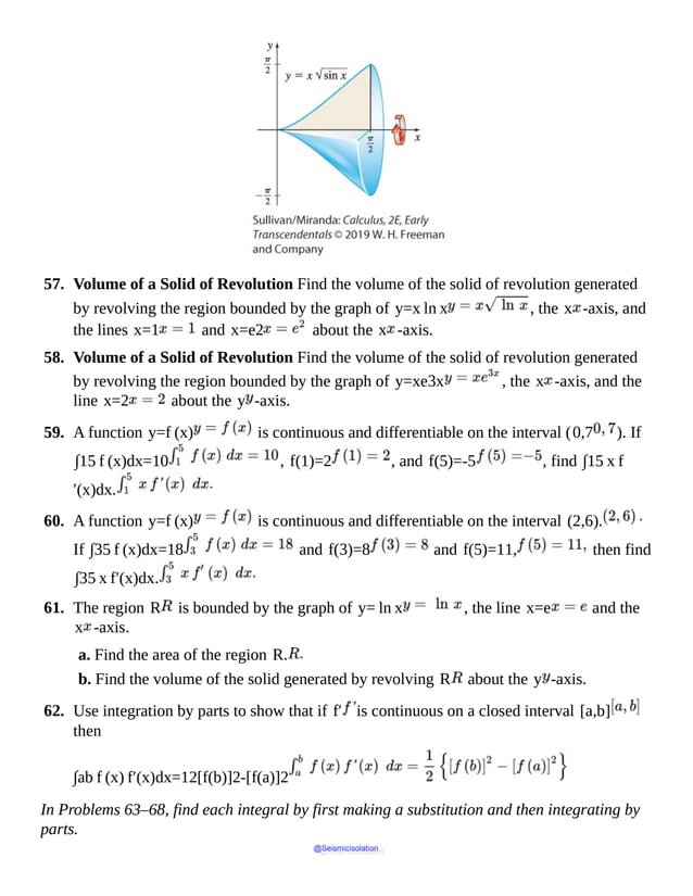
minus
f
of
x
all
over
▪
NOW WORK Problem 23.
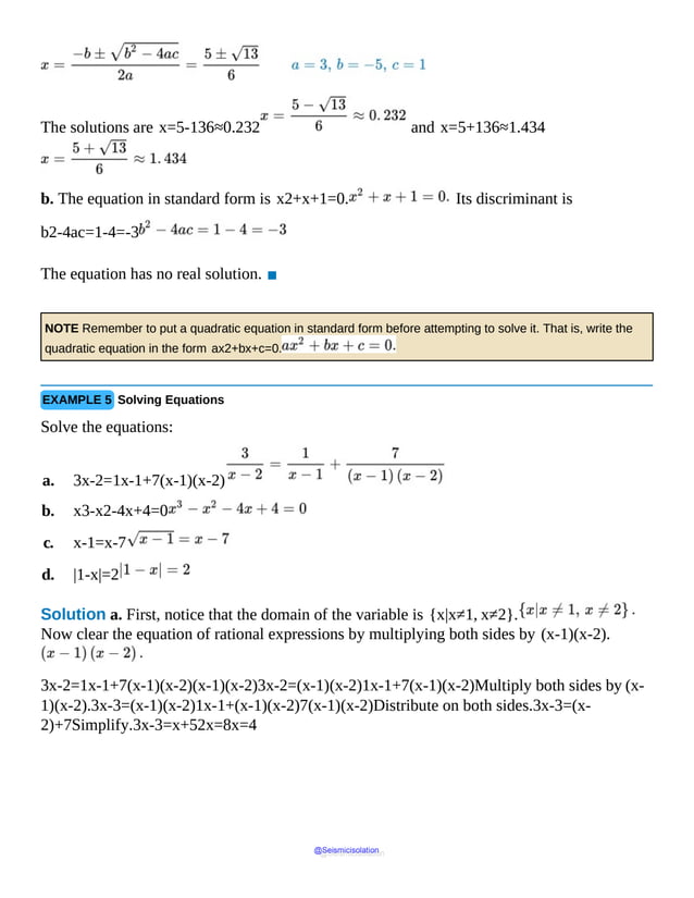
3 Find the Domain of a Function
In applications, the domain of a function is sometimes specified. For example, we might be
interested in the population of a city from 1990 to 2019. The domain of the function is time,
in years, and is restricted to the interval [1990, 2019]. Other times the domain is restricted by
the context of the function itself. For example, the volume V of a sphere, given by the
function V=43πR3, makes sense only if the radius R is greater than 0. But
often the domain of a function f is not specified; only the formula defining the function is
given. In such cases, the domain of f is the largest set of real numbers for which the value
@Seismicisolation
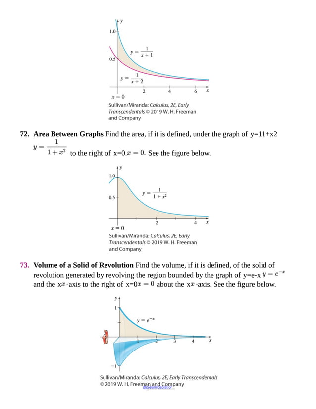
@Seismicisolation

64. f(x) is defined and is a real number.
EXAMPLE 4 Finding the Domain of a Function
Find the domain of each of the following functions:
a. f(x)=x2+5x
b. g(x)=3xx2−4
c. h(t)=4−3t
d. F(u)=5uu2−1
Solution a. Since f(x)=x2+5x is defined for any real number x, the
domain of f is the set of all real numbers.
b. Since division by zero is not defined, x2−4 cannot be 0, that is, x≠−2 and
x≠2. The function g(x)=3xx2−4 is defined for any real number except
x=−2 and x=2. So, the domain of g is the set of real numbers {x|x≠−2,x≠2}.
c. Since the square root of a negative number is not a real number, the value of 4−3t
must be nonnegative. The solution of the inequality 4−3t≥0 is t≤43, so the
domain of h is the set of real numbers t|t≤43 or the interval −∞,43.
NEED TO REVIEW? Solving inequalities is discussed in Appendix A.1, pp. A-6 to A-8.
NEED TO REVIEW? Interval notation is discussed in Appendix A.1, p. A-5.
d. Since the square root is in the denominator, the value of u2−1 must be not only
nonnegative, it also cannot equal zero. That is, u2−1>0. The solution of the
inequality u2−1>0 is the set of real numbers {u|u<−1}∪{u|u>1}
or the set (−∞,−1)∪(1,∞). ▪
If x is in the domain of a function f, we say that f is defined at x, or f(x)
@Seismicisolation
@Seismicisolation

65. exists. If x is not in the domain of f, we say that f is not defined at x, or f(x)
does not exist. The domain of a function is expressed using inequalities, interval notation, set
notation, or words, whichever is most convenient. Notice the various ways the domain was
expressed in the solution to Example 4.
NOW WORK Problem 17.
4 Identify the Graph of a Function
In applications, often a graph reveals the relationship between two variables more clearly
than an equation. For example, Table 2 shows the average price of gasoline at a particular gas
station in the United States (for the years 1985–2016 adjusted for inflation, based on 2014
dollars). If we plot these data using year as the independent variable and price as the
dependent variable, and then connect the points (year, price) we obtain Figure 6.
TABLE 2 Average Retail Price of Gasoline (2014 dollars)
Year Price Year Price Year Price
1985 2.55 1996 1.80 2007 3.19
1986 1.90 1997 1.76 2008 3.56
1987 1.89 1998 1.49 2009 2.58
1988 l.81 1999 1.61 2010 3.00
1989 1.87 2000 2.03 2011 3.69
1990 2.03 2001 1.90 2012 3.72
1991 1.91 2002 1.76 2013 3.54
1992 1.82 2003 1.99 2014 3.43
1993 1.74 2004 2.31 2015 2.74
1994 1.71 2005 2.74 2016 2.24
1995 1.72 2006 3.01
Source: U.S. Energy Information Administration
@Seismicisolation
@Seismicisolation

66. Figure 6 Graph of the average retail price of gasoline (2014 dollars).
Graph
of
price
in
dollars
versus
years
shows
an
up
down
moving
curving
beginning
at
price
2.50
in
1984
which
fluctuates
until
the
year
2002
after
The graph shows that for each date on the horizontal axis there is only one price on the
vertical axis. So, the graph represents a function, although the rule for determining the price
from the year is not given.
When a function is defined by an equation in x and y, the graph of the function is
the set of points (x,y) in the xy -plane that satisfy the equation.
NEED TO REVIEW? The graph of an equation is discussed in Appendix A.3, pp. A-16 to A-18.
But not every collection of points in the xy -plane represents the graph of a function.
Recall that a relation is a function only if each element x in the domain corresponds to
exactly one image y in the range. This means the graph of a function never contains two
points with the same x -coordinate and different y -coordinates. Compare the graphs in
Figures 7 and 8. In Figure 7, every number x is associated with exactly one number y,
but in Figure 8 some numbers x are associated with three numbers y. Figure 7 shows the
graph of a function; Figure 8 shows a graph that is not the graph of a function.
@Seismicisolation
@Seismicisolation

67. Figure 7 Function: Exactly one y for each x. Every vertical line intersects the graph in
at most one point.
Figure 8 Not a function: x=c has 3 y’s associated with it. The vertical line x=c
intersects the graph in three points.
For a graph to be a graph of a function, it must satisfy the Vertical-line Test.
THEOREM Vertical-line Test
A set of points in the xy -plane is the graph of a function if and only if every vertical line
intersects the graph in at most one point.
NOTE The phrase “if and only if” means the statements on each side of the phrase are equivalent. That is, they
have the same meaning.
EXAMPLE 5 Identifying the Graph of a Function
@Seismicisolation
@Seismicisolation

68. Which graphs in Figure 9 represent the graph of a function?
Figure 9
First
diagram
shows
a
parabolic
curve
of
function
y
equals
x
squared,
seconds
shows
an
S-
shaped
curve
of
function
y
equals
x
cubed,
third
shows
a
parabola
of
Solution The graphs in Figure 9(a), 9(b), and 9(e) are graphs of functions because every
vertical line intersects each graph in at most one point. The graphs in Figure 9(c) and 9(d) are
not graphs of functions because there is a vertical line that intersects each graph in more than
one point. ▪
NOW WORK Problems 31(a) and (b).
Notice that although the graph in Figure 9(e) represents a function, it looks different from
the graphs in (a) and (b). The graph consists of two pieces plus a point, and they are not
connected. Also notice that different equations describe different pieces of the graph.
Functions with graphs similar to the one in Figure 9(e) are called piecewise-defined
functions.
5 Analyze a Piecewise-Defined Function
Sometimes a function is defined differently on different parts of its domain. For example, the
absolute value function f(x)=|x | is actually defined by two equations: f(x)=x
if x≥0 and f(x)=−x if x<0. These equations are usually
combined into one expression as
f(x)=|x|=xifx≥0−xifx<0
Figure 10 shows the graph of the absolute value function. Notice that the graph of f satisfies
the Vertical-line Test.
@Seismicisolation
@Seismicisolation

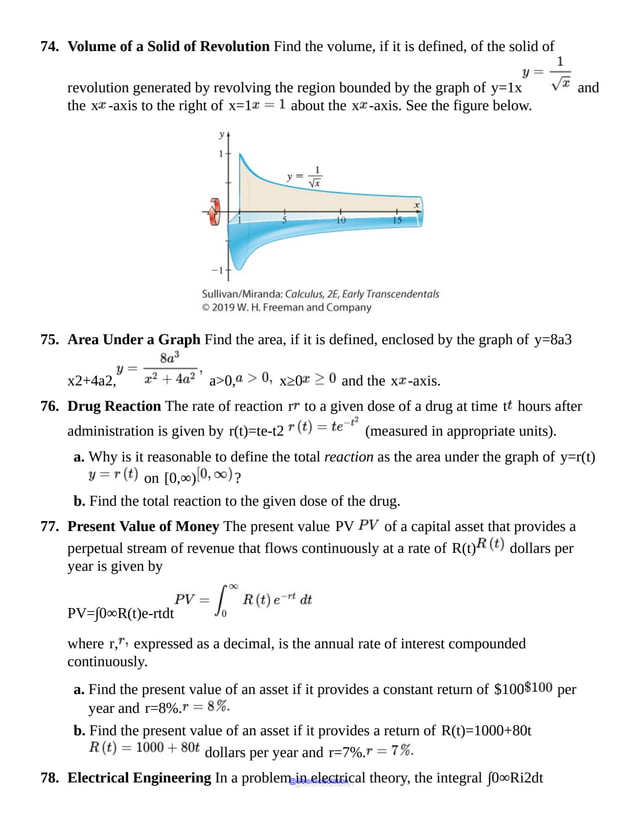
69. Figure 10 f(x)=|x |
When a function is defined by different equations on different parts of its domain, it is
called a piecewise-defined function.
EXAMPLE 6 Analyzing a Piecewise-Defined Function
The function f is defined as
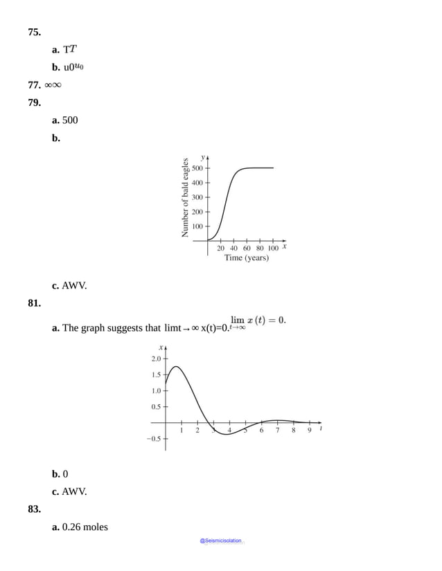
f(x)=0if x<010if 0≤x≤1000.2x−10 if x>100
a. Evaluate f(−1), f(100), and f(200).
b. Graph f.
c. Find the domain, range, and the x - and y -intercepts of f.
Solution a. f(−1)=0; f(100)=10; f(200)=0.2(200)−10=30
b. The graph of f consists of three pieces corresponding to each equation in the definition.
The graph is the horizontal line y=0 on the interval (−∞,0), the horizontal line
y=10 on the interval [0,100], and the line y=0.2x−10 on the
interval (100,∞), as shown in Figure 11.
@Seismicisolation
@Seismicisolation

70. Figure 11
Fuction
f
of
x
equals
0
if
x
is
lesser
than
0,
10
if
x
is
greater
than
or
equal
to
0
c. f is a piecewise-defined function. Look at the values that x can take on:
x<0,0≤x≤100,x>100. We conclude the domain of f is all real
numbers. The range of f is the number 0 and all real numbers greater than or equal to 10.
The x -intercepts are all the numbers in the interval (−∞,0) ; the y -intercept is
10. ▪
RECALL x -intercepts are numbers on the x -axis at which a graph touches or crosses the x -axis.
NOW WORK Problem 33.
6 Obtain Information From or About the Graph of a Function
The graph of a function provides a great deal of information about the function. Reading and
interpreting graphs is an essential skill for calculus.
EXAMPLE 7 Obtaining Information from the Graph of a Function
The graph of y=f(x) is given in Figure 12. (x might represent time and y might
represent the position of an object attached to a spring that has been compressed 4 units
above its at rest position and is then released. The object oscillates between 4 units above and
4 units below its at rest position.)
@Seismicisolation
@Seismicisolation

71. Figure 12
a. What are f(0), f3π2, and f(3π) ?
b. What is the domain of f ?
c. What is the range of f ?
d. List the intercepts of the graph.
e. How many times does the line y=2 intersect the graph of f ?
f. For what values of x does f(x)=−4 ?
g. For what values of x is f(x)>0 ?
Solution a. Since the point (0,4) is on the graph of f, the y -coordinate 4 is the
value of f at 0; that is, f(0)=4. Similarly, when x=3π2, then y=0,
so f3π2=0, and when x=3π, then y=−4, so f(3π)=−4.
b. The points on the graph of f have x -coordinates between 0 and 4π inclusive. The
domain of f is {x|0≤x≤4π} or the closed interval [0,4π].
c. Every point on the graph of f has a y -coordinate between −4 and 4 inclusive. The
range of f is {y|−4≤y≤4} or the closed interval [−4,4].
@Seismicisolation
@Seismicisolation

72. d. The intercepts of the graph of f are (0,4), π2,0, 3π2,0, 5π2,0,
and 7π2,0.
RECALL Intercepts are points at which a graph crosses or touches a coordinate axis.
e. Draw the graph of the line y=2 on the same set of coordinate axes as the graph of f.
The line intersects the graph of f four times.
f. Find points on the graph of f for which y=f(x)=−4 ; there are two such
points: (π,−4) and (3π,−4). So f(x)=−4 when x=π and
when x=3π.
g. f(x)>0 when the y -coordinate of a point (x,y) on the graph of f is
positive. This occurs when x is in the set 0,π2∪3π2,5π2∪7π2,4π.
▪
NOW WORK Problems 37, 39, 41, 43, 45, 47, and 49.
EXAMPLE 8 Obtaining Information About the Graph of a Function
Consider the function f(x)=x+1x+2.
a. What is the domain of f ?
b. Is the point 1,12 on the graph of f ?
c. If x=2, what is f(x) ? What is the corresponding point on the graph of f ?
d. If f(x)=2, what is x ? What is the corresponding point on the graph of f ?
e. What are the x -intercepts of the graph of f (if any)? What point(s) on the graph of f
correspond(s) to the x -intercept(s)?
Solution a. The domain of f consists of all real numbers except −2; that is, the set
{x|x≠−2}. The function is not defined at −2.
@Seismicisolation
@Seismicisolation

73. b. When x=1, then The point 1,23 is on the graph of f ; the
point 1,12 is not on the graph of f.
c. If x=2, then The point 2,34 is on the graph of f.
d. If f(x)=2, then x+1x+2=2. Solving for x, we find
x+1=2(x+2)x+1=2x+4x=−3
The point (−3,2) is on the graph of f.
e. The x -intercepts of the graph of f occur when y=0. That is, they are the solutions
of the equation f(x)=0. The x -intercepts are also called the real zeros or roots of
the function f.
The real zeros of the function f(x)=x+1x+2 satisfy the equation x+1=0,
so x=−1. The only x -intercept is −1, so the point (−1,0) is
on the graph of f. ▪
Figure 13 shows the graph of f.
@Seismicisolation
@Seismicisolation

74. Figure 13 f(x)=x+1x+2
NOW WORK Problems 55, 57, and 59.
7 Use Properties of Functions
One of the goals of calculus is to develop techniques for graphing functions. Here we review
some properties of functions that help obtain the graph of a function.
DEFINITION Even and Odd Functions
A function f is even if, for every number x in its domain, the number −x is also in
the domain and
f(−x)=f(x)
A function f is odd if, for every number x in its domain, the number −x is also in the
domain and
f(−x)=−f(x)
For example, f(x)=x2 is an even function since
f(−x)=(−x)2=x2=f(x)
@Seismicisolation
@Seismicisolation

75. Also, g(x)=x3 is an odd function since
g(−x)=(−x)3=−x3=−g(x)
See Figure 14 for the graph of f(x)=x2 and Figure 15 for the graph of g(x)=x3.
Notice that the graph of the even function f(x)=x2 is symmetric with
respect to the y -axis, and the graph of the odd function g(x)=x3 is symmetric
with respect to the origin.
Figure 14 The function f(x)=x2 is even. The graph of f is symmetric with
respect to the y -axis.
Figure 15 The function g(x)=x3. is odd. The graph of g is symmetric with
respect to the origin.
NEED TO REVIEW? Symmetry of graphs is discussed in Appendix A.3, pp. A-17 to A-18.
@Seismicisolation
@Seismicisolation

76. THEOREM Graphs of Even and Odd Functions
A function is even if and only if its graph is symmetric with respect to the y -axis.
A function is odd if and only if its graph is symmetric with respect to the origin.
EXAMPLE 9 Identifying Even and Odd Functions
Determine whether each of the following functions is even, odd, or neither. Then determine
whether its graph is symmetric with respect to the y -axis, the origin, or neither.
a. f(x)=x2−5
b. g(x)=4xx2−5
c. h(x)=5x3−13
d. F(x)=|x |
e. H(x)=x2+2x−1(x−5)2
Solution a. The domain of f is (−∞,∞), so for every number x in its domain,
−x is also in the domain. Replace x by −x and simplify.
f(−x)=(−x)2−5=x2−5=f(x)
Since f(−x)=f(x), the function f is even. So the graph of f is symmetric
with respect to the y -axis.
b. The domain of g is {x|x≠±5}, so for every number x in its domain, −x
is also in the domain. Replace x by −x and simplify.
g(−x)=4(−x)(−x)2−5=−4xx2−5=−g(x)
Since g(−x)=−g(x), the function g is odd. So the graph of g is symmetric
with respect to the origin.
c. The domain of h is (−∞,∞), so for every number x in its domain, −x is
also in the domain. Replace x by −x and simplify.
h(−x)=5(−x)3−13=−5x3−13=−(5x3+1)3=−5x3+13
@Seismicisolation
@Seismicisolation

77. Since h(−x)≠h(x) and h(−x)≠−h(x), the function h is
neither even nor odd. The graph of h is not symmetric with respect to the y -axis and not
symmetric with respect to the origin.
d. The domain of F is (−∞,∞), so for every number x in its domain, −x is
also in the domain. Replace x by −x and simplify.
F(−x)=|−x|=|−1|⋅|x|=|x|=F(x)
The function F is even. So the graph of F is symmetric with respect to the y -axis.
e. The domain of H is {x|x≠5}. The number x=−5 is in the domain of
H, but x=5 is not in the domain. So the function H is neither even nor odd, and
the graph of H is not symmetric with respect to the y -axis or the origin. ▪
NOW WORK Problem 61.
Another important property of a function is to know where it is increasing or decreasing.
DEFINITION
A function f is increasing on an interval I if, for any choice of x1 and x2 in I,
with x1<x2, then f(x1)<f(x2).
A function f is decreasing on an interval I if, for any choice of x1 and x2 in I,
with x1<x2, then f(x1)>f(x2).
A function f is constant on an interval I if, for all choices of x in I, the values of
f(x) are equal.
Notice in the definition for an increasing (decreasing) function f, the value f(x1)
is strictly less than (strictly greater than) the value f(x2). If a nonstrict inequality is
used, we obtain the definitions for nondecreasing and nonincreasing functions.
DEFINITION
A function f is nondecreasing on an interval I if, for any choice of x1 and x2 in I,
with x1<x2, then f(x1)≤f(x2).
A function f is nonincreasing on an interval I if, for any choice of x1 and x2
in I, with x1<x2, then f(x1)≥f(x2).
@Seismicisolation
@Seismicisolation

78. IN WORDS From left to right, the graph of an increasing function goes up, the graph of a decreasing function
goes down, and the graph of a constant function remains at a fixed height. From left to right, the graph of a
nondecreasing function never goes down, and the graph of a nonincreasing function never goes up. See Figure
16 on page 12.
Figure 16 illustrates the definitions. In Chapter 4 we use calculus to find where a function
is increasing or decreasing or is constant.
Figure 16
NOW WORK Problems 51 and 53.
8 Find the Average Rate of Change of a Function
The average rate of change of a function plays an important role in calculus. It provides
information about how a change in the independent variable x of a function y=f(x)
causes a change in the dependent variable y. We use the symbol Δx, read
“delta x, ” to represent the change in x and Δy to represent the change in y. Then by
forming the quotient ΔyΔx, we arrive at an average rate of change.
DEFINITION Average Rate of Change
If a and b, where a≠b, are in the domain of a function y=f(x), the
average rate of change of f from a to b is defined as
ΔyΔx=f(b)−f(a)b−aa≠b
NOTE ΔyΔx represents the change in y with respect to x.
EXAMPLE 10 Finding the Average Rate of Change
@Seismicisolation
@Seismicisolation

79. Find the average rate of change of f(x)=3x2:
a. From 1 to 3
b. From 1 to x, x≠1
Solution a. The average rate of change of f(x)=3x2 from 1 to 3 is
ΔyΔx=f(3)−f(1)3−1=27−33−1=242=12
See Figure 17.
Figure 17 f(x)=3x2
Notice that the average rate of change of f(x)=3x2 from 1 to 3 is the slope
of the line containing the points (1,3) and (3,27).
b. The average rate of change of f(x)=3x2 from 1 to x is
ΔyΔx=f(x)−f(1)x−1=3x2−3x−1=3(x2−1)x−1=3(x−1)(x+1)x−1=3(x+1)=3x+3
@Seismicisolation
@Seismicisolation

80. provided x≠1. ▪
NOW WORK Problem 65.
EXAMPLE 11 Analyzing a Cost Function
The weekly cost C, in dollars, of manufacturing x lightbulbs is
C(x)=7500+125x
a. Find the average rate of change of the weekly cost C of manufacturing from 100
to 101 lightbulbs.
b. Find the average rate of change of the weekly cost C of manufacturing from 1000
to 1001 lightbulbs.
c. Interpret the results from parts (a) and (b).
Solution a. The weekly cost of manufacturing 100 lightbulbs is
C(100)=7500+125⋅100=7500+12,500≈$7611.80
The weekly cost of manufacturing 101 lightbulbs is
C(101)=7500+125⋅101=7500+12,625≈$7612.36
The average rate of change of the weekly cost C from 100 to 101 is
ΔCΔx=C(101)−C(100)101−100≈7612.36−7611.801=$0.56
b. The weekly cost of manufacturing 1000 lightbulbs is
C(1000)=7500+125⋅1000=7500+125,000≈$7853.55
The weekly cost of manufacturing 1001 lightbulbs is
C(1001)=7500+125⋅1001=7500+125,125≈$7853.73
The average rate of change of the weekly cost C from 1000 to 1001 is
@Seismicisolation
@Seismicisolation

81. ΔCΔx=C(1001)−C(1000)1001−1000≈7853.73−7853.551=$0.18
c. Part (a) tells us that the unit cost of manufacturing the 101st lightbulb is $0.56. From
(b) we learn that the unit cost of manufacturing the 1001st lightbulb is only $0.18. The
unit cost of manufacturing the 1001st lightbulb is less than the unit cost of manufacturing the
101st lightbulb. ▪
NOW WORK Problem 73.
The Secant Line
The average rate of change of a function has an important geometric interpretation. Look at
the graph of y=f(x) in Figure 18 on page 14. Two points are labeled on the graph:
(a,f(a)) and (b,f(b)). The line containing these two points is called a
secant line. The slope of a secant line is
m
subscript
sec
equals
f
of
b
minus
f
of
a
all
over
b
minus
a
equals
f
open
Notice that the slope of a secant line equals the average rate of change of f from a to b
and also equals the difference quotient of f at a.
Figure 18 A secant line of the function y=f(x).
@Seismicisolation
@Seismicisolation

82. THEOREM Slope of a Secant Line
The average rate of change of a function f from a to b equals the slope of the secant
line containing the two points (a,f(a)) and (b,f(b)) on the graph of f.
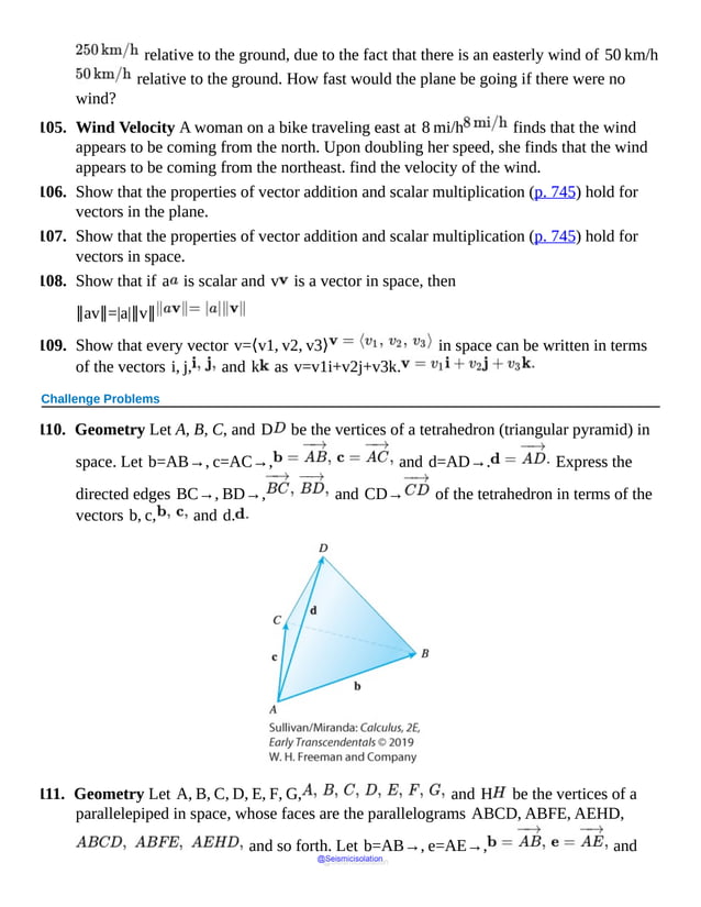
P.1 Assess Your Understanding
Concepts and Vocabulary
1. If f is a function defined by y=f(x), then x is called the __________
variable, and y is the __________ variable.
2. True or False The independent variable is sometimes referred to as the argument of the
function.
3. True or False If no domain is specified fora function f, then the domain of f is taken
to be the set of all real numbers.
4. True or False The domain of the function f(x)=3(x2−1)x−1 is {x|x≠
±1}.
5. True or False A function can have more than one y -intercept.
6. A set of points in the xy -plane is the graph of a function if and only if every
__________ line intersects the graph in at most one point.
7. If the point (5,−3) is on the graph of f, then f(__________)=__________.
8. Find a so that the point (−1,2) is on the graph of f(x)=ax2+4.
9. Multiple Choice A function f is [(a) increasing (b) decreasing (c) nonincreasing (d)
nondecreasing (e) constant] on an interval I if, for any choice of x1 and x2 in I,
with x1<x2, then f(x1)<f(x2).
10. Multiple Choice A function f is [(a) even (b) odd (c) neither even nor odd] if for every
number x in its domain, the number −x is also in the domain and f(−x)=f(x).
A function f is [(a) even (b) odd (c) neither even nor odd] if for every
number x in its domain, the number −x is also in the domain and f(−x)=−f(x).
11. True or False Even functions have graphs that are symmetric with respect to the origin.
@Seismicisolation
@Seismicisolation

83. 12. The average rate of change of f(x)=2x3−3 from 0 to 2 is __________.
Practice Problems
In Problems 13–16, for each function find:
a. f(0)
b. f(−x)
c. −f(x)
d. f(x+1)
e. f(x+h)
13. f(x)=3x2+2x−4
14. f(x)=xx2+1
15. f(x)=|x|+4
16. f(x)=3−x
In Problems 17–22, find the domain of each function.
17. f(x)=x3−1
18. f(x)=xx2+1
19. v(t)=t2−9
20. g(x)=2x−1
21. h(x)=x+2x3−4x
22. s(t)=t+1t−5
In Problems 23–28, find the difference quotient of f . That is, find
f(x+h)−f(x)h, h≠0
@Seismicisolation
@Seismicisolation

84. 23. f(x)=−3x+1
24. f(x)=1x+3
25. f(x)=x+7
26. f(x)=2x+7
27. f(x)=x2+2x
28. f(x)=(2x+3)2
In Problems 29–32, determine whether the graph is that of a function by using the Vertical-
line Test. If it is, use the graph to find
a. the domain and range
b. the intercepts, if any
c. any symmetry with respect to the x -axis, y -axis, or the origin.
29.
30.
@Seismicisolation
@Seismicisolation

85. 31.
32.
In Problems 33–36, for each piecewise-defined function:
a. Find f(−1), f(0), f(1), and f(8).
@Seismicisolation
@Seismicisolation

86. b. Graph f.
c. Find the domain, range, and intercepts of f.
33. f(x)=x+3if−2≤x<15ifx=1−x+2ifx>1
34. f(x)=2x+5if−3≤x<0−3ifx=0−5xifx>0
35. f(x)=1+xifx<0x2ifx≥0
36. f(x)=1xifx<0x3ifx≥0
In Problems 37–54, use the graph of the function f to answer the questions.
37. Find f(0) and f(−6).
38. Is f(3) positive or negative?
@Seismicisolation
@Seismicisolation

87. 39. Is f(−4) positive or negative?
40. For what values of x is f(x)=0 ?
41. For what values of x is f(x)>0 ?
42. What is the domain of f ?
43. What is the range of f ?
44. What are the x -intercepts?
45. What is the y -intercept?
46. How often does the line y=12 intersect the graph?
47. How often does the line x=5 intersect the graph?
48. For what values of x does f(x)=3 ?
49. For what values of x does f(x)=−2 ?
50. On what interval(s) is the function f increasing?
51. On what interval(s) is the function f decreasing?
52. On what interval(s) is the function f constant?
53. On what interval(s) is the function f nonincreasing?
54. On what interval(s) is the function f nondecreasing?
In Problems 55–60, answer the questions about the function
g(x)=x+2x−6
55. What is the domain of g ?
56. Is the point (3,14) on the graph of g ?
57. If x=4, what is g(x) ? What is the corresponding point on the graph of g ?
58. If g(x)=2, what is x ? What is (are) the corresponding point(s) on the graph
of g ?
59. List the x -intercepts, if any, of the graph of g.
60. What is the y -intercept, if there is one, of the graph of g ?
In Problems 61–64, determine whether the function is even, odd, or neither. Then determine
@Seismicisolation
@Seismicisolation

88. whether its graph is symmetric with respect to the y -axis, the origin, or neither.
61. h(x)=xx2−1
62. f(x)=3x2+13
63. G(x)=x
64. F(x)=2x| x |
65. Find the average rate of change of f(x)=−2x2+4:
a. From 1 to 2
b. From 1 to 3
c. From 1 to 4
d. From 1 to x, x≠1
66. Find the average rate of change of s(t)=20−0.8t2:
a. From 1 to 4
b. From 1 to 3
c. From 1 to 2
d. From 1 to t, t≠1
In Problems 67–72, the graph of a piecewise-defined function is given. Write a definition for
each piecewise-defined function. Then state the domain and the range of the function.
67.
@Seismicisolation
@Seismicisolation

89. 68.
69.
70.
@Seismicisolation
@Seismicisolation

90. 71.
Function
y
equals
minus
x
squared
decreases
exponentially
from
72.
@Seismicisolation
@Seismicisolation

91. Function
y
equals
x
squared
minus
1
decreases
exponentially
from
(minus
3,
8)
to
(0,
minus
1)
and
a
function
y
equals
x
cubed
increases
exponentially
73. The monthly cost C, in dollars, of manufacturing x road bikes is given by the
function
C(x)=0.004x3−0.6x2+250x+100,500
a. Find the average rate of change of the cost C of manufacturing from 100 to
101 road bikes.
b. Find the average rate of change of the cost C of manufacturing from 500 to 501
road bikes.
c. Interpret the results from parts (a) and (b) in the context of the problem.
74. The graph in the right column represents the distance d (in miles) that Kevin was from
home as a function of time t (in hours). Answer the questions by referring to the graph.
In parts (a)–(g), how many hours elapsed and how far was Kevin from home during this
time?
a. From t=0 to t=2
b. From t=2 to t=2.5
c. From t=2.5 to t=2.8
d. From t=2.8 to t=3
e. From t=3 to t=3.9
f. From t=3.9 to t=4.2
g. From t=4.2 to t=5.3
h. What is the farthest distance that Kevin was from home?
@Seismicisolation
@Seismicisolation

92. i. How many times did Kevin return home?
Graph
increases
steeply
up
to
point
(2,
3)
and
remains
constant
up
to
x
value
2.5,
then
decreases
steeply
up
to
point
(2.8,
0)
and
remains
constant
up
to
75. Population as a Function of Age The function
P(a)=0.014a2−5.073a+327.287
represents the population P (in millions) of Americans that were a years of age or
older in 2012.
a. Identify the independent and dependent variables.
b. Evaluate P(20). Interpret P(20) in the context of this problem.
c. Evaluate P(0). Interpret P(0) in the context of this problem.
Source: U.S. Census Bureau
1. = NOW WORK problem
= Graphing technology recommended
= Computer Algebra System recommended
* The sets X and Y will usually be sets of real numbers, defining a real function. The two sets could also be sets of complex
numbers, defining a complex function, or X could be a set of real numbers and Y a set of vectors, defining a vector-valued
function. In the broad definition, X and Y can be any two sets.
@Seismicisolation
@Seismicisolation

93. P.2 Library of Functions; Mathematical Modeling
OBJECTIVES When you finish this section, you should be able to:
1 Develop a library of functions
2 Analyze a polynomial function and its graph
3 Find the domain and the intercepts of a rational function
4 Construct a mathematical model
When a collection of functions have common properties, they can be “grouped together” as
belonging to a class of functions. Polynomial functions, exponential functions, and
trigonometric functions are examples of classes of functions. As we investigate principles of
calculus, we will find that often a principle applies to all functions in a class in the same way.
1 Develop a Library of Functions
Most of the functions in this section will be familiar to you; several might be new. Although
the list may seem familiar, pay special attention to the domain of each function and to its
properties, particularly to the shape of each graph. Knowledge of these graphs lays the
foundation for later graphing techniques.
Constant Function f(x)=AA is a real number
The domain of a constant function is the set of all real numbers; its range is the single
number A. The graph of a constant function is a horizontal line whose y -intercept is A;
it has no x -intercept if A≠0. A constant function is an even function. See Figure
19.
@Seismicisolation
@Seismicisolation

94. Figure 19 f(x)=A
Identity Function f(x)=x
The domain and the range of the identity function are the set of all real numbers. Its
graph is the line through the origin whose slope is m=1. Its only intercept is (0,0).
The identity function is an odd function; its graph is symmetric with respect to the
origin. It is increasing over its domain. See Figure 20.
Figure 20 f(x)=x
Notice that the graph of f(x)=x bisects quadrants I and III.
The graphs of both the constant function and the identity function are straight lines.
These functions belong to the class of linear functions:
Linear Functions f(x)=mx+bm and b are real numbers
@Seismicisolation
@Seismicisolation

95. NEED TO REVIEW? Equations of lines are discussed in Appendix A.3, pp. A-18 to A-20.
The domain of a linear function is the set of all real numbers. The graph of a linear
function is a line with slope m and y -intercept b. If m>0, f is an increasing
function, and if m<0, f is a decreasing function. If m=0, then f is a constant
function, and its graph is the horizontal line, y=b. See Figure 21.
Figure 21
First
diagram
shows
a
line
having
positive
slope
depicting
increasing
function,
second
diagram
shows
a
line
having
negative
slope
depicting
decreasing
function
and
In a power function, the independent variable x is raised to a power.
Power Functions f(x)=xaa is a real number
Below we examine power functions f(x)=xn, where n≥1 is a positive
integer. The domain of these power functions is the set of all real numbers. The only intercept
of their graph is the point (0,0).
If f is a power function and n is a positive odd integer, then f is an odd function
whose range is the set of all real numbers and the graph of f is symmetric with respect to
the origin. The points (−1,−1), (0,0), and (1,1) are on the graph of f.
As x becomes unbounded in the negative direction, f also becomes unbounded in the
negative direction. Similarly, as x becomes unbounded in the positive direction, f also
becomes unbounded in the positive direction. The function f is increasing over its domain.
The graphs of several odd power functions are given in Figure 22.
@Seismicisolation
@Seismicisolation

96. Figure 22
First
diagram
shows
a
line
passing
through
the
origin
depicting
the
function
f
of
x
equals
x,
second
and
third
diagrams
show
an
S-
curve
symmetric
to
origin
depicting
the
functions
If f is a power function and n is a positive even integer, then f is an even function
whose range is {y|y≥0}. The graph of f is symmetric with respect to the y -axis.
The points (−1,1), (0,0), and (1,1) are on the graph of f. As x
becomes unbounded in either the negative direction or the positive direction, f becomes
unbounded in the positive direction. The function is decreasing on the interval (−∞,0]
and is increasing on the interval [0,∞).
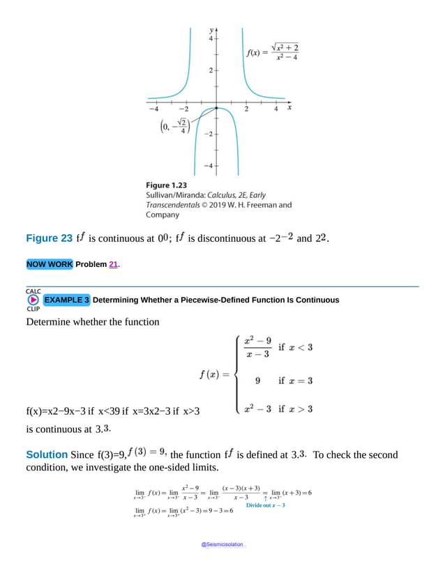
The graphs of several even power functions are shown in Figure 23.
Figure 23
First
diagram
shows
a
parabolic
curve
symmetric
to
y-
axis
depicting
the
Look closely at Figures 22 and 23. As the integer exponent n increases, the graph of f
is flatter (closer to the x -axis) when x is in the interval (−1,1) and steeper when x
is in interval (−∞,−1) or (1,∞).
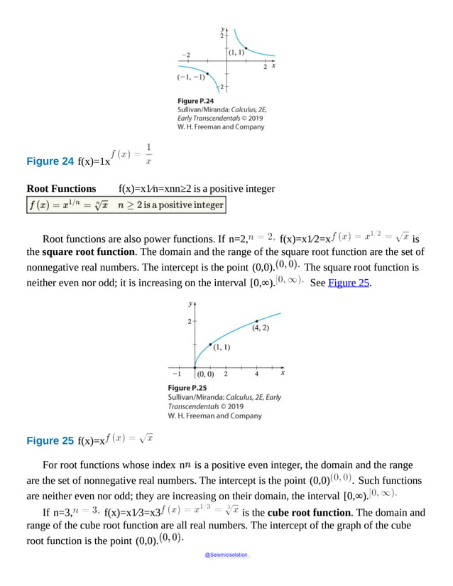
The Reciprocal Function f(x)=1x
The domain and the range of the reciprocal function (the power function f(x)=xa,
a=−1 ) are the set of all nonzero real numbers. The graph has no
intercepts. The reciprocal function is an odd function so the graph is symmetric with respect
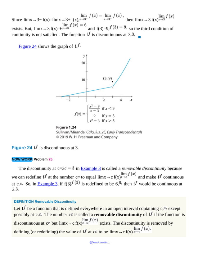
to the origin. The function is decreasing on (−∞,0) and on (0,∞). See Figure
24.
@Seismicisolation
@Seismicisolation

97. Figure 24 f(x)=1x
Root Functions f(x)=x1⁄n=xnn≥2 is a positive integer
Root functions are also power functions. If n=2, f(x)=x1⁄2=x is
the square root function. The domain and the range of the square root function are the set of
nonnegative real numbers. The intercept is the point (0,0). The square root function is
neither even nor odd; it is increasing on the interval [0,∞). See Figure 25.
Figure 25 f(x)=x
For root functions whose index n is a positive even integer, the domain and the range
are the set of nonnegative real numbers. The intercept is the point (0,0) . Such functions
are neither even nor odd; they are increasing on their domain, the interval [0,∞).
If n=3, f(x)=x1⁄3=x3 is the cube root function. The domain and
range of the cube root function are all real numbers. The intercept of the graph of the cube
root function is the point (0,0).
@Seismicisolation
@Seismicisolation

98. Because f(−x)=−x3=−x3=−f(x), the cube root function is
odd. Its graph is symmetric with respect to the origin. The cube root function is increasing on
the interval (−∞,∞). See Figure 26.
Figure 26 f(x)=x3
The
graph
passes
through
the
points
(0,
0),
(1
by
8,
1
by
2),
(1,
1),
(2,
cube
root
of
2),
(minus
For root functions whose index n is a positive odd integer, the domain and the range are
the set of all real numbers. The intercept is the point (0,0). Such functions are odd so
their graphs are symmetric with respect to the origin. They are increasing on the interval
(−∞,∞).
Absolute Value Function f(x)=|x |
The absolute value function is defined as the piecewise-defined function
f(x)=|x|=xifx≥0−xifx<0
or as the function
f(x)=|x|=x2
The domain of the absolute value function is the set of all real numbers. The range is the set
of nonnegative real numbers. The intercept of the graph of f is the point (0,0).
Because f(−x)=|−x|=|x|=f(x), the absolute value function is even.
Its graph is symmetric with respect to the y -axis. See Figure 27.
@Seismicisolation
@Seismicisolation

99. Figure 27 f(x)=|x |
Graph
passes
through
the
points
(minus
2,
2),
(minus
1,
1),
(0,
0),
(1,
1)
and
(2,
2).
NOW WORK Problems 11 and 15.
The floor function, also known as the greatest integer function, is defined as the largest
integer less than or equal to x:
f(x)=⌊x⌋=largest integer less than or equal to x
The domain of the floor function ⌊x⌋ is the set of all real numbers; the range is the set of
all integers. The y -intercept of ⌊x⌋ is 0, and the x -intercepts are the numbers in the
interval [0,1). The floor function is constant on every interval of the form [k,k+1),
where k is an integer, and is nondecreasing on its domain. See Figure 28.
Figure 28 f(x)=⌊x⌋
@Seismicisolation
@Seismicisolation

100. The
function
is
discontinuous
at
the
points
(minus
2,
minus
2),
(minus
1,
minus
1),
(0,
0),
(1,
1),
(2,
2),
and
(3,
3).
The
lines
contain
holes
at
the
left
end.
IN WORDS The floor function can be thought of as the “rounding down” function. The ceiling function can be
thought of as the “rounding up” function.
The ceiling function is defined as the smallest integer greater than or equal to x:
f(x)=⌈x⌉=smallest integer greater than or equal to x
The domain of the ceiling function ⌈x⌉ is the set of all real numbers; the range is the set
of integers. The y -intercept of ⌈x⌉ is 0, and the x -intercepts are the numbers in the
interval (−1,0]. The ceiling function is constant on every interval of the form
(k,k+1], where k is an integer, and is nondecreasing on its domain. See Figure
29.
Figure 29 f(x)=⌈x⌉
The
function
is
discontinuous
at
(minus
1,
minus
1),
(0,
For example, for the floor function, ⌊3⌋=3 and ⌊2.9⌋=2, but for the
ceiling function, ⌈3⌉=3 and ⌈2.9⌉=3.
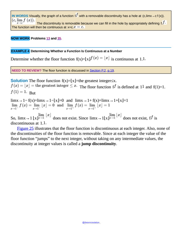
The floor and ceiling functions are examples of step functions. At each integer the
function has a discontinuity. That is, at integers the function jumps from one value to another
without taking on any of the intermediate values.
2 Analyze a Polynomial Function and Its Graph
A monomial is a function of the form y=axn, where a≠0 is a real number and
n≥0 is an integer. Polynomial functions are formed by adding a finite number of
monomials. @Seismicisolation
@Seismicisolation

101. DEFINITION Polynomial Function
A polynomial function is a function of the form
f(x)=anxn+an−1xn−1+⋯+a1x+a0
where an, an−1,…,a1, a0 are real numbers and n is a nonnegative
integer. The domain of a polynomial function is the set of all real numbers.
If an≠0, then an is called the leading coefficient of f, and the polynomial
has degree n.
The constant function f(x)=A, where A≠0, is a polynomial function of
degree 0. The constant function f(x)=0 is the zero polynomial function and has
no degree. Its graph is a horizontal line containing the point (0,0).
If the degree of a polynomial function is 1, then it is a linear function of the form
f(x)=mx+b, where m≠0. The graph of a linear function is a straight
line with slope m and y -intercept b.
Any polynomial function f of degree 2 can be written in the form
f(x)=ax2+bx+c
where a, b, and c are constants and a≠0. The square function f(x)=x2
is a polynomial function of degree 2. Polynomial functions of degree 2 are also called
quadratic functions. The graph of a quadratic function is known as a parabola and is
symmetric about its axis of symmetry, the vertical line x=−b2a. Figure 30 shows
the graphs of typical parabolas and their axes of symmetry. The x -intercepts, if any, of a
quadratic function satisfy the quadratic equation ax2+bx+c=0.
@Seismicisolation
@Seismicisolation

102. Figure 30
First
diagram
shows
a
parabola
at
first
and
second
quadrants
with
one
x-
intercept,
second
diagram
shows
a
parabola
at
first,
second
and
fourth
quadrants
with
two
x
intercepts,
NEED TO REVIEW? Quadratic equations and the discriminant are discussed in Appendix A.1, pp. A-3 to A-4.
Graphs of polynomial functions have many properties in common.
The zeros of a polynomial function f give insight into the graph of f. If r is a real
zero of a polynomial function f, then r is an x -intercept of the graph of f, and (x−r)
is a factor of f.
If (x−r) occurs more than once in the factored form of f, then r is called a
repeated or multiple zero of f. In particular, if (x−r)m is a factor of f, but (x
−r)m+1, where m≥1 is an integer, is not a factor of f, then r is called a
zero of multiplicity m of f. When the multiplicity of a zero r is an even integer, the
graph of f will touch (but not cross) the x -axis at r ; when the multiplicity of r is an odd
integer, then the graph of f will cross the x -axis at r. As Figure 31 illustrates, when the
graph crosses the x -axis, the sign of f(x) changes, and when the graph touches the x -
axis, the sign of f(x) remains the same.
@Seismicisolation
@Seismicisolation

103. Figure 31 The graph of a polynomial function.
Graph
is
below
the
x-
axis
when
the
function
f
of
x
is
less
than
0,
above
the
x-
axis
when
f
is
greater
than
0,
NOTE Finding the zeros of a polynomial function f is easy if f is linear, quadratic, or in factored form.
Otherwise, finding the zeros can be diffcult.
EXAMPLE 1 Analyzing the Graph of a Polynomial Function
For the polynomial function f(x)=x2(x−4)(x+1):
a. Find the x - and y -intercepts of the graph of f.
b. Determine whether the graph crosses or touches the x -axis at each x -intercept.
c. Plot at least one point to the left and right of each x -intercept and connect the points to
obtain the graph.
Solution a. The y -intercept is f(0)=0. The x -intercepts are the zeros of the
function: 0, 4, and −1.
b. 0 is a zero of multiplicity 2 ; the graph of f will touch the x -axis at 0. The
numbers 4 and −1 are zeros of multiplicity 1 ; the graph of f will cross the x -axis at
4 and −1.
c. Since f(−2)=24, f−12=−916, f(2)=−24, and
f(5)=150, the points (−2,24), −12,−916, (2,−24),
and (5,150) are on the graph. See Figure 32. ▪
@Seismicisolation
@Seismicisolation

104. Figure 32 f(x)=x2(x−4)(x+1)
=x4−3x3−4x2
Graph
passes
through
the
points
(minus
2,
24),
(minus
1,
0),
(minus
1
by
2,
minus
9
by
16),
(0,
0),
The behavior of the graph of a function for large values of x, either positive or
negative, is referred to as its end behavior.
For large values of x, either positive or negative, the graph of the polynomial function
f(x)=anxn+an−1xn−1+⋯+a1x+a0an≠0
resembles the graph of the power function
y=anxn
For example, the end behavior of the graph of the polynomial function f(x)=x4−3x3−4x2,
shown in Figure 32, resembles the graph of y=x4.
As another example, if f(x)=−2x3+5x2+x−4, then the graph
of f will behave like the graph of y=−2x3 for very large values of x, either
positive or negative. We can see that the graphs of f and y=−2x3 “behave” the
same by considering Table 3 and Figure 33.
TABLE 3 @Seismicisolation
@Seismicisolation

105. TABLE 3
x f(x) y=−2x3
10 −1494 −2000
100 −1,949,904 −2,000,000
500 −248,749,504 −250,000,000
1000 −1,994,999,004 −2,000,000,000
Figure 33
NOW WORK Problem 21.
3 Find the Domain and the Intercepts of a Rational Function
The quotient of two polynomial functions p and q is called a rational function.
DEFINITION Rational Function
A rational function is a function of the form
R(x)=p(x)q(x)
where p and q are polynomial functions and q is not the zero polynomial. The domain
of R is the set of all real numbers, except those for which the denominator q is 0.
If R(x)=p(x)q(x) is a rational function, the real zeros, if any, of the
@Seismicisolation
@Seismicisolation

106. numerator, which are also in the domain of R, are the x -intercepts of the graph of R.
EXAMPLE 2 Finding the Domain and the Intercepts of a Rational Function
Find the domain and the intercepts (if any) of each rational function:
a. R(x)=2x2−4x2−4
b. R(x)=xx2+1
c. R(x)=x2−1x−1
Solution a. The domain of R(x)=2x2−4x2−4 is {x|x≠−2;x≠2}.
Since 0 is in the domain of R and R(0)=1, the y -intercept
is 1. The zeros of R are solutions of the equation 2x2−4=0 or x2=2.
Since −2 and 2 are in the domain of R, the x -intercepts are −2 and 2.
b. The domain of R(x)=xx2+1 is the set of all real numbers. Since 0 is in
the domain of R and R(0)=0, the y -intercept is 0, and the x -intercept is also
0.
c. The domain of R(x)=x2−1x−1 is {x|x≠1}. Since 0 is in the
domain of R and R(0)=1, the y -intercept is 1. The x -intercept(s), if any,
satisfy the equation
x2−1=0x2=1x=−1 or x=1
Since 1 is not in the domain of R, the only x -intercept is −1. ▪
Figure 34 shows the graphs of R(x)=x2−1x−1 and f(x)=x+1.
Notice the “hole” in the graph of R at the point (1,2). Also,
R(x)=x2−1x−1 and f(x)=x+1 are not the same function: their
@Seismicisolation
@Seismicisolation

107. domains are different. The domain of R is {x|x≠1} and the domain of f is the
set of all real numbers.
Figure 34
First
graph
depicts
the
function
R
of
x
equals
x
squared
minus
1
by
x
minus
1
which
has
NOW WORK Problem 27.
Algebraic Functions
Every function discussed so far belongs to a broad class of functions called algebraic
functions. A function f that can be expressed in terms of sums, differences, products,
quotients, powers, or roots of polynomial functions is an algebraic function. For example, the
function f defined by
f(x)=3x3−x2(x+1)4⁄3x4+2
is an algebraic function. Functions that are not algebraic are called transcendental
functions. Examples of transcendental functions include the trigonometric functions,
exponential functions, and logarithmic functions, which are discussed later.
4 Construct a Mathematical Model
Problems in engineering and the sciences often can by solved using mathematical models
that involve functions. To build a model, verbal descriptions must be translated into the
@Seismicisolation
@Seismicisolation

108. language of mathematics by assigning symbols to represent the independent and dependent
variables and then finding a function that relates the variables.
EXAMPLE 3 Constructing a Model from a Verbal Description
A liquid is poured into a container in the shape of a right circular cone with radius 4 meters
and height 16 meters, as shown in Figure 35. Express the volume V of the liquid as a
function of the height h of the liquid.
Figure 35
Solution The formula for the volume of a right circular cone of radius r and height h is
V=13πr2h
The volume depends on two variables, r and h. To express V as a function of h only,
we use the fact that a cross section of the cone and the liquid form two similar triangles. See
Figure 36.
@Seismicisolation
@Seismicisolation

109. Figure 36
Corresponding sides of similar triangles are in proportion. Since the cone’s radius is 4
meters and its height is 16 meters, we have
rh=416=14r=14 h
Then
V
equals
1
over
3
times
pi
r
squared
h
equals
1
over
So V=V(h)=148πh3 expresses the volume V as a function of the
height of the liquid. Since h is measured in meters, V will be expressed in cubic meters.
▪
NEED TO REVIEW? Similar triangles and geometry formulas are discussed in Appendix A.2, pp. A-13 to A-15.
NOW WORK Problem 29.
In many applications, data are collected and are used to build the mathematical model. If
the data involve two variables, the first step is to plot ordered pairs using rectangular
coordinates. The resulting graph is called a scatter plot.
Scatter plots are used to help suggest the type of relation that exists between the two
@Seismicisolation
@Seismicisolation

110. variables. Once the general shape of the relation is recognized, a function can be chosen
whose graph closely resembles the shape in the scatter plot.
EXAMPLE 4 Identifying the Shape of a Scatter Plot
Determine whether you would model the relation between the two variables shown in each
scatter plot in Figure 37 with a linear function or a quadratic function.
Figure 37
Solution For each scatter plot, we choose a function whose graph closely resembles the
shape of the scatter plot. See Figure 38.
Figure 38
EXAMPLE 5 Building a Function from Data
The data shown in Table 4 measure crop yield for various amounts of fertilizer:
a. Draw a scatter plot of the data and determine a possible type of relation that may exist
between the two variables.
b. Use technology to find the function of best fit to these data.
TABLE 4
Plot
Fertilizer, x (Pounds/
100 ft2 )
Yield (Bushels)
1 0 4
2 0 6
3 5 10
4 5 7
5 10 12
@Seismicisolation
@Seismicisolation

111. 6 10 10
7 15 15
8 15 17
9 20 18
10 20 21
11 25 20
12 25 21
13 30 21
14 30 22
15 35 21
16 35 20
17 40 19
18 40 19
Solution a. Figure 39 shows the data and a scatter plot. The scatter plot suggests the graph
of a quadratic function.
b. The graphing calculator screen in Figure 40 shows that the quadratic function of best fit is
Y(x)=−0.017x2+1.077x+3.894
where x represents the amount of fertilizer used and Y represents crop yield. The graph
of the quadratic model is illustrated in Figure 41.
Figure 39
Figure 40
@Seismicisolation
@Seismicisolation

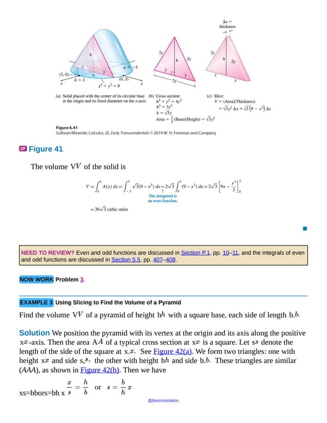
112. Figure 41
▪
NOW WORK Problem 31.
P.2 Assess Your Understanding
Concepts and Vocabulary
1. Multiple Choice The function f(x)=x2 is [(a) increasing (b) decreasing (c)
neither] on the interval [0,∞).
2. True or False The floor function f(x)=⌊x⌋ is an example of a step function.
3. True or False The cube function is odd andis increasing on the interval (−∞,∞).
4. True or False The cube root function is decreasing on the interval (−∞,∞).
5. True or False The domain and the range of the reciprocal function are all real numbers.
6. A number r for which f(r)=0 is called a(n)___________ of the function f.
7. Multiple Choice If r is a zero of even multiplicity of a function f, the graph of f
[(a) crosses (b) touches (c) doesn’t intersect] the x -axis at r.
8. True or False The x -intercepts of the graph of a polynomial function are called real
zeros of the function.
9. True or False The function f(x)=x+x2−π52⁄3 is an algebraic
function.
@Seismicisolation
@Seismicisolation

113. 10. True or False The domain of every rational function is the set of all real numbers.
Practice Problems
In Problems 11–18, match each graph to its function:
A. Constant function B. Identity function
C. Square function D. Cube function
E. Square root function F. Reciprocal function
G. Absolute value function H. Cube root function
11.
12.
13.
@Seismicisolation
@Seismicisolation

114. 14.
15.
16.
17.
@Seismicisolation
@Seismicisolation

115. 18.
19. If f (x)=⌊2x⌋, find:
a. f (1.2)
b. f (1.6)
c. f (−1.8)
20. If f (x)=x2, find:
a. f (1.2)
b. f (1.6)
c. f (−1.8)
In Problems 21 and 22, for each polynomial function f:
a. List each real zero and its multiplicity.
b. Find the x -and y -intercepts of the graph of f.
c. Determine whether the graph of f crosses or touches the x -axis at each x -
intercept.
d. Determine the end behavior of the graph of f.
@Seismicisolation
@Seismicisolation

116. 21. f (x)=3(x−7)(x+4)3
22. f (x)=4x(x2+1)(x−2)3
In Problems 23 and 24, decide which of the polynomial functions in the list might have the
given graph. (More than one answer is possible.)
23. a. f (x)=−4x(x−1)(x−2)
b. f (x)=x2(x−1)2(x−2)
c. f (x)=3x(x−1)(x−2)
d. f (x)=x(x−1)2(x−2)2
e. f (x)=x3(x−1)(x−2)
f. f (x)=−x(1−x)(x−2)
24. a. f (x)=2x3(x−1)(x−2)2
b. f (x)=x2(x−1)(x−2)
c. f (x)=x3(x−1)2(x−2)
d. f (x)=x2(x−1)2(x−2)2
e. f (x)=5x(x−1)2(x−2)
f. f (x)=−2x(x−1)2(2−x)
@Seismicisolation
@Seismicisolation

117. In Problems 25–28, find the domain and the intercepts of each rational function.
25. R(x)=5x2x+3
26. H(x)=−4x2(x−2)(x+4)
27. R(x)=3x2−xx2+4
28. R(x)=3(x2−x−6)4(x2−9)
29. Constructing a Model The rectangle shown in the figure has one corner in quadrant I
on the graph of y=16−x2, another corner at the origin, and corners on both
the positive y -axis and the positive x -axis. As the corner on y=16−x2
changes, a variety of rectangles are obtained.
a. Express the area A of the rectangles as a function of x.
b. What is the domain of A ?
@Seismicisolation
@Seismicisolation

118. 30. Constructing a Model The rectangle shown in the figure is inscribed in a semicircle of
radius 2. Let P=(x,y) be the point in quadrant I that is a vertex of the
rectangle and is on the circle. As the point (x,y) on the circle changes, a variety of
rectangles are obtained.
a. Express the area A of the rectangles as a function of x.
b. Express the perimeter p of the rectangles as a function of x.
31. Height of a Ball A ballplayer throws a ball at an inclination of 45 ∘ to the horizontal.
The following data represent the height h (in feet) of the ball at the instant that it has
traveled x feet horizontally:
Distance, x 20 40 60 80 100 120 140 160 180 200
Height, h 25 40 55 65 71 77 77 75 71 64
a. Draw a scatter plot of the data with x as the independent variable. Comment on
the type of relation that may exist between the two variables.
b. Use technology to verify that the quadratic function of best fit to these data is
h(x)=−0.0037x2+1.03x+5.7
Use this function to determine the horizontal distance the ball travels before it hits the ground.
c. Approximate the height of the ball when it has traveled 10 feet.
32. Educational Attainment The following data represent the percentage of the U.S.
population whose age is x (in years) who did not have a high school diploma as of
January 2016:
Age, x 30 40 50 60 70 80
Percentage Without a
High School Diploma,
P
11.6 11.7 10.4 10.4 17.0 24.6
@Seismicisolation
@Seismicisolation

119. Source: U.S. Census Bureau.
a. Draw a scatter plot of the data, treating age as the independent variable. Comment
on the type of relation that may exist between the two variables.
b. Use technology to verify that the cubic function of best fit to these data is
P(x)=0.00026x3−0.0303x2+1.0877x−0.5071
c. Use this model to predict the percentage of 35-year-olds who do not have a high
school diploma.
1. = NOW WORK problem
= Graphing technology recommended
= Computer Algebra System recommended
@Seismicisolation
@Seismicisolation

120. P.3 Operations on Functions; Graphing Techniques
OBJECTIVES When you finish this section, you should be able to:
1 Form the sum, difference, product, and quotient of two functions
2 Form a composite function
3 Transform the graph of a function with vertical and horizontal shifts
4 Transform the graph of a function with compressions and stretches
5 Transform the graph of a function by reflecting it about the x -axis and
the y -axis
1 Form the Sum, Difference, Product, and Quotient of Two Functions
Functions, like numbers, can be added, subtracted, multiplied, and divided. For example, the
polynomial function F(x)=x2+4x is the sum of the two functions f(x)=x2
and g(x)=4x. The rational function R(x)=x2x3−1, x≠1,
is the quotient of the two functions f(x)=x2 and
g(x)=x3−1.
DEFINITION Operations on Functions
If f and g are two functions, their sum, f+g; their difference, f−g; their
product, f⋅g; and their quotient, fg, are defined by
Sum:(f+g)(x)=f(x)+g(x)
Difference:(f−g)(x)=f(x)−g(x)
Product:(f⋅g)(x)=f(x)⋅g(x)
Quotient:fg(x)=f(x)g(x), g(x)≠0
For every operation except division, the domain of the resulting function consists of the
intersection of the domains of f and g. The domain of a quotient fg consists of the
numbers x that are common to the domains of both f and g but excludes the numbers
@Seismicisolation
@Seismicisolation

121. x for which g(x)=0.
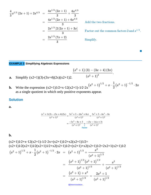
EXAMPLE 1 Forming the Sum, Difference, Product, and Quotient of Two Functions
Let f and g be two functions defined as
f(x)=x−1 and g(x)=4−x
Find the following functions and determine their domain:
a. (f+g)(x)
b. (f−g)(x)
c. (f⋅g)(x)
d. fg(x)
Solution The domain of f is {x|x≥1}, and the domain of g is {x|x≤4}.
a. (f+g)(x)=f(x)+g(x)=x−1+4−x. The
domain of (f+g)(x) is the closed interval [1,4].
b. (f−g)(x)=f(x)−g(x)=x−1−4−x. The
domain of (f−g)(x) is the closed interval [1,4].
c. (f⋅g)(x)=f(x)⋅g(x)=(x−1)(4−x)=−x2+5x−4.
The domain of (f⋅g)
(x) is the closed interval [1,4].
d. fg(x)=f(x)g(x)=x−14−x=−x2+5x−44−x.
The domain of fg(x) is the
half-open interval [1,4). ▪
NOW WORK Problem 11.
2 Form a Composite Function
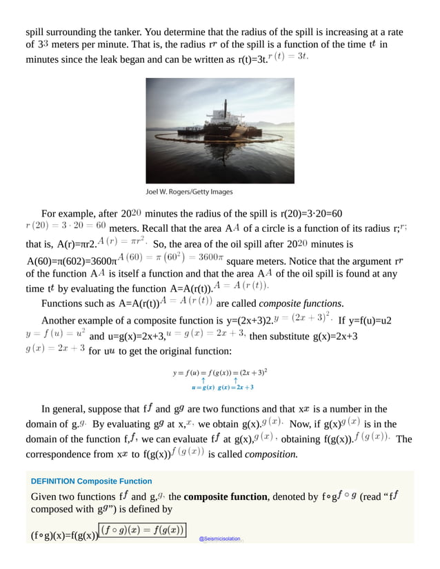
Suppose an oil tanker is leaking, and your job requires you to find the area of the circular oil
@Seismicisolation
@Seismicisolation

122. spill surrounding the tanker. You determine that the radius of the spill is increasing at a rate
of 3 meters per minute. That is, the radius r of the spill is a function of the time t in
minutes since the leak began and can be written as r(t)=3t.
For example, after 20 minutes the radius of the spill is r(20)=3⋅20=60
meters. Recall that the area A of a circle is a function of its radius r;
that is, A(r)=πr2. So, the area of the oil spill after 20 minutes is
A(60)=π(602)=3600π square meters. Notice that the argument r
of the function A is itself a function and that the area A of the oil spill is found at any
time t by evaluating the function A=A(r(t)).
Functions such as A=A(r(t)) are called composite functions.
Another example of a composite function is y=(2x+3)2. If y=f(u)=u2
and u=g(x)=2x+3, then substitute g(x)=2x+3
for u to get the original function:
y
equals
f
of
u
equals
f
open
parenthesis
g
In general, suppose that f and g are two functions and that x is a number in the
domain of g. By evaluating g at x, we obtain g(x). Now, if g(x) is in the
domain of the function f, we can evaluate f at g(x), obtaining f(g(x)). The
correspondence from x to f(g(x)) is called composition.
DEFINITION Composite Function
Given two functions f and g, the composite function, denoted by f∘g (read “f
composed with g ”) is defined by
(f∘g)(x)=f(g(x)) @Seismicisolation
@Seismicisolation

123. The domain of f∘g is the set of all numbers x in the domain of g for which g(x)
is in the domain of f.
Figure 42 illustrates the definition. Only those numbers x in the domain of g for which
g(x) is in the domain of f are in the domain of f∘g. As a result, the domain of
f∘g is a subset of the domain of g, and the range of f∘g is a subset of the range
of f.
Figure 42
EXAMPLE 2 Evaluating a Composite Function
Suppose that f(x)=1x+2 and g(x)=4x−1.
a. (f∘g)(0)=f(g(0))=f(−4)=1−4+2=−12g(x)=4x−1;g(0)=−4
b.
Open
parenthesis
g
o
f
c. (f∘f)(1)=f(f(1))=f13=113+2=173=37
@Seismicisolation
@Seismicisolation

124. d.
Open
parenthesis
g
o
g
close
parenthesis
of
negative
3
equals
g
open
parenthesis
g
of
negative
3
close
parenthesis
equals
g
of
negative
1
equals
4
over
negative
minus
1
equals
negative
2.
An
arrow
pointing
▪
NOTE The “inside” function g, in f(g(x)), is evaluated first.
NOW WORK Problem 15.
EXAMPLE 3 Finding the Domain of a Composite Function
Suppose that f(x)=1x+2 and g(x)=4x−1. Find f∘g and its
domain.
Solution
(f∘g)(x)=f(g(x))=1g(x)+2=14x−1+2=x−14+2(x−1)=x−12x+2
To find the domain of f∘g, first note that the domain of g is {x|x≠1},
so we exclude 1 from the domain of f∘g. Next note that the domain of f is {x|x≠−2},
which means g(x) cannot equal −2. To determine what additional
values of x to exclude, we solve the equation g(x)=−2:
4x−1=−2g(x)=−24=−2(x−1)4=−2x+22x=−2x=−1
We also exclude −1 from the domain of f∘g.
The domain of f∘g is {x|x≠−1, x≠1}. ▪
We could also find the domain of f∘g by first finding the domain of g: {x|x≠1}.
So, exclude 1 from the domain of f∘g. From (f∘g)(x)=x−12x+2=x
@Seismicisolation
@Seismicisolation

125. −12(x+1), notice that x≠−1, so we exclude −1
from the domain of f∘g. Therefore, the domain of f∘g is {x|x≠−1, x≠1}.
NOW WORK Problem 23.
In general, the composition of two functions f and g is not commutative. That is, f∘g
almost never equals g∘f. For example, in Example 3,
(g∘f)(x)=g(f(x))=4f(x)−1=41x+2−1=4(x+2)1−(x+2)=−4(x+2)x+1
Functions f and g for which f∘g=g∘f will be discussed in the next section.
Some techniques in calculus require us to “decompose” a composite function. For
example, the function H(x)=x+1 is the composition f∘g of the functions
f(x)=x and g(x)=x+1.
EXAMPLE 4 Decomposing a Composite Function
Find functions f and g so that f∘g=F when:
a. F(x)=1x+1
b. F(x)=(x3−4x−1)100
c. F(t)=2−t
Solution a. If we let f(x)=1x and g(x)=x+1, then
(f∘g)(x)=f(g(x))=1g(x)=1x+1=F(x)
b. If we let f(x)=x100 and g(x)=x3−4x−1, then
(f∘g)(x)=f(g(x))=f(x3−4x−1)=(x3−4x−1)100=F(x)
c. If we let f(t)=t and g(t)=2−t, then
@Seismicisolation
@Seismicisolation

126. (f∘g)(t)=f(g(t))=f(2−t)=2−t=F(t)
▪
Although the functions f and g chosen in Example 4 are not unique, there is usually a
“natural” selection for f and g that first comes to mind. When decomposing a composite
function, the “natural” selection for g is often an expression inside parentheses, in a
denominator, or under a radical.
NOW WORK Problem 27.
3 Transform the Graph of a Function with Vertical and Horizontal Shifts
At times we need to graph a function that is very similar to a function with a known graph.
Often techniques, called transformations, can be used to draw the new graph.
First we consider translations. Translations shift the graph from one position to another
without changing its shape, size, or direction.
For example, let f be a function with a known graph, say, f(x)=x2. If k is a
positive number, then adding k to f adds k to each y -coordinate, causing the graph of f
to shift vertically up k units. On the other hand, subtracting k from f subtracts k
from each y -coordinate, causing the graph of f to shift vertically down k units. See
Figure 43.
Figure 43
First
diagram
shows
a
parabolic
graph
So, adding (or subtracting) a positive constant to a function shifts the graph of the
original function vertically up (or down). Now we investigate how to shift the graph of a
function right or left.
Again, let f be a function with a known graph, say, f(x)=x2, and let h be a
positive number. To shift the graph to the right h units, subtract h from the argument of f.
In other words, replace the argument x of a function f by x−h, h>0. The
@Seismicisolation
@Seismicisolation

127. graph of the new function y=f(x−h) is the graph of f shifted horizontally
right h units. On the other hand, if we replace the argument x of a function f by
x+h, h>0, the graph of the new function y=f(x+h) is the graph of f
shifted horizontally left h units. See Figure 44.
Figure 44
First
diagram
shows
a
parabolic
graph
passing
through
origin
depicting
the
function
f
of
x
equals
x
square,
second
diagram
shows
a
parabolic
The graph of a function f can be moved anywhere in the plane by combining vertical
and horizontal shifts.
EXAMPLE 5 Combining Vertical and Horizontal Shifts
Use transformations to graph the function f(x)=(x+3)2−5.
Solution Graph f in steps:
Observe that f is basically a square function, so begin by graphing y=x2 in
Figure 45(a).
Replace the argument x with x+3 to obtain y=(x+3)2. This shifts
the graph of f horizontally to the left 3 units, as shown in Figure 45(b).
Finally, subtract 5 from each y -coordinate, which shifts the graph in Figure 45(b)
vertically down 5 units and results in the graph of f(x)=(x+3)2−5
shown in Figure 45(c).
@Seismicisolation
@Seismicisolation

128. Figure 45
First
diagram
shows
a
graph
depicting
the
function
y
equals
x
squared
which
passes
through
the
points
(minus
1,
1),
(0,
0)
and
(1,
1).
Second
diagram
▪
Notice the points plotted in Figure 45. Using key points can be helpful in keeping track of
the transformation that has taken place.
NOW WORK Problem 39.
4 Transform the Graph of a Function with Compressions and Stretches
When a function f is multiplied by a positive number a, the graph of the new function
y=af(x) is obtained by multiplying each y -coordinate on the graph of f by a.
The new graph is a vertically compressed version of the graph of f if 0<a<1 and
is a vertically stretched version of the graph of f if a>1. Compressions and stretches
change the proportions of a graph.
For example, the graph of f(x)=x2 is shown in Figure 46(a). Multiplying f by
a=12 produces a new function y=12 f(x)=12 x2, which vertically
compresses the graph of f by a factor of 12, as shown in Figure 46(b). On the other
hand, if a=3, then multiplying f by 3 produces a new function y=3f(x)=3x2,
and the graph of f is vertically stretched by a factor of 3, as shown in
Figure 46(c).
@Seismicisolation
@Seismicisolation

129. Figure 46
First
graph
depicts
the
function
f
of
x
equals
x
squared
and
passes
through
the
points
(minus
2,
4),
(0,
0)
and
(2,
4).
Second
graph
depicts
If the argument x of a function f is multiplied by a positive number a, the graph of
the new function y=f(ax) is a horizontal compression of the graph of f when
a>1 and a horizontal stretch of the graph of f when 0<a<1.
For example, the graph of y=f(2x)=(2x)2=4x2 is a horizontal
compression of the graph of f(x)=x2. See Figure 47(a) and 47(b). On the other
hand, if a=13, then the graph of y=13 x2=19 x2 is a horizontal
stretch of the graph of f(x)=x2. See Figure 47(c).
Figure 47
First
graph
depicts
the
5 Transform the Graph of a Function by Reflecting It About the x -axis or the y
-axis
The third type of transformation, reflection about the x - or y -axis, changes the orientation
@Seismicisolation
@Seismicisolation

130. of the graph of the function f but keeps the shape and the size of the graph intact.
When a function f is multiplied by −1, the graph of the new function y=−f(x)
is the reflection about the x -axis of the graph of f. For example, if f(x)=x,
then the graph of the new function y=−f(x)=−x is the
reflection of the graph of f about the x -axis. See Figure 48(a) and 48(b).
Figure 48
First
diagram
shows
a
curve
at
first
quadrant
depicting
the
function
f
of
x
equals
square
root
of
x
which
passes
through
the
If the argument x of a function f is multiplied by −1, then the graph of the new
function y=f(−x) is the reflection about the y -axis of the graph of f. For
example, if f(x)=x, then the graph of the new function y=f(−x)=−x
is the reflection of the graph of f about the y -axis. See Figure 48(a)
and 48(c). Notice in this example that the domain of y=−x is all real numbers for
which −x≥0, or equivalently, x≤0.
EXAMPLE 6 Combining Transformations
Use transformations to graph the function f(x)=1−x+2.
Solution We graph f in steps:
Observe that f is basically a square root function, so we begin by graphing y=x.
See Figure 49(a).
Now replace the argument x with x+1 to obtain y=x+1, which shifts
the graph of y=x horizontally to the left 1 unit, as shown in Figure 49(b).
Then replace x with −x to obtain y=−x+1=1−x, which
reflects the graph about the y -axis. See Figure 49(c).
Finally, add 2 to each y -coordinate, which shifts the graph vertically up 2 units and
results in the graph of f(x)=1−x+2 shown in Figure 49(d).
@Seismicisolation
@Seismicisolation

131. Figure 49
First
graph
depicts
the
function
y
equals
squared
square
root
of
x
and
passes
through
the
points
(0,
0),
(1,
1)
and
(4,
2).
Second
graph
depicts
the
function
y
equals
NOW WORK Problem 43.
P.3 Assess Your Understanding
Concepts and Vocabulary
1. If the domain of a function f is {x|0≤x≤7} and the domain of a function
g is {x|−2≤x≤5}, then the domain of the sum function f+g
is__________.
2. True or False If f and g are functions, then the domain of fg consists of all
numbers x that are in the domains of both f and g.
3. True or False The domain of f⋅g consists of the numbers x that are in the
domains of both f and g.
4. True or False The domain of the composite function f∘g is the same as the
domain of g(x).
5. True or False The graph of y=−f(x) is the reflection of the graph of y=f(x)
about the x -axis.
6. True or False To obtain the graph of y=f(x+2)−3, shift the graph of
y=f(x) horizontally to the right 2 units and vertically down 3 units.
7. True or False Suppose the x -intercepts of the graph of the function f are −3 and
2. Then the x -intercepts of the graph of the function y=2f(x) are −3
and 2.
8. Suppose that the graph of a function f is known. Then the graph of the function y=f(x
−2) can be obtained by a(n)__________ shift of the graph of f to the
@Seismicisolation
@Seismicisolation

132. __________ a distance of 2 units.
9. Suppose that the graph of a function f is known. Then the graph of the function
y=f(−x) can be obtained by a reflection about the__________ -axis of the
graph of f.
10. Suppose the x -intercepts of the graph of the function f are −2, 1, and 5. The
x -intercepts of y=f(x+3) are__________,__________, and__________.
Practice Problems
In Problems 11–14, the functions f and g are given. Find each of the following functions
and determine their domain:
a. (f+g)(x)
b. (f−g)(x)
c. (f⋅g)(x)
d. fg(x)
11. f(x)=3x+4 and g(x)=2x−3
12. f(x)=1+1x and g(x)=1x
13. f(x)=x+1 and g(x)=2x
14. f(x)=|x |and g(x)=x
In Problems 15 and 16, for each of the functions f and g, find:
a. (f∘g)(4)
b. (g∘f)(2)
c. (f∘f)(1)
d. (g∘g)(0)
15. f(x)=2x and g(x)=3x2+1
16. f(x)=3x+1 and g(x)=x
@Seismicisolation
@Seismicisolation

133. In Problems 17 and 18, evaluate each expression using the values given in the table.
17.
x −3 −2 −1 0 1 2 3
f(x) −7 −5 −3 −1 3 5 7
g(x) 8 3 0 −1 0 3 8
a. (f∘g)(1)
b. (f∘g)(−1)
c. (g∘f)(−1)
d. (g∘f)(1)
e. (g∘g)(−2)
f. (f∘f)(−1)
18.
x −3 −2 −1 0 1 2 3
f(x) 11 9 7 5 3 1 −1
g(x) −8 −3 0 1 0 −3 −8
a. (f∘g)(1)
b. (f∘g)(2)
c. (g∘f)(2)
d. (g∘f)(3)
e. (g∘g)(1)
f. (f∘f)(3)
In Problems 19 and 20, evaluate each composite function using the graphs of
y=f(x) and y=g(x) shown in the figure below.
19. a. (g∘f)(−1)
b. (g∘f)(6)
c. (f∘g)(6)
d. (f∘g)(4)
20. a. (g∘f)(1)
b. (g∘f)(5)
c. (f∘g)(7)
d. (f∘g)(2)
@Seismicisolation
@Seismicisolation

134. The
up
and
down
graph
begins
at
(minus
1,
3)
on
the
second
quadrant
and
ends
at
(7,
5)
on
the
first
quadrant.
The
V-
shaped
graph
linearly
decreases
In Problems 21–26, for the given functions f and g, find:
a. f∘g
b. g∘f
c. f∘f
d. g∘g
State the domain of each composite function.
21. f(x)=3x+1 and g(x)=8x
22. f(x)=−x and g(x)=2x−4
23. f(x)=x2+1 and g(x)=x−1
24. f(x)=2x+3 and g(x)=x
25. f(x)=xx−1 and g(x)=2x
26. f(x)=1x+3 and g(x)=−2x
In Problems 27–32, find functions f and g so that f∘g=F.
27. F(x)=(2x+3)4
28. F(x)=(1+x2)3
29. F(x)=x2+1
@Seismicisolation
@Seismicisolation

135. 30. F(x)=1−x2
31. F(x)=|2x+1|
32. F(x)=|2x2+3|
In Problems 33–46, graph each function using the graphing techniques of shifting,
compressing, stretching, and/or reflecting. Begin with the graph of a basic function and show
all stages.
33. f(x)=x3+2
34. g(x)=x3−1
35. h(x)=x−2
36. f(x)=x+1
37. g(x)=4x
38. f(x)=12x
39. f(x)=(x−1)3+2
40. g(x)=3(x−2)2+1
41. h(x)=12x
42. f(x)=4x+2
43. G(x)=2|1−x|
44. g(x)=−(x+1)3−1
45. g(x)=−4x−1
46. f(x)=42−x
In Problems 47 and 48, the graph of a function f is illustrated. Use the graph of f as the first
step in graphing each of the following functions:
a. F(x)=f(x)+3
b. G(x)=f(x+2)
@Seismicisolation
@Seismicisolation

136. c. P(x)=−f(x)
d. H(x)=f(x+1)−2
e. Q(x)=12 f(x)
f. g(x)=f(−x)
g. h(x)=f(2x)
47.
48.
49. Period of a Pendulum The period T (in seconds) of a simple pendulum is a function
of its length l (in meters) defined by the equation
T=T(l)=2πlg
where g≈9.8 meters/second2 is the acceleration due to gravity.
a. Use technology to graph the function T=T(l).
b. Now graph the functions T=T(l+1), T=T(l+2), and
@Seismicisolation
@Seismicisolation

137. T=T(l+3).
c. Discuss how adding to the length l changes the period T.
d. Now graph the functions T=T(2l), T=T(3l), and T=T(4l).
e. Discuss how multiplying the length l by 2, 3, and 4 changes the period T.
50. Suppose (1,3) is a point on the graph of y=g(x).
a. What point is on the graph of y=g(x+3)−5?
b. What point is on the graph of y=−2g(x−2)+1?
c. What point is on the graph of y=g(2x+3)?
1. = NOW WORK problem
= Graphing technology recommended
= Computer Algebra System recommended
@Seismicisolation
@Seismicisolation

138. P.4 Inverse Functions
OBJECTIVES When you finish this section, you should be able to:
1 Determine whether a function is one-to-one
2 Determine the inverse of a function defined by a set of ordered pairs
3 Obtain the graph of the inverse function from the graph of a one-to-one
function
4 Find the inverse of a one-to-one function defined by an equation
1 Determine Whether a Function Is One-to-One
By definition, for a function y=f(x), if x is in the domain of f, then x has one,
and only one, image y in the range. If a function f also has the property that no y in the
range of f is the image of more than one x in the domain, then the function is called a
one-to-one function.
DEFINITION One-to-One Function
A function f is a one-to-one function if any two different inputs in the domain correspond
to two different outputs in the range. That is, if x1≠x2, then f(x1)≠f(x2).
IN WORDS A function is not one-to-one if there are two different inputs in the domain corresponding to the
same output.
Figure 50 illustrates the distinction among one-to-one functions, functions that are not
one-to-one, and relations that are not functions.
@Seismicisolation
@Seismicisolation

139. Figure 50
In
one-
to-
one
function,
x
subscript
1
from
domain
is
connected
to
y
subscript
1
in
range,
x
subscript
2
from
domain
is
connected
to
y
If the graph of a function f is known, there is a simple test called the Horizontal-line
Test, to determine whether f is a one-to-one function.
THEOREM Horizontal-line Test
The graph of a function in the xy -plane is the graph of a one-to-one function if and only
if every horizontal line intersects the graph in at most one point.
EXAMPLE 1 Determining Whether a Function Is One-to-One
Determine whether each of these functions is one-to-one:
a. f(x)=x2
b. g(x)=x3
Solution a. Figure 51 illustrates the Horizontal-line Test for the graph of f(x)=x2.
The horizontal line y=1 intersects the graph of f twice, at (1,1) and
at (−1,1), so f is not one-to-one.
@Seismicisolation
@Seismicisolation

140. Figure 51
b. Figure 52 illustrates the Horizontal-line Test for the graph of g(x)=x3. Because
every horizontal line intersects the graph of g exactly once, it follows that g is one-to-one.
Figure 52
▪
NOW WORK Problem 9.
Notice that the one-to-one function g(x)=x3 also is an increasing function on
its domain. Because an increasing (or decreasing) function will always have different y -
@Seismicisolation
@Seismicisolation

141. values for different x -values, a function that is increasing (or decreasing) on an interval is
also a one-to-one function on that interval.
THEOREM One-to-One Function
A function that is increasing on an interval I is a one-to-one function on I.
A function that is decreasing on an interval I is a one-to-one function on I.
Suppose that f is a one-to-one function. Then to each x in the domain of f, there is
exactly one image y in the range (because f is a function); and to each y in the range of
f, there is exactly one x in the domain (because f is one-to-one). The correspondence
from the range of f back to the domain of f is also a function, called the inverse function
of f. The symbol f−1 is used to denote the inverse of f.
DEFINITION Inverse Function
Let f be a one-to-one function. The inverse of f, denoted by f−1, is the function
defined on the range of f for which
x=f−1(y)if and only ify=f(x)
NOTE f−1 is not the reciprocal function. That is, f−1(x)≠1f(x). The reciprocal function
1f(x) is written [f(x)]−1.
We will discuss how to find inverses for three representations of functions: (1) sets of
ordered pairs, (2) graphs, and (3) equations. We begin with finding the inverse of a function
represented by a set of ordered pairs.
2 Determine the Inverse of a Function Defined by a Set of Ordered Pairs
If the function f is a set of ordered pairs (x,y), then the inverse of f, denoted f−1,
is the set of ordered pairs (y,x).
EXAMPLE 2 Finding the Inverse of a Function Defined by a Set of Ordered Pairs
Find the inverse of the one-to-one function:
@Seismicisolation
@Seismicisolation

142. {(−3,−5),(−1,1),(0,2),(1,3)}
State the domain and the range of the function and its inverse.
Solution The inverse of the function is found by interchanging the entries in each ordered
pair. The inverse is
{(−5,−3),(1,−1),(2,0),(3,1)}
The domain of the function is {−3,−1,0,1} ; the range of the function is
{−5,1,2,3}. The domain of the inverse function is {−5,1,2,3} ; the
range of the inverse function is {−3,−1,0,1}. ▪
Figure 53 shows the one-to-one function (in blue) and its inverse (in red).
Figure 53
The
points
(minus
1,
1),
(0,
2),
(1,
3)
NOW WORK Problem 19.
Remember, if f is a one-to-one function, it has an inverse f−1. See Figure 54.
Based on the results of Example 2 and Figure 53, two properties of a one-to-one function f
and its inverse function f−1 become apparent:
Domain of f=Range of f−1Range of f=Domain of f−1
@Seismicisolation
@Seismicisolation

143. Figure 54
The next theorem provides a means for verifying that two functions are inverses of one
another.
THEOREM
Given a one-to-one function f and its inverse function f−1, then
(f−1∘f)(x)=f−1(f (x))=xwhere x is in the domain of f
(f∘f−1)(x)=f (f−1(x))=xwhere x is in the domain of f−1
EXAMPLE 3 Verifying Inverse Functions
Verify that the inverse of f(x)=1x−1 is f−1(x)=1x+1. For
what values of x is f−1(f(x))=x? For what values of x is f(f−1(x))=x?
Solution The domain of f is {x|x≠1} and the domain of f−1 is {x|x≠0}.
Now
f−1(f(x))=f−11x−1=11x−1+1=x−1+1=xprovided x≠1f(f
−1(x))=f1x+1=11x+1−1=11x=xprovided x≠0
@Seismicisolation
@Seismicisolation

144. ▪
NOW WORK Problem 15.
3 Obtain the Graph of the Inverse Function from the Graph of a One-to-One
Function
Suppose (a,b) is a point on the graph of a one-to-one function f defined by y=f(x).
Then b=f(a). This means that a=f−1(b), so (b,a) is a
point on the graph of the inverse function f−1. Figure 55 shows the relationship between
the point (a,b) on the graph of f and the point (b,a) on the graph of f−1.
The line segment containing (a,b) and (b,a) is perpendicular to the line y=x
and is bisected by the line y=x. (Do you see why?) The point (b,a) on the graph
of f−1 is the reflection about the line y=x of the point (a,b) on the graph of f.
Figure 55
THEOREM Symmetry of Inverse Functions
@Seismicisolation
@Seismicisolation

145. The graph of a one-to-one function f and the graph of its inverse function f−1 are
symmetric with respect to the line y=x.
We can use this result to find the graph of f−1 given the graph of f. If we know the
graph of f, then the graph of f−1 is obtained by reflecting the graph of f about the line
y=x. See Figure 56.
Figure 56
EXAMPLE 4 Graphing the Inverse Function from the Graph of a Function
The graph in Figure 57 is that of a one-to-one function y=f(x). Draw the graph of
its inverse function.
@Seismicisolation
@Seismicisolation

146. Figure 57
Solution Since the points (−2,−1), (−1,0), and (2,1) are on the
graph of f, the points (−1,−2), (0,−1), and (1,2) are on the graph of
f−1. Using the points and the fact that the graph of f−1 is the reflection about the
line y=x of the graph of f, draw the graph of f−1, as shown in Figure 58. ▪
Figure 58
The
line
f
of
NOW WORK Problem 27.
4 Find the Inverse of a One-to-One Function Defined by an Equation
@Seismicisolation
@Seismicisolation

147. Since the graphs of a one-to-one function f and its inverse function f−1 are symmetric
with respect to the line y=x, the inverse function f−1 can be obtained by
interchanging the roles of x and y in f. If f is defined by the equation
y=f(x)
then f−1 is defined by the equation
x=f(y)Interchange x and y.
The equation x=f(y) defines f−1 implicitly. If the implicit equation can be
solved for y, we will have the explicit form of f−1, that is,
y=f−1(x)
Steps for Finding the Inverse of a One-to-One Function
Step 1 Write f in the form y=f(x).
Step 2 Interchange the variables x and y to obtain x=f(y). This equation
defines the inverse function f−1 implicitly.
Step 3 If possible, solve the implicit equation for y in terms of x to obtain the explicit
form of f−1: y=f−1(x).
Step 4 Check the result by showing that f−1(f (x))=x and f (f−1(x))=x.
EXAMPLE 5 Finding the Inverse Function
The function f(x)=2x3−1 is one-to-one. Find its inverse.
Solution We follow the steps given above.
Step 1 Write f as y=2x3−1.
Step 2 Interchange the variables x and y.
x=2y3−1
This equation defines f−1 implicitly.
Step 3 Solve the implicit form of the inverse function for y.
@Seismicisolation
@Seismicisolation

148. x+1=2y3y3=x+12y=x+123=f−1(x)
Step 4 Check the result.
f−1(f(x))=f−1(2x3−1)=(2x3−1)+123=2x323=x33=xf(f
−1(x))=fx+123=2x+1233−1=2x+12−1=x+1−1=x
▪
See Figure 59 for the graphs of f and f−1.
Figure 59
The
curves
depict
NOW WORK Problem 31.
If a function f is not one-to-one, it has no inverse function. But sometimes we can
@Seismicisolation
@Seismicisolation

149. restrict the domain of such a function so that it is a one-to-one function. Then on the
restricted domain the new function has an inverse function.
EXAMPLE 6 Finding the Inverse of a Domain-Restricted Function
Find the inverse of f(x)=x2 if x≥0.
Solution The function f(x)=x2 is not one-to-one (see Example 1(a)). However, by
restricting the domain of f to x≥0, the new function f is one-to-one, so f−1
exists. To find f−1, follow the steps.
Step 1 y=x2, where x≥0.
Step 2 Interchange the variables x and y: x=y2, where y≥0. This is the
inverse function written implicitly.
Step 3 Solve for y: y=x=f−1(x). (Since y≥0, only the principal
square root is obtained.)
Step 4 Check that f−1(x)=x is the inverse function of f.
f−1(f(x))=f(x)=x2=|x|=xwhere x≥0f(f−1(x))=[f−1(x)]2=[x]2=xwhere x≥0
▪
The graphs of f(x)=x2, x≥0, and f−1(x)=x are shown in
Figure 60.
@Seismicisolation
@Seismicisolation

150. Figure 60
The
curves
depict
the
one-
to-
one
function
f
of
x
equals
x
squared
for
x
greater
than
or
equal
to
0
and
NEED TO REVIEW? Principal roots are discussed in Appendix A.1, p. A-9.
NOW WORK Problem 37.
P.4 Assess Your Understanding
Concepts and Vocabulary
1. True or False If every vertical line intersects the graph of a function f at no more than
one point, f is a one-to-one function.
2. If the domain of a one-to-one function f is [4,∞), the range of its inverse
function f−1 is __________.
3. True or False If f and g are inverse functions, the domain of f is the same as the
domain of g.
4. True or False If f and g are inverse functions, their graphs are symmetric with
respect to the line y=x.
5. True or False If f and g are inverse functions, then (f∘g)(x)=f(x)⋅g(x).
@Seismicisolation
@Seismicisolation

151. 6. True or False If a function f is one-to-one, then f(f−1(x))=x, where x
is in the domain of f.
7. Given a collection of points (x,y), explain how you would determine if it
represents a one-to-one function y=f(x).
8. Given the graph of a one-to-one function y=f (x), explain how you would
graph the inverse function f−1.
Practice Problems
In Problems 9–14, the graph of a function f is given. Use the Horizontal-line Test to
determine whether f is one-to one.
9.
10.
@Seismicisolation
@Seismicisolation

152. 11.
12.
13.
@Seismicisolation
@Seismicisolation

153. 14.
In Problems 15–18, verify that the functions f and g are inverses of each other by showing
that (f∘g)(x)=x and (g∘f)(x)=x .
15. f(x)=3x+4 ; g(x)=13 (x−4)
16. f(x)=x3−8 ; g(x)=x+83
17. f(x)=1x ; g(x)=1x
18. f(x)=2x+3x+4 ; g(x)=4x−32−x
In Problems 19–22, (a) determine whether the function is one-to-one. If it is one-to-one, (b)
find the inverse of each function. (c) State the domain and the range of the function and its
inverse.
19. {(−3,5),(−2,9),(−1,2),(0,11),(1,−5)}
20. {(−2,2),(−1,6),(0,8),(1,−3),(2,8)}
21. {(−2,1),(−3,2),(−10,0),(1,9),(2,1)}
22. {(−2,−8),(−1,−1),(0,0),(1,1),(2,8)}
In Problems 23–28, the graph of a one-to-one function f is given. Draw the graph of the
inverse function. For convenience, the graph of y=x is also given.
23.
@Seismicisolation
@Seismicisolation

154. 24.
25.
26.
@Seismicisolation
@Seismicisolation

155. 27.
28.
In Problems 29–38, the function f is one-to-one.
@Seismicisolation
@Seismicisolation

156. a. Find its inverse and check the result.
b. Find the domain and the range of f and the domain and the range of f−1 .
29. f(x)=4x+2
30. f(x)=1−3x
31. f(x)=x+103
32. f(x)=2x3+4
33. f(x)=1x−2
34. f(x)=2x3x−1
35. f(x)=2x+3x+2
36. f(x)=−3x−4x−2
37. f(x)=x2+4, x≥0
38. f(x)=(x−2)2+4, x≤2
1. = NOW WORK problem
= Graphing technology recommended
= Computer Algebra System recommended
@Seismicisolation
@Seismicisolation

157. P.5 Exponential and Logarithmic Functions
OBJECTIVES When you finish this section, you should be able to:
1 Analyze an exponential function
2 Define the number e
3 Analyze a logarithmic function
4 Solve exponential equations and logarithmic equations
We begin our study of transcendental functions with the exponential and logarithmic
functions. In Sections P.6 and P.7, we investigate the trigonometric functions and their
inverse functions.
1 Analyze an Exponential Function
The expression ar, where a>0 is a fixed real number and r=mn is a rational
number, in lowest terms with n≥2, is defined as
ar=am⁄n=(a1⁄n)m=(an)m
So, a function f(x)=ax can be defined so that its domain is the set of rational
numbers. Our aim is to expand the domain of f to include both rational and irrational
numbers, that is, to include all real numbers.
CAUTION Be careful to distinguish an exponential function f(x)=ax, where a>0 and a≠1,
from a power function g(x)=xa, where a is a real number. In f(x)=ax the
independent variable x is the exponent; in g(x)=xa the independent variable x is the base.
Every irrational number x can be approximated by a rational number r formed by
truncating (removing) all but a finite number of digits from x. For example, for x=π,
we could use the rational numbers r=3.14 or r=3.14159, and so
on. The closer r is to π, the better approximation ar is to aπ. In general, we can
make ar as close as we please to ax by choosing r sufficiently close to x. Using this
argument, we can define an exponential function f(x)=ax, where x includes all
the rational numbers and all the irrational numbers.
DEFINITION Exponential Function
@Seismicisolation
@Seismicisolation

158. An exponential function is a function that can be expressed in the form
f(x)=ax
where a is a positive real number and a≠1. The domain of f is the set of all real
numbers.
NOTE The base a=1 is excluded from the definition of an exponential function because f(x)=1x=1
(a constant function). Bases that are negative are excluded because a1⁄n, where a<0
and n is an even integer, is not defined.
Examples of exponential functions are f(x)=2x, g(x)=23x, and h(x)=πx.
Consider the exponential function f(x)=2x. The domain of f is all real
numbers; the range of f is the interval 0,∞. Some points on the graph of f are
listed in Table 5. Since 2x>0 for all x, the graph of f lies above the x -axis and
has no x -intercept. The y -intercept is 1. Using this information, plot some points from
Table 5 and connect them with a smooth curve, as shown in Figure 61.
TABLE 5
x f(x)=2x (x,y)
−10 2−10≈0.00098 (−10,0.00098)
−3
2−3=18 −3,18
−2
2−2=14 −2,14
−1
2−1=12 −1,12
0 20=1 (0,1)
1 21=2 (1,2)
2 22=4 (2,4)
3 23=8 (3,8)
10 210=1024 (10,1024)
@Seismicisolation
@Seismicisolation

159. Figure 61 f(x)=2x
The graph of f(x)=2x is typical of all exponential functions of the form f(x)=ax
with a>1, a few of which are graphed in Figure 62.
Figure 62 f(x)=ax;a>1
Notice that every graph in Figure 62 lies above the x -axis, passes through the point
(0,1), and is increasing. Also notice that the graphs with larger bases are steeper when
x>0, but when x<0, the graphs with larger bases are closer to the x -axis.
All functions of the type f(x)=ax, a>1, have the following properties:
@Seismicisolation
@Seismicisolation

160. Properties of an Exponential Function f(x)=ax,a>1
The domain is the set of all real numbers; the range is the set of positive real numbers.
There are no x -intercepts; the y -intercept is 1.
The exponential function f is increasing on the interval (−∞,∞).
The graph of f contains the points −1,1a, (0,1), and (1,a).
f(x+1)f(x)=a
Because f(x)=ax is a function, if u=v, then au=av.
Because f(x)=ax is a one-to-one function, if au=av, then u=v.
THEOREM Laws of Exponents
If u, v, a, and b are real numbers with a>0 and b>0, then
au⋅av=au+vauav=au−v(au)v=auv(ab)u=au⋅bu(ab)u=aubu
NEED TO REVIEW? The Laws of Exponents are discussed in Appendix A.1, pp. A-8 to A-9.
For example, we can use the Laws of Exponents to show the following property of an
exponential function:
f(x+1)f(x)=ax+1ax=a(x+1)−x=a1=a
EXAMPLE 1 Graphing an Exponential Function
Graph the exponential function g(x)=12x.
Solution We begin by writing 12 as 2−1. Then
@Seismicisolation
@Seismicisolation

161. g(x)=12x=(2−1)x=2−x
Now use the graph of f(x)=2x shown in Figure 61 and reflect the graph about
the y -axis to obtain the graph of g(x)=2−x. See Figure 63.
Figure 63
▪
NOW WORK Problem 19.
The graph of g(x)=12x in Figure 63 is typical of all exponential functions
that have a base between 0 and 1. Figure 64 illustrates the graphs of several more exponential
functions whose bases are between 0 and 1. Notice that the graphs with smaller bases are
steeper when x<0, but when x>0, these graphs are closer to the x -axis.
@Seismicisolation
@Seismicisolation

162. Figure 64 f(x)=ax,0<a<1
Properties of an Exponential Function f(x)=ax,0<a<1
The domain is the set of all real numbers; the range is the set of positive real numbers.
There are no x -intercepts; the y -intercept is 1.
The exponential function f is decreasing on the interval (−∞,∞).
The graph of f contains the points (−1,1a), (0,1), and (1,a).
f(x+1)f(x)=a
If u=v, then au=av.
If au=av, then u=v.
EXAMPLE 2 Graphing an Exponential Function Using Transformations
Graph f(x)=3−x−2 and determine the domain and range of f.
Solution We begin with the graph of y=3x. Figure 65 shows the steps.
@Seismicisolation
@Seismicisolation

163. Figure 65
In
the
first
step,
an
exponentially
rising
curve
3
to
the
power
x
is
drawn.
In
the
second
step,
x
is
replaced
with
minus
x,
and
then
the
curve
reflects
about
The domain of f is all real numbers; the range of f is the interval (−2,∞ ). ▪
NOW WORK Problem 27.
2 Define the Number e
In earlier courses you learned about an irrational number, called e. The number e is
important because it appears in many applications and because it has properties that simplify
computations in calculus.
To define e, consider the graphs of the functions y=2x and y=3x in
Figure 66(a), where we have carefully drawn lines that just touch each graph at the point
(0,1). (These lines are tangent lines, which we discuss in Chapter 1.) Notice that the
slope of the tangent line to y=3x is greater than 1 (approximately 1.10 ) and that
the slope of the tangent line to the graph of y=2x is less than 1 (approximately 0.69
). Between these graphs there is an exponential function y=ax, whose base is
between 2 and 3, and whose tangent line to the graph at the point (0,1) has a slope
of exactly 1, as shown in Figure 66(b). The base of this exponential function is the number e.
@Seismicisolation
@Seismicisolation

164. Figure 66
DEFINITION The number e
The number e is defined as the base of the exponential function whose tangent line to the
graph at the point 0,1 has slope 1. The function f(x)=ex occurs with such
frequency that it is usually referred to as the exponential function.
The number e is an irrational number, and in Chapter 3, we will show e≈2.71828.
ORIGINS The irrational number we call e was named to honor the Swiss mathematician Leonhard Euler
(1707–1783), who is considered one of the greatest mathematicians of all time. Euler was encouraged to study
mathematics by his father. Considered the most prolific mathematician who ever lived, he made major
@Seismicisolation
@Seismicisolation

165. contributions to many areas of mathematics. One of Euler’s greatest gifts was his ability to explain diffcult
mathematical concepts in simple language.
3 Analyze a Logarithmic Function
Recall that a one-to-one function y=f(x) has an inverse function that is defined
implicitly by the equation x=f(y). Since an exponential function y=f(x)=ax,
where a>0 and a≠1, is a one-to-one function, it has an inverse
function, called a logarithmic function, that is defined implicitly by the equation
x=aywhere a>0anda≠1
NEED TO REVIEW? Logarithms and their properties are discussed in Appendix A.1, pp. A-10 to A-11.
DEFINITION Logarithmic Function
The logarithmic function with base a, where a>0 and a≠1, is denoted by
y=logax and is defined by
y=logaxif and only ifx=ay
The domain of the logarithmic function y=logax is x>0.
IN WORDS A logarithm is an exponent. That is, if y=logax, then y is the exponent in x=ay.
In other words, if f(x)=ax, where a>0 and a≠1, its inverse
function is f−1(x)=logax.
If the base of a logarithmic function is the number e, then it is called the natural
logarithmic function, and it is given a special symbol, ln (from the Latin logarithmus
naturalis). That is,
y=ln xif and only ifx=ey
Since the exponential function y=ax, a>0,a≠1 and the logarithmic
function y=logax are inverse functions, the following properties hold:
loga(ax)=x for all real numbers x
alogax=x for all x>0
@Seismicisolation
@Seismicisolation

166. Because exponential functions and logarithmic functions are inverses of each other, the
graph of the logarithmic function y=logax, a>0 and a≠1, is the
reflection of the graph of the exponential function y=ax, about the line y=x, as
shown in Figure 67.
Figure 67
When
a
is
between
0
and
1,
both
curves
and
the
line
y
equal
to
x
intersect
at
a
point
Based on the graphs in Figure 67, we see that
loga1=0logaa=1a>0anda≠1
EXAMPLE 3 Graphing a Logarithmic Function
Graph:
a. f(x)=log2x
b. g(x)=log1⁄3x
c. F(x)=ln x
Solution a. To graph f(x)=log2x, graph y=2x and reflect it about the
line y=x. See Figure 68(a).
b. To graph g(x)=log1⁄3x, graph y=13x and reflect it about the
line y=x. See Figure 68(b).
c. To graph F(x)=ln x, graph y=ex and reflect it about the line y=x.
See Figure 68(c). @Seismicisolation
@Seismicisolation

167. Figure 68
The
reflection
of
logarithm
of
x
in
base
2
about
the
line
y
equal
to
x
gives
the
exponential
graph
2
raised
to
x.
The
reflection
of
logarithm
▪
NOW WORK Problem 39.
Since a logarithmic function is the inverse of an exponential function, it follows that
Domain of the logarithmic function=Range of the exponential function=(0,∞)
Range of the logarithmic function=Domain of the exponential function=(−∞,∞)
The domain of a logarithmic function is the set of positive real numbers, so the argument of a
logarithmic function must be greater than zero.
EXAMPLE 4 Finding the Domain of a Logarithmic Function
Find the domain of each function:
a. F(x)=log2(x+3)
b. g(x)=ln1+x1−x
c. h(x)=log1⁄2|x |
@Seismicisolation
@Seismicisolation

168. Solution a. The argument of a logarithm must be positive. So to find the domain of
F(x)=log2(x+3), we solve the inequality x+3>0. The domain
of F is {x|x>−3}.
NEED TO REVIEW? Solving inequalities is discussed in Appendix A.1, pp. A-5 to A-8.
b. Since ln1+x1−x requires 1+x1−x>0, we find the domain of g by
solving the inequality 1+x1−x>0. Since 1+x1−x is not defined for x=1,
and the solution to the equation 1+x1−x=0 is x=−1, we use −1
and 1 to separate the real number line into three intervals (−∞,−1), (−1,1),
and (1,∞). Then we choose a test number in each interval and evaluate the
rational expression 1+x1−x at these numbers to determine if the expression is positive
or negative. For example, we chose the numbers −2, 0, and 2 and found that
1+x1−x>0 on the interval (−1,1). See the table on the left. So the domain
of g(x)=ln1+x1−x is {x|−1<x<1}.
Interval Test Number
Sign of 1+x1−x
(−∞,−1) −2 Negative
(−1,1) 0 Positive
(1,∞) 2 Negative
c. log1⁄2|x | requires | x|>0. So the domain of h(x)=log1⁄2|x |
is {x|x≠0}. ▪
NOW WORK Problem 31.
Properties of a Logarithmic Function f(x)=logax, a>0 and a≠1
The domain of f is the set of all positive real numbers; the range is the set of all real
numbers.
@Seismicisolation
@Seismicisolation

169. The x -intercept of the graph of f is 1. There is no y -intercept.
A logarithmic function is decreasing on the interval (0,∞) if 0<a<1 and
increasing on the interval (0,∞) if a>1.
The graph of f contains the points (1,0), (a,1), and 1a,−1.
Because f(x)=logax is a function, if u=v, then logau=logav.
Because f(x)=logax is a one-to-one function, if logau=logav,
then u=v.
See Figure 69 on page 48 for typical graphs with base a, a>1; see Figure 70 for
graphs with base a, 0<a<1.
Figure 69 y=logax,a>1
@Seismicisolation
@Seismicisolation

170. Figure 70 y=logax,0<a<1
4 Solve Exponential Equations and Logarithmic Equations
Equations that involve terms of the form ax, a>0, a≠1, are referred to as
exponential equations. For example, the equation 52x+3=5x is an exponential
equation.
The one-to-one property of exponential functions
if au=avthen u=v
(1)
can be used to solve certain kinds of exponential equations.
IN WORDS In an exponential equation, if the bases are equal, then the exponents are equal.
EXAMPLE 5 Solving Exponential Equations
Solve each exponential equation:
a. 42x−1=8x+3
b. e−x2=(ex)2⋅1e3
Solution a. We begin by expressing both sides of the equation with the same base so that we
@Seismicisolation
@Seismicisolation

171. can use the one-to-one property (1).
42x−1=8x+3(22)2x−1=(23)x+34=22,8=2322(2x−1)=23(x+3)(ar)s=ars2(2x
−1)=3(x+3)If au=av,then u=v.4x−2=3x+9Simplify.x=11Solve.
The solution is 11.
b. We use the Laws of Exponents to obtain the base e on the right side.
(ex)2⋅1e3=e2x⋅e−3=e2x−3
As a result,
e−x2=e2x−3−x2=2x−3If au=av, then u=v.x2+2x−3=0(x+3)(x−1)=0x=−3orx=1
The solution set is {−3,1}. ▪
NOW WORK Problem 49.
To use the one-to-one property of exponential functions, each side of the equation must
be written with the same base. Since for many exponential equations it is not possible to
write each side with the same base, we need a different strategy to solve such equations.
EXAMPLE 6 Solving Exponential Equations
Solve the exponential equations:
a. 102x=50
b. 8⋅3x=5
@Seismicisolation
@Seismicisolation

172. RECALL Logarithms to the base 10 are called common logarithms and are written without a subscript.
That is, x=log10 y is written x=log y.
Solution a. Since 10 and 50 cannot be written with the same base, we write the
exponential equation as a logarithm.
102x=50if and only iflog 50=2x
Then x=log 502 is an exact solution of the equation. Using a calculator, an
approximate solution is x=log 502≈0.849.
b. It is impossible to write 8 and 5 as a power of 3, so we write the exponential equation
as a logarithm.
8⋅3x=53x=58x=log358
The Change-of-Base Formula can be used with a calculator to obtain an approximate
solution.
x=log358=ln 58ln3≈−0.428
NEED TO REVIEW? The Change-of-Base Formula, logau=logbulogba, a≠1, b≠1,
and u positive real numbers, is discussed in Appendix A.1, p. A-11.
▪
Alternatively, we could have solved each of the equations in Example 6 by taking the
natural logarithm (or the common logarithm) of each side. For example,
8⋅3x=5 3x=58 ln 3x=ln 58 If u=v, then logau=logav.x ln3=ln 58 loga ur=r logaux=ln 58ln3
@Seismicisolation
@Seismicisolation

173. NOW WORK Problem 51.
Equations that contain logarithms are called logarithmic equations. Care must be taken
when solving logarithmic equations algebraically. In the expression logay, remember
that a and y are positive and a≠1. Be sure to check each apparent solution in the
original equation and to discard any solutions that are extraneous.
Some logarithmic equations can be solved by changing the logarithmic equation to an
exponential equation using the fact that x=logay if and only if y=ax.
EXAMPLE 7 Solving Logarithmic Equations
Solve each equation:
a. log3(4x−7)=2
b. logx64=2
Solution a. Change the logarithmic equation to an exponential equation.
log3(4x−7)=24x−7=32 Change to an exponential equation.4x−7=94x=16x=4
Check: For x=4, log3(4x−7)=log3(4⋅4−7)=log39=2
since 32=9.
The solution is 4.
b. Change the logarithmic equation to an exponential equation.
logx 64=2 x2=64Change to an exponential equation.x=8 or x=−8Solve.
@Seismicisolation
@Seismicisolation

174. The base of a logarithm is always positive. As a result, −8 is an extraneous solution, so
we discard it. Now we check the solution 8.
Check: For x=8, log8 64=2, since 82=64.
The solution is 8. ▪
NOW WORK Problem 57.
The properties of logarithms that result from the fact that a logarithmic function is one-to-
one can be used to solve some equations that contain two logarithms with the same base.
EXAMPLE 8 Solving a Logarithmic Equation
Solve the logarithmic equation 2ln x=ln9.
Solution Each logarithm has the same base, so
2ln x=ln9 ln x2=ln9 r logau=logaurx2=9 If logau=logav, then u=v.x=3 or x=−3
We discard the solution x=−3 since −3 is not in the domain of f(x)=ln x.
The solution is 3. ▪
NOW WORK Problem 61.
Although, each of these equations was relatively easy to solve, this is not generally the
case. Many solutions to exponential and logarithmic equations need to be approximated
using technology.
EXAMPLE 9 Approximating the Solution to an Exponential Equation
Solve x+ex=2. Express the solution rounded to three decimal places.
@Seismicisolation
@Seismicisolation

175. Solution We can approximate the solution to the equation by graphing the two functions
Y1=x+ex and Y2=2. Then we use graphing technology to approximate
the intersection of the graphs. Since the function Y1 is increasing (do you know why?)
and the function Y2 is constant, there will be only one point of intersection. Figure 71
shows the graphs of the two functions and their intersection. They intersect when
x≈0.4428544, so the solution of the equation is 0.443 rounded to three
decimal places. ▪
Figure 71
NOW WORK Problem 65.
P.5 Assess Your Understanding
Concepts and Vocabulary
1. The graph of every exponential function f(x)=ax, a>0 and a≠1,
passes through three points:__________,__________, and__________.
2. True or False The graph of the exponential function f(x)=32x is
decreasing.
3. If 3x=34, then x=_______________.
4. If 4x=82 then x=_______________.
@Seismicisolation
@Seismicisolation

176. 5. True or False The graphs of y=3x and y=13x are symmetric with
respect to the line y=x.
6. True or False The range of the exponential function f(x)=ax, a>0 and
a≠1, is the set of all real numbers.
7. The number e is defined as the base of the exponential function f whose tangent line
to the graph of f at the point (0,1) has slope .
8. The domain of the logarithmic function f(x)=logax is .
9. The graph of every logarithmic function f(x)=logax, a>0 and a≠1,
passes through three points: , ,
and .
10. Multiple Choice The graph of f(x)=log2x is [(a) increasing (b) decreasing
(c) neither].
11. True or False If y=logax, then y=ax.
12. True or False The graph of f(x)=logax, a>0 and a≠1, has an
x -intercept equal to 1 and no y -intercept.
13. True or False ln ex=x for all real numbers.
14. ln e=_______________.
15. Explain what the number e is.
16. What is the x -intercept of the function h(x)=ln(x+1)?
Practice Problems
17. Suppose that g(x)=4x+2.
a. What is g(−1) ? What is the corresponding point on the graph of g ?
b. If g(x)=66, what is x ? What is the corresponding point on the graph of
g ?
18. Suppose that g(x)=5x−3.
a. What is g(−1) ? What is the corresponding point on the graph of g ?
b. If g(x)=122, what is x ? What is the corresponding point on the graph
of g ?
@Seismicisolation
@Seismicisolation

177. In Problems 19–24, the graph of an exponential function is given. Match each graph to one
of the following functions:
a. y=3−x
b. y=−3x
c. y=−3−x
d. y=3x−1
e. y=3x−1
f. y=1−3x
19.
20.
21.
@Seismicisolation
@Seismicisolation

178. 22.
23.
24.
@Seismicisolation
@Seismicisolation

179. In Problems 25–30, use transformations to graph each function. Find the domain and range.
25. f(x)=2x+2
26. f(x)=1−2−x⁄3
27. f(x)=413x
28. f(x)=12−x+1
29. f(x)=e−x
30. f(x)=5−ex
In Problems 31–34, find the domain of each function.
31. F(x)=log2x2
32. g(x)=8+5ln(2x+3)
33. f(x)=ln(x−1)
34. g(x)=ln x
In Problems 35–40, the graph of a logarithmic function is given. Match each graph to one of
the following functions:
a. y=log3x
b. y=log3(−x)
c. y=−log3x
d. y=log3x−1
@Seismicisolation
@Seismicisolation

180. e. y=log3(x−1)
f. y=1−log3x
35.
36.
37.
38.
@Seismicisolation
@Seismicisolation

181. 39.
40.
In Problems 41–44,
a. Find the domain of f.
b. Graph f.
c. From the graph of f, determine the range of f.
d. Find f−1, the inverse of f.
@Seismicisolation
@Seismicisolation

182. e. Use f−1 to find the range of f.
f. Graph f−1.
41. f(x)=ln(x+4)
42. f(x)=12log(2x)
43. f(x)=3ex+2
44. f(x)=2x⁄3+4
45. How does the transformation y=ln(x+c), c>0, affect the x -
intercept of the graph of the function f(x)=ln x?
46. How does the transformation y=ecx, c>0, affect the y -intercept of the
graph of the function f(x)=ex?
In Problems 47–62, solve each equation.
47. 3x2=9x
48. 5x2+8=1252x
49. e3x=e2ex
50. e4x⋅ex2=e12
51. e1−2x=4
52. e1−x=5
53. 5(23x)=9
54. 0.3(40.2x)=0.2
55. 31−2x=4x
56. 2x+1=51−2x
57. log2(2x+1)=3
58. log3(3x−2)=2
59. logx18=3
@Seismicisolation
@Seismicisolation

183. 60. logx64=−3
61. ln(2x+3)=2ln3
62. 12log3x=2log32
In Problems 63–66, use technology to solve each equation. Express your answer rounded
to three decimal places.
63. log5(x+1)−log4(x−2)=1
64. ln x=x
65. ex+ln x=4
66. ex=x2
67.a. If f(x)=ln(x+4) and g(x)=ln(3x+1), graph f
and g on the same set of axes.
b. Find the point(s) of intersection of the graphs of f and g by solving f(x)=g(x).
c. Based on the graph, solve f(x)>g(x).
68.a. If f(x)=3x+1 and g(x)=2x+2, graph f and g on the same
set of axes.
b. Find the point(s) of intersection of the graphs of f and g by solving f(x)=g(x).
Round answers to three decimal places.
c. Based on the graph, solve f(x)>g(x).
1. = NOW WORK problem
= Graphing technology recommended
= Computer Algebra System recommended
@Seismicisolation
@Seismicisolation

184. P.6 Trigonometric Functions
OBJECTIVES When you finish this section, you should be able to:
1 Work with properties of trigonometric functions
2 Graph the trigonometric functions
NEED TO REVIEW? Trigonometric functions are discussed in Appendix A.4, pp. A-27 to A-32.
1 Work with Properties of Trigonometric Functions
Table 6 lists the six trigonometric functions and the domain and range of each function.
TABLE 6
Function Symbol Domain
sine y=sin x All real numbers {y|−1≤y≤1}
cosine y=cos x All real numbers {y|−1≤y≤1}
tangent y=tan x
x|x≠odd integer multiples of π2
All real numbers
cosecant y=csc x {x|x≠integer multiples of π} {y|y≤−1 or
secant y=sec x
x|x≠odd integer multiples of π2
{y|y≤−1 or
cotangent y=cot x {x|x≠integer multiples of π} All real numbers
NOTE In calculus, radians are generally used to measure angles, unless degrees are specifically mentioned.
An important property common to all trigonometric functions is that they are periodic.
DEFINITION Periodic Function
A function f is called periodic if there is a positive number p with the property that
whenever x is in the domain of f, so is x+p, and
f(x+p)=f(x)
If there is a smallest number p with this property, it is called the (fundamental) period of
f.
The sine, cosine, cosecant, and secant functions are periodic with period 2π ; the
@Seismicisolation
@Seismicisolation

185. tangent and cotangent functions are periodic with period π.
THEOREM Period of Trigonometric Functions
sin(x+2π)=sin xcos(x+2π)=cos xtan(x+π)=tan xcsc(x+2π)=csc xsec(x+2π)=sec xcot(x+π)=cot
Because the trigonometric functions are periodic, once the values of the function over one
period are known, the values over the entire domain are known. This property is useful for
graphing trigonometric functions.
The next result, also useful for graphing the trigonometric functions, is a consequence of
the even-odd identities, namely, sin(−x)=−sin x and cos(−x)=cos x.
From these, we have
tan(−x)=sin(−x)cos(−x)=−sin xcos x=
−tan xsec (−x)=1cos(−x)=1cos x=sec xcot(−x)=1tan(−x)=1−tanx=
−cot xcsc(−x)=1sin(−x)=1−sin x=−cscx
THEOREM Even-Odd Properties of the Trigonometric Functions
The sine, tangent, cosecant, and cotangent functions are odd, so their graphs are symmetric
with respect to the origin.
The cosine and secant functions are even, so their graphs are symmetric with respect to
the y -axis.
NEED TO REVIEW? The values of the trigonometric functions for select numbers are discussed in Appendix
A.4, pp. A-29 and A-31.
2 Graph the Trigonometric Functions
To graph y=sin x, we use Table 7 on page 54 to obtain points on the graph. Then
we plot some of these points and connect them with a smooth curve. Since the sine function
has a period of 2π, continue the graph to the left of 0 and to the right of 2π. See
Figure 72.
TABLE 7
@Seismicisolation
@Seismicisolation

186. x y=sin x (x,y)
0 0 (0,0)
π6 12 π6,12
π2
1
π2,1
5π6 12 5π6,12
π 0 (π,0)
7π6 −12 7π6,−12
3π2
−1
3π2,−1
11π6 −12 11π6,−12
2π 0 (2π,0)
Figure 72 f(x)=sin x
Notice the symmetry of the graph with respect to the origin. This is a consequence of f
being an odd function.
The graph of y=sin x illustrates some facts about the sine function.
Properties of the Sine Function f(x)=sin x
@Seismicisolation
@Seismicisolation

187. The domain of f is the set of all real numbers.
The range of f consists of all real numbers in the closed interval −1,1.
The sine function is an odd function, so its graph is symmetric with respect to the
origin.
The sine function has a period of 2π.
The x -intercepts of f are …, −2π, −π, 0, π, 2π, 3π,…;
the y -intercept is 0.
The maximum value of f is 1 and occurs at x=…,−3π2, π2, 5π2,
9π2,… ; the minimum value of f is −1 and occurs at x=…,−π2, 3π2,
7π2, 11π2,….
The graph of the cosine function is obtained in a similar way. Locate points on the graph
of the cosine function f(x)=cos x for 0≤x≤2π. Then connect the
points with a smooth curve and continue the graph to the left of 0 and to the right of 2π
to obtain the graph of y=cos x. See Figure 73.
Figure 73 f(x)=cos x
The graph of y=cos x illustrates some facts about the cosine function.
Properties of the Cosine Function f(x)=cos x
The domain of f is the set of all real numbers.
@Seismicisolation
@Seismicisolation

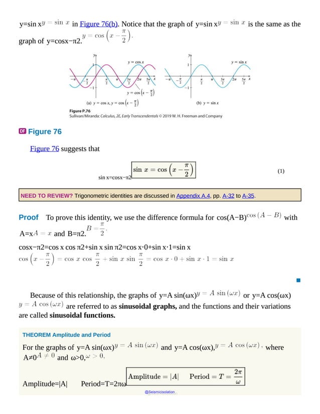
188. The range of f consists of all real numbers in the closed interval [−1,1].
The cosine function is an even function, so its graph is symmetric with respect to the y
-axis.
The cosine function has a period of 2π.
The x -intercepts of f are …,−3π2, −π2, π2, 3π2, 5π2,…
; the y -intercept is 1.
The maximum value of f is 1 and occurs at x=…,−2π, 0, 2π, 4π,
6π,… ; the minimum value of f is −1 and occurs at x=…,−π,
π, 3π, 5π,….
Many variations of the sine and cosine functions can be graphed using transformations.
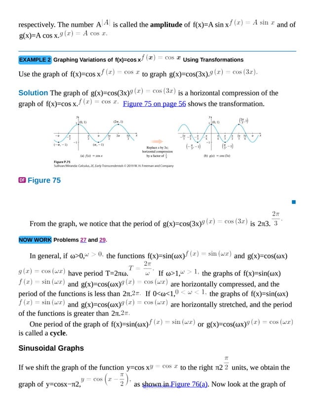
EXAMPLE 1 Graphing Variations of f(x)=sin x Using Transformations
Use the graph of f(x)=sin x to graph g(x)=2 sin x.
Solution Notice that g(x)=2 f(x), so the graph of g is a vertical stretch of
the graph of f(x)=sin x. Figure 74 illustrates the transformation.
Figure 74
▪
Notice that the values of g(x)=2 sin x lie between −2 and 2,
inclusive.
In general, the values of the functions f(x)=A sin x and g(x)=A cos x,
where A≠0, will satisfy the inequalities
−|A|≤A sin x≤|A| and −|A|≤A cos x≤|A|
@Seismicisolation
@Seismicisolation

189. respectively. The number A is called the amplitude of f(x)=A sin x and of
g(x)=A cos x.
EXAMPLE 2 Graphing Variations of f(x)=cos x Using Transformations
Use the graph of f(x)=cos x to graph g(x)=cos(3x).
Solution The graph of g(x)=cos(3x) is a horizontal compression of the
graph of f(x)=cos x. Figure 75 on page 56 shows the transformation.
Figure 75
▪
From the graph, we notice that the period of g(x)=cos(3x) is 2π3.
NOW WORK Problems 27 and 29.
In general, if ω>0, the functions f(x)=sin(ωx) and g(x)=cos(ωx)
have period T=2πω. If ω>1, the graphs of f(x)=sin(ωx)
and g(x)=cos(ωx) are horizontally compressed, and the
period of the functions is less than 2π. If 0<ω<1, the graphs of f(x)=sin(ωx)
and g(x)=cos(ωx) are horizontally stretched, and the period
of the functions is greater than 2π.
One period of the graph of f(x)=sin(ωx) or g(x)=cos(ωx)
is called a cycle.
Sinusoidal Graphs
If we shift the graph of the function y=cos x to the right π2 units, we obtain the
graph of y=cosx−π2, as shown in Figure 76(a). Now look at the graph of
@Seismicisolation
@Seismicisolation

190. y=sin x in Figure 76(b). Notice that the graph of y=sin x is the same as the
graph of y=cosx−π2.
Figure 76
Figure 76 suggests that
sin x=cosx−π2
(1)
NEED TO REVIEW? Trigonometric identities are discussed in Appendix A.4, pp. A-32 to A-35.
Proof To prove this identity, we use the difference formula for cos(A−B) with
A=x and B=π2.
cosx−π2=cos x cos π2+sin x sin π2=cos x⋅0+sin x⋅1=sin x
▪
Because of this relationship, the graphs of y=A sin(ωx) or y=A cos(ωx)
are referred to as sinusoidal graphs, and the functions and their variations
are called sinusoidal functions.
THEOREM Amplitude and Period
For the graphs of y=A sin(ωx) and y=A cos(ωx), where
A≠0 and ω>0,
Amplitude=|A| Period=T=2πω
@Seismicisolation
@Seismicisolation

191. EXAMPLE 3 Finding the Amplitude and Period of a Sinusoidal Function
Determine the amplitude and period of y=−3 sin(4πx).
Solution Comparing y=−3 sin(4πx) to y=A sin(ωx), we
find that A=−3 and ω=4π. Then,
Amplitude=|A|=|−3|=3 Period=T=2πω=2π4π=12
▪
NOW WORK Problem 33.
The function y=tanx is an odd function with period π. It is not defined at odd
multiples of π2. Do you see why? So, we construct Table 8 for 0≤x≤π3. Then
we plot the points from Table 8, connect them with a smooth curve, and reflect the graph
about the origin, as shown in Figure 77. To investigate the behavior of tan x near π2,
we use the identity tan x=sin xcos x. When x is close to, but less than, π2,
sin x is close to 1 and cos x is a positive number close to 0, so the ratio
sin xcos x is a large, positive number. The closer x gets to π2, the larger tan x
becomes. Figure 78 shows the graph of y=tanx, −π2<x<π2.
The graph of y=tanx is obtained by repeating the graph in Figure 78. See Figure 79.
TABLE 8
x y=tanx (x,y)
0 0 (0, 0)
π6 33 π6,33
π4
1
π4,1
π3 3
π3,3
@Seismicisolation
@Seismicisolation

192. Figure 77 y= tan x,−π3≤x≤π3
Figure 78 y= tan x,−π2<x<π2
@Seismicisolation
@Seismicisolation

193. Figure 79 y= tan x,−∞<x<∞, x≠ odd multiples of π2
The graph of y= tan x illustrates the following properties of the tangent
function:
Properties of the Tangent Function f(x)= tan x
The domain of f is the set of all real numbers, except odd multiples of π2.
The range of f consists of all real numbers.
The tangent function is an odd function, so its graph is symmetric with respect to the
origin.
The tangent function is periodic with period π.
The x -intercepts of f are …,−2π, −π, 0, π, 2π, 3π,… ;
the y -intercept is 0.
EXAMPLE 4 Graphing Variations of f(x)=tanx Using
Transformations
Use the graph of f(x)= tan x to graph g(x)=−tanx+π4.
Solution Figure 80 illustrates the steps used in graphing g(x)=−tan x+π4.
@Seismicisolation
@Seismicisolation

194. Begin by graphing f(x)=tanx. See Figure 80(a).
Replace the argument x by x+π4 to obtain y=tanx+π4, which
shifts the graph horizontally to the left π4 unit, as shown in Figure 80(b).
Multiply tan x+π4 by −1, which reflects the graph about the x -axis
and results in the graph of y=−tan x+π4, as shown in Figure 80(c).
Figure 80
First
figure
shows
the
graph
of
tan
x.
In
the
second
figure,
graph
is
shifted
left
by
▪
NOW WORK Problem 31.
The graph of the cotangent function is obtained similarly. y=cotx is an odd
function, with period π. Because cot x is not defined at multiples of π, graph y
on the interval (0,π) and then repeat the graph, as shown in Figure 81.
@Seismicisolation
@Seismicisolation

195. Figure 81 f(x)=cotx,−∞<x<∞, x≠ multiples of π
The cosecant and secant functions, sometimes referred to as reciprocal functions, are
graphed by using the reciprocal identities
csc x=1sin x and sec x=1cos x
The graphs of y= csc x and y= sec x are shown in Figures 82 and 83,
respectively.
Figure 82
@Seismicisolation
@Seismicisolation

196. Figure 83
P.6 Assess Your Understanding
Concepts and Vocabulary
1. The sine, cosine, cosecant, and secant functions have period ; the
tangent and cotangent functions have period .
2. The domain of the tangent function f(x)=tanx is .
3. The range of the sine function f(x)=sin x is .
4. Explain why tan π4+2π=tan π4.
5. True or False The range of the secant function is the set of all positive real numbers.
6. The function f(x)=3 cos(6x) has amplitude and
period .
7. True or False The graphs of y=sin x and y=cos x are identical except
for a horizontal shift.
8. True or False The amplitude of the function f(x)=2 sin(πx) is 2 and
its period is π2.
9. True or False The graph of the sine function has infinitely many x -intercepts.
10. The graph of y=tanx is symmetric with respect to the .
@Seismicisolation
@Seismicisolation

197. 11. The graph of y=sec x is symmetric with respect to the .
12. Explain, in your own words, what it means for a function to be periodic.
Practice Problems
In Problems 13–16, use the even-odd properties to find the exact value of each expression.
13. tan −π4
14. sin−3π2
15. csc−π3
16. cos−π6
In Problems 17–20, if necessary, refer to a graph to answer each question.
17. What is the y -intercept of f(x)=tanx ?
18. Find the x -intercepts of f(x)=sin x on the interval [−2π,2π].
19. What is the smallest value of f(x)=cos x ?
20. For what numbers x, −2π≤x≤2π, does sin x=1 ? Where in the
interval [−2π,2π] does sin x=−1 ?
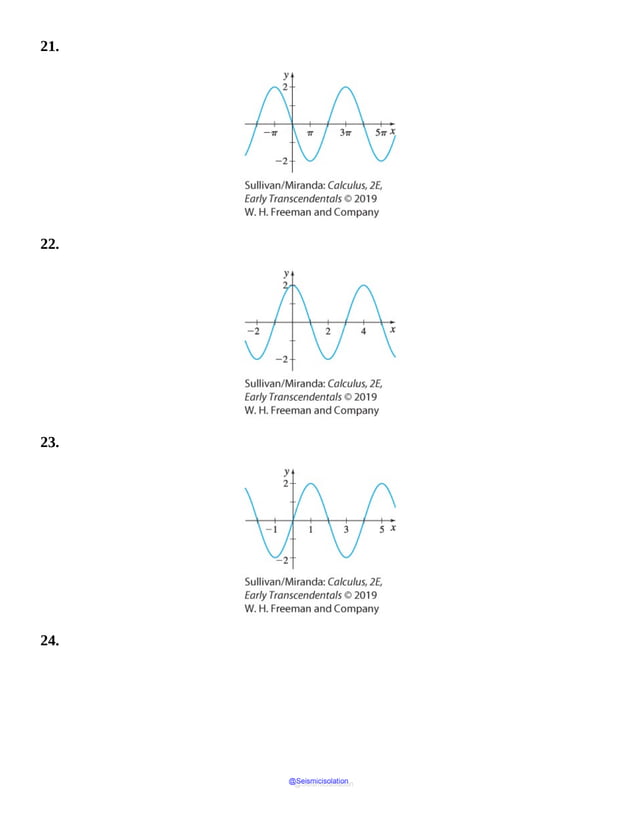
In Problems 21–26, the graphs of six trigonometric functions are given. Match each graph to
one of the following functions:
a. y=2 sinπ2 x
b. y=2 cosπ2 x
c. y=3 cos(2x)
d. y=−3 sin(2x)
e. y=−2 cosπ2 x
f. y=−2 sin12 x
@Seismicisolation
@Seismicisolation

198. 21.
22.
23.
24.
@Seismicisolation
@Seismicisolation

199. 25.
26.
In Problems 27–32, graph each function using transformations. Be sure to label key points
and show at least two periods.
27. f(x)=4 sin(πx)
28. f(x)=−3 cos x
29. f(x)=3 cos(2x)−4
30. f(x)=4 sin(2x)+2
@Seismicisolation
@Seismicisolation

200. 31. f(x)=tan π2 x
32. f(x)=4 sec12 x
In Problems 33–36, determine the amplitude andperiod of each function.
33. g(x)=12 cos(πx)
34. f(x)=sin(2x)
35. g(x)=3 sin x
36. f(x)=−2 cos32 x
In Problems 37 and 38, write the sine function that has the given properties.
37. Amplitude: 2, Period: π
38. Amplitude: 13, Period: 2
In Problems 39 and 40, write the cosine function that has the given properties.
39. Amplitude: 12, Period: π
40. Amplitude: 3, Period: 4π
In Problems 41–48, for each graph, find an equation involving the indicated trigonometric
function.
41.
@Seismicisolation
@Seismicisolation

201. 42.
43.
44.
@Seismicisolation
@Seismicisolation

202. 45.
46.
47.
@Seismicisolation
@Seismicisolation

203. 48.
1. = NOW WORK problem
= Graphing technology recommended
= Computer Algebra System recommended
@Seismicisolation
@Seismicisolation

204. P.7 Inverse Trigonometric Functions
OBJECTIVES When you finish this section, you should be able to:
1 Define the inverse trigonometric functions
2 Use the inverse trigonometric functions
3 Solve trigonometric equations
In Section P.4 we discussed inverse functions, and we concluded that if a function is one-to-
one, it has an inverse function. We also observed that if a function is not one-to-one, it may
be possible to restrict its domain so that the restricted function is one-to-one. For example,
the function y=x2 is not one-to-one. However, if we restrict the domain to x≥0,
the function is one-to-one.
Other properties of a one-to-one function f and its inverse function f−1 that we
discussed in Section P.4 are summarized below.
f−1 (f(x))=x for every x in the domain of f.
f(f−1 (x))=x for every x in the domain of f−1.
Domain of f=range of f−1 and range of f=domain of f−1.
The graph of f and the graph of f−1 are reflections of one another about the line
y=x.
If a function y=f(x) has an inverse function, the implicit equation of the
inverse function is x=f(y). If we solve this equation for y, we obtain the
explicit form y=f−1 (x).
We now investigate the inverse trigonometric functions. In calculus the inverses of the sine
function, the tangent function, and the secant function are used most often. So we define
these inverse functions first.
1 Define the Inverse Trigonometric Functions
Although the trigonometric functions are not one-to-one, we can restrict the domains of the
trigonometric functions so that each new function will be one-to-one on its restricted domain.
Then an inverse function can be defined on each restricted domain.
@Seismicisolation
@Seismicisolation

205. Figure 84 shows the graph of y=sin x. Because every horizontal line y=b,
where b is between −1 and 1, inclusive, intersects the graph of y=sin x
infinitely many times, it follows from the Horizontal-line Test that the function y=sin x
is not one-to-one.
Figure 84 y=sin x,−∞<x<∞,−1≤y≤1
The Inverse Sine Function
However, if the domain of the function f(x)=sin x is restricted to the interval
−π2,π2, the function y=sin x, −π2≤x≤π2, is one-to-one and
has an inverse function. See Figure 85.
@Seismicisolation
@Seismicisolation

206. Figure 85
To obtain an equation for the inverse of y=sin x on −π2≤x≤π2, we
interchange x and y. Then the implicit form of the inverse is x=sin y,
−π2≤y≤π2. The explicit form of the inverse function is called the inverse sine
of x and is written y=sin−1x.
DEFINITION Inverse Sine Function
The inverse sine function, denoted by y=sin−1x, or y=arcsinx, is
defined as
y= sin−1x if and only if x=sin ywhere −1≤x≤1 and −π2≤y≤π2
IN WORDS We read y=sin−1x as “y is the number (or angle) whose sine equals x.”
CAUTION The superscript −1 that appears in y= sin−1x is not an exponent but
the symbol used to denote the inverse function. (To avoid confusion, y= sin−1x is
@Seismicisolation
@Seismicisolation

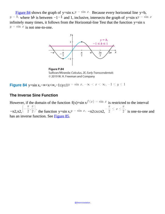
207. sometimes written y=arcsin x. )
The domain of y= sin−1x is the closed interval [−1,1], and the range is
the closed interval −π2,π2. The graph of y= sin−1x is the reflection of
the restricted portion of the graph of f(x)=sin x about the line y=x. See
Figure 86.
Figure 86
Sin
x
is
concave
up
in
the
first
quadrant
and
concave
up
in
the
Because y=sin x defined on the closed interval −π2,π2 and y= sin−1x
are inverse functions,
sin−1(sin x)=x if x is in the closed interval −π2,π2
sin(sin−1x)=x if x is in the closed interval [−1,1]
EXAMPLE 1 Finding the Values of an Inverse Sine Function
Find the exact value of:
a. sin−132
b. sin−1−22
@Seismicisolation
@Seismicisolation

208. c. sin−1sin π8
d. sin−1sin 5π8
Solution a. We seek an angle whose sine is 32. Let y= sin−132. Then
by definition, sin y=32, where −π2≤y≤π2. Although sin y=32
has infinitely many solutions, the only number in the interval −π2,π2
for which sin y=32, is π3. So sin−132=π3.
b. We seek an angle whose sine is −22. Let y= sin−1−22. Then by
definition, sin y=−22, where −π2≤y≤π2. The only number in the
interval −π2,π2 whose sine is −22, is −π4. So sin−1−22=−π4.
c. Since the number π8 is in the interval −π2,π2, we use (1).
sin−1sin π8=π8
d. Since the number 5π8 is not in the closed interval −π2,π2, we cannot use (1).
Instead, we find a number x in the interval −π2,π2 for which sin x=sin 5π8.
Using Figure 87, we see that sin 5π8=y=sin 3π8. The
number 3π8 is in the interval −π2,π2, so
sin−1sin 5π8= sin−1sin 3π8=3π8
@Seismicisolation
@Seismicisolation

209. Figure 87
▪
NOW WORK Problems 9 and 21.
The Inverse Tangent Function
The tangent function y= tan x is not one-to-one. To define the inverse tangent
function, we restrict the domain of y= tan x to the open interval −π2,π2.
On this interval, y= tan x is one-to-one. See Figure 88.
@Seismicisolation
@Seismicisolation

210. Figure 88
Now use the steps for finding the inverse of a one-to-one function, listed on page 39:
Step 1 y= tan x, −π2<x<π2.
Step 2 Interchange x and y to obtain x= tan y, −π2<y<π2, the
implicit form of the inverse tangent function.
Step 3 The explicit form is called the inverse tangent of x and is denoted by y= tan−1x.
DEFINITION Inverse Tangent Function
The inverse tangent function, symbolized by y= tan−1x, or y=arctanx,
is
y=tan−1x if and only if x= tan ywhere −∞<x<∞ and −π2<y<π2
The domain of the function y= tan−1x is the set of all real numbers, and its
range is −π2<y<π2. To graph y= tan−1x, reflect the graph of
@Seismicisolation
@Seismicisolation

211. y= tan x, −π2<x<π2, about the line y=x, as shown in Figure
89.
Figure 89
Tan
x
is
concave
up
in
the
first
quadrant
and
concave
down
in
the
third
quadrant.
Arctanx
is
NOW WORK Problem 13.
The Inverse Secant Function
To define the inverse secant function, we restrict the domain of the function y= sec x
to the set [0,π2)∪[π,3π2). See Figure 90(a) on page 64. An
equation for the inverse function is obtained by following the steps for finding the inverse of
a one-to-one function. By interchanging x and y, we obtain the implicit form of the
inverse function: x= sec y, where 0≤y<π2 or π≤y<3π2.
The explicit form is called the inverse secant of x and is written y= sec−1x.
The graph of y= sec−1x is given in Figure 90(b).
@Seismicisolation
@Seismicisolation

212. Figure 90
Sec
x
is
concave
up
from
point
(0,
1)
on
the
interval
[0,
0.5
pi)
and
concave
down
from
(pi,
minus
1)
on
DEFINITION Inverse Secant Function
The inverse secant function, symbolized by y= sec−1x, or y=arcsecx,
is
y= sec−1x if and only if x= sec ywhere | x|≥1 and 0≤y<π2 or π≤y<3π2
You may wonder why we chose the restriction we did to define y= sec−1x.
The reason is that this restriction not only makes y= sec x one-to-one, but it also
makes tan x≥0. With tan x≥0, the derivative formula for the inverse
secant function is simpler, as we will see in Chapter 3.
The remaining three inverse trigonometric functions are defined as follows.
DEFINITION
Inverse Cosine Function y= cos−1x if and only if x=cos y
where −1≤x≤1 and 0≤y≤π
Inverse Cotangent Function y= cot−1x if and only if x=cot y
@Seismicisolation
@Seismicisolation

213. where −∞<x<∞ and 0<y<π
Inverse Cosecant Function y= csc−1x if and only if x=csc y
where | x|≥1 and −π<y≤−π2 or
0<y≤π2
The following three identities involve the inverse trigonometric functions. The proofs
may be found in books on trigonometry.
THEOREM
cos−1x=π2−sin−1x, −1≤x≤1
cot−1x=π2−tan−1x, −∞<x<∞
csc−1x=π2−sec−1x, | x|≥1
The identities above are used whenever the inverse cosine, inverse cotangent, and inverse
cosecant functions are needed. The graphs of the inverse cosine, inverse cotangent, and
inverse cosecant functions can also be obtained by using these identities to transform the
graphs of y= sin−1x, y= tan−1x, and y= sec−1x,
respectively.
2 Use the Inverse Trigonometric Functions
EXAMPLE 2 Writing a Trigonometric Expression as an Algebraic Expression
Write sin(tan−1u) as an algebraic expression containing u.
Solution Let θ= tan−1u so that tan θ=u, where −π2<θ<π2.
We note that in the interval −π2,π2, sec θ>0. Then
@Seismicisolation
@Seismicisolation

214. Sine
open
parentheiss
tangent
inverse
of
u
close
parenthesis
equals
sine
theta
equals
sine
theta
times
cosine
theta
over
cosine
theta
equals
tangent
theta
cosine
thet
Equals
tangent
theta
over
secant
theta
equals
tangent
theta
over
square
root
of
1
An alternate method of obtaining the solution to Example 2 uses right triangles. Let
θ= tan−1u so that tan θ=u, −π2<θ<π2, and label the right
triangles drawn in Figure 91. Using the Pythagorean Theorem, the hypotenuse of each
triangle is 1+u2. Then sin(tan−1u)=sin θ=u1+u2.
Figure 91 tan θ=u ; −π2<θ<π2
NOW WORK Problem 67.
3 Solve Trigonometric Equations
Inverse trigonometric functions can be used to solve trigonometric equations.
EXAMPLE 3 Solving Trigonometric Equations
Solve the equations:
a. sin θ=12
b. cos θ=0.4
Give a general formula for all the solutions and list all the solutions in the interval [−2π,2π].
@Seismicisolation
@Seismicisolation

215. Solution a. Use the inverse sine function y= sin−1x, −π2≤y≤π2.
sin θ=12 θ= sin−112−π2≤θ≤π2 θ=π6
Over the interval [0,2π], one period, there are two angles θ for which sin θ=12:π6
and 5π6. See Figure 92. Using the period 2π, the solutions of sin θ=12
are given by the general formula
θ=π6+2kπ or θ=5π6+2kπ where k is any integer
Figure 92
The solutions in the interval [−2π,2π] are
−11π6,−7π6,π6,5π6
@Seismicisolation
@Seismicisolation

216. b. A calculator must be used to solve cos θ=0.4. With your calculator in radian
mode,
θ= cos−10.4≈1.159279 0≤θ≤π
Rounded to three decimal places, θ= cos−10.4=1.159 radians. But
there is another angle θ in the interval [0,2π] for which cos θ=0.4,
namely, θ≈2π−1.159≈5.124 radians.
Because the cosine function has period 2π, all the solutions of cos θ=0.4
are given by the general formulas
θ≈1.159+2kπ or θ≈5.124+2kπ where k is any integer
The solutions in the interval [−2π,2π] are −5.124,−1.159, 1.159, 5.124.
▪
NOW WORK Problem 63.
EXAMPLE 4 Solving a Trigonometric Equation
Solve the equation sin(2θ)=12, where 0≤θ<2π.
Solution In the interval 0,2π, the sine function has the value 12 at θ=π6 and
at θ=5π6, as shown in Figure 93. Since the period of the sine function is 2π and
the argument in the equation sin(2θ)=12 is 2θ, we write the general formula
for all the solutions.
2θ=π6+2kπor2θ=5π6+2kπwhere k is any integer θ=π12+kπ θ=5π12+kπ
@Seismicisolation
@Seismicisolation

217. Figure 93
The solutions of sin(2θ)=12, 0≤θ<2π, are π12, 5π12, 13π12, 17π12.
▪
NOW WORK Problem 49.
NEED TO REVIEW? Trigonometric identities are discussed in Appendix Section A.4, pp. A-32 to A-35.
Many trigonometric equations can be solved by applying algebra techniques such as
factoring or using the quadratic formula. It is often necessary to begin by using a
trigonometric identity to express the given equation in a familiar form.
EXAMPLE 5 Solving a Trigonometric Equation
Solve the equation 3 sin θ−cos2 θ=3, where 0≤θ<2π.
Solution The equation involves both sine and cosine functions. We use the Pythagorean
identity sin2 θ+cos2 θ=1 to rewrite the equation in terms of sin θ.
3 sin θ−cos2 θ=33 sin θ−(1−sin2 θ)=3 cos2 θ=1−sin2 θsin2 θ+3 sin θ−4=0
@Seismicisolation
@Seismicisolation

218. This is a quadratic equation in sin θ. Factor the left side and solve for sin θ.
(sin θ+4)(sin θ−1)=0sin θ+4=0orsin θ−1=0sin θ=−4orsin θ=1
The range of the sine function is −1≤y≤1, so sin θ=−4 has no solution.
Solving sin θ=1, we obtain
θ= sin−11=π2
The only solution in the interval 0,2π is π2. ▪
NOW WORK Problem 53.
P.7 Assess Your Understanding
Concepts and Vocabulary
1. y= sin−1x if and only if x= __________, where −1≤x≤1 and
−π2≤y≤π2.
2. True or False sin−1 (sin x)=x, where −1≤x ≤1.
3. True or False The domain of y= sin−1x is −π2≤x≤π2.
4. True or False sin(sin−1 0)=0.
5. True or False y= tan−1x means x= tan y, where −∞<x<∞
and −π2≤y≤π2.
6. True or False The domain of the inverse tangent function is the set of all real numbers.
7. True or False sec−10.5 is not defined.
8. True or False Trigonometric equations can have multiple solutions.
Practice Problems
In Problems 9–20, find the exact value of each expression. Do not use a calculator.
@Seismicisolation
@Seismicisolation

219. 9. sin−1 0
10. tan−1 1
11. sec−1 (−1)
12. sec−1 233
13. tan−1 (−1)
14. tan−1 0
15. sin−122
16. tan−133
17. tan−13
18. sin−1−32
19. sec−1 (−2)
20. sin−1−22
In Problems 21–28, find the exact value of each expression. Do not use a calculator.
21. sin−1sin π5
22. sin−1sin−π10
23. tan−1tan−3π8
24. sin−1sin 3π7
25. sin−1sin 9π8
@Seismicisolation
@Seismicisolation

220. 26. sin−1sin−5π3
27. tan−1tan 4π5
28. tan−1tan−2π3
In Problems 29–44, find the exact value, if any, of each composite function. If there is no
value, write, “It is not defined.” Do not use a calculator.
29. sinsin−114
30. sinsin−1−23
31. tan(tan−1 4)
32. tan[tan−1 (−2)]
33. sin(sin−1 1.2)
34. sin[sin−1 (−2)]
35. tan(tan−1π)
36. sin[sin−1 (−1.5)]
37. cos(sin−1 0.3)
38. sin(tan−1 2)
39. tan(sec−1 2)
40. cos(tan−1 3)
41. sin(sin−1 0.2+tan−1 2)
42. cos(sec−1 2+sin−1 0.1)
43. tan(2 sin−1 0.4)
44. cos(2 tan−1 5)
@Seismicisolation
@Seismicisolation

221. In Problems 45–62, solve each equation on the interval 0≤θ<2π.
45. tan θ=−33
46. sec 3θ2=−2
47. 2 sin θ+3=2
48. 1−cos θ=12
49. sin (3θ)=−1
50. cos(2θ)=12
51. 4 cos2 θ=1
52. 2 sin2 θ−1=0
53. 2 sin2 θ−5 sin θ+3=0
54. 2 cos2 θ−7 cos θ−4=0
55. 1+sin θ=2 cos2 θ
56. sec2 θ+tan θ=0
57. sin θ+cos θ=0
58. tan θ=cot θ
59. cos(2θ)+6 sin2 θ=4
60. cos(2θ)=cos θ
61. sin (2θ)+sin(4θ)=0
62. cos(4θ)−cos(6θ)=0
In Problems 63–66, use a calculator to solve each equation on the interval 0≤θ<2π.
Round answers to three decimal places.
63. tan θ=5
64. cos θ=0.6
65. 2+3 sin θ=0
@Seismicisolation
@Seismicisolation

222. 66. 4+sec θ=0
67. Write cos(sin−1u) as an algebraic expression containing u, where | u|≤1.
68. Write tan(sin−1u) as an algebraic expression containing u, where | u|≤1.
69. Show that y= sin−1x is an odd function. That is, show sin−1 (−x)=−sin−1x.
70. Show that y=tan−1x is an odd function. That is, show tan−1 (−x)=−tan−1x.
71. a. On the same set of axes, graph f(x)=3 sin(2x)+2 and g(x)=72
on the interval [0,π].
b. Solve f(x)=g(x) on the interval [0,π] and label the points of
intersection on the graph drawn in (a).
c. Shade the region bounded by f(x)=3 sin(2x)+2 and g(x)=72
between the points found in (b) on the graph drawn in (a).
d. Solve f(x)>g(x) on the interval [0,π].
72. a. On the same set of axes, graph f(x)=−4 cos x and g(x)=2 cos x+3
on the interval [0,2π].
b. Solve f(x)=g(x) on the interval [0,2π] and label the points of
intersection on the graph drawn in (a).
c. Shade the region bounded by f(x)=−4 cos x and g(x)=2 cos x+3
between the points found in (b) on the graph drawn in (a).
d. Solve f(x)>g(x) on the interval [0,2π].
73. Area Under a Graph The area A under the graph of y=11+x2 and above
the x -axis between x=a and x=b is given by
A=tan−1b−tan−1a
See the figure.
@Seismicisolation
@Seismicisolation

223. a. Find the exact area under the graph of y=11+x2 and above the x -axis
between x=0 and x=3.
b. Find the exact area under the graph of y=11+x2 and above the x -axis
between x=−33 and x=1.
74. Area Under a Graph The area A under the graph of y=11−x2 and
above the x -axis between x=a and x=b is given by
A=sin−1b−sin−1a
See the figure.
a. Find the exact area under the graph of y=11−x2 and above the x -axis
between x=0 and x=32.
@Seismicisolation
@Seismicisolation

224. b. Find the exact area under the graph of y=11−x2 and above the x -axis
between x=−12 and x=12.
1. = NOW WORK problem
= Graphing technology recommended
= Computer Algebra System recommended
@Seismicisolation
@Seismicisolation

225. P.8 Sequences; Summation Notation; the Binomial
Theorem
OBJECTIVES When you finish this section, you should be able to:
1 Write the first several terms of a sequence
2 Write the terms of a recursively defined sequence
3 Use summation notation
4 Find the sum of the first n terms of a sequence
5 Use the Binomial Theorem
When you hear the word sequence as used in “a sequence of events,” you probably think of
something that happens first, then second, and so on. In mathematics, the word sequence also
refers to outcomes that are first, second, and so on.
DEFINITION Sequence
A sequence is a function whose domain is the set of positive integers.
In a sequence the inputs are 1,2,3,…. Because a sequence is a function, it has a
graph. Figure 94(a) shows the graph of the function f(x)=1x,x>0. If all the
points on this graph are removed except those whose x -coordinates are positive integers,
that is, if all points are removed except (1,1), 2,12, 3,13, and so on,
the remaining points would be the graph of the sequence f(n)=1n, as shown in
Figure 94(b). Notice that we use n to represent the independent variable in a sequence. This
is to remind us that n is a positive integer.
@Seismicisolation
@Seismicisolation

226. Figure 94
1 Write the First Several Terms of a Sequence
A sequence is usually represented by listing its values in order. For example, the sequence
whose graph is given in Figure 94(b) might be represented as
f(1), f(2), f(3), f(4),…or1,12,13,14,…
The list never ends, as the dots (ellipses) indicate. The numbers in this ordered list are called
the terms of the sequence.
In dealing with sequences, we usually use subscripted letters such as a1 to represent
the first term, a2 for the second term, a3 for the third term, and so on.
For the sequence f(n)=1n, we write
a1=f(1)=1First terma2=f(2)=12Second terma3=f(3)=13Third terma4=f(4)=14⋯Fourth
terman=f(n)=1n⋯nth term
In other words, we usually do not use the traditional function notation f(n) for
sequences. For this particular sequence, we have a rule for the n th term, which is an=1n,
so it is easy to find any term of the sequence.
When a formula for the n th term (sometimes called the general term) of a sequence is
known, we usually represent the entire sequence by placing braces around the formula for the
n th term. For example, the sequence whose n th term is bn=12n can be
represented either as
@Seismicisolation
@Seismicisolation

227. b1=12,b2=14,b3=18, …, bn=12n, …,
or as
{bn}=12n
EXAMPLE 1 Writing the Terms of a Sequence
Write the first six terms of the sequence: {Sn}=(−1)n−12n
Solution S1=(−1)021=2S2=(−1)122=−1S3=(−1)223=23S4=−12S5=25S6=−13
The first six terms of the sequence are 2,−1, 23,−12, 25,−13. ▪
NOW WORK Problem 17.
EXAMPLE 2 Determining a Sequence from a Pattern
The pattern on the left suggests the n th term of the sequence on the right.
Pattern n th Term Sequence
e,e22,e33,e44,… an=enn {an}=enn
1, 13, 19, 127,… bn=13n−1
{bn}=13n−1
1, 3, 5, 7,… cn=2n−1 {cn}={2n−1}
1, 4, 9, 16, 25,… dn=n2 {dn}={n2}
1, −12, 13, −14, 15,… en=(−1)n+1 1n
{en}=(−1)n+1 1n
▪
@Seismicisolation
@Seismicisolation

228. NOW WORK Problem 21.
2 Write the Terms of a Recursively Defined Sequence
A second way of defining a sequence is to assign a value to the first (or the first few) term(s)
and specify the n th term by a formula or an equation that involves one or more of the terms
preceding it. Such a sequence is defined recursively, and the rule or formula is called a
recursive formula.
EXAMPLE 3 Writing the Terms of a Recursively Defined Sequence
Write the first five terms of the recursively defined sequence.
s1=1sn=4sn−1n≥2
Solution The first term is given as s1=1. To get the second term, we use n=2
in the formula to obtain s2=4s1=4⋅1=4. To obtain the third term, we use
n=3 in the formula, getting s3=4s2=4⋅4=16. Each new term
requires that we know the value of the preceding term. The first five terms are
s1=1s2=4s2−1=4s1=4⋅1=4s3=4s3−1=4s2=4⋅4=16s4=4s4−1=4s3=4⋅16=64s5=4s5−1=4s4=4⋅6
▪
NOW WORK Problem 29.
EXAMPLE 4 Writing the Terms of a Recursively Defined Sequence
Write the first five terms of the recursively defined sequence.
u1=1u2=1un=un−2+un−1n≥3
Solution We are given the first two terms. Obtaining the third term requires that we know
each of the previous two terms.
u1=1u2=1u3=u1+u2=1+1=2u4=u2+u3=1+2=3u5=u3+u4=2+3=5
@Seismicisolation
@Seismicisolation

229. ▪
The sequence defined in Example 4 is called a Fibonacci sequence; its terms are called
Fibonacci numbers. These numbers appear in a wide variety of applications.
NOW WORK Problem 35.
3 Use Summation Notation
It is often important to be able to find the sum of the first n terms of a sequence {an},
namely,
a1+a2+a3+⋯+an
Rather than write down all these terms, we introduce summation notation. Using
summation notation, the sum is written
a1+a2+a3+⋯+an=∑k=1nak
NOTE Summation notation is called sigma notation in some books.
The symbol ∑ (the uppercase Greek letter sigma, which is an S in our alphabet) is
simply an instruction to sum, or add up, the terms. The integer k is called the index of
summation; it tells us where to start the sum (k=1) and where to end it (k=n).
The expression ∑k=1nak is read, “The sum of the terms ak from k=1
to k=n. ”
EXAMPLE 5 Expanding Summation Notation
Write out each sum:
a. ∑k=1n1k
@Seismicisolation
@Seismicisolation

230. b. ∑k=1nk!
NOTE If n≥0 is an integer, the factorial symbol ! means 0!=1, 1!=1, and n!=1⋅2⋅3⋅ ⋯
⋅(n−1)⋅n, where n>1.
Solution a. ∑k=1n1k=1+12+13+⋯+1n
b. ∑k=1nk!=1!+2!+⋯+n! ▪
NOW WORK Problem 41.
EXAMPLE 6 Writing a Sum in Summation Notation
Express each sum using summation notation:
a. 12+22+32+⋯+92
b. 1+12+14+18+⋯+12n−1
Solution a. The sum 12+22+32+⋯+92 has 9 terms, each of the
form k2; it starts at k=1 and ends at k=9:
12+22+32+⋯+92=∑k=19k2
b. The sum
1+12+14+18+⋯+12n−1
has n terms, each of the form 12k−1. It starts at k=1 and ends at k=n.
1+12+14+18+⋯+12n−1=∑k=1n12k−1
▪
The index of summation does not need to begin at 1 or end at n. For example, the
@Seismicisolation
@Seismicisolation

231. sum in Example 6(b) could be expressed as
∑k=0n−112k=1+12+14+18+⋯+12n−1
Letters other than k can be used as the index. For example,
∑j=1nj!and∑i=1ni!
each represent the same sum as Example 5(b).
NOW WORK Problem 51.
4 Find the Sum of the First n Terms of a Sequence
When working with summation notation, the following properties are useful for finding the
sum of the first n terms of a sequence.
THEOREM Properties Involving Summation Notation
If {an} and {bn} are two sequences and c is a real number, then:
The proof of property (1) follows from the distributive property of real numbers. The
proofs of properties (2) and (3) are based on the commutative and associative properties of
real numbers. Property (4) states that the sum from j+1 to n equals the sum from 1 to
n minus the sum from 1 to j. It can be helpful to use this property when the index of
summation begins at a number larger than 1.
THEOREM Formulas for Sums of the First n Terms of a Sequence
@Seismicisolation
@Seismicisolation

232. Notice the difference between formulas (5) and (6). In formula (5), the constant 1 is
being summed from 1 to n, while in (6), the index of summation k is being summed
from 1 to n.
EXAMPLE 7 Finding Sums
Find each sum:
a. ∑k=110012
b. ∑k=15(3k)
c. ∑k=110(k3+1)
d. ∑k=620(4k2)
Solution a.
The
summation
of
k
equals
b.
The
sumation
c.
@Seismicisolation
@Seismicisolation

233. d. Notice that the index of summation starts at 6.
The
summation
of
k
equals
6
to
20
of
4
k
squared
equals
4
the
summation
of
k
equals
6
to
20
of
k
squared
equals
4
open
bracket
the
summation
of
k
▪
NOW WORK Problem 61.
5 Use the Binomial Theorem
You already know formulas for expanding (x+a)n for n=2 and n=3.
The Binomial Theorem is a formula for the expansion of (x+a)n for any positive
integer n.
If n=1, 2 , 3 , and 4 , the expansion of (x+a)n is straightforward.
•(x+a)1=x+aTwo terms, beginning with x1 and ending with a1•(x+a)2=x2+2ax+a2Three
terms, beginning with x2 and ending with a2•(x+a)3=x3+3ax2+3a2x+a3Four terms,
beginning with x3 and ending with a3•(x+a)4=x4+4ax3+6a2x2+4a3x+a4Five terms,
beginning with x4 and ending with a4
Notice that each expansion of (x+a)n begins with xn, ends with an, and
has n+1 terms. As you look at the terms from left to right, the powers of x are
decreasing by one, while the powers of a are increasing by one. As a result, we might
conjecture that the expansion of (x+a)n would look like this:
(x+a)n=xn+_______axn−1+_______a2xn−2+⋯+_______an−1x+an
where the blanks are numbers to be found. This, in fact, is the case.
Before filling in the blanks, we introduce the symbol (nj).
DEFINITION @Seismicisolation
@Seismicisolation

234. If j and n are integers with 0≤j≤n, the symbol (nj) is defined as
(nj)=n!j! (n−j)!
EXAMPLE 8 Evaluating (nj)
a. (31)=3!1!(3−1)!=3!1!2!=3⋅2⋅11(2⋅1)=62=3
b. (42)=4!2!(4−2)!=4!2!2!=4⋅3⋅2⋅1(2⋅1)(2⋅1)=244=6
c.
1
cross
1
matrix:
row
1,
column
1
reads:
8;
row
2,
column
1
reads:
7;
equals
8
exclamation
mark
d. (n0)=n!0!(n−0)!=n!0!n!=n!1⋅n!=1
e. (nn)=n!n!(n−n)!=n!n!0!=n!n!⋅1=1 ▪
RECALL 0!=1
NOW WORK Problem 67.
THEOREM Binomial Theorem
Let x and a be real numbers. For any positive integer n,
(x+a)n=(n0)xn+(n1)axn−1+(n2)a2xn−2+⋯+(nj)ajxn−j+⋯+(nj)an=∑j=0n(nj)ajxn−j
@Seismicisolation
@Seismicisolation

235. Because of its appearance in the Binomial Theorem, the symbol (nj) is called a
binomial coefficient.
EXAMPLE 9 Expanding a Binomial
Use the Binomial Theorem to expand (x+2)5.
Solution We use the Binomial Theorem with a=2 and n=5. Then
(x+2)5=(50)x5+(51)2x4+(52)22x3+(53)23x2+(54)24x+
(55)25=1⋅x5+5⋅2x4+10⋅4x3+10⋅8x2+5⋅16x+1⋅32=x5+10x4+40x3+80x2+80x+32
▪
NOW WORK Problem 77.
P.8 Assess Your Understanding
Concepts and Vocabulary
1. A(n)__________ is a function whose domain is the set of positive integers.
2. True or False 3!=6
3. If n≥0 is an integer, then n!=______________ when n≥2.
4. The sequence a1=5, an=3an−1 is an example of a(n)__________
sequence.
5. The notation a1+a2+a3+⋯+an=∑k=1nak is an
example of__________ notation.
6. True or False ∑k=1nk=1+2+3+⋯+n=n(n+1)2
@Seismicisolation
@Seismicisolation

236. 7. If s1=1 and sn=4sn−1, then s3=______________.
8. (n0)=______________; (n1)=______________
9. True or False (nj)=j!(n−j)!n!
10. The__________ can be used to expand expressions like (2x+3)6.
Practice Problems
In Problems 11–18, write the first five terms of each sequence.
11. {sn}={2n}
12. {sn}={n2}
13. {an}=nn+1
14. {an}=n+12n
15. {bn}={(−1)nn2}
16. {bn}=(−1)n−1nn+1
17. {sn}=(−1)n−12n3n+1
18. {sn}=(−1)n−143n
In Problems 19–26, the given pattern continues. Find the nth term of a sequence suggested
by the pattern.
19. 2,32,43,54,…
20. 12⋅3,13⋅4,14⋅5,15⋅6,…
@Seismicisolation
@Seismicisolation

237. 21. 1,14,19,116,125,⋯
22. 13,25,37,49,511,⋯
23. 2,−4,6,−8,10,…
24. 2,−2,2,−2,2,…
25. 2,−3,4,−5,6,…
26. 1,12,3,14,5,16,7,18,⋯
In Problems 27–38, a sequence is defined recursively. Write the first five terms of the
sequence.
27. a1=3;an=2+an−1
28. a1=1;an=4+an−1
29. a1=2;an=n+an−1
30. a1=−1;an=n+an−1
31. a1=1;an=3an−1
32. a1=1;an=−an−1
33. a1=2;an=an−1n
34. a1=−3;an=n+an−1
35. a1=1;a2=−1;an=an−1⋅an−2
36. a1=−1;a2=2;an=an−2+nan−1
37. a1=A;an=an−1+d
38. a1=A;an=ran−1,r≠0
In Problems 39–48, write out each sum.
39. ∑k=1n(k−2)
40. ∑k=1n(2k)
@Seismicisolation
@Seismicisolation

238. 41. ∑k=1nk2k+1
42. ∑k=1n(k+1)2k
43. ∑k=0n12k
44. ∑k=0n23k
45. ∑k=0nk+12k+1
46. ∑k=1n2k+2k
47. ∑k=2n(−1)k2k
48. ∑k=1n(−1)k+1 ln k
In Problems 49–56, express each sum using summation notation.
49. 2+4+6+⋯+100
50. 12+232+332+⋯+732
51. 2+32+43+⋯+35+135
52. 32+52+72+92+⋯+2(12)+12
53. 3−310+3100−31000+⋯+(−1)1031010
54. −23+29−227+⋯+(−1)8238
@Seismicisolation
@Seismicisolation

239. 55. 1e−2e2+3e3−⋯+(−1)n+1nen
56. 1−52+523−534+⋯+(−1)n−15n−1n
In Problems 57–66, find the sum of each sequence.
57. ∑k=12545
58. ∑k=1506
59. ∑k=130(3k)
60. ∑k=120 −2k3
61. ∑k=1100(2k−1)
62. ∑k=118(4k+3)
63. ∑k=120(k2−2)
64. ∑k=010(k2+1)
65. ∑k=650 k2
66. ∑k=320(3k)
In Problems 67–72, evaluate each expression.
@Seismicisolation
@Seismicisolation

240. 67. (52)
68. (74)
69. (93)
70. (84)
71. (501)
72. (1002)
In Problems 73–80, expand each expression using the Binomial Theorem.
73. (x+1)4
74. (x−1)6
75. (x−3)5
76. (x+2)4
77. (2x+3)4
78. (2x−1)5
79. (x2−y2)3
80. (x2+y2)4
81. Credit Card Debt John has a balance of $3000 on his Discover card that charges
1% interest per month on any unpaid balance. John can afford to pay $100
toward the balance each month. His balance each month after making a $100
payment is given by the recursively defined sequence
B0=$3000Bn=1.01Bn−1−100
Determine John’s balance after making the first payment. That is, determine B1.
@Seismicisolation
@Seismicisolation

241. 82. Approximating f(x) = ex In calculus it can be shown that
f(x)=ex=∑k=0∞xkk!
We can approximate the value of f(x)=ex for any x using the sum
f(x)=ex≈∑k=0nxkk!
for some n.
a. Approximate f(1.3) with n=4.
b. Approximate f(1.3) with n=7.
c. Use a calculator to approximate f(1.3).
d. Use trial and error along with a graphing calculator’s SEQuence mode to
determine the value of n required to approximate f(1.3) correct to eight
decimal places.
1. = NOW WORK problem
= Graphing technology recommended
= Computer Algebra System recommended
@Seismicisolation
@Seismicisolation

242. 1 Limits and Continuity
1.1 Limits of Functions Using Numerical and Graphical Techniques
1.2 Limits of Functions Using Properties of Limits
1.3 Continuity
1.4 Limits and Continuity of Trigonometric, Exponential, and Logarithmic Functions
1.5 Infinite Limits; Limits at Infinity; Asymptotes
1.6 The ε–δ Definition of a Limit
Chapter Review
Chapter Project
Oil Spills and Dispersant Chemicals
On April 20, 2010, the Deepwater Horizon drilling rig exploded and initiated the
worst marine oil spill in recent history. Oil gushed from the well for three months
and released millions of gallons of crude oil into the Gulf of Mexico. One technique
used to help clean up during and after the spill was the use of the chemical
dispersant Corexit, pictured above in the waters off the coast of Louisiana. Oil
dispersants allow the oil particles to spread more freely in the water, thus allowing
the oil to biodegrade more quickly. Their use is debated, however, because some
of their ingredients are carcinogens. Further, the use of oil dispersants can
increase toxic hydrocarbon levels affecting sea life. Over time, the pollution
@Seismicisolation
@Seismicisolation

243. caused by the oil spill and the dispersants will eventually diminish and sea life will
return, more or less, to its previous condition. In the short term, however, pollution
raises serious questions about the health of the local sea life and the safety of fish
and shellfish for human consumption.
CHAPTER 1 PROJECT The Chapter Project on page 152 looks at a hypothetical
situation involving pollution in a lake and explores some legal arguments that might
be made.
The concept of a limit is central to calculus. To understand calculus, it is essential to know
what it means for a function to have a limit, and then how to find a limit of a function.
Chapter 1 explains what a limit is, shows how to find a limit of a function, and demonstrates
how to prove that limits exist using the definition of limit.
We begin the chapter using numerical and graphical approaches to explore the idea of a
limit. Although these methods seem to work well, there are instances in which they fail to
identify the correct limit.
In Section 1.2, we use analytic techniques to find limits. Some of the proofs of these
techniques are found in Section 1.6, others in Appendix B. A limit found by correctly
applying these analytic techniques is precise; there is no doubt that it is correct.
In Sections 1.3–1.5, we continue to study limits and some ways that they are used. For
example, we use limits to define continuity, an important property of a function.
Section 1.6 provides a precise definition of limit, the so-called ε‑δ (epsilon-delta)
definition, which we use to show when a limit does, and does not, exist.
@Seismicisolation
@Seismicisolation

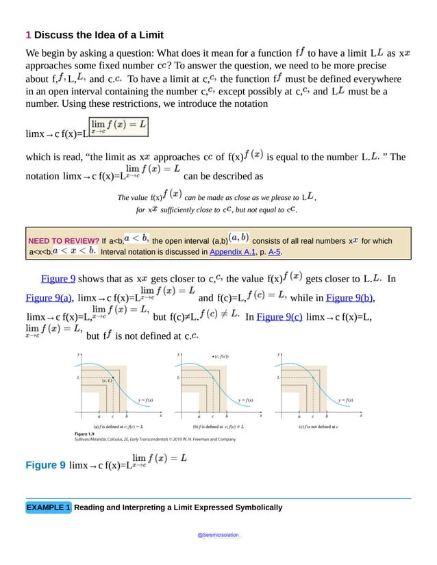
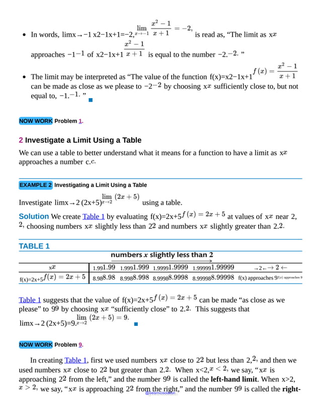
244. 1.1 Limits of Functions Using Numerical and Graphical
Techniques
OBJECTIVES When you finish this section, you should be able to:
1 Discuss the idea of a limit
2 Investigate a limit using a table
3 Investigate a limit using a graph
Calculus can be used to solve certain fundamental questions in geometry. Two of these
questions are:
Given a function f and a point P on its graph, what is the slope of the tangent line to
the graph of f at P ? See Figure 1.
Given a nonnegative function f whose domain is the closed interval [a,b], what is
the area of the region enclosed by the graph of f, the x -axis, and the vertical lines
x=a and x=b ? See Figure 2.
Figure 1
@Seismicisolation
@Seismicisolation

245. Figure 2
These questions, traditionally called the tangent problem and the area problem, were
solved by Gottfried Wilhelm von Leibniz and Sir Isaac Newton during the late seventeenth
and early eighteenth centuries. The solutions to the two seemingly different problems are
both based on the idea of a limit. Their solutions not only are related to each other but are
also applicable to many other problems in science and geometry. Here we begin to discuss
the tangent problem. The discussion of the area problem begins in Chapter 5.
The Slope of the Tangent Line to a Graph
Notice that the line ℓT in Figure 1 just touches the graph of f at the point P. This
unique line is the tangent line to the graph of f at P. But how is the tangent line defined?
In plane geometry, a tangent line to a circle is defined as a line having exactly one point
in common with the circle, as shown in Figure 3. However, this definition does not work for
graphs in general. For example, in Figure 4, the three lines ℓ1, ℓ2, and ℓ3 contain the
point P and have exactly one point in common with the graph of f, but they do not meet
the requirement of just touching the graph at P. On the other hand, the line ℓT just
touches the graph of f at P, but it intersects the graph at another point. It is the slope of
the tangent line ℓT that distinguishes it from all other lines containing P.
@Seismicisolation
@Seismicisolation

246. Figure 3 Tangent line to a circle at the point P.
Figure 4
The
tangent
line
intersects
the
curve
at
more
than
one
point
whereas
the
lines
So before defining a tangent line, we investigate its slope, which we denote by mtan.
We begin with the graph of a function f, a point P on its graph, and the tangent
line ℓT to f at P, as shown in Figure 5.
@Seismicisolation
@Seismicisolation

247. (1)
Figure 5 mtan= slope of the tangent line.
NEED TO REVIEW? The slope of a line is discussed in Appendix A.3, p. A-18.
The tangent line ℓT to the graph of f at P must contain the point P. We denote
the coordinates of P by (c,f(c)). Since finding a slope requires two points, and we
have only one point on the tangent line ℓT, we proceed as follows.
Suppose we choose any point Q=(x,f(x)), other than P, on the graph of
f, as shown in Figure 6. (Q can be to the left or to the right of P; we chose Q to be
to the right of P. ) The line containing the points P=(c,f(c)) and Q=(x,f(x))
is called a secant line of the graph of f. The slope msec of this secant
line is
msec=f(x)−f(c)x−c
@Seismicisolation
@Seismicisolation

248. Figure 6 msec= slope of a secant line.
Figure 7 shows three different points Q1, Q2, and Q3 on the graph of f that
are successively closer to the point P, and three associated secant lines ℓ1, ℓ2, and
ℓ3. The closer the point Q is to the point P, the closer the secant line is to the tangent
line ℓT. The line ℓT, the limiting position of these secant lines, is the tangent line to
the graph of f at P.
Figure 7
The
secant
lines
l
subscript
If the limiting position of the secant lines is the tangent line, then the limit of the slopes
of the secant lines should equal the slope of the tangent line. Notice in Figure 7 that as the
point Q moves closer to the point P, the numbers x get closer to c. So, equation (1)
suggests that
mtan=Slope of the tangent line to f at P=Limit off (x)−f (c)x−cas x gets closer to c
@Seismicisolation
@Seismicisolation

249. In symbols, we write
mtan=limx→c f (x)−f (c)x−c
The notation limx→c is read, “the limit as x approaches c.”
The tangent line to the graph of a function f at a point P=(c,f(c)) is the
line containing the point P whose slope is
mtan=limx→c f(x)−f(c)x−c
provided the limit exists.
As Figure 8 illustrates, this new idea of a tangent line is consistent with the traditional
definition of a tangent line to a circle.
Figure 8
NOW WORK Problem 2.
We have begun to answer the tangent problem by introducing the idea of a limit. Now we
describe the idea of a limit in more detail.
@Seismicisolation
@Seismicisolation

250. 1 Discuss the Idea of a Limit
We begin by asking a question: What does it mean for a function f to have a limit L as x
approaches some fixed number c ? To answer the question, we need to be more precise
about f, L, and c. To have a limit at c, the function f must be defined everywhere
in an open interval containing the number c, except possibly at c, and L must be a
number. Using these restrictions, we introduce the notation
limx→c f(x)=L
which is read, “the limit as x approaches c of f(x) is equal to the number L. ” The
notation limx→c f(x)=L can be described as
The value f(x) can be made as close as we please to L ,
for x sufficiently close to c , but not equal to c .
NEED TO REVIEW? If a<b, the open interval (a,b) consists of all real numbers x for which
a<x<b. Interval notation is discussed in Appendix A.1, p. A-5.
Figure 9 shows that as x gets closer to c, the value f(x) gets closer to L. In
Figure 9(a), limx→c f(x)=L and f(c)=L, while in Figure 9(b),
limx→c f(x)=L, but f(c)≠L. In Figure 9(c) limx→c f(x)=L,
but f is not defined at c.
Figure 9 limx→c f(x)=L
Figure
on
the
EXAMPLE 1 Reading and Interpreting a Limit Expressed Symbolically
@Seismicisolation
@Seismicisolation

251. In words, limx→−1 x2−1x+1=−2, is read as, “The limit as x
approaches −1 of x2−1x+1 is equal to the number −2. ”
The limit may be interpreted as “The value of the function f(x)=x2−1x+1
can be made as close as we please to −2 by choosing x sufficiently close to, but not
equal to, −1. ”
▪
NOW WORK Problem 1.
2 Investigate a Limit Using a Table
We can use a table to better understand what it means for a function to have a limit as x
approaches a number c.
EXAMPLE 2 Investigating a Limit Using a Table
Investigate limx→2 (2x+5) using a table.
Solution We create Table 1 by evaluating f(x)=2x+5 at values of x near 2,
choosing numbers x slightly less than 2 and numbers x slightly greater than 2.
TABLE 1
x 1.99 1.999 1.9999 1.99999 →2←
f(x)=2x+5 8.98 8.998 8.9998 8.99998 f(x) approaches 9
Table 1 suggests that the value of f(x)=2x+5 can be made “as close as we
please” to 9 by choosing x “sufficiently close” to 2. This suggests that
limx→2 (2x+5)=9. ▪
NOW WORK Problem 9.
In creating Table 1, first we used numbers x close to 2 but less than 2, and then we
used numbers x close to 2 but greater than 2. When x<2, we say, “x is
approaching 2 from the left,” and the number 9 is called the left-hand limit. When x>2,
we say, “x is approaching 2 from the right,” and the number 9 is called the right-
@Seismicisolation
@Seismicisolation

252. hand limit. Together, these are called the one-sided limits of f as x approaches 2.
One-sided limits are symbolized as follows. The left-hand limit, written
limx→c− f(x)=Lleft
is read, “The limit as x approaches c from the left of f(x) equals Lleft.” It
means that the value of f can be made as close as we please to the number Lleft by
choosing x<c and sufficiently close to c.
Similarly, the right-hand limit, written
limx→c+ f(x)=Lright
is read, “The limit as x approaches c from the right of f(x) equals Lright.” It
means that the value of f can be made as close as we please to the number Lright by
choosing x>c and sufficiently close to c.
EXAMPLE 3 Investigating a Limit Using a Calculator to Set Up a Table
Investigate limx→0 ex−1x using a table.
Solution The domain of f(x)=ex−1x is {x|x≠0}. So, f is defined
everywhere in an open interval containing the number 0, except for 0.
Using a calculator, set up Table 2 to investigate the left-hand limit limx→0− ex−1x
and the right-hand limit limx→0+ ex−1x. First, we evaluate f at
numbers less than 0, but close to zero, and then at numbers greater than 0, but close to
zero.
TABLE 2
x −0.01 −0.001 −0.0001 −0.00001
f(x)=ex−1x
0.995 0.9995 0.99995 0.999995 f(x) approach
Table 2 suggests that limx→0− ex−1x=1 and limx→0+ ex−1x=1.
@Seismicisolation
@Seismicisolation

253. This suggests limx→0 ex−1x=1. ▪
NOW WORK Problem 13.
EXAMPLE 4 Investigating a Limit Using Technology to Set Up a Table
Investigate limx→0 sin xx using a table.
Solution The domain of the function f(x)=sin xx is {x|x≠0}. So, f
is defined everywhere in an open interval containing 0, except for 0.
We investigate the one-sided limits of sin xx as x approaches 0 using a graphing
calculator to set up a table. When making the table, we choose numbers x (in radians)
slightly less than 0 and numbers slightly greater than 0. See Figure 10.
Figure 10
NOTE f(x)=sin xx is an even function, so the Y1 values in Figure 10 are symmetric about
x=0.
The table in Figure 10 suggests that limx→0− f(x)=1 and limx→0+ f(x)=1.
This suggests that limx→0 sin xx=1. ▪
NOW WORK Problem 15.
@Seismicisolation
@Seismicisolation

254. 3 Investigate a Limit Using a Graph
The graph of a function can also help us investigate limits. Figure 11 shows the graphs of
three different functions f, g, and h. Observe that in each function, as x gets closer to
c , whether from the left or from the right, the value of the function gets closer to the number
L. This is the key idea of a limit.
Notice in Figure 11(b) that the value of g at c does not affect the limit. Notice in
Figure 11(c) that h is not defined at c, but the value of h gets closer to the number L
for x sufficiently close to c. This suggests that the limit of a function as x approaches c
does not depend on the value, if it exists, of the function at c.
Figure 11
In
the
first
figure,
as
x
approaches
c
from
the
left
or
from
the
right,
the
value
of
the
function
EXAMPLE 5 Investigating a Limit Using a Graph
Use a graph to investigate limx→2 f(x) if f(x)={3x+1 ifx≠210 ifx=2.
Solution The function f is a piecewise-defined function. Its graph is shown in Figure 12.
Observe that as x approaches 2 from the left, the value of f is close to 7, and as x
approaches 2 from the right, the value of f is close to 7. In fact, we can make the value
of f as close as we please to 7 by choosing x sufficiently close to 2 but not equal to 2.
This suggests limx→2 f(x)=7. ▪
@Seismicisolation
@Seismicisolation

255. Figure 12 f(x)=3x+1 if x≠210 if x=2
NEED TO REVIEW? Piecewise-defined functions are discussed in Section P.1, p. 8.
If we use a table to investigate limx→2 f(x), the result is the same. See Table 3.
TABLE 3
x 1.99 1.999 1.9999 1.99999 →2← 2.00001
f(x) 6.97 6.997 6.9997 6.99997 f(x) approaches 7 7.00003
Figure 12 shows that f(2)=10 but that this value has no impact on the limit as x
approaches 2. In fact, f(2) can equal any number, and it would have no effect on the
limit as x approaches 2.
We make the following observations:
The limit L of a function y=f(x) as x approaches a number c does not
depend on the value of f at c.
The limit L of a function y=f(x) as x approaches a number c is unique;
that is, a function cannot have more than one limit as x approaches c. (A proof of
this property is given in Appendix B.)
@Seismicisolation
@Seismicisolation

256. If there is no single number that the value of f approaches as x gets close to c, we
say that f has no limit as x approaches c, or more simply, that the limit of f does
not exist at c.
Examples 6 and 7 illustrate situations in which a limit does not exist.
EXAMPLE 6 Investigating a Limit Using a Graph
Use a graph to investigate limx→0 f(x) if f(x)=xif x<01 ifx>0.
Solution Figure 13 shows the graph of f. We first investigate the one-sided limits. The
graph suggests that, as x approaches 0 from the left,
limx→0− f(x)=0
and as x approaches 0 from the right,
limx→0+ f(x)=1
Since there is no single number that the values of f approach when x is close to 0, we
conclude that limx→0 f(x) does not exist. ▪
@Seismicisolation
@Seismicisolation

257. Figure 13 f(x)=x if x<01 if x>0
The
value
of
f
equals
1
when
x
is
positive
and
x
when
x
is
negative.
The
left
hand
limit
of
the
function
Table 4 uses a numerical approach to support the conclusion that limx→0 f(x)
does not exist.
TABLE 4
x −0.01 −0.001 −0.0001 →0← 0.0001 0.001 0.01
f (x) −0.01 −0.001 −0.0001
no single
number
1 1 1
Examples 5 and 6 lead to the following result.
THEOREM
The limit of a function y=f(x) as x approaches a number c exists if and only if
both one-sided limits exist at c and both one-sided limits are equal. That is,
limx→c f(x)=Lif and only iflimx→c− f(x)=limx→c+ f(x)=L
NOW WORK Problems 25 and 31.
A one-sided limit is used to describe the behavior of functions such as f(x)=x−1
near x=1. Since the domain of f is {x|x≥1}, the left-hand
@Seismicisolation
@Seismicisolation

258. limit, limx→1− x−1 makes no sense. But limx→1+x−1=0
suggests how f behaves near and to the right of 1. See Figure 14 and Table 5. They
suggest limx→1+ f(x)=0.
Figure 14 f(x)=x−1
TABLE 5
x 1.009 1.0009 1.00009 1.000009 1.0000009
f(x)=x−1 0.0949 0.03 0.00949 0.003 0.000949
Using numeric tables and/or graphs gives us an idea of what a limit might be. That is,
these methods suggest a limit, but there are dangers in using these methods, as the following
example illustrates.
EXAMPLE 7 Investigating a Limit
Investigate limx→0 sin πx2.
Solution The domain of the function f(x)=sin πx2 is {x|x≠0}.
Suppose we let x approach zero in the following way:
TABLE 6
x
−110 −1100 −11000 −110,000
→ 0 ←
@Seismicisolation
@Seismicisolation

259. f(x)=sin πx2
0 0 0 0 f(x)
approaches 0
Table 6 suggests that limx→0 sin πx2=0.
Alternatively, suppose we let x approach zero as follows:
TABLE 7
x
−23 −25 −27 −29 −211
→ 0 ←
f(x)=sin πx2
0.707 0.707 0.707 0.707 0.707
f(x)
approaches
0.707
Table 7 suggests that limx→0 sin πx2=22≈0.707.
In fact, by carefully selecting x, we can make f appear to approach any number in the
interval [−1,1].
Now look at Figure 15, which illustrates that the graph of f(x)=sin πx2
oscillates rapidly as x approaches 0. This suggests that the value of f does not approach
a single number and that lim x →0 sin πx2 does not exist. ▪
Figure 15 f(x)=sin πx2,−π≤x≤π
The
NOW WORK Problem 55. @Seismicisolation
@Seismicisolation

260. So, how do we find a limit with certainty? The answer lies in giving a very precise
definition of limit. The next example helps explain the definition.
EXAMPLE 8 Analyzing a Limit
In Example 2, we claimed that limx→2 (2x+5)=9.
a. How close must x be to 2, so that f(x)=2x+5 differs from 9 by less
than 0.1?
b. How close must x be to 2, so that f(x)=2x+5 differs from 9 by less
than 0.05?
Solution (a) The function f(x)=2x+5 differs from 9 by less than 0.1 if the
distance between f(x) and 9 is less than 0.1 unit. That is, if |f(x)−9|<0.1.
|(2x+5)−9|<0.1|2x−4|<0.1|2(x−2)|<0.1|x−2|<0.12=0.05−0.05<x−2<0.051.95<x<2.05
So, if 1.95<x<2.05, then f(x) differs from 9 by less than 0.1.
RECALL On the number line, the distance between two points with coordinates a and b is |a−b|.
NEED TO REVIEW? Inequalities involving absolute values are discussed in Appendix A.1, p. A-7.
b. The function f(x)=2x+5 differs from 9 by less than 0.05 if |f(x)−9|<0.05.
That is, if
|(2x+5)−9|<0.05|2x−4|<0.05|x−2|<0.052=0.025
So, if 1.975<x<2.025, then f(x) differs from 9 by less than 0.05.
@Seismicisolation
@Seismicisolation

261. ▪
Notice that the closer we require f to be to the limit 9, the narrower the interval for x
becomes. See Figure 16.
Figure 16 f(x)=2x+5
NOW WORK Problem 57.
The discussion in Example 8 forms the basis of the definition of a limit. We state the
definition here but postpone the details until Section 1.6. It is customary to use the Greek
letters ε (epsilon) and δ (delta) in the definition, so we call it the ε–δ definition of a
limit.
DEFINITION ε - δ Definition of a Limit
Let f be a function defined everywhere in an open interval containing c, except possibly
at c. Then the limit of the function f as x approaches c is the number L, written
limx→c f(x)=L
if, given any number ε>0, there is a number δ>0 so that
whenever0<|x−c|<δ then |f(x)−L|<ε
Notice in the definition that f is defined everywhere in an open interval containing c
@Seismicisolation
@Seismicisolation

262. except possibly at c.
1.1 Assess Your Understanding
Concepts and Vocabulary
1. Multiple Choice The limit as x approaches c of a function f is written
symbolically as [(a) lim f(x) (b) limc→x f(x) (c) limx→c f(x)
]
2. True or False The tangent line to the graph of f at a point P=(c,f(c)) is
the limiting position of the secant lines passing through P and a point (x,f(x)),
x≠c, as x moves closer to c.
3. True or False If f is not defined at x=c, then limx→c f(x) does not
exist.
4. True or False The limit L of a function y=f(x) as x approaches the
number c depends on the value of f at c.
5. True or False If f(c) is defined, this suggests that limx→c f(x) exists.
6. True or False The limit of a function y=f(x) as x approaches a number c
equals L if at least one of the one-sided limits as x approaches c equals L.
Skill Building
In Problems 7–12, complete each table and investigate the limit.
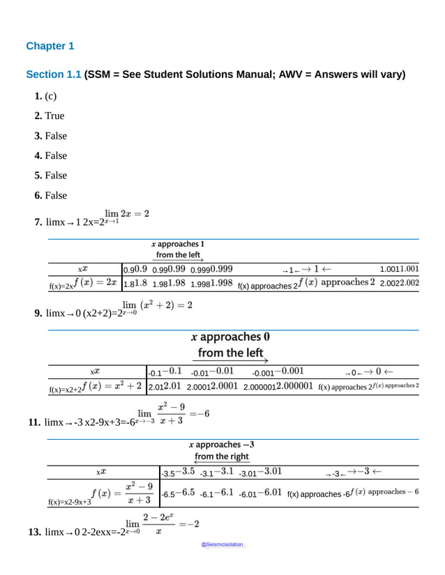
7. limx→1 2x
x 0.9 0.99 0.999 →1← 1.001 1.01 1.1
f(x)=2x
8. limx→2 (x+3)
x 1.9 1.99 1.999 →2← 2.001 2.01 2.1
@Seismicisolation
@Seismicisolation

263. f(x)=x+3
9. limx→0 (x2+2)
x −0.1 −0.01 −0.001 →0← 0.001 0.01
f(x)=x2+2
10. limx→−1 (x2−2)
x −1.1 −1.01 −1.001 →−1← −0.999
f(x)=x2−2
11. limx→−3 x2−9x+3
x −3.5 −3.1 −3.01 → −3 ← −2.99
f(x)=x2−9x+3
12. limx→−1 x3+1x+1
x −1.1 −1.01 −1.001 →−1← −0.999
f(x)=x3+1x+1
In Problems 13–16, use technology to complete the table and investigate the limit.
13. limx→0 2−2exx
@Seismicisolation
@Seismicisolation

264. x −0.2 −0.1 −0.01 →0← 0.01 0.1 0.2
f(x)=2−2exx
14. limx→1 ln xx−1
x 0.9 0.99 0.999 →1← 1.001 1.01 1.1
f(x)=ln xx−1
15. limx→0 1−cos xx, where x is measured in radians
x (in radians) −0.2 −0.1 −0.01 →0← 0.01 0.1
f(x)=1−cos xx
16. limx→0 sin x1+tan x, where x is measured in radians
x (in radians) −0.2 −0.1 −0.01 →0← 0.01 0.1
f(x)=sin x1+tan x
In Problems 17–20, use the graph to investigate (a) limx→2− f(x) (b)
limx→2+ f(x) (c) limx→2 f(x) .
17.
@Seismicisolation
@Seismicisolation

265. 18.
The
value
of
f
is
increasing
from
x
less
than
2
and
decreasing
for
x
greater
19.
20.
@Seismicisolation
@Seismicisolation

266. In Problems 21–28, use the graph to investigate limx→c f(x) . If the limit does not
exist, explain why.
21.
22.
23.
@Seismicisolation
@Seismicisolation

267. 24.
25.
26.
@Seismicisolation
@Seismicisolation

268. 27.
28.
In Problems 29–36, use a graph to investigate limx→c f(x) at the number c.
@Seismicisolation
@Seismicisolation

269. 29. f(x)=2x+5 if x≤24x+1 if x>2 at c=2
30. f(x)=2x+1 if x≤02x if x>0 at c=0
31. f(x)=3x−1if x<14if x=14x if x>1 at c=1
32. f(x)=x+2 if x<24 if x=2x2 if x>2 at c=2
33. f(x)=2x2 if x<13x2−1 if x>1 at c=1
34. f(x)=x3 if x<−1x2−1 if x>−1 at c=−1
35. f(x)=x2 if x≤02x+1 if x>0 at c=0
36. f(x)=x2 if x<12 if x=1−3x+2 if x>1 at c=1
Applications and Extensions
In Problems 37–40, sketch a graph of a function with the given properties. Answers will vary.
@Seismicisolation
@Seismicisolation

270. 37. limx→2 f(x)=3; limx→3− f(x)=3; limx→3+ f(x)=1;
f(2)=3; f(3)=1
38. limx→−1 f(x)=0; limx→2− f(x)=−2;
limx→2+ f(x)=−2; f(−1) is not defined; f(2)=−2
39. limx→1 f(x)=4; limx→0− f(x)=−1;
limx→0+ f(x)=0; f(0)=−1; f(1)=2
40. limx→2 f(x)=2; limx→−1 f(x)=0; limx→1 f(x)=1;
f(−1)=1; f(2)=3
In Problems 41–50, use either a graph or a table to investigate each limit.
41. limx→5+ |x−5|x−5
42. limx→5− |x−5|x−5
43. limx→12− ⌊2x⌋
44. limx→12+ ⌊2x⌋
45. limx→23− ⌊2x⌋
46. limx→23+ ⌊2x⌋
47. limx→2+ |x|−x
48. limx→2− |x|−x
49. limx→2+ ⌊x⌋−x3
@Seismicisolation
@Seismicisolation

271. 50. limx→2− ⌊x⌋−x3
51. Slope of a Tangent Line For f(x)=3x2 :
a. Find the slope of the secant line containing the points (2,12) and (3,27).
b. Find the slope of the secant line containing the points (2,12) and (x,f(x)),
x≠2.
c. Create a table to investigate the slope of the tangent line to the graph of f at 2
using the result from (b).
d. On the same set of axes, graph f, the tangent line to the graph of f at the point
(2,12), and the secant line from (a).
52. Slope of a Tangent Line For f(x)=x3 :
a. Find the slope of the secant line containing the points (2,8) and (3,27).
b. Find the slope of the secant line containing the points (2,8) and (x,f(x)),
x≠2.
c. Create a table to investigate the slope of the tangent line to the graph of f at 2
using the result from (b).
d. On the same set of axes, graph f, the tangent line to the graph of f at the point
(2,8), and the secant line from (a).
53. Slope of a Tangent Line For f(x)=12 x2−1 :
a. Find the slope msec of the secant line containing the points P=(2,f(2))
and Q=(2+h,f(2+h)).
b. Use the result from (a) to complete the following table:
h −0.5 −0.1 −0.001 0.001 0.1 0.5
msec
c. Investigate the limit of the slope of the secant line found in (a) as h→0.
d. What is the slope of the tangent line to the graph of f at the point P=(2,f(2))
?
e. On the same set of axes, graph f and the tangent line to f at P=(2,f(2)).
@Seismicisolation
@Seismicisolation

272. 54. Slope of a Tangent Line For f(x)=x2−1 :
a. Find the slope msec of the secant line containing the points P=(−1,f(−1))
and Q=(−1+h,f(−1+h)).
b. Use the result from (a) to complete the following table:
h −0.1 −0.01 −0.001 −0.0001 0.0001 0.001
msec
c. Investigate the limit of the slope of the secant line found in (a) as h→0.
d. What is the slope of the tangent line to the graph of f at the point P=(−1,f(−1))
?
e. On the same set of axes, graph f and the tangent line to f at P=(−1,f(−1)).
55.
a. Investigate limx→0 cos πx by using a table and evaluating the function
f(x)=cos πx at x=−12,−14,−18,−110, −112,
…,112,110,18,14,12.
b. Investigate limx→0 cos πx by using a table and evaluating the function
f(x)=cos πx at x=−1,−13,−15,−17,−19,…,19,17,15,13,1.
c. Compare the results from (a) and (b). What do you conclude about the limit? Why do
you think this happens? What is your view about using a table to draw a conclusion
about limits?
d. Use technology to graph f. Begin with the x -window [−2π,2π] and the
y -window [−1,1]. If you were finding limx→0 f(x) using a
graph, what would you conclude? Zoom in on the graph. Describe what you see.
(Hint: Be sure your calculator is set to the radian mode.)
56.
a. Investigate limx→0 cos πx2 by using a table and evaluating the function
f(x)=cos πx2 at x=−0.1, −0.01, −0.001,
−0.0001,…,0.0001, 0.001, 0.01, 0.1.
@Seismicisolation
@Seismicisolation

273. b. Investigate limx→0 cos πx2 by using a table and evaluating the function
f(x)=cos πx2 at x=−23, −25, −27, −29,…,29,27,
25, 23.
c. Compare the results from (a) and (b). What do you conclude about the limit? Why do
you think this happens? What is your view about using a table to draw a conclusion
about limits?
d. Use technology to graph f. Begin with the x -window −2π,2π and the y
-window [−1,1]. If you were finding limx→0 f(x) using a graph,
what would you conclude? Zoom in on the graph. Describe what you see.
(Hint: Be sure your calculator is set to the radian mode.)
57.
a. Use a table to investigate limx→2 x−82.
b. How close must x be to 2, so that f(x) is within 0.1 of the limit?
c. How close must x be to 2, so that f(x) is within 0.01 of the limit?
58.
a. Use a table to investigate limx→2 (5−2x).
b. How close must x be to 2, so that f(x) is within 0.1 of the limit?
c. How close must x be to 2, so that f(x) is within 0.01 of the limit?
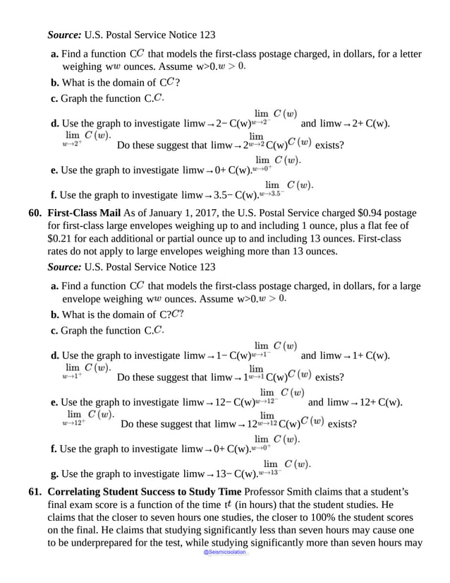
59. First-Class Mail As of January 1, 2017, the U.S. Postal Service charged $0.47 postage
for first-class letters weighing up to and including 1 ounce, plus a flat fee of $0.21 for
each additional or partial ounce up to and including 3.5 ounces. First-class letter rates do
not apply to letters weighing more than 3.5 ounces.
@Seismicisolation
@Seismicisolation

274. Source: U.S. Postal Service Notice 123
a. Find a function C that models the first-class postage charged, in dollars, for a letter
weighing w ounces. Assume w>0.
b. What is the domain of C ?
c. Graph the function C.
d. Use the graph to investigate limw→2− C(w) and limw→2+ C(w).
Do these suggest that limw→2 C(w) exists?
e. Use the graph to investigate limw→0+ C(w).
f. Use the graph to investigate limw→3.5− C(w).
60. First-Class Mail As of January 1, 2017, the U.S. Postal Service charged $0.94 postage
for first-class large envelopes weighing up to and including 1 ounce, plus a flat fee of
$0.21 for each additional or partial ounce up to and including 13 ounces. First-class
rates do not apply to large envelopes weighing more than 13 ounces.
Source: U.S. Postal Service Notice 123
a. Find a function C that models the first-class postage charged, in dollars, for a large
envelope weighing w ounces. Assume w>0.
b. What is the domain of C?
c. Graph the function C.
d. Use the graph to investigate limw→1− C(w) and limw→1+ C(w).
Do these suggest that limw→1 C(w) exists?
e. Use the graph to investigate limw→12− C(w) and limw→12+ C(w).
Do these suggest that limw→12 C(w) exists?
f. Use the graph to investigate limw→0+ C(w).
g. Use the graph to investigate limw→13− C(w).
61. Correlating Student Success to Study Time Professor Smith claims that a student’s
final exam score is a function of the time t (in hours) that the student studies. He
claims that the closer to seven hours one studies, the closer to 100% the student scores
on the final. He claims that studying significantly less than seven hours may cause one
to be underprepared for the test, while studying significantly more than seven hours may
@Seismicisolation
@Seismicisolation

275. cause “burnout.”
a. Write Professor Smith’s claim symbolically as a limit.
b. Write Professor Smith’s claim using the ε -δ definition of limit.
Source: Submitted by the students of Millikin University.
62. The definition of the slope of the tangent line to the graph of y=f(x) at the
point (c,f(c)) is mtan=limx→c f(x)−f(c)x−c. Another
way to express this slope is to define a new variable h=x−c. Rewrite the
slope of the tangent line mtan using h and c.
63. If f(2)=6, can you conclude anything about limx→2 f(x)? Explain
your reasoning.
64. If limx→2 f(x)=6, can you conclude anything about f(2)? Explain
your reasoning.
65. The graph of f(x)=x−33−x is a straight line with a point punched out.
a. What straight line and what point?
b. Use the graph of f to investigate the one-sided limits of f as x approaches 3.
c. Does the graph suggest that limx→3 f(x) exists? If so, what is it?
66.
a. Use a table to investigate limx→0 (1+x)1⁄x.
b. Use graphing technology to graph g(x)=(1+x)1⁄x.
c. What do (a) and (b) suggest about limx→0 (1+x)1⁄x?
d. Find limx→0 (1+x)1⁄x.
Challenge Problems
For Problems 67–70, investigate each of the following limits.
f(x)=1 if x is an integer0 if x is not an integer
67. limx→2 f(x)
@Seismicisolation
@Seismicisolation

276. 68. limx→1⁄2 f(x)
69. limx→3 f(x)
70. limx→0 f(x)
1. = NOW WORK problem
= Graphing technology recommended
= Computer Algebra System recommended
@Seismicisolation
@Seismicisolation

277. (1)
1.2 Limits of Functions Using Properties of Limits
OBJECTIVE When you finish this section, you should be able to:
1 Find the limit of a sum, a difference, and a product
2 Find the limit of a power and the limit of a root
3 Find the limit of a polynomial
4 Find the limit of a quotient
5 Find the limit of an average rate of change
6 Find the limit of a difference quotient
In Section 1.1, we used a numerical approach (tables) and a graphical approach to investigate
limits. We saw that these approaches are not always reliable. The only way to be sure a limit
is correct is to use the ε–δ definition of a limit. In this section, we state without proof
results based on the ε–δ definition. Some of the results are proved in Section 1.6 and
others in Appendix B.
We begin with two basic limits.
THEOREM The Limit of a Constant
If f(x)=A, where A is a constant, then for any real number c,
limx→cf(x)=limx→cA=A
The theorem is proved in Section 1.6. See Figure 17 and Table 8 for graphical and
numerical support of limx→c A=A.
@Seismicisolation
@Seismicisolation

278. (2)
Figure 17 For x close to c, the value of f remains at A; limx→c A=A.
TABLE 8
x c−0.01 c−0.001 c−0.0001 → c ← c+0.0001 c+0.001
f(x)=A A A A f(x)
remains at A
A
For example,
limx→5 2=2limx→2 13=13limx→5(−π)=−π
THEOREM The Limit of the Identity Function
If f(x)=x, then for any real number c,
limx→c f (x)=limx→c x=c
This theorem is proved in Section 1.6. See Figure 18 and Table 9 for graphical and
numerical support of limx→c x=c.
@Seismicisolation
@Seismicisolation

279. Figure 18 For x close to c, the value of f is just as close to c; limx→c x=c.
TABLE 9
x c−0.01 c−0.001 c−0.0001 → c ← c+0.0001 c+0.001
f(x)=x c−0.01 c−0.001 c−0.0001 f(x)
approaches c
c+0.0001 c+0.001
For example,
limx→−5 x=−5limx→3 x=3limx→0 x=0
1 Find the Limit of a Sum, a Difference, and a Product
Many functions are combinations of sums, differences, and products of a constant function
and the identity function. The following properties can be used to find the limit of such
functions.
THEOREM Limit of a Sum
If f and g are functions for which limx→c f(x) and limx→c g(x) both
exist, then limx→c [f(x)+g(x)] exists and
limx→c [f(x)+g(x)]=limx→c f(x)+limx→c g(x)
@Seismicisolation
@Seismicisolation

280. IN WORDS The limit of the sum of two functions equals the sum of their limits.
A proof is given in Appendix B.
EXAMPLE 1 Finding the Limit of a Sum
Find limx→−3 (x+4).
Solution F(x)=x+4 is the sum of two functions f(x)=x and g(x)=4.
From the limits given in (1) and (2), we have
limx→−3 f(x)=limx→−3 x=−3andlimx→−3 g(x)=limx→−34=4
Then using the Limit of a Sum, we have
limx→−3 (x+4)=limx→−3 x+limx→−34=−3+4=1
▪
THEOREM Limit of a Difference
If f and g are functions for which limx→c f (x) and limx→c g (x) both
exist, then limx→c [f (x)−g (x)] exists and
limx→c [f (x)−g (x)]=limx→c f (x)−limx→c g (x)
IN WORDS The limit of the difference of two functions equals the difference of their limits.
EXAMPLE 2 Finding the Limit of a Difference
Find limx→4 (6−x).
Solution F (x)=6−x is the difference of two functions f (x)=6 and
g (x)=x.
@Seismicisolation
@Seismicisolation

281. limx→4 f (x)=limx→4 6=6andlimx→4 g (x)=limx→4 x=4
Then using the Limit of a Difference, we have
limx→4 (6−x)=limx→4 6−limx→4 x=6−4=2
▪
THEOREM Limit of a Product
If f and g are functions for which limx→c f (x) and limx→c g (x) both
exist, then limx→c [f (x)⋅g (x)] exists and
limx→c [f (x)⋅g (x)]=limx→c f (x)⋅limx→c g (x)
IN WORDS The limit of the product of two functions equals the product of their limits.
A proof is given in Appendix B.
EXAMPLE 3 Finding the Limit of a Product
Find:
a. limx→3 x2
b. limx→−5 (−4x)
Solution a. F(x)=x2 is the product of two functions, f(x)=x and
g(x)=x. Then using the Limit of a Product, we have
limx→3 x2=limx→3 x⋅limx→3 x=3⋅3=9
b. F(x)=−4x is the product of two functions, f(x)=−4 and g(x)=x.
Then using the Limit of a Product, we have
limx→−5 (−4x)=limx→−5(−4)⋅limx→−5 x=(−4)(−5)=20
@Seismicisolation
@Seismicisolation

282. ▪
A corollary* of the Limit of a Product Theorem is the special case when f(x)=k
is a constant function.
COROLLARY Limit of a Constant Times a Function
If g is a function for which limx→c g(x) exists and if k is any real number, then
limx→c [kg(x)] exists and
limx→c [kg(x)]=k limx→c g(x)
IN WORDS The limit of a constant times a function equals the constant times the limit of the function.
You are asked to prove this corollary in Problem 103.
Limit properties often are used in combination.
EXAMPLE 4 Finding a Limit
Find:
a. limx→1 [2x(x+4)]
b. limx→2+ [4x(2−x)]
Solution a.
limx→1 [(2x)(x+4)]=limx→1(2x)limx→1(x+4)Limit of a
Product=2⋅limx→1 x⋅limx→1 x+limx→1 4Limit of a Constant Times a Function, Limit of a
Sum=(2⋅1)⋅(1+4)=10Use (2) and (1), and simplify.
b. We use properties of limits to find the one-sided limit.
limx→2+ [4x(2−x)]=4limx→2+ [x(2−x)]=4limx→2+ xlimx→2+
(2−x)=4⋅2limx→2+2−limx→2+ x=4⋅2⋅(2−2)=0
@Seismicisolation
@Seismicisolation

283. ▪
NOTE The limit properties are also true for one-sided limits.
NOW WORK Problem 13.
To find the limit of piecewise-defined functions at numbers where the defining equation
changes requires the use of one-sided limits.
EXAMPLE 5 Finding a Limit for a Piecewise-defined Function
Find limx→2 f(x), if it exists.
f(x)=3x+1ifx<22x(x−1)ifx≥2
Solution Since the rule for f changes at 2, we need to find the one-sided limits of f as
x approaches 2.
For x<2, we use the left-hand limit. Also, because x<2, f(x)=3x+1.
limx→2− f(x)=limx→2−(3x+1)=limx→2−(3x)+limx→2−1=3limx→2− x+1=3⋅2+1=7
For x≥2, we use the right-hand limit. Also, because x≥2, f(x)=2x(x−1).
limx→2+ f(x)=limx→2+ [2x(x−1)]=limx→2+(2x)⋅limx→2+(x−1)=2limx→2+ x⋅limx→2+ x
−limx→2+1=2⋅2[2−1]=4
Since limx→2− f(x)=7≠limx→2+ f(x)=4, limx→2 f(x)
@Seismicisolation
@Seismicisolation

284. does not exist. ▪
See Figure 19.
Figure 19 f(x)=3x+1 ifx<22x(x−1)ifx≥2
RECALL The limit L of a function y=f(x) as x approaches a number c exists if and only if
limx→c− f(x)=limx→c+ f(x)=L.
NOW WORK Problem 73.
The Heaviside function, uc(t)=0ift<c1ift≥c, is a function that is
used in electrical engineering to model a switch. The switch is off if t<c, and it is on if
t≥c.
@Seismicisolation
@Seismicisolation

285. ORIGINS Oliver Heaviside (1850-1925) was a self-taught mathematician and electrical engineer. He
developed a branch of mathematics called operational calculus in which differential equations are solved by
converting them to algebraic equations. Heaviside applied vector calculus to electrical engineering and,
perhaps most significantly, he simplified Maxwell’s equations to the form used by electrical engineers to this
day. In 1902 Heaviside claimed there is a layer surrounding Earth from which radio signals bounce, allowing the
signals to travel around the Earth. Heaviside’s claim was proved true in 1923. The layer, contained in the
ionosphere, is named the Heaviside layer. The function we discuss here is one of his minor contributions to
mathematics and electrical engineering.
EXAMPLE 6 Finding a Limit of the Heaviside Function
Find limt→0 u0(t), where u0(t)=0ift<01ift≥0
Solution Since the Heaviside function changes rules at t=0, we find the one-sided
limits as t approaches 0.
For t<0,limt→0− u0(t)=limt→0−0=0andfor t≥0,limt→0+u0(t)=limt→0+1=1
Since the one-sided limits as t approaches 0 are not equal, limt→0 u0(t) does
not exist. ▪
NOW WORK Problem 81.
2 Find the Limit of a Power and the Limit of a Root
Using the Limit of a Product, if limx→c f(x) exists, then
@Seismicisolation
@Seismicisolation

286. limx→c [f(x)]2=limx→c [f(x)⋅f(x)]=limx→c f(x)⋅limx→c f(x)=[limx→c f(x)]2
Repeated use of this property produces the next corollary.
COROLLARY Limit of a Power
If limx→c f(x) exists and if n is a positive integer, then
limx→c [f(x)]n= [limx→c f(x)]n
EXAMPLE 7 Finding the Limit of a Power
Find:
a. limx→2 x5
b. limx→1 (2x−3)3
c. limx→c xn n a positive integer
Solution a. limx→2 x5=limx→2 x5=25=32
b. limx→1 (2x−3)3=limx→1 (2x−3)3=limx→1 (2x)−limx→1 33=(2−3)3=−1
c. limx→c xn=limx→c xn=cn ▪
The result from Example 7(c) is worth remembering since it is used frequently:
limx→c xn=cn
where c is a number and n is a positive integer.
NOW WORK Problem 15.
THEOREM Limit of a Root
@Seismicisolation
@Seismicisolation

287. If limx→c f(x) exists and if n≥2 is an integer, then
limx→c f(x)n=limx→c f(x)n
provided f(x)>0 if n is even.
EXAMPLE 8 Finding the Limit of a Root
Find limx→4 x2+113.
Solution
▪
NOW WORK Problem 19.
The Limit of a Power and the Limit of a Root are used together to find the limit of a
function with a rational exponent.
THEOREM Limit of a Fractional Power [f(x)]m⁄n
If f is a function for which limx→c f(x) exists and if [f(x)]m⁄n is
defined for positive integers m and n, then
limx→c [f(x)]m⁄n=limx→c f(x)m⁄n
EXAMPLE 9 Finding the Limit of a Fractional Power [f(x)]m⁄n
Find limx→8 (x+1)3⁄2.
@Seismicisolation
@Seismicisolation

288. Solution Let f(x)=x+1. Near 8, x+1>0, so (x+1)3⁄2 is
defined. Then
▪
See Figure 20.
Figure 20 f(x)=(x+1)3⁄2
NOW WORK Problem 23.
3 Find the Limit of a Polynomial
Sometimes limx→c f(x) can be found by substituting c for x in f(x). For
example,
limx→2 (5x2)=5 limx→2 x2=5⋅22=20
Since limx→c xn=cn if n is a positive integer, we can use the Limit of a
Constant Times a Function to obtain a formula for the limit of a monomial f(x)=axn.
limx→c (axn)=acn
@Seismicisolation
@Seismicisolation

289. where a is any number.
Since a polynomial is the sum of monomials and the limit of a sum is the sum of the
limits, we have the following result.
THEOREM Limit of a Polynomial Function
If P is a polynomial function, then
limx→c P(x)=P(c)
for any number c.
Proof If P is a polynomial function, that is, if
P(x)=anxn+an−1xn−1+⋯+a1x+a0
where n is a nonnegative integer, then
limx→c P(x)=limx→c anxn+an−1xn−1+⋯+a1x+a0=limx→c anxn+limx→c an−1xn−1+⋯
+limx→c (a1x)+limx→c a0=ancn+an−1cn−1+⋯+a1c+a0Limit of a Monomial=P(c)
▪
IN WORDS To find the limit of a polynomial as x approaches c, evaluate the polynomial at c.
EXAMPLE 10 Finding the Limit of a Polynomial
Find the limit of each polynomial:
a. limx→3 (4x2−x+2)=4⋅32−3+2=35
b. limx→−1 (7x5+4x3−2x2)=7(−1)5+4(−1)3−2(−1)2=−13
c. limx→0 (10x6−4x5−8x+5)=10⋅06−4⋅05−8⋅0+5=5
@Seismicisolation
@Seismicisolation

290. (3)
▪
NOW WORK Problem 29.
4 Find the Limit of a Quotient
To find the limit of a rational function, which is the quotient of two polynomials, we use the
following result.
THEOREM Limit of a Quotient
If f and g are functions for which limx→c f(x) and limx→c g(x) both
exist, then limx→c f(x)g(x) exists and
limx→c f(x)g(x)=limx→c f(x)limx→c g(x)
provided limx→c g(x)≠0.
IN WORDS The limit of the quotient of two functions equals the quotient of their limits, provided that the limit of
the denominator is not zero.
COROLLARY Limit of a Rational Function
If the number c is in the domain of a rational function R(x)=p(x)q(x), then
limx→c R(x)=R(c)
NEED TO REVIEW? Rational functions are discussed in Section P.2, p. 22.
You are asked to prove this corollary in Problem 104.
EXAMPLE 11 Finding the Limit of a Rational Function
@Seismicisolation
@Seismicisolation

291. Find:
a. limx→1 3x3−2x+14x2+5
b. limx→−2 2x+43x2−1
Solution a. Since 1 is in the domain of the rational function R(x)=3x3−2x+14x2+5,
b. Since −2 is in the domain of the rational function H(x)=2x+43x2−1,
▪
NOW WORK Problem 33.
EXAMPLE 12 Finding the Limit of a Quotient
Find limx→4 3x2+1x−1.
Solution We seek the limit of the quotient of two functions. Since the limit of the
denominator limx→4 (x−1)≠0, we use the Limit of a Quotient.
▪
NOW WORK Problem 31.
@Seismicisolation
@Seismicisolation

292. Based on these examples, you might be tempted to conclude that finding a limit as x
approaches c is simply a matter of substituting the number c into the function. The next
few examples show that substitution cannot always be used and other strategies need to be
employed.
The limit as x approaches c of a rational function can be found using substitution,
provided the number c is in the domain of the rational function. The next example shows a
strategy that can be tried when c is not in the domain.
EXAMPLE 13 Finding the Limit of a Rational Function
Find limx→−2 x2+5x+6x2−4.
Solution Since −2 is not in the domain of the rational function, substitution cannot be
used. But this does not mean that the limit does not exist! Factoring the numerator and the
denominator, we find
x2+5x+6x2−4=(x+2)(x+3)(x+2)(x−2)
Since x≠−2, and we are interested in the limit as x approaches −2, the factor
x+2 can be divided out. Then
▪
NOW WORK Problem 35.
The Limit of a Quotient property can be used only when the limit of the denominator of
the function is not zero. The next example illustrates a strategy to try if radicals are present.
EXAMPLE 14 Finding the Limit of a Quotient
Find limx→5 x−5x−5.
Solution The domain of h(x)=x−5x−5 is x|x≥0,x≠5.
@Seismicisolation
@Seismicisolation

293. Since the limit of the denominator is
limx→5 (x−5)=0
we cannot use the Limit of a Quotient property. A different strategy is necessary. We
rationalize the numerator of the quotient.
Do you see why rationalizing the numerator works? It causes the term x−5 to appear in
the numerator, and since x≠5, the factor x−5 can be divided out. Then
▪
NOTE When finding a limit, remember to include “limx→c ” at each step until you let x→c.
NOW WORK Problem 41.
5 Find the Limit of an Average Rate of Change
The next two examples illustrate limits that we encounter in Chapter 2.
If c and x, where x≠c, are in the domain of a function y=f(x), the
average rate of change of f from c to x is
ΔyΔx=f(x)−f(c)x−cx≠c
NEED TO REVIEW? Average rate of change is discussed in Section P.1, p. 12.
EXAMPLE 15 Finding the Limit of an Average Rate of Change
a. Find the average rate of change of f(x)=x2+3x from 2 to x, x≠2.
b. Find the limit as x approaches 2 of the average rate of change of f(x)=x2+3x
@Seismicisolation
@Seismicisolation

294. from 2 to x.
Solution a. The average rate of change of f from 2 to x is
ΔyΔx=f(x)−f(2)x−2=(x2+3x)−[22+3⋅2]x−2=x2+3x−10x−2=(x+5)(x−2)x−2
b. The limit of the average rate of change is
limx→2 f(x)−f(2)x−2=limx→2 (x+5)(x−2)x−2=limx→2 (x+5)=7
▪
NOW WORK Problem 63.
6 Find the Limit of a Difference Quotient
In Section P.1, we defined the difference quotient of a function f at x as
f(x+h)−f(x)hh≠0
EXAMPLE 16 Finding the Limit of a Difference Quotient
a. For f(x)=2x2−3x+1, find the difference quotient f(x+h)
−f(x)h, h≠0.
b. Find the limit as h approaches 0 of the difference quotient of f(x)=2x2−3x+1.
Solution a. To find the difference quotient of f, we begin with f(x+h).
f(x+h)=2(x+h)2−3(x+h)+1=2(x2+2xh+h2)−3x−3h+1=2x2+4xh+2h2−3x−3h+1
Now
f(x+h)−f(x)=(2x2+4xh+2h2−3x−3h+1)−(2x2−3x+1)=4xh+2h2−3h
@Seismicisolation
@Seismicisolation

295. Then the difference quotient is
f(x+h)−f(x)h=4xh+2h2−3hh=h(4x+2h−3)h=4x+2h−3, h≠0
b. limh→0 f(x+h)−f(x)h=limh→0(4x+2h−3)=4x+0−3=4x−3
▪
NOW WORK Problem 69.
Summary
Two Basic Limits
limx→c A=A, where A is a constant.
limx→c x=c
Properties of Limits
If f and g are functions for which limx→c f(x) and limx→c g(x) both
exist, and k is a constant, then
Limit of a Sum or a Difference: limx→c [f(x)±g(x)]=limx→c f(x)±limx→c g(x)
Limit of a Product: limx→c [f(x)⋅g(x)]=limx→c f(x)⋅limx→c g(x)
Limit of a Constant Times a Function: limx→c [kg(x)]=k limx→c g(x)
Limit of a Power: limx→c [f(x)]n=limx→c f(x)n where n is
a positive integer
Limit of a Root: limx→c f(x)n=limx→c f(x)n where n≥2
is an integer, provided f(x)>0 if n is even
Limit of [f(x)]m⁄n : limx→c [f(x)]m⁄n=limx→c f(x)m⁄n
@Seismicisolation
@Seismicisolation

296. provided [f(x)]m⁄n is defined for positive
integers m and n
Limit of a Quotient: limx→c f(x)g(x)=limx→c f(x)limx→c g(x)
provided limx→c g(x)≠0
Limit of a Polynomial Function: limx→c P(x)=P(c)
Limit of a Rational Function: limx→c R(x)=R(c) if c is in the
domain of R
1.2 Assess Your Understanding
Concepts and Vocabulary
1. a. limx→4 (−3)=_______________;
b. limx→0 π=_______________
2. If limx→c f(x)=3, then limx→c[f(x)]5=_______________.
3. If limx→c f(x)=64, then limx→cf(x)3=_______________.
4. a. limx→−1 x=_______________;
b. limx→e x=_______________
5. a. limx→0 (x−2)=_______________;
b. limx→1⁄2 (3+x)=_______________
6. a. limx→2 (−3x)=_______________;
b. limx→0 (3x)=_______________
7. True or False If p is a polynomial function, then limx→5 p(x)=p(5).
@Seismicisolation
@Seismicisolation

297. 8. If the domain of a rational function R is {x|x≠0}, then
limx→2 R(x)=R(________).
9. True or False Properties of limits cannot be used for one-sided limits.
10. True or False If f(x)=(x+1)(x+2)x+1 and g(x)=x+2,
then limx→−1 f(x)=limx→−1 g(x).
Skill Building
In Problems 11–44, find each limit using properties of limits.
11. limx→3 [2(x+4)]
12. limx→−2 [3(x+1)]
13. limx→−2 [x(3x−1)(x+2)]
14. limx→−1 [x(x−1)(x+10)]
15. limt→1 (3t−2)3
16. limx→0 (−3x+1)2
17. limx→4 (3x)
18. limx→8 14x3
19. limx→3 5x−4
20. limt→2 3t+4
21. limt→2 [t(5t+3)(t+4)]
22. limt→−1 [t(t+1)(2t−1)3]
@Seismicisolation
@Seismicisolation

298. 23. limx→9 x+x+41⁄2
24. limt→2 t2t+41⁄3
25. limt→−1 [4t(t+1)]2⁄3
26. limx→0 (x2−2x)3⁄5
27. limt→1 (3t2−2t+4)
28. limx→0 (−3x4+2x+1)
29. limx→12 (2x4−8x3+4x−5)
30. limx→−13 (27x3+9x+1)
31. limx→4 x2+4x
32. limx→3 x2+53x
33. limx→−2 2x3+5x3x−2
34. limx→1 2x4−13x3+2
35. limx→2 x2−4x−2
36. limx→−2 x+2x2−4
37. limx→−1 x3−xx+1
38. limx→−1 x3+x2x2−1
@Seismicisolation
@Seismicisolation

299. 39. limx→−8 2xx+8+16x+8
40. limx→2 3xx−2−6x−2
41. limx→2 x−2x−2
42. limx→3 x−3x−3
43. limx→4 x+5−3(x−4)(x+1)
44. limx→3 x+1−2x(x−3)
In Problems 45–50, find each one-sided limit using properties of limits.
45. limx→3− (x2−4)
46. limx→2+ (3x2+x)
47. limx→3− x2−9x−3
48. limx→3+ x2−9x−3
49. limx→3− 9−x2+x2
50. limx→2+ 2x2−4+3x
In Problems 51–58, use the information below to find each limit.
limx→c f(x)=5limx→c g(x)=2limx→c h(x)=0
51. limx→c [f(x)−3g(x)]
52. limx→c [5f(x)]
@Seismicisolation
@Seismicisolation

300. 53. limx→c [g(x)]3
54. limx→c f(x)g(x)−h(x)
55. limx→c h(x)g(x)
56. limx→c [4f(x)⋅g(x)]
57. limx→c 1g(x)2
58. limx→c 5g(x)−33
In Problems 59 and 60, use the graphs of the functions and properties of limits to find each
limit, if it exists. If the limit does not exist, write, “The limit does not exist,” and explain why.
59.
a. limx→4 f (x)+g(x)
b. limx→4 f (x)g(x)−h(x)
c. limx→4 [f (x)⋅g(x)]
d. limx→4 [2h(x)]
e. limx→4 g(x)f (x)
f. limx→4 h(x)f (x)
@Seismicisolation
@Seismicisolation

301. Line
depicting
h
of
x
contains
points
(3,
minus
2)
and
(4,
0).
F
of
x
curve
is
discontinuous
at
x
equal
to
4.
At
x
60.
a. limx→3 2f(x)+h(x)
b. limx→3− [g(x)+h(x)]
c. limx→3 h(x)3
d. limx→3 f(x)h(x)
e. limx→3 [h(x)]3
f. limx→3 [f(x)−2h(x)]3⁄2
@Seismicisolation
@Seismicisolation

302. Line
depicting
h
of
x
contains
points
(3,
minus
2)
and
(0,
2).
f
of
x
has
a
minimum
value
at
(3,
0).
g
of
In Problems 61–66, for each function f, find the limit as x approaches c of the average
rate of change of f from c to x . That is, find
limx→c f(x)−f(c)x−c
61. f(x)=3x2,c=1
62. f(x)=8x3,c=2
63. f(x)=−2x2+4,c=1
64. f(x)=20−0.8x2,c=3
65. f(x)=x,c=1
66. f(x)=2x,c=5
In Problems 67–72, find the limit of the difference quotient for each function f . That is, find
limh→0 f(x+h)−f(x)h.
67. f(x)=4x−3
68. f(x)=3x+5
69. f(x)=3x2+4x+1
@Seismicisolation
@Seismicisolation

303. 70. f(x)=2x2+x
71. f(x)=2x
72. f(x)=3x2
In Problems 73–80, find limx→c− f(x) and limx→c+ f(x) for the given
number c. Based on the results, determine whether limx→c f(x) exists.
73. f(x)=2x−3 if x≤13−x if x>1 at c=1
74. f(x)=5x+2 if x<21+3x if x≥2 at c=2
75. f(x)=3x−1 if x<14 if x=12x if x>1 at c=1
76. f(x)=3x−1 if x<12 if x=12x if x>1 at c=1
77. f(x)=x−1 if x<1x−1 if x>1 at c=1
78. f(x)=9−x2 if 0<x<3x2−9 if x>3 at c=3
@Seismicisolation
@Seismicisolation

304. 79. f(x)=x2−9x−3 if x≠36 if x=3 at c=3
80. f(x)=x−2x2−4 if x≠21 if x=2 at c=2
Applications and Extensions
Heaviside Functions In Problems 81 and 82, find the limit, if it exists, of the given Heaviside
function at c.
81. u1(t)=0 if t<11 if t≥1 at c=1
82. u3(t)=0 if t<31 if t≥3 at c=3
In Problems 83–92, find each limit.
83. limh→0 (x+h)2−x2h
84. limh→0 x+h−xh
85. limh→0 1x+h−1xh
86. limh→0 1(x+h)3−1x3h
87. limx→0 1x 14+x−14
88. limx→−1 2x+1 13−1x+4 @Seismicisolation
@Seismicisolation

305. 89. limx→7 x−7x+2−3
90. limx→2 x−2x+2−2
91. limx→1 x3−3x2+3x−1x2−2x+1
92. limx→−3 x3+7x2+15x+9x2+6x+9
93. Cost of Water The Jericho Water District determines quarterly water costs, in dollars,
using the following rate schedule:
Water used (in
thousands of gallons)
Cost
0≤x≤10 $9.00
10<x≤30
$9.00+0.95 for each thousand gallons in
excess of 10,000 gallons
30<x≤100
$28.00+1.65 for each thousand gallons in
excess of 30,000 gallons
x>100
$143.50+2.20 for each thousand gallons in
excess of 100,000 gallons
Source: Jericho Water District, Syosset, NY.
a. Find a function C that models the quarterly cost, in dollars, of using x thousand
gallons of water.
b. What is the domain of the function C?
c. Find each of the following limits. If the limit does not exist, explain why.
limx→5 C(x) limx→10 C(x) limx→30 C(x) limx→100 C(x)
d. What is limx→0+ C(x)?
e. Graph the function C.
94. Cost of Electricity In December 2016, Florida Power and Light had the following
monthly rate schedule for electric usage in single-family residences:
Monthly customer
charge $7.87
Fuel charge
@Seismicisolation
@Seismicisolation

306. ≤1000
kWH
$0.02173 per kWH
>1000
kWH
$21.73+0.03173 for each kWH in excess of
1000
Source: Florida Power and Light, Miami, FL.
a. Find a function C that models the monthly cost, in dollars, of using x kWH of
electricity.
b. What is the domain of the function C?
c. Find limx→1000 C(x), if it exists. If the limit does not exist, explain
why.
d. What is limx→0+ C(x)?
e. Graph the function C.
95. Low-Temperature Physics In thermodynamics, the average molecular kinetic energy
(energy of motion) of a gas having molecules of mass m is directly proportional to its
temperature T on the absolute (or Kelvin) scale. This can be expressed as
12 mv2=32 kT, where v=v(T) is the speed of a typical
molecule at time t and k is a constant, known as the Boltzmann constant.
a. What limit does the molecular speed v approach as the gas temperature T
approaches absolute zero (0 K or −273 ∘C or −469 ∘F )?
b. What does this limit suggest about the behavior of a gas as its temperature
approaches absolute zero?
96. For the function f(x)=3x+5ifx≤213−xifx>2, find
a. limh→0− f(2+h)−f(2)h
b. limh→0+ f(2+h)−f(2)h
c. Does limh→0 f(2+h)−f(2)h exist?
97. Use the fact that | x|=x if x≥0−x if x<0 to show that limx→0|x|=0.
@Seismicisolation
@Seismicisolation

307. 98. Use the fact that | x|=x2 to show that limx→0|x|=0.
99. Find functions f and g for which limx→c [f(x)+g(x)] may exist
even though limx→c f(x) and limx→c g(x) do not exist.
100. Find functions f and g for which limx→c [f(x)g(x)] may exist even
though limx→c f(x) and limx→c g(x) do not exist.
101. Find functions f and g for which limx→c f(x)g(x) may exist even though
limx→c f(x) and limx→c g(x) do not exist.
102. Find a function f for which limx→c |f(x)| may exist even though
limx→c f(x) does not exist.
103. Prove that if g is a function for which limx→c g(x) exists and if k is any
real number, then limx→c [kg(x)] exists and
limx→c [kg(x)]=klimx→c g(x).
104. Prove that if the number c is in the domain of a rational function R(x)=
p(x)q(x), then limx→c R(x)=R(c).
Challenge Problems
105. Find limx→a xn−anx−a, n a positive integer.
106. Find limx→−a xn+anx+a, n a positive integer.
107. Find limx→1 xm−1xn−1, m, n positive integers.
108. Find limx→0 1+x3−1x.
109. Find limx→0 (1+ax)(1+bx)−1x.
@Seismicisolation
@Seismicisolation

308. 110. Find limx→0 (1+a1 x)(1+a2 x)⋯(1+an x)−1x.
111. Find limh→0 f(h)−f(0)h if f(x)=x|x|.
1. = NOW WORK problem
= Graphing technology recommended
= Computer Algebra System recommended
* A corollary is a theorem that follows directly from a previously proved theorem.
@Seismicisolation
@Seismicisolation

309. 1.3 Continuity
OBJECTIVES When you finish this section, you should be able to:
1 Determine whether a function is continuous at a number
2 Determine intervals on which a function is continuous
3 Use properties of continuity
4 Use the Intermediate Value Theorem
Sometimes limx→c f(x) equals f(c) and sometimes it does not. In fact, f(c)
may not even be defined and yet limx→c f(x) may exist. In this section, we
investigate the relationship between limx→c f(x) and f(c). Figure 21 shows
some possibilities.
Figure 21
In
the
first
figure,
left
hand
limit
of
f
of
x,
right
hand
Of these five graphs, the “nicest” one is Figure 21(a). There, limx→c f(x) exists
and is equal to f(c). Functions that have this property are said to be continuous at the
number c. This agrees with the intuitive notion that a function is continuous if its graph
can be drawn without lifting the pencil. The functions in Figures 21(b)–(e) are not continuous
at c, since each has a break in the graph at c. This leads to the definition of continuity at
a number.
DEFINITION Continuity at a Number
A function f is continuous at a number c if the following three conditions are met:
f(c) is defined (that is, c is in the domain of f )
limx→c f(x) exists
@Seismicisolation
@Seismicisolation

310. limx→c f(x)=f(c)
If a function f is defined on an open interval containing c, except possibly at c, then
the function is discontinuous at c, whenever any one of the above three conditions is not
satisfied.
1 Determine Whether a Function Is Continuous at a Number
EXAMPLE 1 Determining Whether a Function Is Continuous at a Number
a. Determine whether f(x)=3x2−5x+4 is continuous at 1.
b. Determine whether g(x)=x2+9x2−4 is continuous at 2.
Solution a. We begin by checking the conditions for continuity. First, 1 is in the domain of
f and f(1)=2. Second, limx→1 f(x)=limx→1(3x2−5x+4)=2,
so limx→1 f(x) exists. Third,
limx→1 f(x)=f(1). Since the three conditions are met, f is continuous at 1.
b. Since 2 is not in the domain of g, the function g is discontinuous at 2.
▪
Figure 22 shows the graphs of f and g from Example 1. Notice that f is continuous at
1, and its graph is drawn without lifting the pencil. But the function g is discontinuous at
2, and to draw its graph, you must lift your pencil at x=2.
@Seismicisolation
@Seismicisolation

311. Figure 22
NOW WORK Problem 19.
EXAMPLE 2 Determining Whether a Function Is Continuous at a Number
Determine whether f(x)=x2+2x2−4 is continuous at the numbers −2,0,
and 2.
Solution The domain of f is {x|x≠−2, x≠2}. Since f is not defined at
−2 and 2, the function f is not continuous at −2 and at 2. The number 0 is in
the domain of f. That is, f is defined at 0, and f(0)=−24. Also,
limx→0 f(x)= limx→0 x2+2x2−4=limx→0x2+2limx→0(x2−4)=limx→0(x2+2)limx→0 x2−lim
−24=f(0)
The three conditions of continuity at a number are met. So, the function f is continuous at 0.
▪
Figure 23 shows the graph of f.
@Seismicisolation
@Seismicisolation

312. Figure 23 f is continuous at 0 ; f is discontinuous at −2 and 2 .
NOW WORK Problem 21.
EXAMPLE 3 Determining Whether a Piecewise-Defined Function Is Continuous
Determine whether the function
f(x)=x2−9x−3 if x<39 if x=3x2−3 if x>3
is continuous at 3.
Solution Since f(3)=9, the function f is defined at 3. To check the second
condition, we investigate the one-sided limits.
@Seismicisolation
@Seismicisolation

313. Since limx→3− f(x)=limx→3+ f(x), then limx→3 f(x)
exists. But, limx→3 f(x)=6 and f(3)=9, so the third condition of
continuity is not satisfied. The function f is discontinuous at 3.
▪
Figure 24 shows the graph of f.
Figure 24 f is discontinuous at 3.
NOW WORK Problem 25.
The discontinuity at c=3 in Example 3 is called a removable discontinuity because
we can redefine f at the number c to equal limx→c f(x) and make f continuous
at c. So, in Example 3, if f(3) is redefined to be 6, then f would be continuous at
3.
DEFINITION Removable Discontinuity
Let f be a function that is defined everywhere in an open interval containing c, except
possibly at c. The number c is called a removable discontinuity of f if the function is
discontinuous at c but limx→c f(x) exists. The discontinuity is removed by
defining (or redefining) the value of f at c to be limx→c f(x).
@Seismicisolation
@Seismicisolation

314. IN WORDS Visually, the graph of a function f with a removable discontinuity has a hole at (c,limx→c f (x)).
The discontinuity is removable because we can fill in the hole by appropriately defining f.
The function will then be continuous at x=c.
NOW WORK Problems 13 and 35.
EXAMPLE 4 Determining Whether a Function Is Continuous at a Number
Determine whether the floor function f(x)=⌊x⌋ is continuous at 1.
NEED TO REVIEW? The floor function is discussed in Section P.2, p.19.
Solution The floor function f(x)=⌊x⌋=the greatest integer≤x.
The floor function f is defined at 1 and f(1)=1.
But
limx→1− f(x)=limx→1−⌊x⌋=0 and limx→1+ f(x)=limx→1+⌊x⌋=1
So, limx→1 ⌊x⌋ does not exist. Since limx→1⌊x⌋ does not exist, f is
discontinuous at 1.
Figure 25 illustrates that the floor function is discontinuous at each integer. Also, none of
the discontinuities of the floor function is removable. Since at each integer the value of the
floor function “jumps” to the next integer, without taking on any intermediate values, the
discontinuity at integer values is called a jump discontinuity.
@Seismicisolation
@Seismicisolation

315. Figure 25 f(x)=⌊x⌋
NOW WORK Problem 53.
We have defined what it means for a function f to be continuous at a number. Now we
define one-sided continuity at a number.
DEFINITION One-Sided Continuity at a Number
Let f be a function defined on the interval (a,c]. Then f is continuous from the
left at the number c if
limx→c− f(x)=f(c)
Let f be a function defined on the interval [c,b). Then f is continuous from the
right at the number c if
limx→c+ f(x)=f(c)
In Example 4, we showed that the floor function f(x)=⌊x⌋ is discontinuous at
x=1. But since
f(1)=⌊1⌋=1 and limx→1+ f(x)=⌊x⌋=1
the floor function is continuous from the right at 1. In fact, the floor function is
discontinuous at each integer n, but it is continuous from the right at every integer n.
(Do you see why?)
@Seismicisolation
@Seismicisolation

316. 2 Determine Intervals on Which a Function Is Continuous
So far, we have considered only continuity at a number c. Now we use one-sided
continuity to define continuity on an interval.
DEFINITION Continuity on an Interval
A function f is continuous on an open interval (a,b) if f is continuous at
every number in (a,b).
A function f is continuous on an interval [a,b) if f is continuous on the open
interval (a,b) and continuous from the right at the number a.
A function f is continuous on an interval (a,b] if f is continuous on the open
interval (a,b) and continuous from the left at the number b.
A function f is continuous on a closed interval a,b if f is continuous on the
open interval (a,b), continuous from the right at a, and continuous from the left
at b.
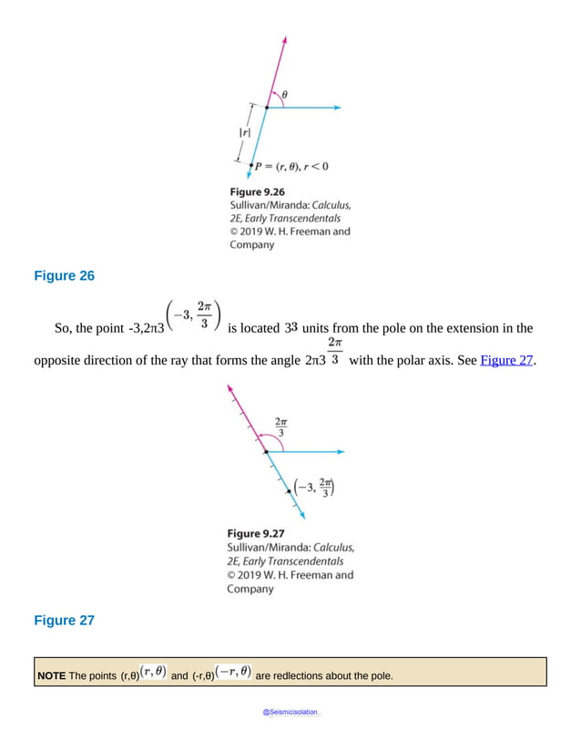
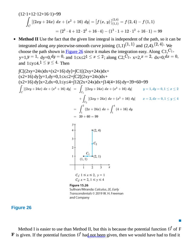
Figure 26 gives examples of graphs over different types of intervals.
Figure 26
In
the
first
figure,
f
is
continuous
on
the
open
interval
For example, the graph of the floor function f(x)=⌊x⌋ in Figure 25 illustrates
that f is continuous on every interval [n,n+1), n an integer. In each interval, f
is continuous from the right at the left endpoint n and is continuous at every number in the
open interval (n,n+1).
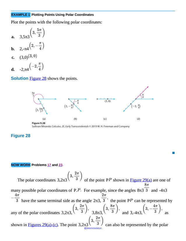
EXAMPLE 5 Determining Whether a Function Is Continuous on a Closed Interval
Is the function f(x)=4−x2 continuous on the closed interval [−2,2] ?
Solution The domain of f is {x|−2≤x≤2}. So, f is defined for every
@Seismicisolation
@Seismicisolation

317. number in the closed interval [−2,2].
For any number c in the open interval (−2,2),
limx→c f(x)=limx→c 4−x2=limx→c (4−x2)=4−c2=f(c)
So, f is continuous on the open interval (−2,2).
To determine whether f is continuous on [−2,2], we investigate the limit from
the right at −2 and the limit from the left at 2. Then
limx→−2+ f(x)=limx→−2+4−x2=0=f(−2)
So, f is continuous from the right at −2. Similarly,
limx→2− f(x)=limx→2−4−x2=0=f(2)
So, f is continuous from the left at 2. We conclude that f is continuous on the closed
interval [−2,2].
▪
Figure 27 shows the graph of f.
Figure 27 f(x)=4−x2,−2≤x≤2
NOW WORK Problems 37 and 77.
EXAMPLE 6 Determining Where f(x)=x2x−1 Is Continuous
@Seismicisolation
@Seismicisolation

318. Determine where the function f(x)=x2x−1 is continuous.
Solution The domain of f(x)=x2x−1 is the set {x|x≠1}, which is
the same as the set (−∞,1)∪(1,∞).
Since f is not defined at the number 1, f is discontinuous at 1.
We examine f on the intervals (−∞,1) and (1,∞).
For all numbers c in the open interval (−∞,1) we have f(c)=c2c−1,
and
limx→c x2x−1=limx→c x2limx→c (x−1)=c2c−1=f(c)
So, f is continuous on the open interval (−∞,1).
For all numbers c in the open interval (1,∞), we have f(c)=c2c−1,
and
limx→c x2x−1=limx→c x2limx→c (x−1)=c2c−1=f(c)
So, f is continuous on the open interval (1,∞).
The function f(x)=x2x−1 is continuous on (−∞,1)∪(1,∞).
▪
Figure 28 shows the graph of f.
@Seismicisolation
@Seismicisolation

319. Figure 28 f(x)=x2x−1 is continuous on (−∞,1)∪(1,∞).
When listing the properties of a function in Chapter P, we included the function’s
domain, its symmetry, and its zeros. Now we add continuity to the list by asking, “Where is
the function continuous?” We answer this question here for two important classes of
functions: polynomial functions and rational functions.
THEOREM
A polynomial function is continuous on its domain, all real numbers.
A rational function is continuous on its domain.
Proof If P is a polynomial function, its domain is the set of real numbers. For a
polynomial function,
limx→c P(x)=P(c)
for any number c. That is, a polynomial function is continuous at every real number.
If R(x)=p(x)q(x) is a rational function, then p(x) and q(x) are
polynomials and the domain of R is {x|q(x)≠0}. The Limit of a Rational
Function (p. 96) states that for all c in the domain of a rational function,
limx→c R(x)=R(c)
@Seismicisolation
@Seismicisolation

320. So a rational function is continuous at every number in its domain. ▪
Rational functions deserve special attention. For example, the rational function
R(x)=x2−2x+1x−1 is continuous for {x|x≠1}. But notice in
Figure 29 that its graph has a hole at (1,0). The rational function f(x)=1x is
continuous for {x|x≠0}. But notice in Figure 30 the behavior of the graph as x
goes from negative numbers to positive numbers.
Figure 29 The graph of R has a hole at (1,0).
@Seismicisolation
@Seismicisolation

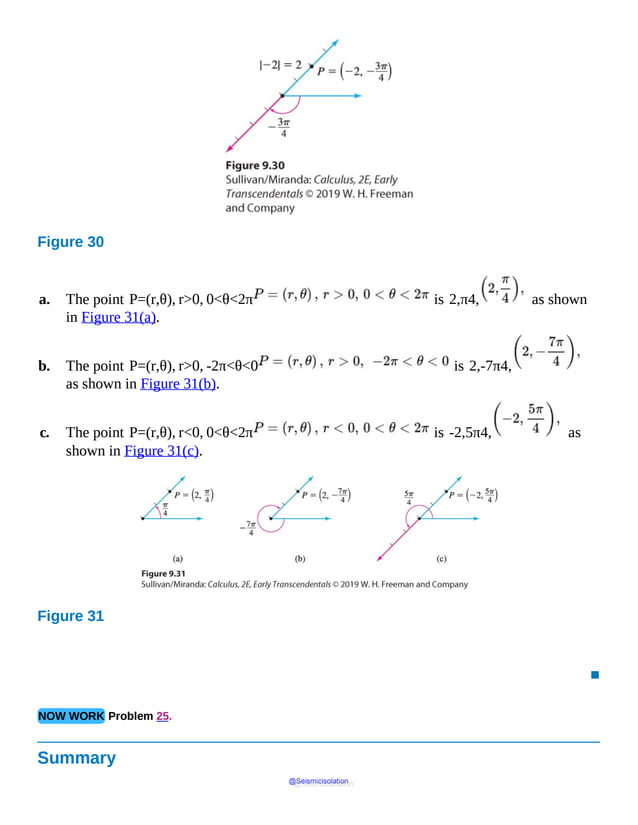
321. Figure 30 f is not defined at 0.
3 Use Properties of Continuity
Once we know where functions are continuous, we can build other continuous functions.
THEOREM Continuity of a Sum, Difference, Product, and Quotient
If the functions f and g are continuous at a number c, and if k is a real number, then
the functions f+g, f−g, f⋅g, and kf are also continuous at c. If g(c)≠0,
the function fg is continuous at c.
The proofs of these properties are based on properties of limits. For example, the proof of
the continuity of f+g is based on the Limit of a Sum property. That is, if limx→c f(x)
and limx→c g(x) exist, then
limx→c [f(x)+g(x)]=limx→c f(x)+limx→c g(x).
EXAMPLE 7 Identifying Where Functions Are Continuous
Determine where each function is continuous:
a. F(x)=x2+5−xx2+4
@Seismicisolation
@Seismicisolation

322. b. G(x)=x3+2x+x2x2−1
Solution
a. F is the difference of the two functions f(x)=x2+5 and g(x)=xx2+4,
each of which is contionuous for all real numbers. The function F=f−g
is also continuous for all real numbers.
b. G is the sum of the two functions f(x)=x3+2x, which is continuous for
all real numbers, and g(x)=x2x2−1, which is continuous for x|x≠−1,x≠−1.
Since G=f+g, G is continuous for, x|x≠−1,x≠1.
▪
NOW WORK Problem 45.
The continuity of a composite function depends on the continuity of its components.
NEED TO REVIEW? Composite functions are discussed in Section P.3, pp. 27–30.
THEOREM Continuity of a Composite Function
If a function g is continuous at c and a function f is continuous at g(c), then the
composite function (f∘g)(x)=f(g(x)) is continuous at c. That is,
limx→c (f∘g)(x)=limx→c f(g(x))=f[limx→c g(x)]=f(g(c))
EXAMPLE 8 Identifying Where Functions Are Continuous
Determine where each function is continuous:
a. F(x)=x2+4
b. G(x)=x2−1
@Seismicisolation
@Seismicisolation

323. c. H(x)=x2−1x2−4+x−1
Solution a. F=f∘g is the composite of f(x)=x and g(x)=x2+4
; f is continuous for x≥0 ; and g is continuous for all real numbers.
The function F=(f∘g)(x)=x2+4 is also continuous for all real
numbers.
b. G is the composite of f(x)=x and g(x)=x2−1 ; f is continuous
for x≥0 ; and g is continuous for all real numbers. The function G=(f∘g)(x)=x2−1
is continuous for x2−1≥0, the set {x|x≤−1}∪{x|x≥1}.
c. H is the sum of f(x)=x2−1x2−4 and the function g(x)=x−1;
f is continuous on {x|x≠−⁢2,x≠2} ; and g is continuous
on {x|x≥1}. The function H is continuous on [1,2)∪(2,∞).
▪
NOW WORK Problem 47.
Recall that for any function f that is one-to-one over its domain, its inverse f−1 is
also a function, and the graphs of f and f−1 are symmetric with respect to the line y=x.
It is intuitive that if f is continuous, then so is f−1. See Figure 31. The
following theorem, whose proof is given in Appendix B, confirms this.
@Seismicisolation
@Seismicisolation

324. Figure 31
NEED TO REVIEW? Inverse functions are discussed in Section P.4, pp. 37–40.
THEOREM Continuity of an Inverse Function
If f is a one-to-one function that is continuous on its domain, then its inverse function f−1
is also continuous on its domain.
4 Use the Intermediate Value Theorem
Functions that are continuous on a closed interval have many important properties. One of
them is stated in the Intermediate Value Theorem. The proof of the Intermediate Value
Theorem may be found in most books on advanced calculus.
THEOREM The Intermediate Value Theorem
Let f be a function that is continuous on a closed interval [a,b] and f(a)≠f(b).
If N is any number between f(a) and f(b), then there is at least
one number c in the open interval (a,b) for which f(c)=N.
To get a better idea of this result, suppose you climb a mountain, starting at an elevation
of 2000 meters and ending at an elevation of 5000 meters. No matter how many
ups and downs you take as you climb, at some time your altitude must be 3765.6
meters, or any other number between 2000 and 5000.
@Seismicisolation
@Seismicisolation

325. In other words, a function f that is continuous on a closed interval [a,b] with
f(a)≠f(b), must take on all values between f(a) and f(b). Figure 32
illustrates this. Figure 33 shows why the continuity of the function is crucial. Notice in
Figure 33 that there is a hole in the graph of f at the point (c,N ). Because of the
discontinuity at c, there is no number c in the open interval (a,b ) for which f(c)=N.
Figure 32 f takes on every value between f(a) and f(b).
@Seismicisolation
@Seismicisolation

326. Figure 33 The discontinuity at c results in no number c in (a,b) for which f(c)=N.
The Intermediate Value Theorem is an existence theorem. It states that there is at least
one number c for which f(c)=N, but it does not tell us how to find c. However,
we can use the Intermediate Value Theorem to locate an open interval (a,b ) that contains
c.
An immediate application of the Intermediate Value Theorem involves locating the zeros
of a function. Suppose a function f is continuous on the closed interval [a,b] and f(a)
and f(b) have opposite signs. Then by the Intermediate Value Theorem, there is at
least one number c between a and b for which f(c)=0. That is, f has at least
one zero between a and b.
EXAMPLE 9 Using the Intermediate Value Theorem
Use the Intermediate Value Theorem to show that
f(x)=x3+x2−x−2
has a zero between 1 and 2.
Solution Since f is a polynomial, it is continuous on the closed interval [1,2].
Because f(1)=−1 and f(2)=8 have opposite signs, the Intermediate Value
Theorem states that f(c)=0 for at least one number c in the interval (1,2).
That is, f has at least one zero between 1 and 2. Figure 34 shows the graph of f on a
@Seismicisolation
@Seismicisolation

327. graphing calculator.
Figure 34 f(x)=x3+x2−x−2
NOW WORK Problem 59.
The Intermediate Value Theorem can be used to approximate a zero in the interval (a,b)
by dividing the interval [a,b] into smaller subintervals. There are two popular
methods of subdividing the interval [a,b].
The bisection method bisects [a,b], that is, divides [a,b] into two equal
subintervals and compares the sign of fa+b2 to the signs of the previously
computed values f(a) and f(b). The subinterval whose endpoints have opposite
signs is then bisected, and the process is repeated.
The second method divides [a,b] into 10 subintervals of equal length and
compares the signs of f evaluated at each of the 11 endpoints. The subinterval whose
endpoints have opposite signs is then divided into 10 subintervals of equal length and
the process is repeated.
We choose to use the second method because it lends itself well to the table feature of a
graphing calculator. You are asked to use the bisection method in Problems 107–114.
EXAMPLE 10 Using the Intermediate Value Theorem to Approximate a Real Zero of a Function
The function f(x)=x3+x2−x−2 has a zero in the interval (1,2).
Use the Intermediate Value Theorem to approximate the zero correct to three decimal places.
@Seismicisolation
@Seismicisolation

328. Solution Using the TABLE feature on a graphing utility, subdivide the interval [1,2]
into 10 subintervals, each of length 0.1. Then find the subinterval whose endpoints
have opposite signs, or the endpoint whose value equals 0 (in which case, the exact zero is
found). From Figure 35, since f(1.2)=−0.032 and f(1.3)=0.587,
by the Intermediate Value Theorem, a zero lies in the interval (1.2,1.3).
Correct to one decimal place, the zero is 1.2.
@Seismicisolation
@Seismicisolation

329. @Seismicisolation
@Seismicisolation

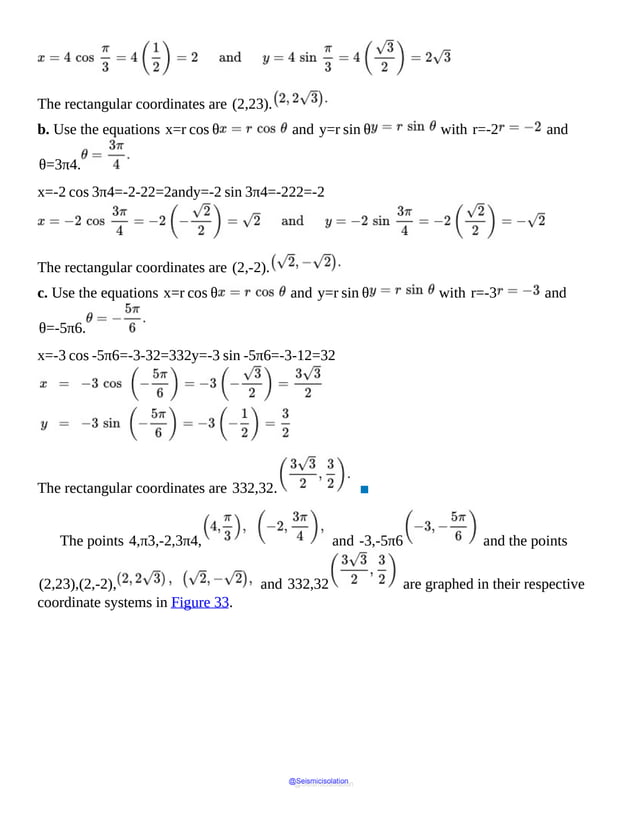
330. Figure 35
Repeat the process by subdividing the interval [1.2,1.3] into 10 subintervals,
each of length 0.01. See Figure 36. We conclude that the zero is in the interval
(1.20,1.21), so correct to two decimal places, the zero is 1.20.
Figure 36
Now subdivide the interval 1.20,1.21 into 10 subintervals, each of length
0.001. See Figure 37.
Figure 37
We conclude that the zero of the function f is 1.205, correct to three decimal
places.
▪
Notice that a benefit of the method used in Example 10 is that each additional iteration
results in one additional decimal place of accuracy for the approximation.
NOW WORK Problem 65.
1.3 Assess Your Understanding
Concepts and Vocabulary
@Seismicisolation
@Seismicisolation

331. 1. True or False A polynomial function is continuous at every real number.
2. True or False Piecewise-defined functionsare never continuous at numbers where the
function changes equations.
3. The three conditions necessary for a function f to be continuous at a number c are
_____________, _____________, and _____________.
4. True or False If f is continuous at 0, then g(x)=14 f(x) is
continuous at 0.
5. True or False If f is a function defined everywhere in an open interval containing c,
except possibly at c, then the number c is called a removable discontinuity of f if
the function f is not continuous at c.
6. True or False If a function f is discontinuous at a number c, then limx→c f(x)
does not exist.
7. True or False If a function f is continuous on an open interval (a,b), then it is
continuous on the closed interval [a,b].
8. True or False If a function f is continuous on the closed interval [a,b], then f
is continuous on the open interval (a,b).
In Problems 9 and 10, explain whether each function is continuous or discontinuous.
9. The velocity of a ball thrown up into the air as a function of time, if the ball lands 5
seconds after it is thrown and stops.
10. The temperature of an oven used to bake a potato as a function of time.
11. True or False If a function f is continuous on a closed interval [a,b], and
f(a)≠f(b), then the Intermediate Value Theorem guarantees that the
function takes on every value between f(a) and f(b).
12. True or False If a function f is continuous on a closed interval [a,b] and
f(a)≠f(b), but both f(a)>0 and f(b)>0, then according to
the Intermediate Value Theorem, f does not have a zero on the open interval (a,b).
Skill Building
In Problems 13–18, use the graph of y=f(x) (below).
a. Determine whether f is continuous at c.
@Seismicisolation
@Seismicisolation

332. b. If f is discontinuous at c, state which condition(s) of the definition of continuity is
(are) not satisfied.
c. If f is discontinuous at c, determine if the discontinuity is removable.
d. If the discontinuity is removable, define (or redefine) f at c to make f continuous at
c.
13. c=−3
14. c=0
15. c=2
16. c=3
17. c=4
18. c=5
In Problems 19–32, determine whether the function f is continuous at c .
19. f(x)=x2+1 at c=−1
20. f(x)=x3−5 at c=5
21. f(x)=xx2+4 at c=−2
22. f(x)=xx−2 at c=2
23. f(x)=2x+5 if x≤24x+1 if x>2 at c=2
@Seismicisolation
@Seismicisolation

333. 24. f(x)=2x+1 if x≤02x if x>0 at c=0
25. f(x)=3x−1 if x<14 if x=12x if x>1 at c=1
26. f(x)=3x−1 if x<1 2 if x=1 at c=12x if x>1
27. f(x)=3x−1 if x<12x if x>1 at c=1
28. f(x)=3x−1 if x<12 if x=1 at c=13x if x>1
29. f(x)=x2 if x≤02x if x>0 at c=0
30. f(x)=x2 if x<−12 if x=−1−3x+2 if x>−1 at c=−1
@Seismicisolation
@Seismicisolation

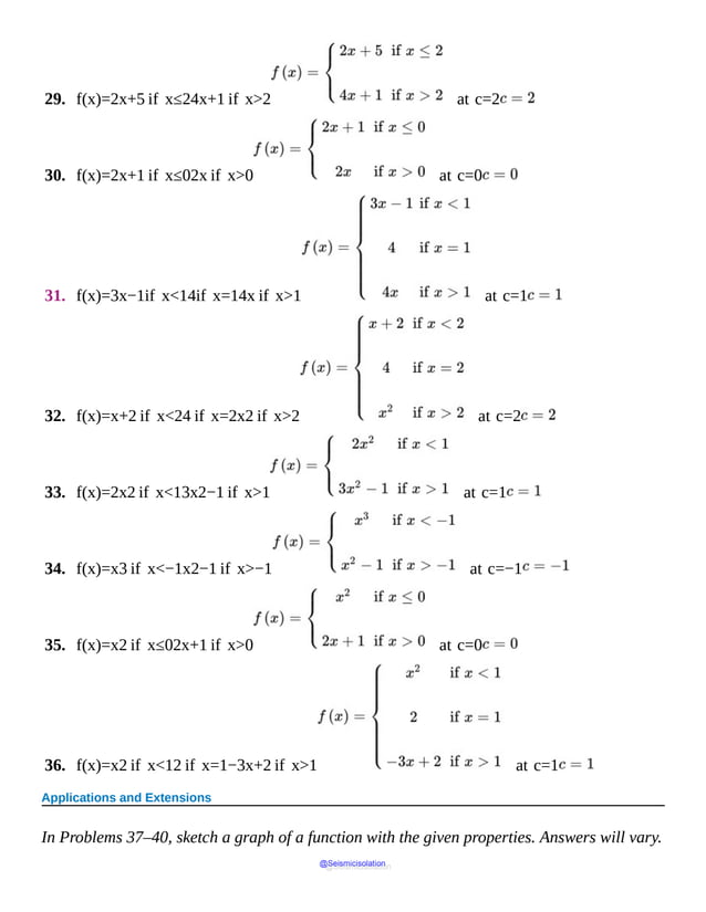
334. 31. f(x)=4−3x2 if x<04 if x=016−x24−x if 0<x<4 at c=0
32. f(x)=4+x if−4≤x≤4x2−3x−4x−4 if x>4 at
c=4
In Problems 33–36, each function f has a removable discontinuity at c. Define f(c)
so that f is continuous at c .
33. f(x)=x2−4x−2, c=2
34. f(x)=x2+x−12x−3, c=3
35. f(x)=1+x if x<14 if x=12x if x>1 c=1
36. f(x)=x2+5x if x< −10 if x= −1x −3 if x> −1 c=−1
In Problems 37–40, determine whether each function f is continuous on the given interval.
If the answer is no, find the numbers in the interval, if any, at which f is continuous.
37. f(x)=x2−9x−3 on the interval [−3,3]
@Seismicisolation
@Seismicisolation

335. 38. f(x)=1+1x on the interval [−1,0]
39. f(x)=1x2−9 on the interval [−3,3]
40. f(x)=9−x2 on the interval [−3,3]
In Problems 41–50, determine where each function f is continuous by using properties of
continuity.
41. f(x)=2x2+5x−1x
42. f(x)=x+1+2xx2+5
43. f(x)=(x−1)(x2+x+1)
44. f(x)=x(x3−5)
45. f(x)=x−9x−3
46. f(x)=x−4x−2
47. f(x)=x2+12−x
48. f(x)=4x2−1
49. f(x)=(2x2+5x−3)2⁄3
50. f(x)=(x+2)1⁄2
In Problems 51–56, use the function
@Seismicisolation
@Seismicisolation

336. f(x)=15−3x if x<25 if x=29−x2 if 2<x<3⌊x−2⌋ if 3≤x
51. Is f continuous at 0 ? Why or why not?
52. Is f continuous at 4 ? Why or why not?
53. Is f continuous at 3 ? Why or why not?
54. Is f continuous at 2 ? Why or why not?
55. Is f continuous at 1 ? Why or why not?
56. Is f continuous at 2.5 ? Why or why not?
In Problems 57 and 58:
a. Use technology to graph f using a suitable scale on each axis.
b. Based on the graph from (a), determine where f is continuous.
c. Use the definition of continuity to determine where f is continuous.
d. What advice would you give a fellow student about using technology to determine
where a function is continuous?
57. f(x)=x3−8x−2
58. f(x)=x2−3x+23x−6
In Problems 59–64, use the Intermediate Value Theorem to determine which of the functions
must have zeros in the given interval. Indicate those for which the theorem gives no
information. Do not attempt to locate the zeros.
59. f(x)=x3−3x on [−2,2]
60. f(x)=x4−1 on [−2,2]
61. f(x)=x(x+1)2−1 on [10,20]
@Seismicisolation
@Seismicisolation

337. 62. f(x)=x3−2x2−x+2 on [3,4]
63. f(x)=x3−1x−1 on [0,2]
64. f(x)=x2+3x+2x2−1 on [−3,0]
In Problems 65–72, verify that each function has a zero in the indicated interval. Then
use the Intermediate Value Theorem to approximate the zero correct to three decimal places
by repeatedly subdividing the interval containing the zero into 10 subintervals.
65. f(x)=x3+3x−5 ; interval: [1,2]
66. f(x)=x3−4x+2 ; interval: [1,2]
67. f(x)=2x3+3x2+4x−1 ; interval: [0,1]
68. f(x)=x3−x2−2x+1 ; interval: [0,1]
69. f(x)=x3−6x−12 ; interval: [3,4]
70. f(x)=3x3+5x−40 ; interval: [2,3]
71. f(x)=x4−2x3+21x−23 ; interval: [1,2]
72. f(x)=x4−x3+x−2 ; interval: [1,2]
In Problems 73 and 74,
a. Use the Intermediate Value Theorem to show that f has a zero in the given interval.
b. Use technology to find the zero rounded to three decimal places.
73. f(x)=x2+4x−2 in [0,1]
74. f(x)=x3−x+2 in [−2,0]
Applications and Extensions
In Problems 75–78, determine whether each function is
a. continuous from the left
b. continuous from the right at the numbers c and d.
75. f(x)=x2 if −1<x<1x−1 if| x|≥1 at c=−1 and d=1
@Seismicisolation
@Seismicisolation

338. 76. f(x)=x2−1 if −1≤x≤1|x+1| if| x|>1 at c=−1 and d=1
77. f(x)=(x+1)(x−5) at c=−1 and d=5
78. f(x)=(x−1)(x−2) at c=1 and d=2
79. First-Class Mail As of January 1, 2017, the U.S. Postal Service charged $0.47 postage
for first-class letters weighing up to and including 1 ounce, plus a flat fee of $0.21 for
each additional orpartial ounce up to 3.5 ounces. First-class letter rates do not apply to
letters weighing more than 3.5 ounces.
Source: U.S. Postal Service Notice 123.
a. Find a function C that models the first-class postage charged for a letter weighing
ω ounces. Assume ω>0.
b. What is the domain of C?
c. Determine the intervals on which C is continuous.
d. At numbers where C is not continuous (if any), what type of discontinuity does C
have?
e. What are the practical implications of the answer to (d)?
80. First-Class Mail As of January 1, 2017, the U.S. Postal Service charged $0.94 postage
for first-class large envelopes weighing up to and including 1 ounce, plus a flat fee of
$0.21 for each additional or partial ounce up to 13 ounces. First-class rates do not apply
to large envelopes weighing more than 13 ounces.
Source: U.S. Postal Service Notice 123.
a. Find a function C that models the first-class postage charged for a large envelope
weighing ω ounces. Assume ω>0.
b. What is the domain of C?
c. Determine the intervals on which C is continuous.
d. At numbers where C is not continuous (if any), what type of discontinuity does C
have?
e. What are the practical implications of the answer to (d)?
81. Cost of Electricity In December 2016, Florida Power and Light had the following
monthly rate schedule for electric usage in single-family residences:
@Seismicisolation
@Seismicisolation

339. Monthly customer charge $7.87
Fuel charge
≤1000 kWH 0.02173 per kWH
>1000 kWH $21.73+0.03173 for each kWH in excess of 1000
Source: Florida Power and Light, Miami, FL.
a. Find a function C that models the monthly cost of using x kWH of electricity.
b. What is the domain of C?
c. Determine the intervals on which C is continuous.
d. At numbers where C is not continuous (if any), what type of discontinuity does C
have?
e. What are the practical implications of the answer to (d)?
82. Cost of Water The Jericho Water District determines quarterly water costs, in dollars,
using the following rate schedule:
Water used
(in thousands of
gallons) Cost
0≤x≤10 $9.00
10<x≤30
$9.00+0.95 for each thousand gallons in excess of 10,000
gallons
30<x≤100
$28.00+1.65 for each thousand gallons in excess of 30,000
gallons
x>100
$143.50+2.20 for each thousand gallons in excess of
100,000 gallons
Source: Jericho Water District, Syosset, NY.
a. Find a function C that models the quarterly cost of using x thousand gallons of
water.
b. What is the domain of C?
c. Determine the intervals on which C is continuous.
d. At numbers where C is not continuous (if any), what type of discontinuity does C
have?
e. What are the practical implications of the answer to (d)?
83. Gravity on Europa Europa, one of the larger satellites of Jupiter, has an icy surface and
appears to have oceans beneath the ice. This makes it a candidate for possible
extraterrestrial life. Because Europa is much smaller than most planets, its gravity is
weaker. If we think of Europa as a sphere with uniform internal density, then inside the
sphere, the gravitational field g is given by
@Seismicisolation
@Seismicisolation

340. g(r)=GmR3 r 0≤r<R
where R is the radius of the sphere, r is the distance from the center of the sphere, and G is the universal
gravitation constant. Outside a uniform sphere of mass m, the gravitational field g is given by
g(r)=Gmr2 R<r
a. For the gravitational field of Europa to be continuous at its surface, what must g(r)
equal?
[Hint: Investigate limr→R g(r) .]
b. Determine the gravitational field at Europa’s surface. This will indicate the type of
gravity environment organisms will experience. Use the following measured
values: Europa’s mass is 4.8×1022 kilograms, its radius is 1.569×106
meters, and G=6.67×10−11.
c. Compare the result found in (b) to the gravitational field on Earth’s surface, which
is 9.8 meter⁄second2. Is the gravity on Europa less than or
greater than that on Earth?
84. Find constants A and B so that the function below is continuous for all x. Graph
the resulting function.
f(x)=(x−1)2if −∞<x<0A−x2if0≤x<1x+Bif1≤x<∞
85. Find constants A and B so that the function below is continuous for all x. Graph
the resulting function.
@Seismicisolation
@Seismicisolation

341. f(x)=x+A if−∞<x<4(x−1)2 if4≤x≤9Bx+1 if9<x<∞
86. For the function f below, find k so that f is continuous at 2.
f(x)=2x+5−x+7x−2 if x≥−52, x≠2k if x=2
87. Suppose f(x)=x2−6x−16(x2−7x−8)x2−4.
a. For what numbers x is f defined?
b. For what numbers x is f discontinuous?
c. Which discontinuities, if any, found in (b) are removable?
88. Intermediate Value Theorem
a. Use the Intermediate Value Theorem to show that the function f(x)=sin x+x−3 has a
zero in the interval [0, π].
b. Approximate the zero rounded to three decimal places.
89. Intermediate Value Theorem
a. Use the Intermediate Value Theorem to show that the function f(x)=ex+x−2 has a zero in
the interval [0, 2].
b. Approximate the zero rounded to three decimal places.
In Problems 90–93, verify that each function intersects the given line in the indicated
interval. Then use the Intermediate Value Theorem to approximate the point of intersection
correct to three decimal places by repeatedly subdividing the interval into 10 subintervals.
90. f(x)=x3−2x2−1; line: y=−1; interval: (1, 4 )
91. g(x)=−x4+3x2+3; line: y=3; interval: (1, 2 )
92. h(x)=x3−5x2+1 ; line: y=1; interval: (1, 3 )
@Seismicisolation
@Seismicisolation

342. 93. r(x)=x−6x2+2 ; line: y=−1; interval: (0, 3 )
94. Graph a function that is continuous on the closed interval [5, 12], that is negative
at both endpoints, and has exactly three distinct zeros in this interval. Does this
contradict the Intermediate Value Theorem? Explain.
95. Graph a function that is continuous on the closed interval [−1, 2], that is
positive at both endpoints, and has exactly two zeros in this interval. Does this
contradict the Intermediate Value Theorem? Explain.
96. Graph a function that is continuous on the closed interval [−2, 3], is positive at
−2 and negative at 3, and has exactly two zeros in this interval. Is this possible?
Does this contradict the Intermediate Value Theorem? Explain.
97. Graph a function that is continuous on the closed interval [−5, 0], is negative at
−5 and positive at 0, and has exactly three zeros in the interval. Is this possible?
Does this contradict the Intermediate Value Theorem? Explain.
98. a. Explain why the Intermediate Value Theorem gives no information about the zeros of the function f(x)=x4−1
on the interval [−2, 2].
b. Use technology to determine whether f has a zero on the interval [−2, 2].
99. a. Explain why the Intermediate Value Theorem gives no information about the zeros of the function f(x)=
ln(x2+2) on the interval [−2, 2].
b. Use technology to determine whether f has a zero on the interval [−2, 2].
100. Intermediate Value Theorem
a. Use the Intermediate Value Theorem to show that the functions y=x3 and y=1−x2 intersect
somewhere between x=0 and x=1.
b. Use technology to find the coordinates of the point of intersection rounded to three
decimal places.
c. Use technology to graph both functions on the same set of axes. Be sure the graph
shows the point of intersection.
101. Intermediate Value Theorem An airplane is traveling at a speed of 620 miles per hour
and then encounters a slight headwind that slows it to 608 miles per hour. After a few
minutes, the headwind eases and the plane’s speed increases to 614 miles per hour.
Explain why the plane’s speed is 610 miles per hour on at least two different occasions
during the flight.
Source: Submitted by the students of Millikin University.
@Seismicisolation
@Seismicisolation

343. 102. Suppose a function f is defined and continuous on the closed interval [a, b]. Is
the function h(x)=1f(x) also continuous on the closed interval [a, b] ?
Discuss the continuity of h on [a, b].
103. Given the two functions f and h :
f(x)=x3−3x2−4x+12h(x)=f(x)x−3 if x≠3p if x=3
a. Find all the zeros of the function f.
b. Find the number p so that the function h is continuous at x=3. Justify
your answer.
c. Determine whether h, with the number found in (b), is even, odd, or neither.
Justify your answer.
104. The function f(x)=|x|x is not defined at 0. Explain why it is impossible to
define f (0) so that f is continuous at 0.
105. Find two functions f and g that are each continuous at c, yet fg is not continuous
at c.
106. Discuss the difference between a discontinuity that is removable and one that is
nonremovable. Give an example of each.
Bisection Method for Approximating Zeros of a Function Suppose the Intermediate Value
Theorem indicates that a function f has a zero in the interval (a,b). The bisection
method approximates the zero by evaluating f at the midpoint m1 of the interval (a,b).
If f(m1)=0, then m1 is the zero we seek and the process ends. If
f(m1)≠0, then the sign of f(m1) is opposite that of either f(a) or f(b)
(but not both), and the zero lies in that subinterval. Evaluate f at the midpoint m2
of this subinterval. Continue bisecting the subinterval containing the zero until the desired
degree of accuracy is obtained.
In Problems 107–114, use the bisection method three times to approximate the zero of each
function in the given interval.
107. f(x)=x3+3x−5 ; interval: [1, 2]
108. f(x)=x3−4x+2 ; interval: [1, 2]
@Seismicisolation
@Seismicisolation

344. 109. f(x)=2x3+3x2+4x−1 ; interval: [0, 1]
110. f(x)=x3,−x2−2x+1 ; interval: [0, 1]
111. f(x)=x3−6x−12 ; interval: [3, 4]
112. f(x)=3x3+5x−40 ; interval: [2, 3]
113. f(x)=x4−2x3+21x−23 ; interval [1, 2]
114. f(x)=x4−x3+x−2 ; interval: [1, 2]
115. Intermediate Value Theorem Use the Intermediate Value Theorem to show that the
function f(x)=x2+4x−2 has a zero in the interval [0, 1].
Then approximate the zero correct to one decimal place.
116. Intermediate Value Theorem Use the Intermediate Value Theorem to show that the
function f(x)=x3−x+2 has a zero in the interval [−2, 0]. Then
approximate the zero correct to two decimal places.
117. Continuity of a Sum If f and g are each continuous at c, prove that f+g is
continuous at c.
(Hint: Use the Limit of a Sum Property.)
118. Intermediate Value Theorem Suppose that the functions f and g are continuous on
the interval [a, b]. If f(a)<g(a) and f(b)>g(b), prove that
the graphs of y=f(x) and y=g(x) intersect somewhere between x=a
and x=b.
[Hint: Define h(x)=f(x)−g(x) and show h(x)=0 for some x
between a and b. ]
Challenge Problems
119. Intermediate Value Theorem Let f(x)=1x−1+1x−2. Use the
Intermediate Value Theorem to prove that there is a real number c between 1 and 2
for which f(c)=0.
120. Intermediate Value Theorem Prove that there is a real number c between 2.64
and 2.65 for which c2=7.
121. Show that the existence of limh→0 f(a+h)−f(a)h implies f is
continuous at x=a.
122. Find constants A, B, C, and D so that the function below is continuous for
all x. Graph the resulting function.
@Seismicisolation
@Seismicisolation

345. f(x)=x2+x−2x−1 if−∞<x<1A ifx=1B x−C2 if1<x<4D ifx=42x−8 if4<x<∞
123. Let f be a function for which 0 ≤f (x)≤1 for all x in [0, 1]. If f is
continuous on [0, 1], show that there exists at least one number c in [0, 1]
such that f(c)=c.
[Hint: Let g(x)=x−f(x). ]
1. = NOW WORK problem
= Graphing technology recommended
= Computer Algebra System recommended
@Seismicisolation
@Seismicisolation

346. 1.4 Limits and Continuity of Trigonometric, Exponential,
and Logarithmic Functions
OBJECTIVES When you finish this section, you should be able to:
1 Use the Squeeze Theorem to find a limit
2 Find limits involving trigonometric functions
3 Determine where the trigonometric functions are continuous
4 Determine where an exponential or a logarithmic function is continuous
Until now we have found limits using the basic limits
limx→c ​​ A=​ A​​ ​​lim x→c​ x=c
and properties of limits. But there are many limit problems that cannot be found by directly
applying these techniques. To find such limits requires different results, such as the Squeeze
Theorem,* or basic limits involving trigonometric and exponential functions.
1 Use the Squeeze Theorem to Find a Limit
To use the Squeeze Theorem to find limx→c g(x), we need to know, or be able to
find, two functions f and h that “sandwich” the function g between them for all x close
to c. That is, in some interval containing c, the functions f, g, and h satisfy the
inequality
f(x)≤g(x)≤h(x)
Then if f and h have the same limit L as x approaches c, the function g is
“squeezed” to the same limit L as x approaches c. See Figure 38.
@Seismicisolation
@Seismicisolation

347. Figure 38
We state the Squeeze Theorem here. The proof is given in Appendix B.
THEOREM Squeeze Theorem
Suppose the functions f, g, and h have the property that for all x in an open interval
containing c, except possibly at c,
f(x)≤g(x)≤h(x)
If
limx→c f(x)=limx→c h(x) = L
then
limx→c g(x)= L
For example, suppose we wish to find limx→0 g(x), and we know that
−x2≤g(x)≤x2
for all x≠0. Since lim x→0 (−x2)=0 and lim x→0x2=0, the
Squeeze Theorem tells us that lim x→0 g(x)=0. Figure 39 illustrates how g is
“squeezed” between y=x2 and y=−x2 near 0.
@Seismicisolation
@Seismicisolation

348. Figure 39
EXAMPLE 1 Using the Squeeze Theorem to Find a Limit
Use the Squeeze Theorem to find lim x→0 (x sin 1x).
Solution If x≠0, then g(x)=x sin 1x is defined. We seek two functions
that “squeeze” g(x)=x sin 1x near 0. Since −1≤sin θ≤1 for
all θ, we begin with the inequality
sin 1x≤1 x≠0
Since x≠0 and we seek to squeeze g(x)=x sin 1x, we multiply both
sides of the inequality by | x|, x≠0. Since | x|>0, the direction of the
inequality is preserved. [Note that if we multiply sin 1x≤1 by x, we would not
know whether the inequality symbol would remain the same or be reversed since we do not
know whether x>0 or x<0. ]
| x |sin 1x≤|x |Multiply both sides by |x|>0.x sin 1x≤|x ||a|⋅|b|=|a b|.−|x|≤x sin 1x≤|x ||a|≤b is
@Seismicisolation
@Seismicisolation

349. equivalent to−b≤a≤b.
Now use the Squeeze Theorem with f(x)=−|x|, g(x)=x sin 1x and
h(x)=|x|. Since f(x)≤g(x)≤h(x) and
limx→0 f (x) = lim x→0(−|x|) =0 and limx→0 h (x) = limx→0|x |=0
it follows that
limx→0 g(x) = lim x→0 (x sin 1x)=0
▪
Figure 40 shows how g(x)=x sin 1x is squeezed between y=−|x |
and y=|x|.
@Seismicisolation
@Seismicisolation

350. Figure 40 g(x)=x sin 1x is squeezed between f(x)=−|x | and
h(x)=|x|.
NOW WORK Problems 5 and 47.
2 Find Limits Involving Trigonometric Functions
Knowing limx→c A=A and limx→c x=c helped us to find the limits of
many algebraic functions. Knowing several basic trigonometric limits can help to find many
limits involving trigonometric functions.
THEOREM Two Basic Trigonometric Limits
limx→0 sin x = 0limx→0 cos x = 1
@Seismicisolation
@Seismicisolation

351. The graphs of y=sin x and y=cos x in Figure 41 suggest that
limx→0 sin x = 0 and limx→0 cos x = 1. The proofs of these
limits use the Squeeze Theorem. Problem 63 provides an outline of the proof that
limx→0 sin x = 0.
Figure 41
A third basic trigonometric limit, lim θ→0 sin θθ=1, is important in
calculus. In Section 1.1, a table suggested that lim θ→0 sin θθ=1. The function
f(θ)=sin θθ, whose graph is shown in Figure 42, is defined for all real numbers
θ≠0. The graph suggests lim θ→0 sin θθ=1.
@Seismicisolation
@Seismicisolation

352. Figure 42 f(θ)=sin θθ
THEOREM
If θ is measured in radians, then
lim θ→0 sin θθ=1
Proof Although sin θθ is a quotient, we have no way to divide out θ. To find lim
θ→0+ sin θθ, we let θ be a positive acute central angle of a unit circle, as shown
in Figure 43(a). Notice that COP is a sector of the circle. Add the point B=(cos θ,0)
to the graph and form triangle BOP. Next extend the terminal side of
angle θ until it intersects the line x=1 at the point D, forming a second triangle
COD. The x -coordinate of D is 1. Since the length of the line segment OC¯
is OC=1, then the y -coordinate of D is CD=CDOC=tan θ.
So, D=(1,tan θ). See Figure 43(b).
@Seismicisolation
@Seismicisolation

353. Figure 43
In
the
left
diagram,
a
line
inclined
at
angle
theta
with
x
axis
connects
O
and
point
P
(cos
theta,
sin
theta)
on
the
circle.
We see from Figure 43(b) that
area of triangle BOP≤ area of sector COP≤ area of triangle COD
Each of these areas can be expressed in terms of θ as
area of triangle BOP=12 cos θ⋅sin θ
area of a triangle=12 base×height
area of sector COP=θ2 area of a sector =12 r2θ; r=1
area of triangle COD=12⋅1⋅tan θ=tan θ2
area of a triangle=12 base×height
So, for 0<θ<π2, we have
12 cos θ⋅sin θ≤θ2≤tan θ2From (1)cos θ⋅sin θ≤θ≤sin θcos θMultiply all parts by 2; tan θ=sin
θcos θ.cos θ≤θsin θ≤1cos θDivide by sin θ; since 0<θ<π2,sin θ>0.1cos θ≥sin θθ≥cos θInvert
each term in the inequality;reverse the inequality signs .cos θ≤sin θθ≤1cos θRewrite using ≤.
@Seismicisolation
@Seismicisolation

354. Now use the Squeeze Theorem with f(θ)=cos θ,g(θ)=sin θθ, and
h(θ)=1cos θ. Since f(θ)≤g(θ)≤h(θ), and since
limθ→0+ f(θ) = limθ→0+ cos θ =1andlimθ→0 h(θ) = limθ→0+ 1cos
θ= limθ→0+ 1limθ→0+ cos θ= 11= 1
then by the Squeeze Theorem, limθ→0+ g(θ)=limθ→0+ sin θθ=1.
Now use the fact that g(θ)=sin θθ is an even function, that is,
g(−θ)=sin−θ−θ=−sin θ−θ=sin θθ=g(θ)
So,
limθ→0− sin θθ=limθ→0+ sin−θ−θ=limθ→0+ sin θθ=1
It follows that limθ→0 sin θθ=1. ▪
Since limθ→0 sin θθ=1, the ratio sin θθ is close to 1 for values of θ
close to 0. That is, sin θ≈θ for values of θ close to 0. Figure 44 illustrates
this property. @Seismicisolation
@Seismicisolation

355. Figure 44
The basic limit limθ→0 sin θθ=1 can be used to find the limits of similar
expressions.
EXAMPLE 2 Finding the Limit of a Trigonometric Function
Find:
a. limθ→0 sin (3θ)θ
b. limθ→0 sin (5θ)sin (2θ)
Solution a. Since limθ→0 sin (3θ)θ is not in the same form as limθ→0 sin θθ,
we multiply the numerator and the denominator by 3 and make the substitution
t=3θ.
b. We begin by dividing the numerator and the denominator by θ. Then
sin (5θ)sin (2θ)=sin (5θ)θsin (2θ)θ @Seismicisolation
@Seismicisolation

356. Now we follow the approach in (a) on the numerator and on the denominator.
limθ→0 sin (5θ)sin (2θ)=limθ→0 sin (5θ)θlimθ→0 sin (2θ)θ=52
▪
NOW WORK Problems 23 and 25.
Example 3 establishes an important limit used in Chapter 2.
EXAMPLE 3 Finding a Basic Trigonometric Limit
Establish the formula
limθ→0 cos θ−1θ=0
where θ is measured in radians.
Solution First we rewrite the expression cos θ−1θ as the product of two terms
whose limits are known. For θ≠0,
Now we find the limit.
limθ→0 cos θ−1θ=limθ→0sin θθ(−sin θ)cos θ+1=limθ→0 sin θθlimθ→0 −sin θcos θ
+1=1⋅limθ→0 (−sin θ)limθ→0 (cos θ+1)=02=0
@Seismicisolation
@Seismicisolation

357. ▪
NOW WORK Problem 31.
3 Determine Where the Trigonometric Functions Are Continuous
The graphs of f(x)=sin x and g(x)=cos x in Figure 45 suggest that
f and g are continuous for all real numbers.
Figure 45
EXAMPLE 4 Showing f(x)=sin x Is Continuous at 0
@Seismicisolation
@Seismicisolation

358. f(0)=sin 0=0, so f is defined at 0.
limx→0 f(x)=limx→0sin x=0, so the limit at 0 exists.
limx→0 sin x=sin 0=0.
Since all three conditions of continuity are satisfied, f(x)=sin x is continuous at
0.
▪
In a similar way, we can show that g(x)=cos x is continuous at 0. That is,
limx→0 cos x=cos 0=1.
You are asked to prove the following theorem in Problem 67.
THEOREM
The sine function y=sin x is continuous for all real numbers.
The cosine function y=cos x is continuous for all real numbers.
IN WORDS The limit of a sine function and a cosine function can be found using substitution.
Based on this theorem the following two limits can be added to the list of basic limits.
limx→c sin x=sin c for all real numbers c
limx→c cos x=cos c for all real numbers c
Using the facts that the sine and cosine functions are continuous for all real numbers, we
can use basic trigonometric identities to determine where the remaining four trigonometric
functions are continuous:
y=tan x : Since tan x=sin xcos x, from the Continuity of a
Quotient property, y=tan x is continuous at all real numbers except those for
which cos x=0. That is, y=tan x is continuous for all real numbers
except odd multiples of π2.
y=sec x : Since sec x=1cos x, from the Continuity of a Quotient
property, y=sec x is continuous at all real numbers except those for which
@Seismicisolation
@Seismicisolation

359. cos x=0. That is, y=sec x is continuous for all real numbers except
odd multiples of π2.
y=cot x : Since cot x=cos xsin x, from the Continuity of a
Quotient property, y=cot x is continuous at all real numbers except those for
which sin x=0.
That is, y=cot x is continuous for all real numbers except integer multiples of
π.
y=csc x : Since csc x=1sin x, from the Continuity of a Quotient
property, y=csc x is continuous at all real numbers except those for which
sin x=0. That is, y=csc x is continuous for all real numbers except
integer multiples of π.
Recall that a one-to-one function that is continuous on its domain has an inverse function
that is continuous on its domain.
NEED TO REVIEW? Inverse trigonometric functions are discussed in Section P.7, pp. 61–66.
Since each of the six trigonometric functions is continuous on its domain, then each is
continuous on the restricted domain used to define its inverse trigonometric function. This
means the inverse trigonometric functions are continuous on their domains. These results are
summarized in Table 10.
TABLE 10 Continuity of the Trigonometric Functions and Their Inverses
Name Function Domain Properties
sine f(x)=sin x all real numbers
continuou
the interva
(−∞
cosine f(x)=cos x all real numbers
continuou
the interva
(−∞
tangent f(x)=tan x x|x≠odd multiples of π2
continuou
real numb
except odd
multiples
cosecant f(x)=csc x x|x≠multiples of π
continuou
real numb
except odd
@Seismicisolation
@Seismicisolation

360. multiples
secant f(x)=sec x x|x≠odd multiples of π2
continuou
real numb
except odd
multiples
cotangent f(x)=cot x x|x≠multiples of π
continuou
real numb
except mu
of π
inverse
sine f(x)=sin−1x −1≤x≤1
continuou
the closed
interval
[−1
inverse
cosine f(x)=cos−1x −1≤x≤1
continuou
the closed
interval
[−1
inverse
tangent f(x)=tan−1x all real numbers
continuou
the interva
(−∞
inverse
cosecant f(x)=csc−1x | x|≥1
continuou
the set
∪
inverse
secant f(x)=sec−1x | x|≥1
continuou
the set
∪
inverse
cotangent f(x)=cot−1x all real numbers
continuou
the interva
(−∞
4 Determine Where an Exponential or a Logarithmic Function Is Continuous
The graphs of an exponential function y=ax and its inverse function y=logax
are shown in Figure 46. The graphs suggest that an exponential function and a
logarithmic function are continuous on their domains. We state the following theorem
without proof.
@Seismicisolation
@Seismicisolation

361. Figure 46
Diagram
shows
exponential
function
a
raised
to
x
lying
entirely
in
first
and
second
quadrants
and
continuous
at
points
(minus
1,
a-
inverse),
(0,
1)
THEOREM Continuity of Exponential and Logarithmic Functions
An exponential function is continuous on its domain, all real numbers.
A logarithmic function is continuous on its domain, all positive real numbers.
Based on this theorem, the following two limits can be added to the list of basic limits.
limx→c ax=acfor all real numbers c, a>0, a≠1
limx→c logax=logacfor any real number c>0, a>0, a≠1
IN WORDS The limit of an exponential function and a logarithmic function can be found using substitution.
EXAMPLE 5 Showing a Composite Function Is Continuous
Show that
a. f(x)=e2x is continuous for all real numbers.
b. F(x)=ln x3 is continuous for x>0.
Solution a. The domain of the exponential function is the set of all real numbers, so f is
@Seismicisolation
@Seismicisolation

362. defined for any number c. That is, f(c)=e2c. Also for any number c,
limx→c f(x)=limx→c e2x=limx→c (ex)2=limx→c ex2=(ec)2=e2c=f(c)
Since limx→c f(x)=f(c) for any number c, then f is continuous for all
real numbers c.
b. The logarithmic function f(x)=ln x is continuous on its domain, the set of all
positive real numbers. The function g(x)=x3 is continuous for all real numbers.
The function F(x)=(g∘f)(x)=ln x3 is continuous for all real
numbers x>0. ▪
Figures 47(a) and 47(b) illustrate the graphs of f and F.
Figure 47
NOW WORK Problem 45.
Summary Basic Limits
limx→c A=A, where A is a constant
limx→c x=c
limx→c sin x=sin c
limx→c cos x=cos c
@Seismicisolation
@Seismicisolation

363. limθ→0 sin θθ=1
limθ→0 cos θ−1θ=0
limx→c ax=ac,a>0,a≠1
limx→clogax=logac, c>0, a>0,a≠1
1.4 Assess Your Understanding
Concepts and Vocabulary
1. limx→0 sin x= ___________
2. True or False limx→0 cos x−1x=1
3. The Squeeze Theorem states that if the functions f,g, and h have the property
f(x)≤g(x)≤h(x) for all x in an open interval containing c, except
possibly at c, and if limx→c f(x)= limx→c h(x)=L, then
limx→c g(x)= ___________.
4. True or False f(x)=csc x is continuous for all real numbers except x=0.
Skill Building
In Problems 5–8, use the Squeeze Theorem to find each limit.
5. Suppose −x2+1≤g(x)≤x2+1 for all x in an open interval
containing 0. Find limx→0 g(x).
6. Suppose −(x−2)2−3≤g(x)≤(x−2)2−3 for all x in
an open interval containing 2. Find limx→2 g(x).
7. Suppose cos x≤g(x)≤1 for all x in an open interval containing 0.
Find limx→0 g(x).
8. Suppose −x2+1≤g(x)≤sec x for all x in an open interval
@Seismicisolation
@Seismicisolation

364. containing 0. Find limx→0 g(x).
In Problems 9–22, find each limit.
9. limx→0 (x3+sin x)
10. limx→0 (x2−cos x)
11. limx→π/3 (cos x+sin x)
12. limx→π/3 (sin x−cos x)
13. limx→0 cos x1+sin x
14. limx→0 sin x1+cos x
15. limx→0 31+ex
16. limx→0 ex−11+ex
17. limx→0 (exsin x)
18. limx→0 (e−xtan x)
19. limx→1 lnexx
20. limx→1 lnxex
21. limx→0 e2x1+ex
22. limx→0 1−ex1−e2x
In Problems 23–34, find each limit.
23. limx→0 sin (7x)x
@Seismicisolation
@Seismicisolation

365. 24. limx→0 sin x3x
25. limθ→0 θ+3 sin θ2θ
26. limx→0 2x−5 sin (3x)x
27. limθ→0 sin θθ+tan θ
28. limθ→0 tan θθ
29. limθ→0 5θ⋅csc θ
30. limθ→0 sin (3θ)sin (2θ)
31. limθ→0 1−cos2θθ
32. limθ→0 cos(4θ)−12θ
33. limθ→0 (θ⋅cot θ)
34. limθ→0 sin θcot θ−csc θθ
In Problems 35–38, determine whether f is continuous at the number c .
35. f(x)=3 cos x if x<03 if x=0x+3 if x>0 at c=0
@Seismicisolation
@Seismicisolation

366. 36. f(x)=cos x if x<00 if x=0ex if x>0 at c=0
37. f(θ)=sin θ if θ≤π4cos θ if θ>π4 at c=π4
38. f(x)=tan−1x if x<1ln x if x≥1 at c=1
In Problems 39–46, determine where f is continuous.
39. f(x)=sinx2−4xx−4
40. f(x)=cosx2−5x+12x
41. f(θ)=11+sin θ
42. f(θ)=11+cos2θ
43. f(x)=ln xx−3
44. f(x)=ln(x2+1)
45. f(x)=e−xsin x
46. f(x)=ex1+sin2x
Applications and Extensions
In Problems 47–50, use the Squeeze Theorem to find each limit.
@Seismicisolation
@Seismicisolation

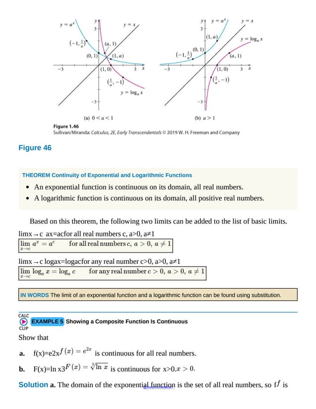
367. 47. limx→0 x2sin 1x
48. limx→0x1−cos 1x
49. limx→0 x21−cos 1x
50. limx→0x3+3x2 sin1x
In Problems 51–54, show that each statement is true.
51. limx→0 sin(ax)sin(bx)=ab ; b≠0
52. limx→0cos(ax)cos(bx)=1
53. limx→0 sin(ax)bx=ab ; b≠0
54. limx→0 1−cos(ax)bx=0 ; a≠0, b≠0
55. Show that limx→0 1−cos xx2=12.
56. Squeeze Theorem If 0≤ f (x)≤1 for every number x, show that
limx→0 [x2 f (x)]=0.
57. Squeeze Theorem If 0≤ f (x)≤M for every x, show that
limx→0 [x2 f(x)]=0.
58. The function f (x)=sin(πx)x is not defined at 0. Decide how to
define f (0) so that f is continuous at 0.
59. Define f (0) and f (1) so that the function f (x)=sin(πx)x(1−x)
is continuous on the interval [0,1].
@Seismicisolation
@Seismicisolation

368. 60. Is f(x)=sin xx if x≠01 if x=0 continuous at 0 ?
61. Is f(x)=1−cos xx if x≠00 if x=0 continuous at 0 ?
62. Squeeze Theorem Show that limx→0 xnsin1x=0, where n is a
positive integer.
(Hint: Look first at Problem 56.)
63. Prove limθ→0 sin θ=0.
(Hint: Use a unit circle as shown in the figure, first assuming 0<θ<π2. Then
use the fact that sin θ is less than the length of the arc AP, and the Squeeze
Theorem, to show that limθ→0+ sin θ=0. Then use a similar argument
with −π2<θ<0 to show limθ→0− sin θ=0. )
64. Prove limθ→0 cos θ=1. Use either the proof outlined in Problem 63 or a
proof using the result limθ→0 sin θ=0 and a Pythagorean identity.
@Seismicisolation
@Seismicisolation

369. 65. Without using limits, explain how you can decide where f(x)=cos(5x3+2x2−8x+1)
is continuous.
66. Explain the Squeeze Theorem. Draw a graph to illustrate your explanation.
Challenge Problems
67. Use the Sum Formulas sin(a+b)=sin a cos b+cos a sin b
and cos(a+b)=cos a cos b −sin a sin b
to show that the sine function and cosine
function are continuous on their domains.
68. Find limx→0 sin x2x.
69. Squeeze Theorem If f(x)=1 if x is rational0 if x is irrational
show that limx→0 [x f (x)]=0.
70. Suppose points A and B with coordinates (0,0) and (1,0), respectively,
are given. Let n be a number greater than 0, and let θ be an angle with the property
0<θ<π1+n. Construct a triangle ABC where AC¯ and AB¯
form the angle θ, and BC¯ and BA¯ form the angle n θ (see the figure
below). Let D be the point of intersection of AB¯ with the perpendicular from C
to AB¯. What is the limiting position of D as θ approaches 0 ?
1. = NOW WORK problem
= Graphing technology recommended
= Computer Algebra System recommended
@Seismicisolation
@Seismicisolation

370. * The Squeeze Theorem is also known as the Sandwich Theorem and the Pinching Theorem.
@Seismicisolation
@Seismicisolation

371. 1.5 Infinite Limits; Limits at Infinity; Asymptotes
OBJECTIVE When you finish this section, you should be able to:
1 Find infinite limits
2 Find the vertical asymptotes of a graph
3 Find limits at infinity
4 Find the horizontal asymptotes of a graph
5 Find the asymptotes of the graph of a rational function
We have described limx→c f (x)=L by saying if a function f is defined
everywhere in an open interval containing c, except possibly at c, then the value f (x)
can be made as close as we please to L by choosing numbers x sufficiently close to
c. Here c and L are real numbers. In this section, we extend the language of limits to
allow c to be ∞ or −∞ (limits at infinity) and to allow L to be ∞ or −∞
(infinite limits). These limits are useful for locating asymptotes that aid in graphing some
functions.
We begin with infinite limits.
RECALL The symbols ∞ (infinity) and −∞ (negative infinity) are not numbers. The symbol ∞
expresses unboundedness in the positive direction, and −∞ expresses unboundedness in the negative
direction.
1 Find Infinite Limits
Consider the function f (x)=1x2. Table 11 lists values of f for selected numbers
x that are close to 0 and Figure 48 shows the graph of f.
TABLE 11
x −0.01 −0.001 −0.0001 →0← 0.0001 0.001 0.01
f(x)=1x2
10,000 106 108
f (x)
becomes
unbounded
108 106 10,000
@Seismicisolation
@Seismicisolation

372. Figure 48 f(x)=1x2
As x approaches 0, the value of 1x2 increases without bound. Since the value of
1x2 is not approaching a single real number, the limit of f(x) as x approaches 0
does not exist. However, since the numbers are increasing without bound, we describe the
behavior of the function near zero by writing
limx→0 1x2=∞
and say that f (x)=1x2 has an infinite limit as x approaches 0.
In other words, a function f has an infinite limit at c if f is defined everywhere in an
open interval containing c, except possibly at c, and f (x) becomes unbounded when
x is sufficiently close to c.*
EXAMPLE 1 Investigating limx→0− 1x and limx→0+ 1x
Consider the function f (x)=1x. Table 12 shows values of f for selected numbers
x that are close to 0 and Figure 49 shows the graph of f.
TABLE 12
@Seismicisolation
@Seismicisolation

373. x −0.01 −0.001 −0.0001
→ 0
←
0.0001 0.001
f (x)=1x
−100 −1000 −10,000
f (x)
becomes
unbounded
10,000 1000
Figure 49 f (x)=1x
Here as x gets closer to 0 from the right, the value of f (x)=1x can be made
as large as we please. That is, 1x becomes unbounded in the positive direction. So,
limx→0+ 1x=∞
Similarly, the notation
limx→0− 1x=−∞
is used to indicate that 1x becomes unbounded in the negative direction as x approaches
0 from the left. ▪
So, there are four possible one-sided infinite limits of a function f at c :
@Seismicisolation
@Seismicisolation

374. limx→c− f (x)=∞,limx→c− f (x)=−∞,limx→c+ f (x)=∞,limx→c+ f (x)=−∞
See Figure 50 for illustrations of these possibilities.
Figure 50
In
the
first
figure,
the
left
hand
limit
of
the
function
as
x
approaches
c
is
infinity.
In
the
second
figure,
the
left
hand
limit
When we know the graph of a function, we can use it to investigate infinite limits.
EXAMPLE 2 Investigating an Infinite Limit
Investigate limx→0+ ln x.
Solution The domain of f(x)=ln x is {x|x>0}. Notice that the graph
of f(x)=ln x in Figure 51 decreases without bound as x approaches 0 from the
right. The graph suggests that
limx→0+ ln x=−∞
▪
@Seismicisolation
@Seismicisolation

375. Figure 51 f (x)=ln x
NOW WORK Problem 11.
Based on the graphs of the trigonometric functions in Figure 52, we have the following
infinite limits:
limx→π⁄2− tan x=∞ limx→π⁄2+tan x=−∞ limx→π⁄2− sec x=∞ limx→π⁄2+ sec x=
−∞limx→0− csc x=−∞ limx→0+ csc x=∞ limx→0− cot x=−∞ limx→0+ cot x=∞
Figure 52
Limits of quotients, in which the limit of the numerator is a nonzero number and the limit
of the denominator is 0, often result in infinite limits. (If the limits of both the numerator and
the denominator are 0, the quotient is called an indeterminate form. Limits of indeterminate
@Seismicisolation
@Seismicisolation

376. forms are discussed in Section 4.5.)
EXAMPLE 3 Finding an Infinite Limit
Find each limit:
a. limx→3+ 2x+1x−3
b. limx→1− x2ln x
Solution a. limx→3+ 2x+1x−3 is the right-hand limit of the quotient of two
functions, f (x)=2x+1 and g (x)=x−3. Since limx→3+ (x−3)=0,
we cannot use the Limit of a Quotient. So we need a different strategy. As
x approaches 3+, we have
limx→3+ (2x+1)=7andlimx→3+ (x−3)=0
Here the limit of the numerator is 7. The denominator is positive and approaching 0. So the
quotient is positive and becoming unbounded. We conclude that
limx→3+ 2x+1x−3=∞
b. As in (a), we cannot use the Limit of a Quotient because limx→1− ln x=0.
Here we have
limx→1− x2=1limx→1−ln x=0
We are seeking a left-hand limit, so for numbers close to 1 but less than 1, the denominator
ln x<0. So the quotient is negative and becoming unbounded. We conclude that
limx→1− x2ln x=−∞
▪
The discussion below may prove useful when finding limx→c− f (x)g (x),
@Seismicisolation
@Seismicisolation

377. where limx→c− f (x) is a nonzero number and limx→c− g (x)=0.
Analyzing limx→c− f (x)g (x) when limx→c− f (x)=L, L≠0,
and limx→c− g (x)=0.
If L>0 and g (x)<0 for numbers x close to c, but less than c, then
limx→c− f (x)g (x)=−∞
If L>0 and g (x)>0 for numbers x close to c, but less than c, then
limx→c− f (x)g (x)=∞
If L<0 and g (x)<0 for numbers x close to c, but less than c, then
limx→c− f (x)g (x)=∞
If L<0 and g (x)>0 for numbers x close to c, but less than c, then
limx→c− f (x)g (x)=−∞
Similar arguments are valid for right-hand limits.
NOW WORK Problem 27.
2 Find the Vertical Asymptotes of a Graph
Figure 53 illustrates the possibilities that can occur when a function has an infinite limit at c.
In each case, notice that the graph of f has a vertical asymptote x=c.
@Seismicisolation
@Seismicisolation

378. Figure 53
DEFINITION Vertical Asymptote
The line x=c is a vertical asymptote of the graph of the function f if any of the
following is true:
limx→c− f(x)=∞limx→c+ f(x)=∞limx→c− f(x)=−∞limx→c+ f(x)=−∞
For rational functions, a vertical asymptote may occur where the denominator equals 0.
EXAMPLE 4 Finding a Vertical Asymptote
Find any vertical asymptote(s) of the graph of f(x)=x(x−3)2.
Solution The domain of f is {x|x≠3}. Since 3 is the only number for which
the denominator of f equals zero, we construct Table 13 and investigate the one-sided limits
of f as x approaches 3. Table 13 suggests that
limx→3 x(x−3)2=∞
So, x=3 is a vertical asymptote of the graph of f.
TABLE 13
x 2.9 2.99 2.999 → 3 ← 3.001
f(x)=x(x−3)2
290 29,900 2,999,000
f(x)
becomes
unbounded
3,001,000
@Seismicisolation
@Seismicisolation

379. Figure 54 shows the graph of f (x)=x(x−3)2 and its vertical asymptote.
▪
Figure 54 f (x)=x(x−3)2
NOW WORK Problems 15 and 63 (find any vertical asymptotes).
3 Find Limits at Infinity
Now we investigate what happens as x becomes unbounded in either the positive direction
or the negative direction. Suppose as x becomes unbounded, the value of a function f
approaches some real number L. Then the number L is called the limit of f at infinity.
For example, the graph of f (x)=1x in Figure 55 suggests that as x becomes
unbounded in either the positive direction or the negative direction, the values f (x) get
closer to 0. Table 14 illustrates this for a few numbers x.
@Seismicisolation
@Seismicisolation

380. Figure 55 f (x)=1x
TABLE 14
x ±100 ±1000 ±10,000 ±100,000
x becomes
unbounded
f (x)=1x
±0.01 ±0.001 ±0.0001 ±0.00001 f (x)
approaches 0
Since f can be made as close as we please to 0 by choosing x sufficiently large, we
write
limx→∞ 1x=0
and say that the limit as x approaches infinity of f is equal to 0. Similarly, as x
becomes unbounded in the negative direction, the function f(x)=1x can be made as
close as we please to 0, and we write
limx→−∞ 1x=0
Although we do not prove limx→−∞ 1x=0 here, it can be proved using the
ε–δ Definition of a Limit at Infinity and is left as an exercise in Section 1.6.
The limit properties discussed in Section 1.2 hold for infinite limits. Although these
properties are stated below for limits as x→∞, they are also valid for limits as x→
@Seismicisolation
@Seismicisolation

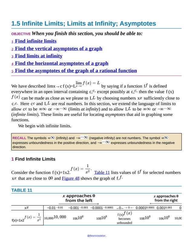
381. (1)
−∞.
THEOREM Properties of Limits at Infinity
If k is a real number, n≥2 is an integer, and the functions f and g approach real
numbers as x→∞, then the following properties are true:
limx→∞ A=A, where A is a constant
limx→∞ kf(x)=klimx→∞ f(x)
limx→∞ [f(x)±g(x)]=limx→∞ f(x)±limx→∞ g(x)
limx→∞ [f(x)g(x)]= limx→∞ f(x) limx→∞ g(x)
limx→∞ f(x)g(x)=limx→∞ f(x)limx→∞ g(x), provided
limx→∞ g(x)≠0
limx→∞ [f(x)]n=limx→∞ f(x)n
limx→∞ f(x)n=limx→∞ f(x)n, where f(x)>0 if n
is even
Since limx→∞ 1x=0 and limx→−∞ 1x=0, we can use
properties of limits at infinity to obtain two additional properties.
If p>0 is a rational number and k is any real number, then
limx→∞ kxp=0 andlimx→−∞ kxp=0
provided xp is defined when x<0.
You are asked to prove (1) in Problem 92.
@Seismicisolation
@Seismicisolation

382. EXAMPLE 5 Finding Limits at Infinity
Use property (1).
a. limx→∞ 5x3=0
b. limx→∞ 1x=0
c. limx→−∞ −6x1⁄3=0
d. limx→−∞ 45x8⁄3=0
▪
EXAMPLE 6 Finding Limits at Infinity
Find each limit.
a. limx→∞ 2+3x
b. limx→∞ 2+1x 13−2x3
c. limx→∞ 14 3x2+5x−1x2
Solution We use properties of limits at infinity and property (1).
a. limx→∞ 2+3x=limx→∞2+limx→∞ 3x=2+0=2
b. limx→∞ 2+1x
13−2x3=limx→∞2+1x⋅limx→∞13−2x3=limx→∞2+limx→∞ 1x⋅limx→∞ 13−limx→∞ 2
@Seismicisolation
@Seismicisolation

383. (2+0)13−0=23
c. limx→∞ 14 3x2+5x−1x2=14limx→∞ 3x2+5x−1x2=14limx→∞3+5x−1x2=14
limx→∞3+limx→∞ 5x−limx→∞ 1x2=14⋅3=34
▪
NOW WORK Problem 45.
For some algebraic functions involving a quotient, we find limits at infinity by dividing
the numerator and the denominator by the highest power of x that appears in the
denominator.
EXAMPLE 7 Finding a Limit at Infinity
Find each limit.
a. limx→∞ 3x3⁄2+5x1⁄2x3−x2⁄3
b. limx→∞ 4x2+10x−5
Solution a. Divide the numerator and the denominator by x3, the highest power of x
that appears in the denominator.
@Seismicisolation
@Seismicisolation

384. b. Divide the numerator and the denominator by x, the highest power of x that appears in
the denominator. But remember, since x2=|x|=x when x≥0, in the
numerator the divisor in the square root will be x2.
The graph of f(x)=4x2+10x−5 is shown in Figure 56.
Figure 56 f (x)=4x2+10x−5
@Seismicisolation
@Seismicisolation

385. (2)
(3)
(4)
NOW WORK Problems 47 and 57.
For polynomial and rational functions, there is an easier approach to finding limits at
infinity.
Limits at Infinity of Polynomial and Rational Functions
We begin by investigating limits at infinity of power functions. For any power function
p(x)=xn, if n is a positive integer, then p increases without bound as x→∞.
That is,
limx→∞ xn=∞n a positive integer
To investigate limx→−∞ xn, n a positive integer, we need to consider
whether n is even or odd. Remember, as x→−∞, is unbounded in the negative
direction, so x<0.
If n is positive and even, then xn>0 when x<0. If n is positive and odd,
then xn<0 when x<0. Since in both cases xn becomes unbounded as x→
−∞, we have
limx→−∞ xn=∞ if n is a positive even integerlimx→−∞xn=−∞ if n is a positive odd integer
Now consider a polynomial function, p(x)=anxn+an−1xn−1+⋯+a1 x+a0,an≠0.
To find limx→±∞ p(x),
factor out xn. Then
limx→±∞ p(x)=limx→±∞(anxn+an−1xn−1+⋯+a1x+a0)=limx→±∞xn an+an−1x+⋯+a1xn
−1+a0xn
Since limx→±∞ an+an−1x+⋯+a1xn−1+a0xn=an,
we have
@Seismicisolation
@Seismicisolation

386. limx→±∞ p(x)=anlimx→±∞xn
Using (2), (3), and (4), we can find the limit at infinity of any polynomial function.
EXAMPLE 8 Finding Limits at Infinity of a Polynomial Function
a. limx→∞ (3x3−x2+5x+1)=3limx→∞x3=∞Use (4) and (2).
b. limx→∞ (x5+2x)=limx→∞x5=∞Use (4) and (2).
c. limx→−∞ (2x4−x2+2x+8)=2limx→−∞x4=∞Use (4) and (3).
d. limx→−∞ (x3+10x+7)=limx→−∞x3=−∞Use (4) and (3).
▪
So, for a polynomial function, as x becomes unbounded in either the positive direction
or the negative direction, the polynomial function is also unbounded. In other words,
polynomial functions have an infinite limit at infinity.
Since a rational function R is the quotient of two polynomial functions p and q,
where q is not the zero polynomial, we can find a limit at infinity for a rational function
using only the leading terms of p and q.
Consider the rational function R(x)=anxn+an−1xn−1+⋯+a1 x+a0bmxm+bm−1xm−1+⋯
+b1 x+b0, where an≠0, bm≠0.
Then we simplify R as follows:
R(x)=xn an+an−1x+⋯+a1xn−1+a0xnxm bm+bm−1x+⋯+b1xm−1+b0xm
Since limx→∞ an+an−1x+⋯+a1xn−1+a0xn=an
@Seismicisolation
@Seismicisolation

387. (5)
and limx→∞ bm+bm−1x+⋯+b1xm−1+b0xm=bm,
we have
limx→∞ R(x)=limx→∞ xnxm⋅limx→∞an+an−1x+⋯+a1xn−1+a0xnlimx→∞bm+bm−1x+⋯
+b1xm−1+b0xm=anbmlimx→∞ xnxm
Or more generally,
limx→±∞ R(x)=limx→±∞ anxn+an−1xn−1+⋯+a1 x+a0bmxm+bm−1xm−1+⋯
+b1 x+b0=anbmlimx→±∞ xnxm
EXAMPLE 9 Finding Limits at Infinity of a Rational Function
Find each limit.
a. limx→∞ 3x2−2x+8x2+1
b. limx→∞ 4x2−5xx3+1
c. limx→∞ 5x4−3x22x2+1
Solution Each of these limits at infinity involve a rational function, so we use (5).
a. limx→∞ 3x2−2x+8x2+1=3limx→∞ x2x2=3
b. limx→∞ 4x2−5xx3+1=4limx→∞ x2x3=4limx→∞ 1x=0
c. limx→∞ 5x4−3x22x2+1=52limx→∞ x4x2=52limx→∞x2=∞
@Seismicisolation
@Seismicisolation

388. ▪
The graphs of the functions f(x)=3x2−2x+8x2+1 and
G(x)=4x2−5xx3+1 are shown in Figure 57(a) and (b), respectively. Notice
how each graph behaves as x becomes unbounded in the positive direction. The graph of
the function H(x)=5x4−3x22x2+1, which has an infinite limit at infinity,
is shown in Figure 57(c).
Figure 57
NOW WORK Problems 49 and 59.
Other Infinite Limits at Infinity
We have seen that all polynomial functions have infinite limits at infinity, and some rational
functions have infinite limits at infinity. Other functions also have an infinite limit at infinity.
For example, consider the function f(x)=ex.
The graph of the exponential function, shown in Figure 58, suggests that
limx→−∞ ex=0limx→∞ex=∞
@Seismicisolation
@Seismicisolation

389. Figure 58 f(x)=ex
These limits are supported by the information in Table 15.
TABLE 15
x −1 −5 −10 −20
x
approaches
−∞
f(x)=ex 0.36788 0.00674 0.00005 2×10−9
f(x)
approaches
0
x 1 5 10 20
x
approaches
∞
f(x)=ex e≈2.71828 148.41 22,026 4.85×108
f(x)
becomes
unbounded
EXAMPLE 10 Finding the Limit at Infinity of g(x)=ln x
Find limx→∞ ln x.
Solution Table 16 and the graph of g(x)=ln x in Figure 59 suggest that
g(x)=ln x has an infinite limit at infinity. That is,
limx→∞ ln x=∞
TABLE 16
@Seismicisolation
@Seismicisolation

390. x e10 e100 e1000 e10,000 e100,000 →x becomes
unbounded
g(x)=ln x 10 100 1000 10,000 100,000
→g(x)
becomes
unbounded
▪
Figure 59 g(x)=ln x
Now let’s compare the graph of f(x)=ex in Figure 58, the graph of g(x)=lnx
in Figure 59, and the graph of h(x)=x2 in Figure 60. As x becomes
unbounded in the positive direction, all three of the functions increase without bound. But in
Table 17, f(x)=ex approaches infinity more rapidly than h(x)=x2,
which approaches infinity more rapidly than g(x)=lnx.
@Seismicisolation
@Seismicisolation

391. Figure 60 h(x)=x2
TABLE 17
x 10 50 100 1000
f(x)=ex 22,026 5.185×1021 2.688×1043 e1000
h(x)=x2 100 2500=2.5×103 1.0×104 1.0×106
g(x)=ln x 2.303 3.912 4.605 6.908
EXAMPLE 11 Application: Decomposition of Salt in Water
Salt (NaCl) dissolves in water into sodium (Na+) ions and chloride (Cl−) ions
according to the law of uninhibited decay
A(t)=A0ekt
where A=A(t) is the amount (in kilograms) of undissolved salt present at time t
(in hours), A0 is the original amount of undissolved salt, and k is a negative number that
represents the rate of dissolution.
a. If initially there are 25 kilograms (kg) of undissolved salt and after 10 hours (h) there are
15 kg of undissolved salt remaining, how much undissolved salt is left after one day?
b. How long will it take until 12kg of undissolved salt remains?
c. Find limt→∞ A(t).
d. Interpret the answer found in (c).
@Seismicisolation
@Seismicisolation

392. NEED TO REVIEW? Solving exponential equations is discussed in Section P.5, pp. 48–49.
Solution a. Initially, there are 25 kg of undissolved salt, so A(0)=A0=25.
To find the number k in A(t)=A0ekt, we use the fact that at t=10, then
A(10)=15. That is,
A(10)=15=25e10kA(t)=A0ekt,A0=25;A(10)=15;t=10e10k=3510k=ln 35k=110 ln0.6
So, A(t)=25e110 ln0.6t. The amount of undissolved salt that
remains after one day (24 h ) is
A(24)=25e110 ln0.624≈7.337 kg
b. We want to find t so that A(t)=25e110 ln0.6t=12 kg. Then
12=25e110 ln0.6te110 ln0.6t=150110 ln0.6t=ln 150t≈76.582
After approximately 76.6 h, 12 kg of undissolved salt will remain.
c. Since 110 ln0.6≈−0.051, we have limt→∞ A(t)=limt→∞(25e
−0.051t)=limt→∞ 25e0.051t=0
d. As t becomes unbounded, the amount of undissolved salt approaches 0 kg.
Eventually, there will be no undissolved salt in the water. ▪
@Seismicisolation
@Seismicisolation

393. NOW WORK Problem 79.
4 Find the Horizontal Asymptotes of a Graph
Limits at infinity have an important geometric interpretation. When limx→∞ f(x)=M,
it means that as x becomes unbounded in the positive direction, the value
of f can be made as close as we please to a number M. That is, the graph of y=f(x)
is as close as we please to the horizontal line y=M by choosing x
sufficiently large. Similarly, limx→−∞ f(x)=L means that the graph of
y=f(x) is as close as we please to the horizontal line y=L for x unbounded
in the negative direction. These lines are horizontal asymptotes of the graph of f.
DEFINITION Horizontal Asymptote
The line y=L is a horizontal asymptote of the graph of a function f for x
unbounded in the negative direction if limx→−∞ f (x)=L.
The line y=M is a horizontal asymptote of the graph of a function f for x
unbounded in the positive direction if limx→∞ f (x)=M.
In Figure 61, y=L is a horizontal asymptote as x→−∞ because limx→
−∞ f(x)=L. The line y=M is a horizontal asymptote as x→∞
because limx→∞ f(x)=M. To identify horizontal asymptotes, we find the
limits of f at infinity.
@Seismicisolation
@Seismicisolation

394. Figure 61
EXAMPLE 12 Finding the Horizontal Asymptotes of a Graph
Find the horizontal asymptotes, if any, of the graph of f(x)=3x−24x−1.
Solution We examine the two limits at infinity:limx→−∞ 3x−24x−1 and
limx→∞ 3x−24x−1.
Since limx→−∞ 3x−24x−1=34, the line y=34 is a horizontal
asymptote of the graph of f for x unbounded in the negative direction.
Since limx→∞ 3x−24x−1=34, the line y=34 is a horizontal
asymptote of the graph of f for x unbounded in the positive direction. ▪
Figure 62 shows the graph of f(x)=3x−24x−1 and the horizontal
asymptote y=34.
@Seismicisolation
@Seismicisolation

395. Figure 62 f(x)=3x−24x−1
NOW WORK Problem 63 (find any horizontal asymptotes).
5 Find the Asymptotes of the Graph of a Rational Function
In the next example we find the horizontal asymptotes and vertical asymptotes, if any, of the
graph of a rational function.
EXAMPLE 13 Finding the Asymptotes of the Graph of a Rational Function
Find any asymptotes of the graph of the rational function R(x)=3x2−122x2−9x+10.
Solution We begin by factoring R.
R(x)=3x2−122x2−9x+10=3(x−2)(x+2)(2x−5)(x−2)
The domain of R is x|x≠52 and x≠2. Since R is a rational
function, it is continuous on its domain, that is, all real numbers except x=52 and x=2.
@Seismicisolation
@Seismicisolation

396. To check for vertical asymptotes, we find the limits as x approaches 52 and 2.
First we consider limx→52− R(x).
limx→52− R(x)=limx→52− 3(x−2)(x+2)(2x−5)(x−2)=limx→52− 3(x+2)2x
−5=3limx→52− x+22x−5=−∞
That is, as x approaches 52 from the left, R becomes unbounded in the negative
direction. The graph of R has a vertical asymptote on the left at x=52.
To determine the behavior to the right of x=52, we find the right-hand limit.
limx→52+ R(x)=limx→52+ 3(x+2)2x−5=3limx→52+ x+22x−5=∞
As x approaches 52 from the right, R becomes unbounded in the positive direction.
The graph of R has a vertical asymptote on the right at x=52.
Next we consider limx→2 R(x).
limx→2 R(x)=limx→2 3(x−2)(x+2)(2x−5)(x−2)=limx→2 3(x+2)2x−5=3(2+2)2⋅2−5=12−1=
−12
Since the limit is not infinite, the function R does not have a vertical asymptote at 2.
Since 2 is not in the domain of R, the graph of R has a hole at the point (2,−12).
To check for horizontal asymptotes, we find the limits at infinity.
The line y=32 is a horizontal asymptote of the graph of R for x unbounded in the
@Seismicisolation
@Seismicisolation

397. negative direction and for x unbounded in the positive direction. ▪
The graph of R and its asymptotes are shown in Figure 63. Notice the hole in the graph
at the point (2,−12).
Figure 63 R(x)=3x2−122x2−9x+10
As
x
approaches
5
by
2
from
the
right,
R
tends
to
infinity,
as
x
1.5 Assess Your Understanding
Concepts and Vocabulary
1. True or False ∞ is a number.
2.
a. limx→0− 1x=_____
b. limx→0+ 1x=_____
c. limx→0+ ln x=_____
3. True or False The graph of a rational function has a vertical asymptote at every number
x at which the function is not defined.
@Seismicisolation
@Seismicisolation

398. 4. If limx→4f(x)=∞, then the line x=4 is a(n) _____ asymptote of the
graph of f.
5.
a. limx→∞ 1x=_____
b. limx→∞ 1x2=_____
c. limx→∞ ln x=_____
6. True or False limx→−∞ 5=0.
7.
a. limx→−∞ ex=_____
b. limx→∞ ex=_____
c. limx→∞ e−x=_____
8. True or False The graph of a function can have at most two horizontal asymptotes.
Skill Building
In Problems 9–16, use the accompanying graph of y=f(x).
9. Find limx→∞ f(x).
10. Find limx→−∞ f(x).
11. Find limx→−1− f(x).
12. Find limx→−1+ f(x).
13. Find limx→3− f(x).
14. Find limx→3+ f(x).
15. Identify all vertical asymptotes.
16. Identify all horizontal asymptotes.
@Seismicisolation
@Seismicisolation

399. As
x
approaches
negative
infinity,
limit
of
f
tends
to
0.
As
x
approaches
minus
1
from
the
left
or
right,
limit
of
f
In Problems 17–26, use the graph below of y=f(x).
17. Find limx→∞ f(x).
18. Find limx→−∞ f(x).
19. Find limx→−3− f(x).
20. Find limx→−3+ f(x).
21. Find limx→0− f(x).
22. Find limx→0+ f(x).
23. Find limx→4− f(x).
24. Find limx→4+ f(x).
25. Identify all vertical asymptotes.
26. Identify all horizontal asymptotes.
@Seismicisolation
@Seismicisolation

400. f
is
not
defined
at
(0,
0).
As
x
approaches
negative
infinity,
limit
of
f
tends
to
0.
As
x
approaches
minus
3
In Problems 27–42, find each limit.
27. limx→2− 3xx−2
28. limx→−4+ 2x+1x+4
29. limx→2+ 5x2−4
30. limx→1− 2xx3−1
31. limx→−1+ 5x+3x(x+1)
32. limx→0− 5x+35x(x−1)
33. limx→−3− 1x2−9
34. limx→2+ xx2−4
@Seismicisolation
@Seismicisolation

401. 35. limx→3 1−x(3−x)2
36. limx→−1 x+2(x+1)2
37. limx→π− cot x
38. limx→−π⁄2− tan x
39. limx→π⁄2+ csc(2x)
40. limx→−π⁄2− sec x
41. limx→−1+ ln(x+1)
42. limx→1+ ln(x−1)
In Problems 43–60, find each limit.
43. limx→∞ 5x2+4
44. limx→−∞ 1x2−9
45. limx→∞ 2x+45x
46. limx→∞ x+1x
47. limx→∞ x3⁄2+2x−x1⁄25x−x1⁄2
48. limx→∞ 6x2+x3⁄42x2+x3⁄2−2x1⁄2
49. limx→−∞ x2+1x3−1
50. limx→∞ x2−2x+1x3+5x+4
@Seismicisolation
@Seismicisolation

402. 51. limx→∞ 3x2x+5−x2+14x2+8
52. limx→∞ 1x2+x+4−x+13x−1
53. limx→−∞ 2ex5x+13x
54. limx→−∞ exx2+x−32x3−x2
55. limx→∞ x+23x−4
56. limx→∞ 3x3+2x2+6
57. limx→∞ 3x2−1x2+4
58. limx→∞ 16x3+2x+12x3+3x2⁄3
59. limx→−∞ 5x3x2+1
60. limx→−∞ x4x−2
In Problems 61–66, find any horizontal or vertical asymptotes of the graph of f.
61. f (x)=3+1x
62. f (x)=2−1x2
63. f (x)=x2x2−1
64. f (x)=2x2−1x2−1
@Seismicisolation
@Seismicisolation

403. 65. f (x)=2x2−x+102x−3
66. f (x)=x2+5x3x−6
In Problems 67–72, for each rational function R:
a. Find the domain of R.
b. Find any horizontal asymptotes of R.
c. Find any vertical asymptotes of R.
d. Discuss the behavior of the graph at numbers where R is not defined.
67. R (x)=−2x2+12x3+4x2
68. R (x)=x3x4−1
69. R (x)=x2+3x−102x2−7x+6
70. R (x)=x(x−1)2(x+3)3
71. R (x)=x3−1x−x2
72. R (x)=4x5x3−1
Applications and Extensions
In Problems 73 and 74:
a. Sketch a graph of a function f that has the given properties.
b. Define a function that describes the graph.
73. f(3)=0 limx→∞ f(x)=1 limx→−∞ f(x)=1
limx→1− f(x)=∞ limx→1+ f(x)=−∞
74. f(2)=0 limx→∞ f(x)=0 limx→−∞ f(x)=0 limx→0 f(x)=∞
limx→5− f(x)=
@Seismicisolation
@Seismicisolation

404. −∞ limx→5+ f(x)=∞
75. Newton’s Law of Cooling Suppose an object is heated to a temperature u0. Then at
time t=0, the object is put into a medium with a constant lower temperature T
causing the object to cool. Newton’s Law of Cooling states that the temperature u of
the object at time t is given by u=u(t)=(u0−T)ekt+T,
where k<0 is a constant.
a. Find limt→∞ u(t). Is this the value you expected? Explain why or why
not.
b. Find limt→0+ u(t). Is this the value you expected? Explain why or why
not.
Source: Submitted by the students of Millikin University.
76. Environment A utility company burns coal to generate electricity. The cost C, in
dollars, of removing p% of the pollutants emitted into the air is
C=70,000p100−p0≤p<100
Find the cost of removing:
a. 45% of the pollutants.
b. 90% of the pollutants.
c. Find limp→100− C.
d. Interpret the answer found in (c).
77. Pollution Control The cost C, in thousands of dollars, to remove a pollutant from a
lake is
C(x)=5x100−x0≤x<100
where x is the percent of pollutant removed. Find limx→100− C(x).
Interpret your answer.
78. Population Model A rare species of insect was discovered in the Amazon Rain Forest.
To protect the species, entomologists declared the insect endangered and transferred 25
insects to a protected area. The population P of the new colony t days after the
transfer is
@Seismicisolation
@Seismicisolation

405. P(t)=50(1+0.5t)2+0.01t
a. What is the projected size of the colony after 1 year (365 days)?
b. What is the largest population that the protected area can sustain? That is, find limt→∞ P(t).
c. Graph the population P as a function of time t.
d. Use the graph from (c) to describe the regeneration of the insect population. Does the graph support the answer to
(b)?
79. Population of an Endangered Species Often environmentalists capture several
members of an endangered species and transport them to a controlled environment
where they can produce offspring and regenerate their population. Suppose six
American bald eagles are captured, tagged, transported to Montana, and set free. Based
on past experience, the environmentalists expect the population to grow according to the
model
P(t)=5001+82.3e−0.162t
where t is measured in years.
a. If the model is correct, how many bald eagles can the environment sustain? That is, find limt→∞ P(t).
b. Graph the population P as a function of time t.
c. Use the graph from (b) to describe the growth of the bald eagle population. Does the graph support the answer to
(a)?
80. Hailstones Hailstones typically originate at an altitude of about 3000 meters (m).
If a hailstone falls from 3000 m with no air resistance, its
speed when it hits the ground would be about 240 meters⁄second (m⁄s),
which is 540 miles⁄hour (mi⁄h)! That
would be deadly! But air resistance slows the hailstone considerably. Using a simple
model of air resistance, the speed v=v(t) of a hailstone of mass m as a
function of time t is given by v(t)=mgk (1−e−kt⁄m) m⁄s,
where g=9.8 m⁄s2 and k is a constant that depends on the size of the
hailstone, its mass, and the conditions of the air. For a hailstone with a diameter
d=1 centimeter (cm) and mass m=4.8×10−4 kg, k
has been measured to be 3.4×10−4 kg⁄s.
@Seismicisolation
@Seismicisolation

406. a. Determine the limiting speed of the hailstone by finding limt→∞ v(t). Express your answer in meters
per second and miles per hour, using the fact that 1 mi⁄h≈0.447 m⁄s. This speed is
called the terminal speed of the hailstone.
b. Graph v=v(t). Does the graph support the answer to (a)?
81. Damped Harmonic Motion The motion of a spring is given by the function
x(t)=1.2e−t⁄2cos t+2.4e−t⁄2sint
where x is the distance in meters from the the equilibrium position and t is the
time in seconds.
a. Graph y=x(t). What is limt→∞ x(t), as suggested by the graph?
b. Find limt→∞ x(t).
c. Compare the results of (a) and (b). Is the answer to (b) supported by the graph in (a)?
82. Decomposition of Chlorine in a Pool Under certain water conditions, the free chlorine
(hypochlorous acid, HOCl) in a swimming pool decomposes according to the
law of uninhibited decay, C=C(t)=C(0)ekt, where C=C(t)
is the amount (in parts per million, ppm) of free chlorine present at time t (in
hours) and k is a negative number that represents the rate of decomposition. After
shocking his pool, Ben immediately tested the water and found the concentration of free
chlorine to be C0=C(0)=2.5 ppm. Twenty-four hours later, Ben
tested the water again and found the amount of free chlorine to be 2.2 ppm.
a. What amount of free chlorine will be left after 72 hours?
b. When the free chlorine reaches 1.0 ppm, the pool should be shocked again. How long can Ben go
before he must shock the pool again?
c. Find limt→∞ C(t).
d. Interpret the answer found in (c).
83. Decomposition of Sucrose Reacting with water in an acidic solution at 35 ∘C,
the amount A of sucrose (C12H22O11) decomposes into glucose
(C6H12O6) and fructose (C6H12O6) according to the law of
uninhibited decay A=A(t)=A(0)ekt, where A=A(t) is the
amount (in moles) of sucrose present at time t (in minutes) and k is a negative
number that represents the rate of decomposition. An initial amount
A0=A(0)=0.40 mole of sucrose decomposes to 0.36 mole
@Seismicisolation
@Seismicisolation

407. in 30 minutes.
a. How much sucrose will remain after 2 hours?
b. How long will it take until 0.10 mole of sucrose remains?
c. Find limt→∞ A(t).
d. Interpret the answer found in (c).
84. Macrophotography A camera lens can be approximated by a thin lens. A thin lens of
focal length f obeys the thin-lens equation 1f=1p+1q, where p>f is
the distance from the lens to the object being photographed and q is the distance from
the lens to the image formed by the lens. See the figure below. To photograph an object,
the objects’s image must be formed on the photo sensors of the camera, which can only
occur if q is positive.
a. Is the distance q of the image from the lens continuous as the distance of the object being photographed
approaches the focal length f of the lens? (Hint: First solve the thin-lens equation for q and then find
limp→f+ q. )
b. Use the result from (a) to explain why a camera (or any lens) cannot focus on an object placed close to its focal
length.
In Problems 85 and 86, find conditions on a,b,c, and d so that the graph of f has no
horizontal or vertical asymptotes.
85. f(x)=ax3+bcx4+d
86. f(x)=ax+bcx+d
87. Explain why the following properties are true. Give an example of each.
@Seismicisolation
@Seismicisolation

408. a. If n is an even positive integer, then limx→c 1(x−c)n=∞.
b. If n is an odd positive integer, then limx→c− 1(x−c)n=−∞.
c. If n is an odd positive integer, then limx→c+ 1(x−c)n=∞.
88. Explain why a rational function, whose numerator and denominator have no common
zeros, will have vertical asymptotes at each point of discontinuity.
89. Explain why a polynomial function of degree 1 or higher cannot have any asymptotes.
90. If P and Q are polynomials of degree m and n, respectively, discuss
limx→∞ P(x)Q(x) when:
a. m>n
b. m=n
c. m<n
91. a. Use a table to investigate limx→∞ 1+1xx.
b. Find limx→∞ 1+1xx.
c. Compare the results from (a) and (b). Explain the possible causes of any discrepancy.
92. Prove that limx→±∞ kxp=0, for any real number k, and p>0,
provided xp is defined when x<0.
Challenge Problems
93. Kinetic Energy At low speeds the kinetic energy K, that is, the energy due to the
motion of an object of mass m and speed v, is given by the formula
K=K(v)=12 mv2. But this formula is only an approximation to the
general formula, and works only for speeds much less than the speed of light, c. The
general formula, which holds for all speeds, is
@Seismicisolation
@Seismicisolation

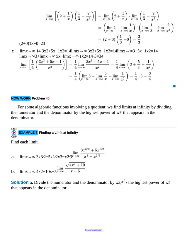
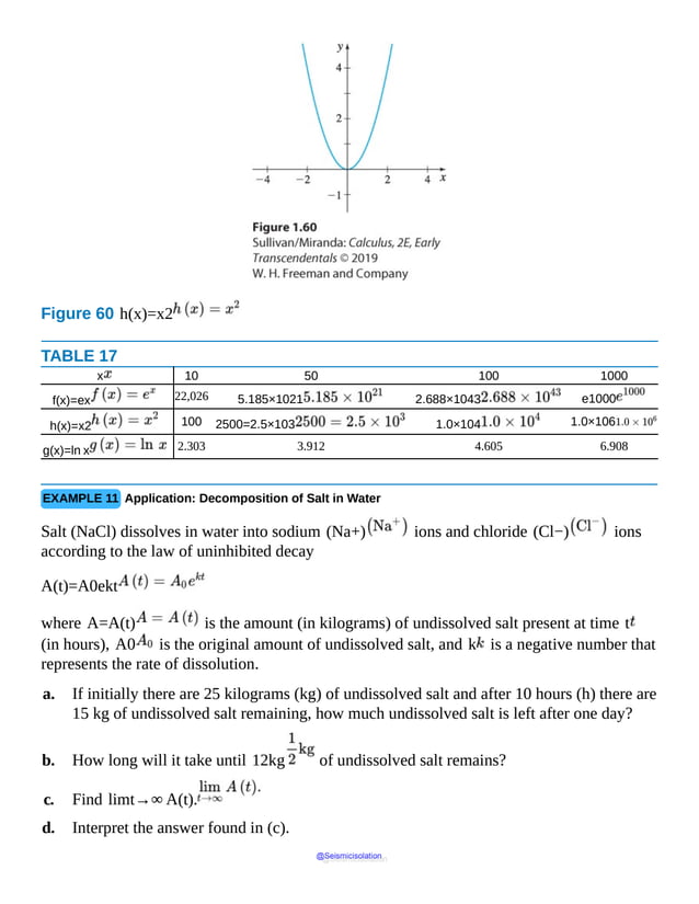
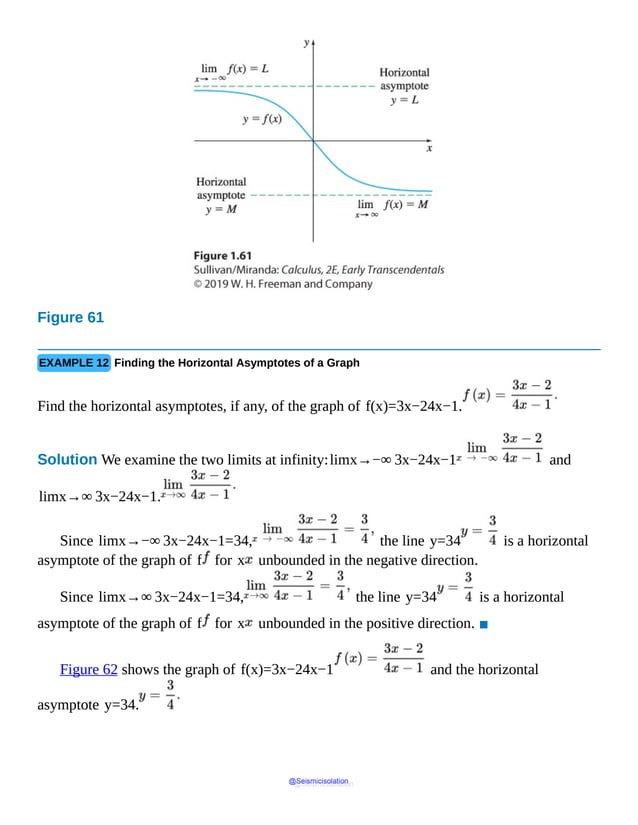
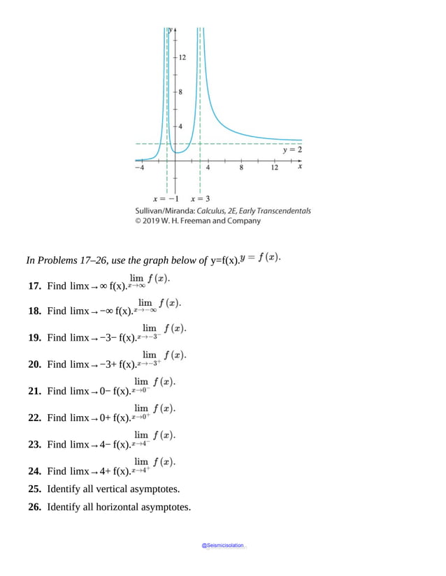
409. Kgen(v)=mc2[11−v2c2−1]
a. As an object is accelerated closer and closer to the speed of light, what does its kinetic energy Kgen
approach?
b. What does the result suggest about the possibility of reaching the speed of light?
94. limx→∞ 1+1x=1, but limx→∞1+1xx>1.
Discuss why the property limx→∞[f(x)]n=limx→∞ f(x)n
cannot be used to find the second limit.
1. = NOW WORK problem
= Graphing technology recommended
= Computer Algebra System recommended
* A precise definition of an infinite limit is given in Section 1.6.
@Seismicisolation
@Seismicisolation

410. 1.6 The ε−δ Definition of a Limit
OBJECTIVE When you finish this section, you should be able to:
1 Use the ε -δ definition of a limit
Throughout the chapter, we stated that we could be sure a limit was correct only if it was
based on the ε -δ definition of a limit. In this section, we examine this definition and how
to use it to prove a limit exists, to verify the value of a limit, and to show that a limit does not
exist.
Consider the function f defined by
f(x)=3x+1 if x≠210 if x=2
whose graph is given in Figure 64.
Figure 64 f(x)=3x+1 if x≠210 if x=2
As x gets closer to 2, but x≠2, the value f(x) gets closer to 7. If in fact,
@Seismicisolation
@Seismicisolation

411. by taking x close enough to 2, we can make f(x) as close to 7 as we please, then
limx→2 f(x)=7.
For example, if we want f(x) to differ from 7 by less than 0.3, then |f(x)−7|
<0.3, and
−0.3<f(x)−7<0.3−0.3<(3x+1)−7<0.3−0.3<3x−6<0.3−0.3<3(x−2)<0.3−0.33<x
−2<0.33−0.1<x−2<0.1|x−2|<0.1
That is, whenever x≠2 and x differs from 2 by less than 0.1, then f(x)
differs from 7 by less than 0.3.
Now generalizing the question, we ask, for x≠2, how close must x be to 2 to
guarantee that f(x) differs from 7 by less than any given positive number ε? (ε
might be extremely small.) The statement “f(x) differs from 7 by less than ε ” means
|f(x)−7|<ε−ε<f(x)−7<ε7−ε<f(x)<7+εAdd 7 to each
expression.7−ε<3x+1<7+εSince x≠2, then f(x)=3x+1.
Now we want the middle term to be x−2. This is done as follows:
7−ε<3x+1<7+ε6−ε<3x<6+εSubtract 1 from each expression.2−ε3<x<2+ε3Divide each
expression by 3.−ε3<x−2<ε3 Subtract 2 from each expression.|x−2|<ε3
The answer to our question is
@Seismicisolation
@Seismicisolation

412. “x must be within ε3 of 2, but not equal to 2, to guarantee that f(x) is within
ε of 7. ”
That is, whenever x≠2 and x differs from 2 by less than ε3, then f(x)
differs from 7 by less than ε, which can be restated as
whenever [x≠2 and x differs from 2by less than δ=ε3] then [f(x) differs from 7by less than ε]
We shorten the phrase “ε is any given positive number” by writing ε>0. Then the
statement on the right is written
f(x)−7<ε
Similarly, the statement “x differs from 2 by less than δ ” is written |x−2|<δ.
The statement “x≠2 ” is handled by writing
0<|x−2|<δ
So for our example, we write:
Given any ε>0, then there is a number δ>0 so that
whenever 0<|x−2|<δ,then |f(x)−7|<ε
Since the number δ=ε3 satisfies the inequalities for any number ε>0, we
conclude that limx→2 f(x)=7.
NOW WORK Problem 41.
This discussion above explains the definition of the limit of a function.
DEFINITION Limit of a Function
Let f be a function defined everywhere in an open interval containing c, except possibly
at c. Then the limit as x approaches c of f(x) is L, written
limx→c f(x)=L
if, given any number ε>0, there is a number δ>0 so that
@Seismicisolation
@Seismicisolation

413. whenever0<|x−c|<δthen|f(x)−L|<ε
This definition is commonly called the ε−δ definition of a limit of a function.
Figure 65 illustrates the definition for three choices of ε. Compare Figures 65(a) and
65(b). Notice that in Figure 65(b), the smaller ε requires a smaller δ. Figure 65(c)
illustrates what happens if δ is too large for the choice of ε ; here there are values of f,
for example, at x1 and x2, for which |f(x)−L|≮ε.
Figure 65
Diagram
shows
curve
depicting
the
function
f
containing
point
(c,
L).
The
rectangular
region
centered
about
the
point
(c,
L)
has
1 Use the ε−δ Definition of a Limit
EXAMPLE 1 Using the ε−δ Definition of a Limit
Use the ε–δ definition of a limit to prove limx→–1 (1−2x)=3.
Solution Given any ε>0, we must show there is a number δ>0 so that
whenever0 <|x−(−1)|=|x+1|<δ then|(1−2x)−3|<ε
The idea is to find a connection between |x−(−1)|=|x+1| and |(1−2x)−3|.
Since
|(1−2x)−3|=|−2x−2|=|−2(x+1)|=|−2|⋅|x+1|=2|x+1|
we see that for any ε>0,
whenever |x−(−1)|=|x+1|<δ=ε2 then|(1−2x)−3|=2|x+1|<2δ=ε
That is, given any ε>0 there is a δ, δ=ε2, so that whenever 0<|x−(−1)|<δ,
@Seismicisolation
@Seismicisolation

414. we have |(1−2x)−3|<ε. This proves that
limx→–1 (1−2x)=3. ▪
NOW WORK Problem 21.
A geometric interpretation of the ε–δ definition is shown in Figure 66. We see that
whenever x on the horizontal axis is between −1−δ and −1+δ, but not equal
to −1, then f(x) on the vertical axis is between the horizontal lines y=3+ε
and y=3−ε. So, limx→–1 f(x)=3 describes the behavior of f near
−1.
Figure 66 limx→–1 (1−2x)=3
EXAMPLE 2 Using the ε−δ Definition of a Limit
Use the ε–δ definition of a limit to prove that
a. limx→c A=A, where A and c are real numbers
b. limx→c x=c, where c is a real number
Solution a. f(x)=A is the constant function whose graph is a horizontal line.
@Seismicisolation
@Seismicisolation

415. Given any ε>0, we must find δ>0 so that whenever 0<|x−c|<δ,
then f(x)−A<ε.
Since A−A=0, then f(x)−A<ε no matter what positive
number δ is used. That is, any choice of δ guarantees that whenever 0<|x−c|<δ,
then f(x)−A<ε.
b. f(x)=x is the identity function. Given any ε>0, we must find δ so that
whenever 0<|x−c|<δ, then |f(x)−c|=|x−c|<ε. The
easiest choice is to make δ=ε. That is, whenever 0<|x−c|<δ=ε,
then
▪
Some observations about the ε–δ definition of a limit are given below:
The limit of a function in no way depends on the value of the function at c.
In general, the size of δ depends on the size of ε.
For any ε, if a suitable δ has been found, any smaller positive number will also
work for δ. That is, δ is not uniquely determined when ε is given.
EXAMPLE 3 Using the ε−δ Definition of a Limit
Prove: limx→2 x2=4
Solution Given any ε>0, we must show there is a number δ>0 so that
whenever 0 <|x−2|<δ then|x2−4|<ε
To establish a connection between x2−4 and x−2, we write x2−4 as
x2−4=(x+2)(x−2)=x+2⋅x−2
Now if we can find a number K for which x+2<K, then we can choose δ=εK.
To find K, we restrict x to some interval centered at 2. For example, suppose the
@Seismicisolation
@Seismicisolation

416. distance between x and 2 is less than 1. Then
|x−2|<1 −1<x−2<1 1<x<3Simplify.1+2<x+2<3+2Add 2 to each part.3<x+2<5
In particular, we have |x+2|<5. It follows that whenever |x−2|<1,
|x2−4|=|x+2|⋅|x−2|<5|x−2|
If |x−2|<δ=ε5, then x2−4<5|x−2|<5⋅ε5=ε, as
desired.
But before choosing δ=ε5, we must remember that there are two constraints on |x
−2|. Namely,
|x−2|<1and|x−2|<ε5
To ensure that both inequalities are satisfied, we select δ to be the smaller of the
numbers 1 and ε5, abbreviated as δ=min1,ε5. Now
whenever|x−2|<δ=min1,ε5then|x2−4|<ε
proving limx→2 x2=4. ▪
NOW WORK Problem 23.
In Example 3, the decision to restrict x so that |x−2|<1 was completely
arbitrary. However, since we are looking for x close to 2, the interval chosen should be
small. In Problem 40, you are asked to verify that if we had restricted x so that |x−2|<13,
then the choice for δ would be less than or equal to the smaller of 13 and
@Seismicisolation
@Seismicisolation

417. 3ε13 ; that is, δ≤min13,3ε13.
EXAMPLE 4 Using the ε−δ Definition of a Limit
Prove limx→c 1x=1c, where c>0.
Solution The domain of f(x)=1x is {x|x≠0}.
For any ε>0, we need to find a positive number δ so that whenever 0<|x−c|<δ,
then 1x−1c<ε. For x≠0, and c>0, we have
1x−1c=c−xxc=|c−x|| x|⋅|c |=|x−c|c|x |
The idea is to find a connection between
|x−c|and|x−c|c|x |
We proceed as in Example 3. Since we are interested in x near c, we restrict x to a small
interval around c, say, |x−c|<c2. Then
−c2<x−c<c2 c2<x<3c2Add c to each expression.
Since c>0, then x>c2>0, and 1x<2c. Now
1x−1c=|x−c|c|x |<2c2⋅|x−c|Substitute 1|x|<2c.
We can make 1x−1c<ε by choosing δ=c22 ε. Then
whenever|x−c|<δ=c22 ε,we have 1x−1c<2c2⋅|x−c|<2c2⋅c22⋅ε=ε
@Seismicisolation
@Seismicisolation

418. But remember, there are two restrictions on |x−c|.
|x−c|<c2and|x−c|<c22⋅ε
So, given any ε>0, we choose δ=minc2,c22⋅ε. Then
whenever 0<|x−c|<δ, we have 1x−1c<ε. This proves
limx→c 1x=1c, c>0. ▪
NOW WORK Problem 25.
The ε–δ definition of a limit can be used to show that a limit does not exist or that a
limit is not equal to a specific number. Example 5 illustrates how the ε–δ definition of a
limit is used to show that a limit is not equal to a specific number.
EXAMPLE 5 Showing a Limit Is Not Equal to a Specific Number
Use the ε–δ definition of a limit to prove the statement limx→3(4x−5)≠10.
Solution We use a proof by contradiction. Assume limx→3 (4x−5)=10
and choose ε=1. (Any smaller positive number ε will also work.) Then there is a
number δ>0 so that
whenever 0<|x−3|<δ then |(4x−5)−10|<1
We simplify the right inequality.
|(4x−5)−10|=|4x−15|<1−1<4x−15<114<4x<163.5<x<4
According to our assumption, whenever 0<|x−3|<δ, then 3.5<x<4.
Regardless of the value of δ, the inequality 0<x−3<δ is
satisfied by a number x that is less than 3. This contradicts the fact that 3.5<x<4.
The contradiction means that limx→3 (4x−5)≠10.
@Seismicisolation
@Seismicisolation

419. ▪
NOTE In a proof by contradiction, we assume that the conclusion is not true and then show this leads to a
contradiction.
NOTE For example, if δ=14, then
3−14<x<3+142.75<x<3.25
contradicting 3.5<x<4.
NOW WORK Problem 33.
EXAMPLE 6 Showing a Limit Does Not Exist
The Dirichlet function is defined by
f(x)=1 if x is rational0 if x is irrational
Prove limx→c f(x) does not exist for any c.
Solution We use a proof by contradiction. That is, we assume that limx→c f(x)
exists and show that this leads to a contradiction.
Assume limx→c f(x)=L for some number c. Now if we are given ε=12
(or any smaller positive number), then there is a positive number δ, so that
whenever 0<|x−c|<δ then |f(x)−L|<12
Suppose x1 is a rational number satisfying 0<|x1−c|<δ, and x2 is an
irrational number satisfying 0<|x2−c|<δ. Then from the definition of the
function f,
f(x1)=1andf(x2)=0
@Seismicisolation
@Seismicisolation

420. Using these values in the inequality |f(x)−L|<ε, we get
|f(x1)−L|=|1−L|<12and|f(x2)−L|=|0−L|<12−12<1−L<12−12<−L<12−32<−L<−1212>L>
−1212<L<32−12<L<12
From the left inequality, we have L>12, and from the right inequality, we have L<12.
Since it is impossible for both inequalities to be satisfied, we conclude that
limx→c f(x) does not exist. ▪
EXAMPLE 7 Using the ε−δ Definition of a Limit
Prove that if limx→c f(x)>0, then there is an open interval around c, for
which f(x)>0 everywhere in the interval, except possibly at c.
Solution Suppose limx→c f(x)=L>0. Then given any ε>0, there is
a δ>0 so that
whenever 0<|x−c|<δ then |f(x)−L|<ε
If ε=L2, then from the definition of limit, there is a δ>0 so that
whenever0<|x−c|<δ then |f(x)−L|<L2or equivalently,L2<f(x)<3L2
Since L2>0, the last statement proves our assertion that f(x)>0 for all x in
the interval (c−δ,c+δ), except possibly at c.
▪
In Problem 43, you are asked to prove the theorem stating that if limx→c f(x)<0,
then there is an open interval around c, for which f(x)<0
everywhere in the interval, except possibly at c.
@Seismicisolation
@Seismicisolation

421. We close this section with the ε–δ definitions of limits at infinity and infinite limits.
DEFINITION Limit at Infinity
Let f be a function defined on an open interval (b,∞). Then f has a limit at
infinity
limx→∞ f(x)=L
where L is a real number, if given any number ε>0, there is a positive number M
so that whenever x>M, then |f(x)−L|<ε.
If f is a function defined on an open interval (−∞,a), then
limx→∞ f(x)=L
if given any number ε>0, there is a negative number N so that whenever x<N,
then |f(x)−L|<ε.
Figures 67 and 68 illustrate limits at infinity.
Figure 67 For any ε>0, there is a positive number M so that whenever x>M,
then |f(x)−L|<ε.
@Seismicisolation
@Seismicisolation

422. Figure 68 For any ε>0, there is a negative number N so that whenever x<N,
then |f(x)−L|<ε.
DEFINITION Infinite Limit
Let f be a function defined everywhere on an open interval containing c, except
possibly at c. Then f(x) becomes unbounded in the positive direction (has an
infinite limit) as x approaches c, written
limx→c f(x)=∞
if, for every positive number M, a positive number δ exists so that
whenever0<|x−c|<δthenf(x)>M.
Similarly, f(x) becomes unbounded in the negative direction (has an infinite limit)
as x approaches c, written
limx→c f(x)=−∞
if, for every negative number N, a positive number δ exists so that
whenever0<|x−c|<δthenf(x)<N.
Figure 69 illustrates infinite limits.
@Seismicisolation
@Seismicisolation

423. Figure 69
When
x
is
between
c
minus
delta
DEFINITION Infinite Limit at Infinity
Let f be a function defined on an open interval (b,∞). Then f has an infinite
limit at infinity
limx→∞ f (x)=∞
@Seismicisolation
@Seismicisolation

424. if for any positive number M, there is a corresponding positive number N so that
whenever x>N, then f(x)>M.
A similar definition applies for infinite limits at negative infinity.
1.6 Assess Your Understanding
Concepts and Vocabulary
1. True or False The limit of a function as x approaches c depends on the value of
the function at c.
2. True or False In the ε−δ definition of a limit, we require 0<|x−c| to
ensure that x≠c.
3. True or False In an ε−δ proof of a limit, the size of δ usually depends on the
size of ε.
4. True or False When proving limx→c f(x)=L using the ε−δ
definition of a limit, we try to find a connection between |f(x)−c| and |x−c|.
5. True or False Given any ε>0, suppose there is a δ>0 so that whenever
0<|x−c|<δ, then |f(x)−L|<ε. Then limx→c f(x)=L.
6. True or False A function f has a limit L at infinity, if for any given ε>0,
there is a positive number M so that whenever x>M, then |f(x)−L|>ε.
Skill Building
In Problems 7–12, for each limit, find the largest δ that “ works” for the given ε.
7. limx→1 (2x)=2,ε=0.01
8. limx→2 (−3x)=−6,ε=0.01
9. limx→2 (6x−1)=11
@Seismicisolation
@Seismicisolation

425. ε=12
10. limx→3 (2−3x)=11
ε=13
11. limx→2 −12 x+5=4
ε=0.01
12. limx→56 3x+12=3
ε=0.3
13. For the function f(x)=4x−1, we have limx→3 f(x)=11.
For each ε>0, find a δ>0 so that
whenever0<|x−3|<δthen|(4x−1)−11|<ε
a. ε=0.1
b. ε=0.01
c. ε=0.001
d. ε>0 is arbitrary
14. For the function f(x)=2−5x, we have limx→2 f(x)=12.
For each ε>0, find a δ>0 so that
whenever0<|x+2|<δthen|(2−5x)−12|<ε
a. ε=0.2
b. ε=0.02
c. ε=0.002
d. ε>0 is arbitrary
15. For the function f(x)=x2−9x+3, we have limx→3 f(x)=−6.
For each ε>0, find a δ>0 so that
@Seismicisolation
@Seismicisolation

426. whenever 0<|x+3|<δthen x2−9x+3−(−6)<ε
a. ε=0.1
b. ε=0.01
c. ε>0 is arbitrary
16. For the function f(x)=x2−4x−2, we have limx→2 f(x)=4.
For each ε>0, find a δ>0 so that
whenever 0<|x−2|<δthen x2−4x−2−4<ε
a. ε=0.1
b. ε=0.01
c. ε>0 is arbitrary
In Problems 17–32, write a proof for each limit using the ε - δ definition of a limit.
17. limx→2 (3x)=6
18. limx→3 (4x)=12
19. limx→0 (2x+5)=5
20. limx→−1 (2−3x)=5
21. limx→−3 (−5x+2)=17
22. limx→2 (2x−3)=1
23. limx→2 (x2−2x)=0
24. limx→0 (x2+3x)=0
25. limx→1 1+2x3−x=32
@Seismicisolation
@Seismicisolation

427. 26. limx→2 2x4+x=23
27. limx→0 x3=0
28. limx→1 2−x=1
29. limx→−1 x2=1
30. limx→2 x3=8
31. limx→3 1x=13
32. limx→2 1x2=14
33. Use the ε -δ definition of a limit to show that the statement limx→3 (3x−1)=12
is false.
34. Use the ε -δ definition of a limit to show that the statement limx→2 (4x)=−7
is false.
Applications and Extensions
35. Show that 1x2+9−118<7234|x−3| if 2<x<4. Use
this to show that limx→3 1x2+9=118.
36. Show that |(2+x)2−4|≤5|x | if −1<x<1. Use this to
show that limx→0 (2+x)2=4.
37. Show that 1x2+9−113≤126 x−2 if 1<x<3. Use
this to show that limx→2 1x2+9=113.
38. Use the ε -δ definition of a limit to show that limx→1 x2≠1.31.
(Hint: Use ε=0.1. )
39. If m and b are any constants, prove that
@Seismicisolation
@Seismicisolation

428. limx→c (mx+b)=mc+b
40. Verify that if x is restricted so that |x−2|<13 in the proof of limx→2 x2=4,
then the choice for δ would be less than or equal to the smaller of 13 and
3ε13 ; that is, δ≤min13,3ε13.
41. For x≠3, how close to 3 must x be to guarantee that 2x−1 differs from
5 by less than 0.1 ?
42. For x≠0, how close to 0 must x be to guarantee that 3x differs from 1 by
less than 0.1 ?
43. Prove that if limx→c f(x)<0, then there is an open interval around c for
which f(x)<0 everywhere in the interval, except possibly at c.
44. Use the ε -δ definition of a limit at infinity to prove that
limx→−∞ 1x=0
45. Use the ε -δ definition of a limit at infinity to prove that
limx→∞−1x=0
46. For limx→−∞ 1x2=0, find a value of N that satisfies the ε -δ
definition of limits at infinity for ε=0.1.
47. Use the ε -δ definition of limit to prove that no number L exists so that limx→0
1x=L.
48. Explain why in the ε -δ definition of a limit, the inequality 0<|x−c|<δ
has two strict inequality symbols.
49. The ε -δ definition of a limit states, in part, that f is defined everywhere in an open
interval containing c, except possibly at c. Discuss the purpose of including the
phrase, except possibly at c, and why it is necessary.
50. In the ε -δ definition of a limit, what does ε measure? What does δ measure? Give
an example to support your explanation.
@Seismicisolation
@Seismicisolation

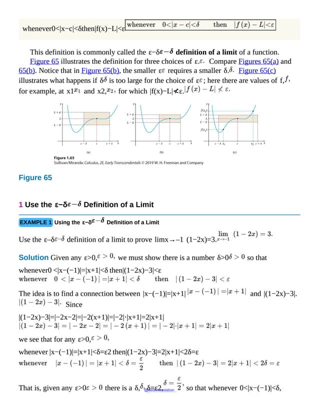
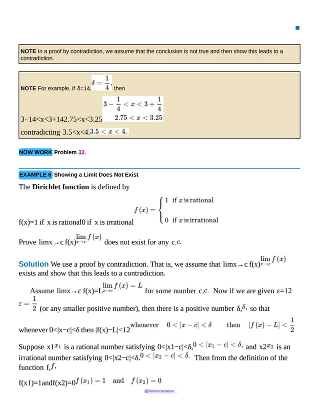
429. 51. Discuss limx→0 f(x) and limx→1 f(x) if
f(x)=x2 if x is rational0 if x is irrational
52. Discuss limx→0 f(x) if f(x)=x2 if x is rationaltan x if x is irrational
Challenge Problems
53. Use the ε -δ definition of limit to prove that limx→1 (4x3+3x2−24x+22)=5.
54. If limx→c f(x)=L and limx→c g(x)=M, prove that
limx→c [f(x)+g(x)]=L+M. Use the ε -δ definition of
limit.
55. For limx→∞ 2−x5+4x2=−12, find a value of M that satisfies
the ε -δ definition of a limit at infinity for ε=0.01.
56. Use the ε -δ definition of a limit to prove that the linear function f(x)=ax+b
is continuous for all real numbers.
57. Show that the function f(x)=0 if x is rationalx if x is irrational
is continuous only at x=0.
58. Suppose that f is defined on an interval (a,b) and there is a number K so that
f(x)−f(c)≤K|x−c|
for all c in (a,b) and x in (a,b). Such a constant K is called a Lipschitz constant. Find a
Lipschitz constant for f(x)=x3 on the interval (0,2).
1. = NOW WORK problem
= Graphing technology recommended
= Computer Algebra System recommended
@Seismicisolation
@Seismicisolation

430. @Seismicisolation
@Seismicisolation

431. Chapter Review
THINGS TO KNOW
1.1 Limits of Functions Using Numerical and Graphical Techniques
Slope of a secant line: msec=f (x)−f (c)x−c (p. 79)
Slope of a tangent line: mtan=limx→c f (x)−f (c)x−c (p. 79)
limx→c f (x)=L: read, “The limit as x approaches c of f (x) is
equal to the number L.” (p. 80)
limx→c f (x)=L: interpreted as, “The value f (x) can be made as
close as we please to L, for x sufficiently close to c, but not equal to c. ” (p.
80)
One-sided limits (p. 81)
The limit L of a function y=f (x) as x approaches a number c does not
depend on the value of f at c. (p. 83)
The limit L of a function y=f (x) as x approaches a number c is unique.
A function cannot have more than one limit as x approaches c. (p. 83)
Theorem
The limit L of a function y=f (x) as x approaches a number c exists if and only
if both one-sided limits exist at c and both one-sided limits are equal. That is,
limx→c f (x)=L if and only if limx→c− f (x)=limx→c+ f (x)=L.
(p. 84)
1.2 Limits of Functions Using Properties of Limits
Basic Limits
limx→c A=A, A a constant, for any real number c. (p. 90)
@Seismicisolation
@Seismicisolation

432. limx→c x=c, for any real number c. (p. 90)
Properties of Limits If f and g are functions for which limx→c f (x) and
limx→c g (x) both exist and if k is any real number, then:
limx→c [f (x)±g (x)]=limx→c f (x)±limx→c g (x)
(pp. 91)
limx→c [f (x)⋅g (x)]=limx→c f (x)⋅limx→c g (x)
(p. 91)
limx→c [kg (x)]=k limx→c g (x) (p. 92)
limx→c [f (x)]n=limx→c f (x)n, n is a positive integer (p.
93)
limx→c f (x)n=limx→c f (x)n, where n≥2 is an integer,
provided f (x)>0 if n is even (p. 94)
limx→c [f (x)]m⁄n=limx→c f (x)m⁄n, provided
[f (x)]m⁄n is defined for positive integers m and n (p. 94)
limx→c f (x)g (x)=limx→c f (x)limx→c g (x), provided
limx→c g (x)≠0 (p. 96)
If P is a polynomial function, then limx→c P (x)=P (c). (p. 95)
If R is a rational function and if c is in the domain of R, then
limx→c R (x)=R (c). (p. 96)
1.3 Continuity
Definitions
Continuity at a number (p. 102)
Removable discontinuity (p. 104)
@Seismicisolation
@Seismicisolation

433. One-sided continuity at a number (p. 104)
Continuity on an interval (p. 105)
Properties of Continuity
A polynomial function is continuous on its domain, all real numbers. (p. 106)
A rational function is continuous on its domain. (p. 106)
If the functions f and g are continuous at a number c, and if k is a real number,
then the functions f+g, f−g, f⋅g, and kf are also continuous at c.
If g (c)≠0, the function fg is continuous at c. (p. 107)
If a function g is continuous at c and a function f is continuous at g (c), then
the composite function (f∘g) (x)=f (g (x)) is continuous at c.
(p. 108)
If f is a one-to-one function that is continuous on its domain, then its inverse function
f−1 is also continuous on its domain. (p. 108)
The Intermediate Value Theorem Let f be a function that is continuous on a closed
interval [a,b] and f (a)≠f (b). If N is any number between f (a) and
f (b), then there is at least one number c in the open interval (a,b) for which
f (c)=N. (p. 109)
1.4 Limits and Continuity of Trigonometric, Exponential, and Logarithmic Functions
Basic Limits
limθ→0 sin θθ=1 (p. 117)
limθ→0 cos θ−1θ=0 (p. 119)
limx→c sin x=sin c (p. 120)
limx→c cos x=cos c (p. 120)
limx→c ax=ac; a>0, a≠1 (p. 122)
limx→c logax=logac; c>0, a>0, a≠1 (p. 122)
@Seismicisolation
@Seismicisolation

434. Squeeze Theorem If the functions f, g, and h have the property that for all x in an
open interval containing c, except possibly at c, f (x)≤g (x)≤h (x),
and if limx→c f (x)=limx→c h (x)=L, then limx→c g (x)=L.
(p. 115)
Properties of Continuity
The six trigonometric functions are continuous on their domains. (p. 120)
The six inverse trigonometric functions are continuous on their domains. (p. 121)
An exponential function is continuous for all real numbers. (p. 122)
A logarithmic function is continuous for all positive real numbers. (p. 122)
1.5 Infinite Limits; Limits at Infinity; Asymptotes
Basic Limits
limx→0− 1x=−∞ (p. 125)
limx→0+ 1x=∞ (p. 125)
limx→0 1x2=∞ (p. 125)
limx→0+ ln x=−∞ (p. 126)
limx→∞ 1x=0 (p. 129)
limx→−∞ 1x=0 (p. 129)
limx→−∞ ex=0 (p. 133)
limx→∞ ex=∞ (p. 133)
limx→∞ ln x=∞ (p. 133)
Definitions
Vertical asymptote (p. 128)
Horizontal asymptote (p. 135) @Seismicisolation
@Seismicisolation

435. Properties of Limits at Infinity (p. 129): If k is a real number, n≥2 is an integer,
and the functions f and g approach real numbers as x→∞, then:
limx→∞ A=A, where A is a constant
limx→∞ [kf (x)]=klimx→∞ f (x)
limx→∞ [f (x)±g (x)]=limx→∞ f (x)±limx→∞ g (x)
limx→∞ [f (x)g (x)]=limx→∞ f (x)limx→∞ g (x)
limx→∞ f (x)g (x)=limx→∞ f (x)limx→∞ g (x) provided
limx→∞ g (x)≠0
limx→∞ [f (x)]n=limx→∞ f (x)n
limx→∞ f (x)n=limx→∞ f (x)n, where f (x)>0 if
n is even
limx→±∞ kxp=0, p>0, provided xp is defined when x<0
limx→∞ xn=∞,n>0, an integer (p. 131)
limx→−∞ xn=∞ if n is a positive, even integer
limx→−∞ xn=−∞ if n is a positive, odd integer (p. 131)
For a polynomial function
p (x)=anxn+⋯+a0,an≠0
limx→±∞ p (x)=limx→±∞ anxn (p. 131)
The limit at infinity of R (x)=p (x)q (x) (p. 132)
@Seismicisolation
@Seismicisolation

436. 1.6 The ε−δ Definition of a Limit
Definitions
Limit of a Function (p. 141)
Limit at Infinity (p. 146)
Infinite Limit (p. 146)
Infinite Limit at Infinity (p. 147)
Properties of limits
If limx→c f (x)>0, then there is an open interval around c, for which
f (x)>0 everywhere in the interval, except possibly at c. (p. 145)
If limx→c f (x)<0, then there is an open interval around c, for which
f (x)<0 everywhere in the interval, except possibly at c. (p. 146)
OBJECTIVES
Section You should be able to … Examples Review Exercises
1.1 1 Discuss the idea of a limit (p. 80) 1 4
2 Investigate a limit using a table (p. 80) 2–4 1
3 Investigate a limit using a graph (p. 82) 5–8 2, 3
1.2 1 Find the limit of a sum, a difference, and a product (p. 91) 1–6 8, 10, 12, 14, 22, 26,
29, 30, 47, 48
2 Find the limit of a power and the limit of a root (p. 93) 7–9 11, 18, 28, 55
3 Find the limit of a polynomial (p. 95) 10 10, 22
4 Find the limit of a quotient (p. 96) 11–14 13–17, 19–21, 23–25,
27, 56
5 Find the limit of an average rate of change (p. 98) 15 37
6 Find the limit of a difference quotient (p. 98) 16 5, 6, 49
1.3 1 Determine whether a function is continuous at a number (p. 102) 1–4 31–36
2 Determine intervals on which a function is continuous (p. 105) 5, 6 39–42
3 Use properties of continuity (p. 107) 7, 8 39–42
4 Use the Intermediate Value Theorem (p. 109) 9, 10 38, 44–46
1.4 1 Use the Squeeze Theorem to find a limit (p. 115) 1 7, 69
2 Find limits involving trigonometric functions (p. 116) 2, 3 9, 51–55
3 Determine where the trigonometric functions are continuous (p.
120)
4 63–65
4 Determine where an exponential or a logarithmic function is
continuous (p. 121)
5 43
1.5 1 Find infinite limits (p. 125) 1–3 57, 58
2 Find the vertical asymptotes of a graph (p. 128) 4 61, 62
3 Find limits at infinity (p. 128) 5–11 59, 60
4 Find the horizontal asymptotes of a graph (p. 135) 12 61, 62
@Seismicisolation
@Seismicisolation

437. 5 Find the asymptotes of the graph of a rational function (p. 135) 13 61, 68
1.6 1 Use the ε−δ definition of a limit (p. 141) 1–7 50, 66
REVIEW EXERCISES
1. Use a table of numbers to investigate limx→0 1−cos x1+cos x.
In Problems 2 and 3, use a graph to investigate limx→c f (x).
2. f (x)=2x−5 if x<16−9x if x≥1 at c=1
3. f (x)=x2+2 if x<22x+1 if x≥2 at c=2
4. Write the statement “f (x) can be made as close as we please to 5 by choosing x
sufficiently close to, but not equal to, 3” symbolically.
In Problems 5 and 6, for each function find the limit of the difference quotient
limh→0 f (x+h)−f (x)h.
5. f (x)=3x
6. f (x)=3x2+2x
7. Find limx→0 f (x) if 1+sin x≤f (x)≤|x|+1
In Problems 8–22, find each limit.
8. limx→2 2x−1x
9. limx→π x cos x
10. limx→−1 x3+3x2−x−1
11. limx→0 x (x+2)33
12. limx→0 [ (2x+3) (x5+5x)] @Seismicisolation
@Seismicisolation

438. 13. limx→3 x3−27x−3
14. limx→3 x2x−3−3xx−3
15. limx→2 x2−4x−2
16. limx→−1 x2+3x+2x2+4x+3
17. limx→−2 x3+5x2+6xx2+x−2
18. limx→1 x2−3x+1x15
19. limx→2 3−x2+5x2−4
20. limx→0 1x 1 (2+x)2−14
21. limx→0 x+32−9x
22. limx→1 [ (x3−3x2+3x−1) (x+1)2]
In Problems 23–28, find each one-sided limit, if it exists.
23. limx→−2+ x2+5x+6x+2
24. limx→5+ |x−5|x−5
25. limx→1− |x−1|x−1
26. limx→3⁄2+ ⌊2x⌋
@Seismicisolation
@Seismicisolation

439. 27. limx→4− x2−16x−4
28. limx→1+ x−1
In Problems 29 and 30, find limx→c− f (x) and limx→c+ f (x) for the
given c . Determine whether limx→c f (x) exists.
29. f (x)=2x+3 if x<29−x if x≥2 at c=2
30. f (x)=3x+1 if x<310 if x=34x−2 if x>3 at c=3
In Problems 31–36, determine whether f is continuous at c.
31. f (x)=5x−2 if x<15 if x=12x+1 if x>1 at c=1
32. f (x)=x2 if x<−12 if x=−1−3x−2 if x>−1 at c=−1
33. f (x)=4−3x2 if x<04 if x=016−x2 if 0<x≤4 at c=0
@Seismicisolation
@Seismicisolation

440. 34. f (x)=4+x if−4≤x≤4x2−16x−4 if x>4 at c=4
35. f (x)=⌊2x⌋ at c=12
36. f (x)=|x−5| at c=5
37. a. Find the average rate of change of f (x)=2x2−5x from 1 to x.
b. Find the limit as x approaches 1 of the average rate of change found in (a).
38. A function f is defined on the interval [−1,1] with the following properties: f
is continuous on [−1,1] except at 0, negative at −1, positive at 1, but with
no zeros. Does this contradict the Intermediate Value Theorem?
In Problems 39–43 find all numbers x for which f is continuous.
39. f (x)=xx3−27
40. f (x)=x2−3x2+5x+6
41. f (x)=2x+1x3+4x2+4x
42. f (x)=x−1
43. f (x)=2−x
44. Use the Intermediate Value Theorem to determine whether 2x3+3x2−23x−42=0
has a zero in the interval [3,4].
In Problems 45 and 46, use the Intermediate Value Theorem to approximate the zero correct
to three decimal places.
45. f (x)=8x4−2x2+5x−1 on the interval 0,1.
46. f (x)=3x3−10x+9; zero between −3 and −2.
47. Find limx→0+ | x |x (1−x) and limx→0− | x |x (1−x).
@Seismicisolation
@Seismicisolation

441. What can you say about limx→0 | x |x (1−x) ?
48. Find limx→2 x2x−2−2xx−2. Then comment on the statement
that this limit is given by limx→2 x2x−2−limx→2 2xx−2.
49. Find limh→0 f (x+h)−f (x)h for f (x)=x.
50. For limx→3 (2x+1)=7, find the largest possible δ that “works” for
ε=0.01.
In Problems 51–60, find each limit.
51. limx→0 cos (tan x)
52. limx→0 sin x4x
53. limx→0 tan (3x)tan (4x)
54. limx→0 cos x3−1x
55. limx→0 cos x−1x10
56. limx→0 e4x−1ex−1
57. limx→π⁄2+ tan x
58. limx→−3 2+x (x+3)2
59. limx→∞ 3x3−2x+1x3−8
@Seismicisolation
@Seismicisolation

442. 60. limx→∞ 3x4+x2x2
In Problems 61 and 62, find any vertical and horizontal asymptotes of f.
61. f (x)=4x−2x+3
62. f (x)=2xx2−4
63. Let f (x)=tan x2x if x≠012 if x=0. Is f continuous at 0 ?
64. Let f (x)=sin (3x)x if x≠01 if x=0. Is f continuous at 0 ?
65. The function f (x)=cosπx+π2x is not defined at 0. Decide how to
define f (0) so that f is continuous at 0.
66. Use the ε−δ definition of a limit to prove limx→−3 (x2−9)≠18.
67. a. Sketch a graph of a function f that has the following properties:
f (−1)=0 limx→∞ f (x)=2 limx→−∞ f (x)=2limx→4− f (x)=−∞ limx→4+ f (x)=∞
b. Define a function that describes your graph.
68. a. Find the domain and the intercepts (if any) of
R (x)=2x2−5x+25x2−x−2.
b. Discuss the behavior of the graph of R at numbers where R is not defined.
c. Find any vertical or horizontal asymptotes of the function R.
69. If 1−x2≤f (x)≤cos x for all x in the interval −π2<x<π2,
@Seismicisolation
@Seismicisolation

443. show that limx→0 f (x)=1.
@Seismicisolation
@Seismicisolation

444. CHAPTER 1 PROJECT Pollution in Clear Lake
The Toxic Waste Disposal Company (TWDC) specializes in the disposal of a particularly
dangerous pollutant, Agent Yellow (AY). Unfortunately, instead of safely disposing of this
pollutant, the company simply dumped AY in (formerly) Clear Lake. Fortunately, they
have been caught and are now defending themselves in court.
The facts below are not in dispute. As a result of TWDC’s activity, the current
concentration of AY in Clear Lake is now 10 ppm (parts per million). Clear Lake is part of
a chain of rivers and lakes. Fresh water flows into Clear Lake and the contaminated water
flows downstream from it. The Department of Environmental Protection estimates that the
level of contamination in Clear Lake will fall by 20% each year. These facts can be
modeled as
p(0)=10 p(t+1)=0.80p(t)
where p=p(t), measured in ppm, is the concentration of pollutants in the lake at
time t, in years.
1. Explain how the above equations model the facts.
2. Create a table showing the values of t for t=0,1,2,…,20.
3. Show that p(t)=10(0.8)t.
4. Use technology to graph p=p(t).
@Seismicisolation
@Seismicisolation

445. 5. What is limx→∞ p(t) ?
Lawyers for TWDC looked at the results in 1–5 above and argued that their client has not
done any real damage. They concluded that Clear Lake would eventually return to its
former clear and unpolluted state. They even called in a mathematician, who wrote the
following on a blackboard:
limt→∞ p(t)=0
and explained that this bit of mathematics means, descriptively, that after many years the
concentration of AY will, indeed, be close to zero.
Concerned citizens booed the mathematician’s testimony. Fortunately, one of them has
taken calculus and knows a little bit about limits. She noted that, although “after many
years the concentration of AY will approach zero,” the townspeople like to swim in Clear
Lake and state regulations prohibit swimming unless the concentration of AY is below 2
ppm. She proposed a fine of $100,000 per year for each full year that the lake is unsafe for
swimming. She also questioned the mathematician, saying, “Your testimony was correct as
far as it went, but I remember from studying calculus that talking about the eventual
concentration of AY after many, many years is only a small part of the story. The more
precise meaning of your statement limt→∞ p(t)=0 is that given some
tolerance T for the concentration of AY, there is some time N (which may be very far
in the future) so that for all t>N, p(t)<T. ”
6. Using a table or a graph for p=p(t), find N so that if t>N, then p(t)
<2.
7. How much is the fine?
Her words were greeted by applause. The town manager sprang to his feet and noted that
although a tolerance of 2 ppm was fine for swimming, the town used Clear Lake for its
drinking water and until the concentration of AY dropped below 0.5 ppm, the water would
be unsafe for drinking. He proposed a fine of $200,000 per year for each full year the
water was unfit for drinking.
8. Using a table or a graph for p=p(t), find N so that if t>N, then p(t)
<0.5.
9. How much is the fine?
10. How would you find if you were on the jury trying TWDC? If the jury found TWDC
guilty, what fine would you recommend? Explain your answers.
@Seismicisolation
@Seismicisolation

446. 2 The Derivative
2.1 Rates of Change and the Derivative
2.2 The Derivative as a Function
2.3 The Derivative of a Polynomial Function; The Derivative of y=ex
2.4 Differentiating the Product and the Quotient of Two Functions; Higher-Order Derivatives
2.5 The Derivative of the Trigonometric Functions
Chapter Review
Chapter Project
The Apollo Lunar Module
“One Giant Leap for Mankind”
On May 25, 1961, in a special address to Congress, U.S. President John F.
Kennedy proposed the goal “before this decade is out, of landing a man on the
Moon and returning him safely to the Earth.” Roughly eight years later, on July 16,
1969, a Saturn V rocket launched from the Kennedy Space Center in Florida,
carrying the Apollo 11 spacecraft and three astronauts—Neil Armstrong, Buzz
Aldrin, and Michael Collins—bound for the Moon.
The Apollo spacecraft had three parts: the Command Module with a cabin for
@Seismicisolation
@Seismicisolation

447. the three astronauts; the Service Module that supported the Command Module
with propulsion, electrical power, oxygen, and water; and the Lunar Module for
landing on the Moon. After its launch, the spacecraft traveled for three days until it
entered into lunar orbit. Armstrong and Aldrin then moved into the Lunar Module,
which they landed in the flat expanse of the Sea of Tranquility. After more than 21
hours, the first humans to touch the surface of the Moon crawled into the Lunar
Module and lifted off to rejoin the Command Module, which Collins had been
piloting in lunar orbit. The three astronauts then headed back to Earth, where they
splashed down in the Pacific Ocean on July 24.
CHAPTER 2 PROJECT In the Chapter Project on page 206 at the end of this
chapter, we explore some of the physics at work that allowed engineers and pilots
to successfully maneuver the Lunar Module to the Moon’s surface.
Chapter 2 opens by returning to the tangent problem to find an equation of the tangent line to
the graph of a function f at a point P=(c,f(c)). Remember in Section 1.1 we
found that the slope of a tangent line was a limit,
mtan=limx→c f(x)−f(c)x−c
This limit turns out to be one of the most significant ideas in calculus, the derivative.
In this chapter, we introduce interpretations of the derivative, treat the derivative as a
function, and consider some properties of the derivative. By the end of the chapter, you will
have a collection of basic derivative formulas and derivative rules that will be used
throughout your study of calculus.
@Seismicisolation
@Seismicisolation

448. (1)
2.1 Rates of Change and the Derivative
OBJECTIVES When you finish this section, you should be able to:
1 Find equations for the tangent line and the normal line to the graph of a
function
2 Find the rate of change of a function
3 Find average velocity and instantaneous velocity
4 Find the derivative of a function at a number
In Chapter 1 we discussed the tangent problem: Given a function f and a point P on its graph,
what is the slope of the tangent line to the graph of f at P? See Figure 1, where ℓT is the
tangent line to the graph of f at the point P=(c,f(c)).
Figure 1 msec= slope of the secant line.
The tangent line ℓT to the graph of f at P must contain the point P. Since
finding the slope requires two points, and we have only one point on the tangent line ℓT,
we reason as follows.
Suppose we choose any point Q=(x,f(x)), other than P, on the graph of
f. (Q can be to the left or to the right of P ; we chose Q to be to the right of P. )
The line containing the points P=(c,f(c)) and Q=(x,f(x)) is a
secant line of the graph of f. The slope msec of this secant line is
@Seismicisolation
@Seismicisolation

449. msec=f(x)−f(c)x−c
Figure 2 mtan=limx→c f(x)−f(c)x−c
The
secant
lines
l1,
l2
and
l3
join
the
point
P
passing
through
the
points
Q1,
Q2,
and
Q3
Figure 2 shows three different points Q1, Q2, and Q3 on the graph of f that
are successively closer to the point P, and three associated secant lines ℓ1, ℓ2, and
ℓ3. The closer the points Q are to the point P, the closer the secant lines are to the
tangent line ℓT. The line ℓT, the limiting position of these secant lines, is the tangent
line to the graph of f at P.
If the limiting position of the secant lines is the tangent line, then the limit of the slopes
of the secant lines should equal the slope of the tangent line. Notice in Figure 2 that as the
points Q1, Q2, and Q3 move closer to the point P, the numbers x get closer
to c. So, equation (1) suggests that
mtan=Slope of the tangent line to f at P=Limit of f (x)−f (c)x−c as x gets closer
to c=limx→c f (x)−f (c)x−c
provided the limit exists.
DEFINITION Tangent Line
@Seismicisolation
@Seismicisolation

450. (2)
(3)
The tangent line to the graph of f at a point P is the line containing the point P=c,f (c)
and having the slope
mtan=limx→c f (x)−f (c)x−c
provided the limit exists.
NOTE It is possible for the limit in (2) not to exist. The geometric significance of this is discussed in the next
section.
The limit in equation (2) that defines the slope of the tangent line occurs so frequently
that it is given a special notation f′(c), read, “f prime of c, ” and called prime
notation:
f′(c)=limx→c f (x)−f (c)x−c
1 Find Equations for the Tangent Line and the Normal Line to the Graph of a
Function
THEOREM Equation of a Tangent Line
If mtan=f′(c) exists, then an equation of the tangent line to the graph of a
function y=f (x) at the point P=(c,f (c)) is
y−f (c)=f′(c) (x−c)
The line perpendicular to the tangent line at a point P on the graph of a function f is
called the normal line to the graph of f at P.
An equation of the normal line to the graph of a function y=f (x) at the point P=
(c,f (c)) is
y−f (c)=−⁢1f′(c)(x−c)
provided f′(c) exists and is not equal to zero. If f′(c)=0, the tangent line is
horizontal, the normal line is vertical, and the equation of the normal line is x=c.
@Seismicisolation
@Seismicisolation

451. RECALL Two lines, neither of which are horizontal, with slopes m1 and m2, respectively, are
perpendicular if and only if
m1=−1m2
EXAMPLE 1 Finding Equations for the Tangent Line and the Normal Line
a. Find the slope of the tangent line to the graph of f(x)=x2 at c=−2.
b. Use the result from (a) to find an equation of the tangent line when c=−2.
c. Find an equation of the normal line to the graph of f at the point (−2,4 ).
d. Graph f, the tangent line to f at (−2,4 ), and the normal line to f at (−2,4 )
on the same set of axes.
RECALL One way to find the limit of a quotient when the limit of the denominator is 0 is to factor the numerator
and divide out common factors.
Solution a. At c=−2, the slope of the tangent line is
f′(−2)=limx→−2 f(x)−f(−2)x−(−2)=limx→−2 x2−(−2)2x+2=limx→−2 x2−4x+2=limx→
−2 (x−2)=−4
NEED TO REVIEW? The point-slope form of a line is discussed in Appendix A.3, p. A-19.
b. We use the result from (a) and the point-slope form of an equation of a line to obtain an
equation of the tangent line. An equation of the tangent line containing the point (−2,f(−2))=
(−2,4) is
y−f(−2)=f′(−2)[x−(−2)]Point-slope form of an equation of the tangent line.y−4=
−4⋅(x+2)f(−2)=4;f′(−2)=−4y=−4x−4Simplify.
c. Since the slope of the tangent line to f at (−2,4 ) is −4, the slope of the normal
@Seismicisolation
@Seismicisolation

452. line to f at (−2,4 ) is 14.
Using the point-slope form of an equation of a line, an equation of the normal line is
y−4=14(x+2)y=14 x+92
d. The graphs of f, the tangent line to the graph of f at the point (−2,4 ), and the
normal line to the graph of f at (−2,4 ) are shown in Figure 3.
▪
Figure 3 f(x)=x2
NOW WORK Problem 11.
2 Find the Rate of Change of a Function
Everything in nature changes. Examples include climate change, change in the phases of the
Moon, and change in populations. To describe natural processes mathematically, the ideas of
change and rate of change are often used.
Recall that the average rate of change of a function y=f(x) over the interval
from c to x is given by
Average rate of change=f(x)−f(c)x−cx≠c
@Seismicisolation
@Seismicisolation

453. DEFINITION Instantaneous Rate of Change
The instantaneous rate of change of f at c is the limit as x approaches c of the
average rate of change. Symbolically, the instantaneous rate of change of f at c is
limx→c f(x)−f(c)x−c
provided the limit exists.
The expression “instantaneous rate of change” is often shortened to rate of change. Using
prime notation, the rate of change of f at c is f′(c)=limx→c f(x)−f(c)x−c.
EXAMPLE 2 Finding a Rate of Change
Find the rate of change of the function f(x)=x2−5x at:
a. c=2
b. Any real number c
Solution a. For c=2,
f(x)=x2−5xandf(2)=22−5⋅2=−6
The rate of change of f at c=2 is
f′(2)=limx→2 f(x)−f(2)x−2=limx→2 (x2−5x)−(−6)x−2=limx→2 x2−5x+6x−2=limx→2 (x
−2)(x−3)x−2=limx→2 x−3=−1
b. If c is any real number, then f(c)=c2−5c, and the rate of change of f at c
is
f′(c)=limx→c f(x)−f(c)x−c=limx→c (x2−5x)−(c2−5c)x−c=limx→c (x2−c2)−5(x−c)x
−c=limx→c (x−c)(x+c)−5(x−c)x−c=limx→c (x−c)(x+c−5)x−c=limx→c (x+c−5)=2c−5
@Seismicisolation
@Seismicisolation

454. ▪
NOW WORK Problem 17.
EXAMPLE 3 Finding the Rate of Change in a Biology Experiment
In a metabolic experiment, the mass M of glucose decreases according to the function
M(t)=4.5−0.03t2
where M is measured in grams (g) and t is the time in hours (h). Find the reaction rate M
′(t) at t=1 h.
Solution The reaction rate at t=1 is M′(1).
M′(1)=limt→1 M(t)−M(1)t−1=limt→1 (4.5−0.03t2)−(4.5−0.03)t−1=limt→1 −0.03t2+0.03t
−1=limt→1 (−0.03)(t2−1)t−1=limt→1 (−0.03)(t−1)(t+1)t−1=−0.03⋅2=−0.06
The reaction rate at t=1 h is −0.06 g/h. That is, the mass M of glucose at
t=1 h is decreasing at the rate of 0.06 g/h.
▪
NOW WORK Problem 43.
3 Find Average Velocity and Instantaneous Velocity
Average velocity is a physical example of an average rate of change. For example, consider
an object moving along a horizontal line with the positive direction to the right, or moving
along a vertical line with the positive direction upward. Motion along a line is referred to as
rectilinear motion. The object’s location at time t=0 is called its initial position. The
@Seismicisolation
@Seismicisolation

455. initial position is usually marked as the origin O on the line. See Figure 4. We assume the
position s at time t of the object from the origin is given by a function s=f(t).
Here s is the signed, or directed, distance (using some measure of distance such as
centimeters, meters, feet, etc.) of the object from O at time t (in seconds or hours). The
function f is usually called the position function of the object.
Figure 4 t is the travel time. s is the signed distance of the object from the origin at time
t.
DEFINITION Average Velocity
The signed distance s from the origin at time t of an object in rectilinear motion is given
by the position function s=f(t). If at time t0 the object is at s0=f(t0)
and at time t1 the object is at s1=f(t1), then the change in time is Δt=t1−t0
and the change in position is Δs=s1−s0=f(t1)−f(t0).
The average rate of change of position with respect to time
is
ΔsΔt=f(t1)−f(t0)t1−t0t1≠t0
and is called the average velocity of the object over the interval [t0,t1]. See Figure
5.
@Seismicisolation
@Seismicisolation

456. Figure 5 The average velocity is ΔsΔt.
EXAMPLE 4 Finding Average Velocity
The Mike O'Callaghan–Pat Tillman Memorial Bridge spanning the Colorado River opened
on October 16, 2010. Having a span of 1900 ft, it is the longest arch bridge in the Western
Hemisphere, and its roadway is 890 ft above the Colorado River.
If a rock falls from the roadway, the function s=f(t)=16t2 gives the
distance s, in feet, that the rock falls after t seconds for 0≤t≤7.458. Here
7.458 s is the approximate time it takes the rock to fall 890 ft into the river. The
average velocity of the rock during its fall is
ΔsΔt=f(7.458)−f(0)7.458−0=890−07.458≈119.335 ft/s ▪
NOTE Here the motion occurs along a vertical line with the positive direction downward.
@Seismicisolation
@Seismicisolation

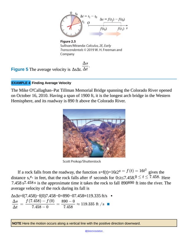
457. The average velocity of the rock in Example 4 approximates the average velocity over the
interval [0,7.458]. But the average velocity does not tell us about the velocity at
any particular instant of time. That is, it gives no information about the rock’s instantaneous
velocity.
We can investigate the instantaneous velocity of the rock, say, at t=3 s, by
computing average velocities for short intervals of time beginning at t=3. First we
compute the average velocity for the interval beginning at t=3 and ending at t=3.5.
The corresponding distances the rock has fallen are
f(3)=16⋅32=144 ftandf(3.5)=16⋅3.52=196 ft
Then Δt=3.5−3.0=0.5, and during this 0.5 -s interval,
Average velocity=ΔsΔt=f(3.5)−f(3)3.5−3=196−1440.5=104 ft/s
Table 1 shows average velocities of the rock for smaller intervals of time.
TABLE 1
Time
interval Start t0=3 End t Δt ΔsΔt=f(t)−f(t0)t−t0=16t2−144t−3
[3, 3.1] 3 3.1 0.1 ΔsΔt=f(3.1)−f(3)3.1−3=16⋅3.12−1440.1=97.6
[3, 3.01] 3 3.01 0.01 ΔsΔt=f(3.01)−f(3)3.01−3=16⋅3.012−1440.01=96.16
[3,
3.0001]
3 3.0001 0.0001 ΔsΔt=f(3.0001)−f(3)3.0001−3=16⋅3.00012−1440.0001=96.0016
The average velocity of 96.0016 over the time interval Δt=0.0001 s
should be very close to the instantaneous velocity of the rock at t=3 s. As Δt gets
closer to 0, the average velocity gets closer to the instantaneous velocity. So, to obtain the
instantaneous velocity at t=3 precisely, we use the limit of the average velocity as Δt
approaches 0 or, equivalently, as t approaches 3.
limΔt→0 ΔsΔt=limt→3 f(t)−f(3)t−3=limt→3 16t2−16⋅32t−3=limt→3 16(t2−9)t
−3=limt→3 16(t−3)(t+3)t−3=limt→3 [16(t+3)]=96
The rock’s instantaneous velocity at t=3 s is 96 ft/s.
We generalize this result to obtain a definition for instantaneous velocity.
DEFINITION Instantaneous Velocity
@Seismicisolation
@Seismicisolation

458. If s=f(t) is the position function of an object at time t, the instantaneous
velocity v of the object at time t0 is defined as the limit of the average velocity ΔsΔt
as Δt approaches 0. That is,
v=limΔt→0 ΔsΔt=limt→t0 f(t)−f(t0)t−t0
provided the limit exists.
We usually shorten “instantaneous velocity” and just use the word “velocity.”
NOW WORK Problem 31.
EXAMPLE 5 Finding Velocity
Find the velocity v of the falling rock from Example 4 at:
a. t0=1 s after it begins to fall
b. t0=7.4 s, just before it hits the Colorado River
c. At any time t0.
Solution a. Use the definition of instantaneous velocity with f(t)=16t2 and
t0=1.
v=limΔt→0 ΔsΔt=limt→1 f(t)−f(1)t−1=limt→1 16t2−16t−1=limt→1 16(t2−1)t
−1=limt→1 16(t−1)(t+1)t−1=limt→1 [16(t+1)]=32
At 1 s, the velocity of the rock is 32 ft/s.
b. For t0=7.4 s,
v=limΔt→0 ΔsΔt=limt→7.4 f(t)−f(7.4)t−7.4=limt→7.4 16t2−16⋅(7.4)2t
−7.4=limt→7.4 16[t2−(7.4)2]t−7.4=limt→7.4 16(t−7.4)(t+7.4)t
−7.4=limt→7.4 [16(t+7.4)]=16(14.8)=236.8
@Seismicisolation
@Seismicisolation

459. At 7.4 s, the velocity of the rock is 236.8 ft/s.
NOTE Did you know? 236.8 ft/s is more than 161 mi/h!
c.
v=limt→t0 f(t)−f(t0)t−t0=limt→t0 16t2−16t02t−t0=limt→t0 16(t−t0)(t+t0)t
−t0=16limt→t0 (t+t0)=32t0
At t0 seconds, the velocity of the rock is 32t0 ft/s. ▪
NOW WORK Problem 33.
4 Find the Derivative of a Function at a Number
Slope of a tangent line, rate of change of a function, and velocity are all found using the same
limit,
f′(c)=limx→c f(x)−f(c)x−c
The common underlying idea is the mathematical concept of derivative.
DEFINITION Derivative of a Function at a Number
If y=f(x) is a function and c is in the domain of f, then the derivative of f at
c, denoted by f′(c), is the number
f′(c)=limx→c f(x)−f(c)x−c
@Seismicisolation
@Seismicisolation

460. provided this limit exists.
EXAMPLE 6 Finding the Derivative of a Function at a Number
Find the derivative of f(x)=2x2−3x−2 at x=2. That is, find f′(2).
Solution Using the definition of the derivative, we have
f′(2)=limx→2 f(x)−f(2)x−2=limx→2 (2x2−3x−2)−0x−2f(2)=2⋅4−3⋅2−2=0=limx→2 (x−2)
(2x+1)x−2=limx→2 (2x+1)=5
▪
NOW WORK Problem 23.
So far we have given three interpretations of the derivative:
Geometric interpretation: If y=f(x), the derivative f′(c) is the slope of
the tangent line to the graph of f at the point (c,f(c)).
Rate of change of a function interpretation: If y=f(x), the derivative f′(c)
is the rate of change of f at c.
Physical interpretation: If the signed distance s from the origin at time t of an object
in rectilinear motion is given by the position function s=f(t), the derivative f
′(t0) is the velocity of the object at time t0.
EXAMPLE 7 Finding an Equation of a Tangent Line
a. Find the derivative of f(x)=2x at x=8.
b. Use the derivative f′(8) to find an equation of the tangent line to the graph of f at
the point (8,4).
@Seismicisolation
@Seismicisolation

461. Solution a. The derivative of f at 8 is
b. The slope of the tangent line to the graph of f at the point (8,4) is f′(8)=14.
Using the point-slope form of a line, we get
y−4=f′(8)(x−8) y−y1=m(x−x1)y−4=14 (x−8) f′(8)=14y=14 x+2
▪
The graphs of f and the tangent line to the graph of f at (8,4) are shown in Figure
6.
Figure 6
@Seismicisolation
@Seismicisolation

462. NOW WORK Problem 15.
EXAMPLE 8 Approximating the Derivative of a Function Defined by a Table
The table below lists several values of a function y=f(x) that is continuous on the
interval [−1,5 ] and has a derivative at each number in the interval (−1,5 ).
Approximate the derivative of f at 2.
x 0 1 2 3 4
f(x) 0 3 12 33 72
Solution There are several ways to approximate the derivative of a function defined by a
table. Each uses an average rate of change to approximate the rate of change of f at 2,
which is the derivative of f at 2.
Using the average rate of change from 2 to 3, we have
f(3)−f(2)3−2=33−121=21
With this choice, f′(2) is approximately 21.
Using the average rate of change from 1 to 2, we have
f(2)−f(1)2−1=12−31=9
With this choice, f′(2) is approximately 9.
A third approximation can be found by averaging the above two approximations. Then f
′(2) is approximately 21+92=15. ▪
NOW WORK Problem 51.
2.1 Assess Your Understanding
Concepts and Vocabulary
1. True or False The derivative is used to find instantaneous velocity.
2. True or False The derivative can be used to find the rate of change of a function.
3. The notation f′(c) is read f of c ; f′(c) represents the of
the tangent line to the graph of f at the point .
@Seismicisolation
@Seismicisolation

463. 4. True or False If it exists, limx→3 f(x)−f(3)x−3 is the derivative of
the function f at 3.
5. If f(x)=6x−3, then f′(3)= .
6. The velocity of an object, the slope of a tangent line, and the rate of change of a
function are three different interpretations of the mathematical concept called the
__________.
Skill Building
In Problems 7–16,
a. Find an equation for the tangent line to the graph of each function at the indicated
point.
b. Find an equation of the normal line to each function at the indicated point.
c. Graph the function, the tangent line, and the normal line at the indicated point on the
same set of coordinate axes.
7. f(x)=3x2 at (−2,12)
8. f(x)=x2+2 at (−1,3)
9. f(x)=x3 at (−2,−8)
10. f(x)=x3+1 at (1,2)
11. f(x)=1x at (1,1)
12. f(x)=x at (4,2)
13. f(x)=1x+5 at 1,16
14. f(x)=2x+4 at 1,25
15. f(x)=1x at (1,1)
16. f(x)=1x2 at (1,1)
@Seismicisolation
@Seismicisolation

464. In Problems 17–20, find the rate of change of f at the indicated numbers.
17. f(x)=5x−2 at (a) c=0, (b) c=2
18. f(x)=x2−1 at (a) c=−1, (b) c=1
19. f(x)=x2x+3 at (a) c=0, (b) c=1
20. f(x)=xx2−1 at (a) c=0, (b) c=2
In Problems 21–30, find the derivative of each function at the given number.
21. f(x)=2x+3 at 1
22. f(x)=3x−5 at 2
23. f(x)=x2−2 at 0
24. f(x)=2x2+4 at 1
25. f(x)=3x2+x+5 at −1
26. f(x)=2x2−x−7 at −1
27. f(x)=x at 4
28. f(x)=1x2 at 2
29. f(x)=2−5x1+x at 0
30. f(x)=2+3x2+x at 1
31. Approximating Velocity An object in rectilinear motion moves according to the
position function s(t)=10t2 (s in centimeters and t in seconds).
Approximate the velocity of the object at time t0=3 s by letting Δt first equal
0.1 s, then 0.01 s, and finally 0.001 s. What limit does the velocity appear
to be approaching? Organize the results in a table.
32. Approximating Velocity An object in rectilinear motion moves according to the
position function s(t)=5−t2 (s in centimeters and t in seconds).
Approximate the velocity of the object at time t0=1 by letting Δt first equal
0.1, then 0.01, and finally 0.001. What limit does the velocity appear to be approaching?
@Seismicisolation
@Seismicisolation

465. Organize the results in a table.
33. Rectilinear Motion As an object in rectilinear motion moves, its signed distance s (in
meters) from the origin after t seconds is given by the position function s=f(t)=3t2+4t.
Find the velocity v at t0=0. At t0=2. At any time
t0.
34. Rectilinear Motion As an object in rectilinear motion moves, its signed distance s (in
meters) from the origin after t seconds is given by the position function s=f(t)=2t3+4.
Find the velocity v at t0=0. At t0=3. At any time t0.
35. Rectilinear Motion As an object in rectilinear motion moves, its signed distance s
from the origin at time t is given by the position function s=s(t)=3t2−1t,
where s is in centimeters and t is in seconds. Find the velocity v
of the object at t0=1 and t0=4.
36. Rectilinear Motion As an object in rectilinear motion moves, its signed distance s
from the origin at time t is given by the position function s=s(t)=4t,
where s is in centimeters and t is in seconds. Find the velocity v of the object at
t0=1 and t0=4.
37. The Princeton Dinky is the shortest rail line in the country. It runs for 2.7 miles,
connecting Princeton University to the Princeton Junction railroad station. The Dinky
starts from the university and moves north toward Princeton Junction. Its distance from
Princeton is shown in the graph below, where the time t is in minutes and the distance
s of the Dinky from Princeton University is in miles.
a. When is the Dinky headed toward Princeton University?
b. When is it headed toward Princeton Junction?
@Seismicisolation
@Seismicisolation

466. c. When is the Dinky stopped?
d. Find its average velocity on a trip from Princeton to Princeton Junction.
e. Find its average velocity for the round trip shown in the graph, that is, from t=0
to t=13.
38. Barbara walks to the deli, which is six blocks east of her house. After walking two
blocks, she realizes she left her phone on her desk, so she runs home. After getting the
phone, and closing and locking the door, Barbara starts on her way again. At the deli,
she waits in line to buy a bottle of vitaminwaterTM, and then she jogs home. The graph
below represents Barbara’s journey. The time t is in minutes and s is Barbara’s
distance, in blocks, from home.
a. At what times is she headed toward the deli?
b. At what times is she headed home?
c. When is the graph horizontal? What does this indicate?
d. Find Barbara’s average velocity from home until she starts back to get her phone.
e. Find Barbara’s average velocity from home to the deli after getting her phone.
f. Find her average velocity from the deli to home.
@Seismicisolation
@Seismicisolation

467. Applications and Extensions
39. Slope of a Tangent Line An equation of the tangent line to the graph of a function f at
(2,6) is y=−3x+12. What is f′(2) ?
40. Slope of a Tangent Line An equation of the tangent line of a function f at (3,2)
is y=13 x+1. What is f′(3) ?
41. Tangent Line Does the tangent line to the graph of y=x2 at (1,1) pass
through the point (2,5) ?
42. Tangent Line Does the tangent line to the graph of y=x3 at (1,1) pass
through the point (2,5) ?
43. Respiration Rate A human being’s respiration rate R (in breaths per minute) is given
by R=R p=10.35+0.59p, where p is the partial pressure of
carbon dioxide in the lungs. Find the rate of change in respiration when p=50.
44. Instantaneous Rate of Change The volume V of the right circular cylinder of height
5 m and radius r m shown in the gure is V=V(r)=5πr2. Find the
instantaneous rate of change of the volume with respect to the radius when r=3 m.
45. Market Share During a month-long advertising campaign, the total sales S of a
magazine is modeled by the function S(x)=5x2+100x+10,000,
where x represents the number of days since the
campaign began, 0≤x≤30.
a. What is the average rate of change of sales from x=10 to x=20 days?
b. What is the instantaneous rate of change of sales when x=10 days?
@Seismicisolation
@Seismicisolation

468. 46. Demand Equation The demand equation for an item is p=p(x)=90−0.02x,
where p is the price in dollars and x is the number of units
(in thousands) made.
a. Assuming all units made can be sold, find the revenue function R(x)=xp(x).
b. Marginal Revenue Marginal revenue is defined as the additional revenue earned
by selling an additional unit. If we use R′(x) to measure the marginal
revenue, find the marginal revenue when 1 million units are sold.
47. Gravity If a ball is dropped from the top of the Empire State Building, 1002 ft
above the ground, the distance s (in feet) it falls after t seconds is s(t)=16t2.
a. What is the average velocity of the ball for the first 2 s?
b. How long does it take for the ball to hit the ground?
c. What is the average velocity of the ball during the time it is falling?
d. What is the velocity of the ball when it hits the ground?
48. Velocity A ball is thrown upward. Its height h in feet is given by h(t)=100t−16t2,
where t is the time elapsed in seconds.
a. What is the velocity v of the ball at t=0 s, t=1 s, and t=4 s ?
b. At what time t does the ball strike the ground?
c. At what time t does the ball reach its highest point?
(Hint: At the time the ball reaches its maximum height, it is stationary. So, its
velocity v=0. )
49. Gravity A rock is dropped from a height of 88.2 m and falls toward Earth in a straight
line. In t seconds the rock falls 4.9t2 m.
a. What is the average velocity of the rock for the first 2 s?
b. How long does it take for the rock to hit the ground?
c. What is the average velocity of the rock during its fall?
d. What is the velocity v of the rock when it hits the ground?
50. Velocity At a certain instant, the speedometer of an automobile reads V mi/h.
During the next 14 s the automobile travels 20 ft. Approximate V from this
information.
@Seismicisolation
@Seismicisolation

469. 51. A tank is filled with 80 l of water at 7 a.m. (t=0). Over the next 12 h the water
is continuously used. The table below gives the amount of water A(t) (in liters)
remaining in the tank at selected times t, where t measures the number of hours after
7 a.m.
t 0 2 5 7 9 12
A(t) 80 71 66 60 54 50
a. Use the table to approximate A′(5).
b. Using appropriate units, interpret A′(5) in the context of the problem.
52. The table below lists the outside temperature T, in degrees Fahrenheit, in Naples,
Florida, on a certain day in January, for selected times x, where x is the number of
hours since 12 a.m.
x 5 7 9 11 12 13 14 16 17
T(x) 62 71 74 78 81 83 84 85 78
a. Use the table to approximate T′(11).
b. Using appropriate units, interpret T′(11) in the context of the problem.
53. Rate of Change Show that the rate of change of a linear function f(x)=mx+b
is the slope m of the line y=mx+b.
54. Rate of Change Show that the rate of change of a quadratic function f(x)=ax2+bx+c
is a linear function of x.
55. Agriculture The graph represents the diameter d (in centimeters) of a maturing peach
as a function of the time t (in days) it is on the tree.
@Seismicisolation
@Seismicisolation

470. a. Interpret the derivative d′(t) as a rate of change.
b. Which is larger, d′(1) or d′(20)?
c. Interpret both d′(1) and d′(20).
56. Business The graph represents the demand d (in gallons) for olive oil as a function of
the cost c (in dollars per gallon) of the oil.
a. Interpret the derivative d′(c).
b. Which is larger, d′(5) or d′(30)? Give an interpretation to d′(5)
and d′(30).
57. Volume of a Cube A metal cube with eachedge of length x centimeters is expanding
uniformly as a consequence of being heated.
a. Find the average rate of change of the volume of the cube with respect to an edge
as x increases from 2.00 to 2.01 cm.
@Seismicisolation
@Seismicisolation

471. b. Find the instantaneous rate of change of the volume of the cube with respect to an
edge at the instant when x=2 cm.
@Seismicisolation
@Seismicisolation

472. (1)
(2)
2.2 The Derivative as a Function
OBJECTIVES When you finish this section, you should be able to:
1 Define the derivative function
2 Graph the derivative function
3 Identify where a function has no derivative
1 Define the Derivative Function
The derivative of f at a real number c has been defined as the real number
f′(c)=limx→c f (x)−f (c)x−c
provided the limit exists.
Another way to find the derivative of f at any real number is obtained by rewriting the
expression f (x)−f (c)x−c and letting x=c+h, h≠0. Then
f (x)−f (c)x−c=f (c+h)−f (c)(c+h)−c=f (c+h)−f (c)h
Since x=c+h, then as x approaches c , h approaches 0 . Equation (1) with
these changes becomes
f′(c)=limx→c f (x)−f (c)x−c=limh→0 f (c+h)−f (c)h
So, we have the following alternate form for the derivative of f at a real number c .
f′(c)=limh→0 f (c+h)−f (c)h
See Figure 7.
@Seismicisolation
@Seismicisolation

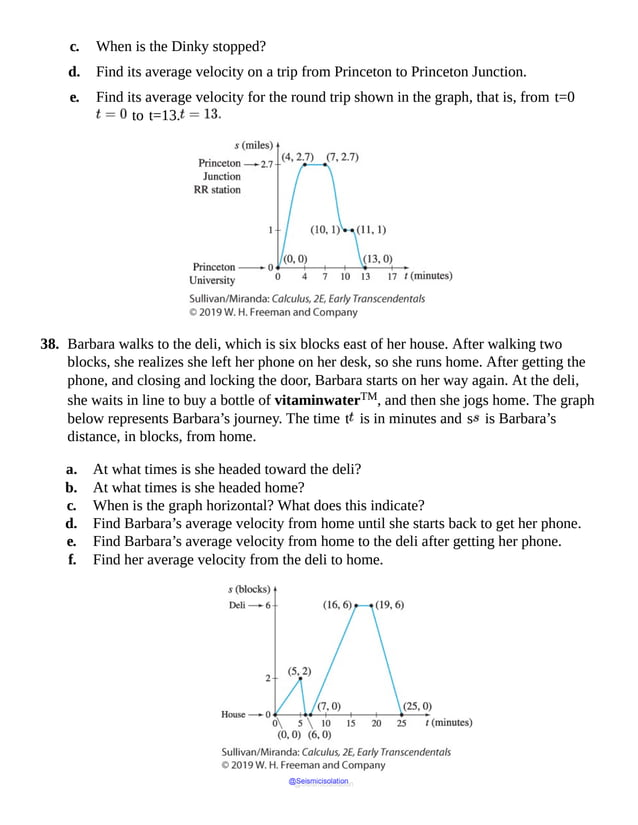
473. Figure 7 The slope of the tangent line at c is f′(c)=limh→0 f (c+h)−f (c)h
EXAMPLE 1 Finding the Derivative of a Function at a Number c
Find the derivative of the function f (x)=x2−5x at any real number c using
Form (2).
Solution Using Form (2), we have
f′(c)=limh→0 f (c+h)−f (c)h=limh→0 [(c+h)2−5(c+h)]−(c2−5c)h=limh→0 [(c2+2ch+h2)−5c
−5h]−c2+5ch=limh→0 2ch+h2−5hh=limh→0 h(2c+h−5)h=limh→0 (2c+h−5)=2c−5
▪
NOTE Compare the solution and answer found in Example 1 to Example 2(b) on p. 156.
Based on Example 1, if f (x)=x2−5x, then f′(c)=2c−5 for
@Seismicisolation
@Seismicisolation

474. (3)
any choice of c . That is, the derivative f′ is a function and, using x as the independent
variable, we can write f′(x)=2x−5.
DEFINITION The Derivative Function f′
The derivative function f′ of a function f is
f′(x)=limh→0 f (x+h)−f (x)h
provided the limit exists. If f has a derivative, then f is said to be differentiable.
IN WORDS In Form (3) the derivative is the limit of a difference quotient.
The domain of the function f′ is the set of real numbers in the domain of f for which
the limit (3) exists. So the domain of f′ is a subset of the domain of f .
We can use either Form (1) or Form (3) to find derivatives. However, if we want the
derivative of f at a specified number c , we usually use Form (1) to find f′(c). If we
want to find the derivative function of f , we usually use Form (3) to find f′(x). In this
section, we use the definitions of the derivative, Forms (1) and (3), to investigate derivatives.
In the next section, we begin to develop formulas for finding the derivatives.
EXAMPLE 2 Finding the Derivative Function
Differentiate f (x)=x and determine the domain of f′.
NOTE The instruction “differentiate f ” means “find the derivative of f .”
Solution The domain of f is {x|x≥0}. To find the derivative of f , we use
Form (3). Then
f′(x)=limh→0 f (x+h)−f (x)h=limh→0 x+h−xh
We rationalize the numerator to find the limit.
f′(x)=limh→0 x+h−xh⋅x+h+xx+h+x=limh→0 (x+h)
−xhx+h+x=limh→0 hhx+h+x=limh→0 1x+h+x=12x
@Seismicisolation
@Seismicisolation

475. The limit does not exist when x=0. But for all other x in the domain of f , the
limit does exist. So, the domain of the derivative function f′(x)=12x is
{x|x>0}. ▪
In Example 2, notice that the domain of the derivative function f′ is a proper subset of
the domain of the function f . The graphs of both f and f′ are shown in Figure 8.
Figure 8
NOW WORK Problem 15.
EXAMPLE 3 Interpreting the Derivative as a Rate of Change
The surface area S (in square meters) of a balloon is expanding as a function of time t (in
seconds) according to S=S(t)=5t2. Find the rate of change of the surface
area of the balloon with respect to time. What are the units of S′(t) ?
Solution An interpretation of the derivative function S′(t) is the rate of change of
S=S(t).
@Seismicisolation
@Seismicisolation

476. S′(t)=limh→0 S(t+h)
−S(t)h=limh→0 5(t+h)2−5t2hForm(3)=limh→0 5(t2+2th+h2)−5t2h=limh→0 5t2+10th+5h2−5
Since S′(t) is the limit of the quotient of a change in area divided by a change in time,
the units of the rate of change are square meters per second (m2⁄s). The rate of
change of the surface area S of the balloon with respect to time is 10t m2⁄s.
▪
NOW WORK Problem 67.
2 Graph the Derivative Function
There is a relationship between the graph of a function and the graph of its derivative.
EXAMPLE 4 Graphing a Function and Its Derivative
Find f′ if f (x)=x3−1. Then graph y=f (x) and y=f′(x)
on the same set of coordinate axes.
Solution f (x)=x3−1 so
f (x+h)=(x+h)3−1=x3+3hx2+3h2x+h3−1
Using Form (3), we find
f′(x)=limh→0 f (x+h)
−f (x)h=limh→0 (x3+3hx2+3h2x+h3−1)−(x3−1)h=limh→0 3hx2+3h2x+h3h=limh→0 h(3x2+
@Seismicisolation
@Seismicisolation

477. The graphs of f and f′ are shown below in Figure 9.
▪
Figure 9
Figure 10 illustrates several tangent lines to the graph of f (x)=x3−1.
Observe that the tangent line to the graph of f at (0,−1) is horizontal, so its slope is
0 . Then f′(0)=0, so the graph of f′ contains the point (0,0). Also notice
that every tangent line to the graph of f has a nonnegative slope, so f′(x)≥0. That
is, the range of the function f′ is {y|y≥0}. Finally, notice that the slope of each
tangent line is the y -coordinate of the corresponding point on the graph of the derivative f′.
@Seismicisolation
@Seismicisolation

478. Figure 10
Tangent
lines
at
(minus
2,
minus
9),
(minus
1,
minus
2),
(0,
NOW WORK Problem 19.
With these ideas in mind, we can obtain a rough sketch of the derivative function f′, even
if we know only the graph of the function f .
EXAMPLE 5 Graphing the Derivative Function
Use the graph of the function y=f (x), shown in Figure 11, to sketch the graph of
the derivative function y=f′(x).
@Seismicisolation
@Seismicisolation

479. Figure 11
Solution We begin by drawing tangent lines to the graph of f at the points shown in Figure
11. See the graph at the top of Figure 12. At the points (−2,3) and 32,−2 the
tangent lines are horizontal, so their slopes are 0 . This means f′(−2)=0 and f
′32=0, so the points (−2,0) and 32,0 are on the graph of the
derivative function at the bottom of Figure 12. Now we estimate the slope of the tangent lines
at the other selected points. For example, at the point (−4,−3), the slope of the
tangent line is positive and the line is rather steep. We estimate the slope to be close to 6 ,
and we plot the point (−4,6) on the bottom graph of Figure 12. Continue the process
and then connect the points with a smooth curve.
▪
@Seismicisolation
@Seismicisolation

480. Figure 12
Tangent
lines
are
at
points
Notice in Figure 12 that at the points on the graph of f where the tangent lines are
horizontal, the graph of the derivative f′ intersects the x -axis. Also notice that wherever
the graph of f is increasing, the slopes of the tangent lines are positive, that is, f′ is
positive, so the graph of f′ is above the x -axis. Similarly, wherever the graph of f is
decreasing, the slopes of the tangent lines are negative, so the graph of f′ is below the x -
@Seismicisolation
@Seismicisolation

481. axis.
NOW WORK Problem 29.
3 Identify Where a Function Has No Derivative
Suppose a function f is continuous on an open interval containing the number c . The
function f has no derivative at the number c if limx→c f (x)−f (c)x−c
does not exist. Three (of several) ways this can happen are:
limx→c −f (x)−f (c)x−c exists and limx→c+f (x)−f (c)x−c
exists, but they are not equal.* When this happens the graph of f
has a corner at (c,f (c)). For example, the absolute value function f (x)=|x |
has a corner at (0,0). See Figure 13.
The one-sided limits are both infinite and both equal ∞ or both equal −∞. When
this happens, the graph of f has a vertical tangent line at (c,f (c)). For
example, the cube root function f (x)=x3 has a vertical tangent at (0,0).
See Figure 14.
Both one-sided limits are infinite, but one equals −∞ and the other equals ∞ .
When this happens, the graph of f has a vertical tangent line at the point (c,f (c)),
which is referred to as a cusp. For example, the function f (x)=x2⁄3
has a cusp at (0,0). See Figure 15.
Figure 13 f (x)=|x | ; f′(0) does not exist.
@Seismicisolation
@Seismicisolation

482. Figure 14 f (x)=x3 ; f′(0) does not exist.
Figure 15 f (x)=x2⁄3 ; f′(0) does not exist.
EXAMPLE 6 Identifying Where a Function Has No Derivative
Given the piecewise defined function f (x)=−2x2+4 ifx<1x2+1 ifx≥1,
determine whether f′(1) exists.
Solution Use Form (1) of the definition of a derivative to determine whether f′(1)
exists.
limx→1 f (x)−f (1)x−1=limx→1 f (x)−2x−1f(1)=12+1=2
@Seismicisolation
@Seismicisolation

483. If x<1, then f (x)=−2x2+4 ; if x≥1, then f (x)=x2+1.
So, it is necessary to find the one-sided limits at 1 .
limx→1− f (x)−f (1)x−1=limx→1− (−2x2+4)−2x−1=limx→1− −2(x2−1)x−1=−2limx→1− (x
−1)(x+1)x−1=−2limx→1− (x+1)=−4limx→1+ f (x)−f (1)x−1=limx→1+ (x2+1)−2x
−1=limx→1+ (x−1)(x+1)x−1=limx→1+ (x+1)=2
Since the one-sided limits are not equal, limx→1 f (x)−f (1)x−1 does
not exist, and so f′(1) does not exist. ▪
Figure 16 illustrates the graph of the function f from Example 6. At 1 , where the
derivative does not exist, the graph of f has a corner. We usually say that the graph of f is
not smooth at a corner.
Figure 16 f has a corner at (1,2).
NOW WORK Problem 39.
Example 7 illustrates the behavior of the graph of a function f when the derivative at a
@Seismicisolation
@Seismicisolation

484. number c does not exist because limx→c f (x)−f (c)x−c is infinite.
EXAMPLE 7 Showing That a Function Has No Derivative
Show that f (x)=(x−2)4⁄5 has no derivative at 2 .
Solution The function f is continuous for all real numbers and f (2)=(2−2)4⁄5=0.
Use Form (1) of the definition of the derivative to find the two one-
sided limits at 2 .
limx→2− f (x)−f (2)x−2=limx→2− (x−2)4⁄5−0x−2=limx→2− (x−2)4⁄5x−2=limx→2− 1(x
−2)1⁄5=−∞limx→2+ f (x)−f (2)x−2=limx→2+ (x−2)4⁄5−0x−2=limx→2+ (x−2)4⁄5x
−2=limx→2+ 1(x−2)1⁄5=∞
Since limx→2− f (x)−f (2)x−2=–∞ and limx→2+ f (x)−f (2)x
−2=∞, we conclude that the derivative does not exist at 2. The graph
of f has a vertical tangent line at the point (2,0), which is a cusp of the graph. See
Figure 17.
@Seismicisolation
@Seismicisolation

485. Figure 17 f′(2) does not exist; the point (2,0) is a cusp of the graph of f .
▪
NOW WORK Problem 35.
EXAMPLE 8 Obtaining Information About y=f(x) from the Graph of Its Derivative Function
Suppose y=f (x) is continuous for all real numbers. Figure 18 shows the graph of its
derivative function f′.
a. Does the graph of f have any horizontal tangent lines? If yes, explain why and identify
where they occur.
b. Does the graph of f have any vertical tangent lines? If yes, explain why, identify where
they occur, and determine whether the point is a cusp of f .
c. Does the graph of f have any corners? If yes, explain why and identify where they
occur.
@Seismicisolation
@Seismicisolation

486. Figure 18 y=f′(x)
Solution
a. Since the derivative f′ equals the slope of a tangent line, horizontal tangent lines occur
where the derivative equals 0 . Since f′(x)=0 for x=−2 and x=4,
the graph of f has two horizontal tangent lines, one at the point (−2,f (−2))
and the other at the point (4,f (4)).
b. As x approaches 0 , the derivative function f′ becomes unbounded in the positive
direction both for x<0 and for x>0. The graph of f has a vertical tangent
line at x=0. The point (0,f (0)) is not a cusp because the unboundedness
is in the same direction on each side of 0 .
c. The derivative is not defined at 2 but the one-sided derivatives have unequal finite limits
as x approaches 2 . So the graph of f has a corner at (2,f (2)).
▪
NOW WORK Problem 45.
Differentiability and Continuity
In Chapter 1, we investigated the continuity of a function. Here we have been investigating
the differentiability of a function. An important connection exists between continuity and
differentiability.
NEED TO REVIEW? Continuity is discussed in Section 1.3, pp. 102–108.
THEOREM
If a function f has a derivative at a number c , then f is continuous at c .
@Seismicisolation
@Seismicisolation

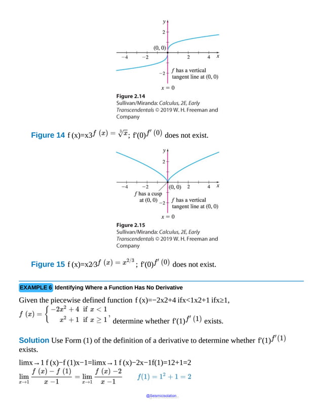
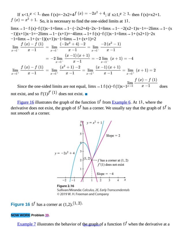
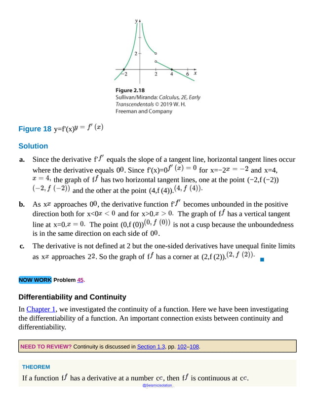
487. Proof To show that f is continuous at c , we need to verify that limx→c f (x)=f (c).
We begin by observing that if x≠c, then
f (x)−f (c)=f (x)−f (c)x−c (x−c)
We take the limit of both sides as x→c, and use the fact that the limit of a product
equals the product of the limits (we show later that each limit exists).
limx→c [f (x)−f (c)]=limx→c f (x)−f (c)x−c(x−c)=limx→c f (x)−f (c)x−climx→c (x−c)
Since f has a derivative at c, we know that
limx→c f (x)−f (c)x−c=f′(c)
is a number. Also for any real number c, limx→c (x−c)=0. So
limx→c [f (x)−f (c)]=[f′(c)]limx→c (x−c)=f′(c)⋅0=0
That is, limx→c f (x)=f (c), so f is continuous at c . ▪
An equivalent statement of this theorem gives a condition under which a function has no
derivative.
COROLLARY
If a function f is discontinuous at a number c , then f has no derivative at c .
IN WORDS Differentiability implies continuity, but continuity does not imply differentiability.
Let’s look at some of the possibilities. In Figure 19(a), the function f is continuous at
the number 1 and has a derivative at 1 . The function g , graphed in Figure 19(b), is
continuous at the number 0 , but it has no derivative at 0 . So continuity at a number c
provides no prediction about differentiability. On the other hand, the function h graphed in
Figure 19(c) illustrates the corollary: If h is discontinuous at a number, it has no derivative
at that number.
@Seismicisolation
@Seismicisolation

488. Figure 19
Diagram
shows
the
functions
f
continuous
at
(1,
1),
g
continuous
at
(0,
0)
and
h
discontinuous
at
(0,
0).
The corollary is useful if we are seeking the derivative of a function f that we suspect is
discontinuous at a number c . If we can show that f is discontinuous at c , then the
corollary affirms that the function f has no derivative at c . For example, since the floor
function f (x)=⌊x⌋ is discontinuous at every integer c , it has no derivative at an
integer.
EXAMPLE 9 Determining Whether a Function Has a Derivative at a Number
Determine whether the function
f (x)=2x+2 if x<35 if x=3x2−1 if x>3
has a derivative at 3 .
Solution Since f is a piecewise-defined function, it may be discontinuous at 3 and
therefore has no derivative at 3 . So we begin by determining whether f is continuous at 3
.
Since f (3)=5, the function f is defined at 3 . Use one-sided limits to check
whether limx→3 f (x) exists.
limx→3− f (x)=limx→3− (2x+2)=8limx→3+ f (x)=limx→3+ (x2−1)=8
Since limx→3− f (x)=limx→3+ f (x), then limx→3 f (x)
exists. But limx→3 f (x)=8 and f (3)=5, so f is discontinuous at 3 .
@Seismicisolation
@Seismicisolation

489. From the corollary, since f is discontinuous at 3 , the function f does not have a
derivative at 3 .
▪
Figure 20 shows the graph of f .
Figure 20 f (x)=2x+2 if x<35 if x=3x2−1 if x>3
NOW WORK Problem 43.
In Example 9, the function f is discontinous at 3 , so by the corollary, the derivative of
f at 3 does not exist. But when a function is continuous at a number c , then sometimes
the derivative at c exists and other times the derivative at c does not exist.
EXAMPLE 10 Determining Whether a Function Has a Derivative at a Number
Determine whether each piecewise-defined function has a derivative at c . If the function has
a derivative at c , find it.
a. f (x)=x3 if x<0x2 if x≥0c=0
b. g(x)=1−2x if x≤1x−2 if x>1c=1
Solution a. See Figure 21. The function f is continuous at 0, which you should verify.
To determine whether f has a derivative at 0, we examine the one-sided limits at 0 using
@Seismicisolation
@Seismicisolation

490. Form (1).
For x<0,
limx→0− f (x)−f (0)x−0=limx→0− x3−0x=limx→0− x2=0
For x>0,
limx→0+ f (x)−f (0)x−0=limx→0+ x2−0x=limx→0+ x=0
Since both one-sided limits are equal, f has a derivative at 0 , and f′(0)=0.
Figure 21 f (x)=x3 if x<0x2 if x≥0
b. See Figure 22. The function g is continuous at 1, which you should verify. To
determine whether g has a derivative at 1, examine the one-sided limits at 1 using Form
(1).
For x<1,
limx→1− g(x)−g(1)x−1=limx→1− (1−2x)−(−1)x−1=limx→1− 2−2xx−1=limx→1− −2(x
−1)x−1=limx→1− (−2)=−2
@Seismicisolation
@Seismicisolation

491. For x>1,
limx→1+ g(x)−g(1)x−1=limx→1+ (x−2)−(−1)x−1=limx→1+ x−1x−1=1
The one-sided limits are not equal, so limx→1 g(x)−g(1)x−1 does not exist.
That is, g has no derivative at 1 . ▪
Figure 22 g(x)=1−2x if x≤1x−2 if x>1
Notice in Figure 21 the tangent lines to the graph of f turn smoothly around the origin.
On the other hand, notice in Figure 22 the tangent lines to the graph of g change abruptly at
the point (1, −1), where the graph of g has a corner.
NOW WORK Problem 41.
2.2 Assess Your Understanding
Concepts and Vocabulary
1. True or False The domain of a function f and the domain of its derivative function f
′ are always equal.
2. True or False If a function is continuous ata number c , then it is differentiable at c .
@Seismicisolation
@Seismicisolation

492. 3. Multiple Choice If f is continuous at a number c and if limx→c f (x)−f (c)x−c
is infinite, then the graph of f has [(a) a horizontal (b) a vertical (c)
no] tangent line at c .
4. The instruction, “Differentiate f ,” means to find the _____ of f .
Skill Building
In Problems 5–10, find the derivative of each function f at any real number c . Use Form (1)
on page 163.
5. f (x)=10
6. f (x)=−4
7. f (x)=2x+3
8. f (x)=3x−5
9. f (x)=2−x2
10. f (x)=2x2+4
In Problems 11–16, differentiate each function f and determine the domain of f′ . Use Form
(3) on page 164.
11. f (x)=5
12. f (x)=−2
13. f (x)=3x2+x+5
14. f (x)=2x2−x−7
15. f (x)=5x−1
16. f (x)=4x+3
In Problems 17–22, differentiate each function f . Graph y=f (x) and y=f′(x)
on the same set of coordinate axes.
17. f (x)=13 x+1
@Seismicisolation
@Seismicisolation

493. 18. f (x)=−4x−5
19. f (x)=2x2−5x
20. f (x)=−3x2+2
21. f (x)=x3−8x
22. f (x)=−x3−8
In Problems 23–26, for each figure determine if the graphs represent a function f and its
derivative f′ . If they do, indicate which is the graph of f and which is the graph of f′ .
23.
24.
@Seismicisolation
@Seismicisolation

494. 25.
26.
In Problems 27–30, use the graph of f to obtain the graph of f′ .
27.
@Seismicisolation
@Seismicisolation

495. 28.
29.
30.
In Problems 31–34, the graph of a function f is given. Match each graph to the graph of its
derivative f′ in A–D.
@Seismicisolation
@Seismicisolation

496. 31.
32.
33.
@Seismicisolation
@Seismicisolation

497. 34.
@Seismicisolation
@Seismicisolation

498. In Problems 35–44, determine whether each function f has a derivative at c. If it does, what is
f′(c)? If it does not, give the reason why.
35. f (x)=x2⁄3 at c=−8
36. f (x)=2x1⁄3 at c=0
37. f (x)=|x2−4| at c=2
38. f (x)=|x2−4| at c=−2
@Seismicisolation
@Seismicisolation

499. 39. f (x)= 2x+3 if x<1x2+4 if x≥1 at c=1
40. f (x)= 3−4x if x<−12x+9 if x≥−1 at c=−1
41. f (x)= −4+2x if x≤124x2−4 if x>12 at c=12
42. f (x)= 2x2+1 if x<−1−1−4x if x≥−1 at c=−1
43. f (x)=2x2+1 if x<−12+2x if x≥−1at c=−1
44. f (x)= 5−2x if x<2x2 if x≥2 at c=2
In Problems 45–48, each function f is continuous for all real numbers, and the graph of y=f
′(x) is given.
a. Does the graph of f have any horizontal tangent lines? If yes, explain why and identify
where they occur.
b. Does the graph of f have any vertical tangent lines? If yes, explain why, identify where
they occur, and determine whether the point is a cusp of f.
c. Does the graph of f have any corners? If yes, explain why and identify where they occur.
@Seismicisolation
@Seismicisolation

500. 45.
46.
47.
@Seismicisolation
@Seismicisolation

501. 48.
In Problems 49 and 50, use the given points (c,f (c)) on the graph of the function f .
a. For which numbers c does limx→c f (x) exist but f is not continuous at c ?
b. For which numbers c is f continuous at c but not differentiable at c ?
49.
50.
In Problems 51–54, find the derivative of each function.
@Seismicisolation
@Seismicisolation

502. 51. f (x)=mx+b
52. f (x)=ax2+bx+c
53. f (x)=1x2
54. f (x)=1x
Applications and Extensions
In Problems 55–66, each limit represents the derivative of a function f at some number c .
Determine f and c in each case.
55. limh→0 (2+h)2−4h
56. limh→0 (2+h)3−8h
57. limx→1 x2−1x−1
58. limx→1 x4−1x−1
59. limh→0 9+h−3h
60. limh→0 (8+h)1⁄3−2h
61. limx→π⁄6 sin x−12x−π6
62. limx→π⁄4 cos x−22x−π4
63. limx→0 2(x+2)2−(x+2)−6x
@Seismicisolation
@Seismicisolation

503. 64. limx→0 3x3−2xx
65. limh→0 (3+h)2+2(3+h)−15h
66. limh→0 3(h−1)2+h−3h
67. Units The volume V (in cubic feet) of a balloon is expanding according to
V=V(t)=4t, where t is the time (in seconds). At what rate is the volume
changing with respect to time? What are the units of V′(t) ?
68. Units The area A (in square miles) of a circular patch of oil is expanding according to
A=A(t)=2t, where t is the time (in hours). At what rate is the area
changing with respect to time? What are the units of A′(t) ?
69. Units A manufacturer of precision digital switches has a daily cost C (in dollars) of
C(x)=10,000+3x, where x is the number of switches produced
daily. What is the rate of change of cost with respect to x ? What are the units of C′(x)
?
70. Units A manufacturer of precision digital switches has daily revenue R (in dollars) of
R(x)=5x−x22000, where x is the number of switches produced
daily. What is the rate of change of revenue with respect to x ? What are the units of R
′(x) ?
71. f (x)=x3 if x≤0x2 if x>0
a. Determine whether f is continuous at 0 .
b. Determine whether f′(0) exists.
c. Graph the function f and its derivative f′.
72. For the function f (x)=2x if x≤0x2 if x>0
a. Determine whether f is continuous at 0 .
b. Determine whether f′(0) exists.
c. Graph the function f and its derivative f′.
73. Velocity The distance s (in feet) of an automobile from the origin at time t (in
@Seismicisolation
@Seismicisolation

504. seconds) is given by the position function
s=s(t)=t3 if 0≤t<5125 if t≥5
(This could represent a crash test in which a vehicle is accelerated until it hits a brick wall at t=5 s. )
a. Find the velocity just before impact (at t=4.99 s) and just after impact (at
t=5.01 s).
b. Is the velocity function v=s′(t) continuous at t=5?
c. How do you interpret the answer to (b)?
74. Population Growth A simple model for population growth states that the rate of change
of population size P with respect to time t is proportional to the population size.
Express this statement as an equation involving a derivative.
75. Atmospheric Pressure Atmospheric pressure p decreases as the distance x from the
surface of Earth increases, and the rate of change of pressure with respect to altitude is
proportional to the pressure. Express this law as an equation involving a derivative.
76. Electrical Current Under certain conditions, an electric current I will die out at a rate
(with respect to time t ) that is proportional to the current remaining. Express this law
as an equation involving a derivative.
77. Tangent Line Let f (x)=x2+2. Find all points on the graph of f for
which the tangent line passes through the origin.
78. Tangent Line Let f (x)=x2−2x+1. Find all points on the graph of f
for which the tangent line passes through the point (1,−1).
79. Area and Circumference of a Circle A circle of radius r has area A=πr2 and
circumference C=2πr. If the radius changes from r to r+Δr, find the:
a. Change in area.
b. Change in circumference.
c. Average rate of change of area with respect to radius.
d. Average rate of change of circumference with respect to radius.
e. Rate of change of circumference with respect to radius.
80. Volume of a Sphere The volume V of a sphere of radius r is V=4πr33.
If the radius changes from r to r+Δr, find the:
a. Change in volume.
b. Average rate of change of volume with respect to radius.
@Seismicisolation
@Seismicisolation

505. c. Rate of change of volume with respect to radius.
81. Use the definition of the derivative to show that f (x)=x has no derivative at
0 .
82. Use the definition of the derivative to show that f (x)=x3 has no derivative at
0 .
83. If f is an even function that is differentiable at c , show that its derivative function is
odd. That is, show f′(−c)=−f′(c).
84. If f is an odd function that is differentiable at c , show that its derivative function is
even. That is, show f′(−c)=f′(c).
85. Tangent Lines and Derivatives Let f and g be two functions, each with derivatives
at c . State the relationship between their tangent lines at c if:
a. f′(c)=g′(c)
b. f′(c)=−1g′(c)g′(c)≠0
Challenge Problems
86. Let f be a function defined for all real numbers x . Suppose f has the following
properties:
f (u+v)=f (u)f (v)f (0)=1f′(0) exists
a. Show that f′(x) exists for all real numbers x .
b. Show that f′(x)=f′(0)f (x).
87. A function f is defined for all real numbers and has the following three properties:
f (1)=5f (3)=21f (a+b)−f (a)=kab+2b2
for all real numbers a and b where k is a fixed real number independent of a and b .
a. Use a=1 and b=2 to find k .
b. Find f′(3).
c. Find f′(x) for all real x .
88. A function f is periodic if there is a positive number p so that f (x+p)=f (x)
for all x . Suppose f is differentiable. Show that if f is periodic
with period p , then f′ is also periodic with period p .
@Seismicisolation
@Seismicisolation

506. 1. = NOW WORK problem
= Graphing technology recommended
= Computer Algebra System recommended
* The one-sided limits, limx→c− f (x)−(c)x−c and limx→c+ f (x)−(c)x−c are
called the left-hand derivative of f at c , denoted f−′(c), and the right-hand derivative of f at c , denoted
f+′(c), respectively. Using properties of limits, the derivative f′(c) exists if and only if f−′(c)=f+′(c).
@Seismicisolation
@Seismicisolation

507. 2.3 The Derivative of a Polynomial Function; The
Derivative of y=ex
OBJECTIVES When you finish this section, you should be able to:
1 Differentiate a constant function
2 Differentiate a power function
3 Differentiate the sum and the difference of two functions
4 Differentiate the exponential function y = ex
Finding the derivative of a function from the definition can become tedious, especially if the
function f is complicated. Just as we did for limits, we derive some basic derivative
formulas and some properties of derivatives that make finding a derivative simpler.
Before getting started, we introduce other notations commonly used for the derivative f
′(x) of a function y=f (x). The most common ones are
y′dydxDf (x)
Leibniz notation dydx may be written in several equivalent ways as
dydx=ddx y=ddx f (x)
where ddx is an instruction to find the derivative (with respect to the independent
variable x ) of the function y=f (x).
In operator notation Df (x), D is said to operate on the function, and the
result is the derivative of f. To emphasize that the operation is performed with respect to
the independent variable x, it is sometimes written Df (x)=Dxf (x).
We use prime notation or Leibniz notation, or sometimes a mixture of the two, depending
on which is more convenient. We do not use the notation Df (x) in this book.
1 Differentiate a Constant Function
See Figure 23. Since the graph of a constant function f (x)=A is a horizontal line,
the tangent line to f at any point is also a horizontal line, whose slope is 0. Since the
derivative is the slope of the tangent line, the derivative of f is 0.
@Seismicisolation
@Seismicisolation

508. Figure 23 f(x)=A
THEOREM Derivative of a Constant Function
If f is the constant function f(x)=A, then
f′(x)=0
That is, if A is a constant, then
ddx A=0
IN WORDS The derivative of a constant is 0.
Proof If f(x)=A, then its derivative function is given by
▪
EXAMPLE 1 Differentiating a Constant Function
a. If f(x)=3, then f′(x)=0
b. If f(x)=−12, then f′(x)=0
@Seismicisolation
@Seismicisolation

509. c. If f(x)=π, then ddxπ=0
d. If f(x)=0, then ddx 0=0
▪
2 Differentiate a Power Function
Next we analyze the derivative of a power function f(x)=xn, where n≥1 is
an integer.
When n=1, then f(x)=x is the identity function and its graph is the line
y=x, as shown in Figure 24.
Figure 24 f(x)=x
The slope of the line y=x is 1, so we would expect f′(x)=1.
Proof
▪
THEOREM Derivative of f(x)=x
If f(x)=x, then
@Seismicisolation
@Seismicisolation

510. f′(x)=ddx x=1
When n=2, then f(x)=x2 is the square function. The derivative of f is
f
′(x)=ddx x2=limh→0 (x+h)2−x2h=limh→0 x2+2hx+h2−x2h=limh→0 h(2x+h)h=limh→0(2x+
The slope of the tangent line to the graph of f(x)=x2 is different for every
number x. Figure 25 shows the graph of f and several of its tangent lines. Notice that the
slope of each tangent line drawn is twice the value of x.
Figure 25 f(x)=x2
It
is
the
graph
of
the
function
x-
square.
The
When n=3, then f(x)=x3 is the cube function. The derivative of f is
f
′(x)=limh→0 (x+h)3−x3h=limh→0 x3+3x2h+3xh2+h3−x3h=limh→0 h(3x2+3xh+h2)h=limh→
Notice that the derivative of each of these power functions is another power function,
whose degree is 1 less than the degree of the original function and whose coefficient is the
degree of the original function. This rule holds for all power functions as the following
@Seismicisolation
@Seismicisolation

511. theorem, called the Simple Power Rule, indicates.
THEOREM Simple Power Rule
The derivative of the power function y=xn, where n≥1 is an integer, is
y′=ddx xn=nxn−1
IN WORDS The derivative of x raised to an integer power n≥1 is n times x raised to the power n
−1.
Proof If f(x)=xn and n is a positive integer, then f(x+h)=(x+h)n.
We use the Binomial Theorem to expand (x+h)n. Then
f(x+h)=(x+h)n=xn+nxn−1h+n(n−1)2 xn−2h2+n(n−1)(n−2)6 xn−3h3+⋯+nxhn−1+hn
f ′(x)=limh→0 f(x+h)−f(x)h =limh→0 xn+nxn−1h+nn−12 xn−2h2+n(n−1)(n−2)6 xn−3h3+⋯
+nxhn−1+hn−xnh =limh→0 nxn−1h+n(n−1)2 xn−2h2+n(n−1)(n−2)6 xn−3h3+⋯+nxhn
−1+hnh Simplify.=limh→0 hnxn−1+n(n−1)2 xn−2h+n(n−1)(n−2)6 xn−3h2+⋯+nxhn−2+hn
−1h Factor h in the numerator.=limh→0 nxn−1+n(n−1)2 xn−2h+n(n−1)(n−2)6 xn−3h2+⋯
+nxhn−2+hn−1Divide out the common h.=nxn−1 Take the limit. Only the firstterm remains.▪
NEED TO REVIEW? The Binomial Theorem is discussed in Section P.8, pp. 73–74.
EXAMPLE 2 Differentiating a Power Function
@Seismicisolation
@Seismicisolation

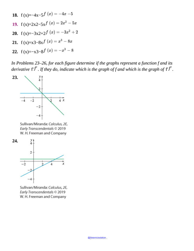
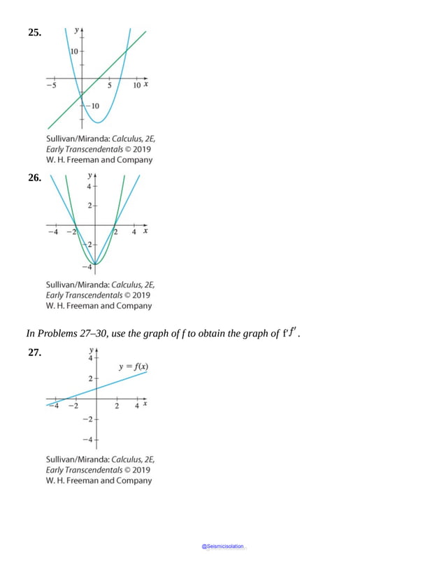
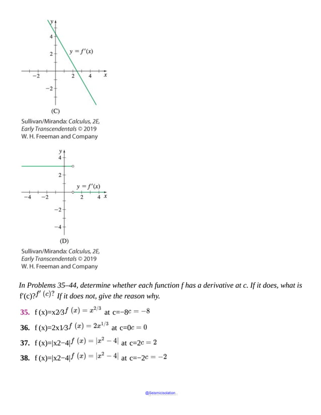
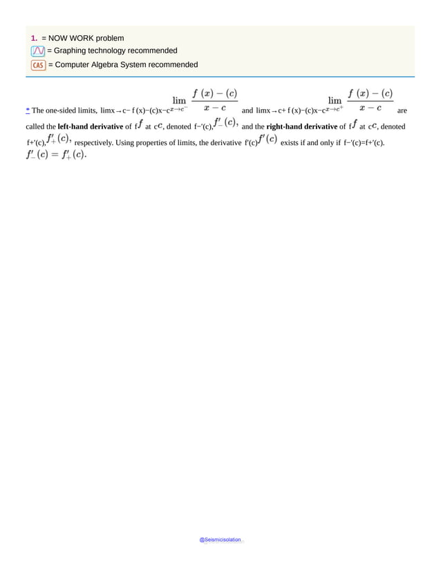
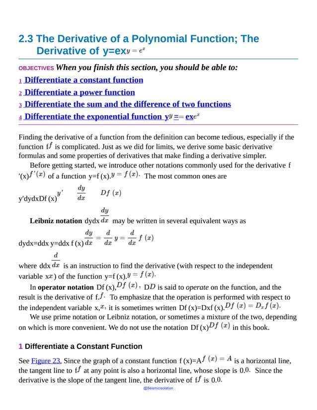
512. a. ddx x5=5x4
b. If g(x)=x10, then g′(x)=10x9.
▪
NOW WORK Problem 1.
Note: ddx xn=nxn−1 is true not only for positive integers n but also for any
real number n. But the proof requires future results. As these are developed, we will
expand the Power Rule to include an ever-widening set of numbers until we arrive at the fact
it is true when n is a real number.
But what if we want to find the derivative of the function f(x)=axn when a≠1
? The next theorem, called the Constant Multiple Rule, provides a way.
THEOREM Constant Multiple Rule
If a function f is differentiable and k is a constant, then F(x)=kf(x) is a
function that is differentiable and
F′(x)=kf′(x)
IN WORDS The derivative of a constant times a dierentiable function f equals the constant times the
derivative of f.
Proof Use the definition of a derivative, Form (3).
F′(x)=limh→0 F(x+h)−F(x)h=limh→0 kf(x+h)−kf(x)h=limh→0 kf(x+h)
−f(x)h=k⋅limh→0 f(x+h)−f(x)h=k⋅f′(x)
▪
Using Leibniz notation, the Constant Multiple Rule takes the form
ddx[kf(x)]=kddx f(x)
@Seismicisolation
@Seismicisolation

513. A change in the symbol used for the independent variable does not affect the derivative
formula. For example, ddt t2=2t and ddu u5=5u4.
EXAMPLE 3 Differentiating a Constant Times a Power Function
Find the derivative of each function:
a. f(x)=5x3
b. g(u)=−12 u2
c. u(x)=π4x3
Solution Notice that each of these functions involves the product of a constant and a power
function. So, we use the Constant Multiple Rule followed by the Simple Power Rule.
a. f(x)=5⋅x3, so f′(x)=5ddx x3=5⋅3x2=15x2
b. g(u)=−12⋅u2, so g′(u)=−12⋅ddu u2=−12⋅2u1=−u
▪
NOW WORK Problem 31.
3 Differentiate the Sum and the Difference of Two Functions
We can find the derivative of a function that is the sum of two functions whose derivatives
are known by adding the derivatives of each function.
THEOREM Sum Rule
If two functions f and g are differentiable and if F(x)=f(x)+g(x),
then F is differentiable and
@Seismicisolation
@Seismicisolation

514. F′(x)=f′(x)+g′(x)
IN WORDS The derivative of the sum of two differentiable functions equals the sum of their derivatives. That is,
(f+g)′=f′+g′.
Proof If F(x)=f(x)+g(x), then
F(x+h)−F(x)=[f(x+h)+g(x+h)]−[f(x)+g(x)]=[f(x+h)−f(x)]+[g(x+h)−g(x)]
So, the derivative of F is
F′(x)=limh→0 [f(x+h)−f(x)]+[g(x+h)−g(x)]h=limh→0 f(x+h)−f(x)h+limh→0 g(x+h)
−g(x)hThe limit of a sum is the sum of the limits.=f′(x)+g′(x)
▪
In Leibniz notation, the Sum Rule takes the form
ddx[f(x)+g(x)]=ddx f(x)+ddx g(x)
EXAMPLE 4 Differentiating the Sum of Two Functions
Find the derivative of f(x)=3x2+8.
Solution Here f is the sum of 3x2 and 8. So, we begin by using the Sum Rule.
▪
NOW WORK Problem 7.
@Seismicisolation
@Seismicisolation

515. THEOREM Difference Rule
If the functions f and g are differentiable and if F(x)=f(x)−g(x),
then F is differentiable, and F′(x)=f′(x)−g′(x). That is,
ddx[f(x)−g(x)]=ddx f(x)−ddx g(x)
IN WORDS The derivative of the difference of two differentiable functions is the difference of their derivatives.
That is, (f−g)′=f′−g′.
The proof of the Difference Rule is left as an exercise. (See Problem 78.)
The Sum and Difference Rules extend to sums (or differences) of more than two
functions. That is, if the functions f1,f2,…,fn are all differentiable, and a1,a2,
…,an are constants, then
ddx[a1 f1(x) +a2 f2(x) + ⋯ + an fn(x)]=a1 ddxf1(x)+a2 ddxf2(x)+⋯+an ddxfn(x)
Combining the rules for finding the derivative of a constant, a power function, and a sum
or difference allows us to differentiate any polynomial function.
EXAMPLE 5 Differentiating a Polynomial Function
a. Find the derivative of f(x)=2x4−6x2+2x−3.
b. What is f′(2)?
c. Find the slope of the tangent line to the graph of f at the point (1,−5).
d. Find an equation of the tangent line to the graph of f at the point (1,−5).
e. Find an equation of the normal line to the graph of f at the point (1,−5).
f. Use technology to graph f, the tangent line, and the normal line to the graph of f at
the point (1,−5) on the same screen.
Solution a.
@Seismicisolation
@Seismicisolation

516. b. f′(2)=8⋅23−12⋅2+2=64−24+2=42.
c. The slope of the tangent line at the point (1,−5) equals f′(1).
f′(1)=8⋅13−12⋅1+2=8−12+2=−2
d. Use the point-slope form of an equation of a line to find an equation of the tangent line at
(1,−5).
y−(−5)=−2(x−1)y=−2(x−1)−5=−2x+2−5=−2x−3
The line y=−2x−3 is tangent to the graph of f(x)=2x4−6x2+2x−3
at the point (1,−5).
e. Since the normal line and the tangent line at the point (1,−5) on the graph of f are
perpendicular and the slope of the tangent line is −2, the slope of the normal line is 12.
Use the point-slope form of an equation of a line to find an equation of the normal line.
y−(−5)=12 (x−1)y=12 (x−1)−5=12 x−12−5=12 x−112
The line y=12x−112 is normal to the graph of f at the point (1,−5).
f. The graphs of f, the tangent line, and the normal line to f at 1,−5 are shown in
Figure 26.
▪
@Seismicisolation
@Seismicisolation

517. Figure 26 f(x)=2x4−6x2+2x−3
NOW WORK Problem 33.
In some applications, we need to solve equations or inequalities involving the derivative
of a function.
EXAMPLE 6 Solving Equations and Inequalities Involving Derivatives
a. Find the points on the graph of f(x)=4x3−12x2+2, where f has
a horizontal tangent line.
b. Where is f′(x)>0 ? Where is f′(x)<0 ?
Solution a. The slope of a horizontal tangent line is 0. Since the derivative of f equals
the slope of the tangent line, we need to find the numbers x for which f′(x)=0.
f′(x)=12x2−24x=12x (x−2) 12x (x−2)=0 f′(x)=0x=0 or x=2Solve.
At the points (0,f(0))=(0,2) and (2,f(2))=(2,−14),
the graph of the function f(x)=4x3−12x2+2 has horizontal tangent
lines.
b. Since f′(x)=12x(x−2) and we want to solve the inequalities f′(x)>0
and f′(x)<0, we use the zeros of f′, 0 and 2, and form a table using
@Seismicisolation
@Seismicisolation

518. the intervals (−∞,0 ), (0,2 ), and (2,∞ ).
▪
TABLE 2
Interval (−∞,0) (0,2) (2,∞)
Sign of f′(x)=12x(x−2) Positive Negative Positive
We conclude f′(x)>0 on (−∞,0)∪(2,∞) and f′(x)<0
on (0,2).
Figure 27 shows the graph of f and the two horizontal tangent lines.
▪
Figure 27 f(x)=4x3−12x2+2
NOW WORK Problem 37.
4 Differentiate the Exponential Function y=ex
None of the differentiation rules developed so far allows us to find the derivative of an
exponential function. To differentiate f(x)=ax, we return to the definition of a
derivative.
NEED TO REVIEW? Exponential functions are discussed in Section P.5, pp. 41–44.
We begin by making some general observations about the derivative of f(x)=ax,
@Seismicisolation
@Seismicisolation

519. a>0 and a≠1. We then use these observations to find the derivative of
the exponential function y=ex.
Suppose f(x)=ax, where a>0 and a≠1. The derivative of f is
provided limh→0 ah−1h exists.
Three observations about the derivative are significant:
f′(0)=a0limh→0 ah−1h=limh→0 ah−1h.
f′(x) is a multiple of ax. In fact, ddx ax=f′(0)⋅ax.
If f′(0) exists, then f′(x) exists, and the domain of f′ is the same as that of
f(x)=ax, all real numbers.
The slope of the tangent line to the graph of f(x)=ax at the point (0,1) is f
′(0)=limh→0 ah−1h, and the value of this limit depends on the base a.
In Section P.5, the number e was defined as that number for which the slope of the tangent
line to the graph of y=ax at the point (0,1) equals 1. That is, if f(x)=ex,
then f′(0)=1 so that
limh→0 eh−1h=1
Figure 28 shows f(x)=ex and the tangent line y=x+1 with slope 1 at the
point (0,1).
@Seismicisolation
@Seismicisolation

520. (1)
Figure 28
NEED TO REVIEW? The number e is discussed in Section P.5, pp. 44–45.
Since ddx ax=f′(0)⋅ax, if f(x)=ex, then ddx ex=f
′(0)⋅ex=1⋅ex=ex.
THEOREM Derivative of the Exponential Function y=ex
The derivative of the exponential function y=ex is
y′=ddx ex=ex
EXAMPLE 7 Differentiating an Expression Involving y=ex
Find the derivative of f(x)=4ex+x3.
Solution The function f is the sum of 4ex and x3. Then
▪
@Seismicisolation
@Seismicisolation

521. NOW WORK Problem 25.
Now we know ddx ex=ex. To find the derivative of f(x)=ax, a>0
and a≠1, we need more information. See Chapter 3.
2.3 Assess Your Understanding
Concepts and Vocabulary
1. ddx π2=______ ; ddx x3=______.
2. When n is a positive integer, the Simple Power Rule states that ddx xn=______.
3. True or False The derivative of a power function of degree greater than 1 is also a
power function.
4. If k is a constant and f is a differentiable function, then ddx[kf(x)]=______.
5. The derivative of f(x)=ex is _____.
6. True or False The derivative of an exponential function f(x)=ax, where
a>0 and a≠1, is always a constant multiple of ax.
Skill Building
In Problems 7–26, find the derivative of each function using the formulas of this section. (a,
b, c, and d, when they appear, are constants.)
7. f(x)=3x+2
8. f(x)=5x−π
9. f(x)=x2+3x+4
10. f(x)=4x4+2x2−2
11. f(u)=8u5−5u+1
@Seismicisolation
@Seismicisolation

522. 12. f(u)=9u3−2u2+4u+4
13. f(s)=as3+32 s2
14. f(s)=4−πs2
15. f(t)=13 (t5−8)
16. f(x)=15 (x7−3x2+2)
17. f(t)=t3+25
18. f(x)=x7−5x9
19. f(x)=x3+2x+17
20. f(x)=1a (ax2+bx+c),a≠0
21. f(x)=ax2+bx+c
22. f(x)=ax3+bx2+cx+d
23. f(x)=4ex
24. f(x)=−12 ex
25. f(u)=5u2−2eu
26. f(u)=3eu+10
In Problems 27–32, find each derivative.
27. ddt 3 t+12
28. ddt 2t4−58
29. dAdR if A(R)=πR2
@Seismicisolation
@Seismicisolation

523. 30. dCdR if C=2πR
31. dVdr if V=43πr3
32. dPdT if P=0.2T
In Problems 33–36:
a. Find the slope of the tangent line to the graph of each function f at the indicated point.
b. Find an equation of the tangent line at the point.
c. Find an equation of the normal line at the point.
d. Graph f and the tangent line and normal line found in (b) and (c) on the same set of axes.
33. f(x)=x3+3x−1 at (0,−1)
34. f(x)=x4+2x−1 at (1,2)
35. f(x)=ex+5x at (0,1)
36. f(x)=4−ex at (0,3)
In Problems 37–42:
a. Find the points, if any, at which the graph of each function f has a horizontal tangent
line.
b. Find an equation for each horizontal tangent line.
c. Solve the inequality f′(x)>0.
d. Solve the inequality f′(x)<0.
e. Graph f and any horizontal lines found in (b) on the same set of axes.
f. Describe the graph of f for the results obtained in parts (c) and (d).
37. f(x)=3x2−12x+4
38. f(x)=x2+4x−3
39. f(x)=x+ex
40. f(x)=2ex−1
@Seismicisolation
@Seismicisolation

524. 41. f(x)=x3−3x+2
42. f(x)=x4−4x3
43. Rectilinear Motion At t seconds, an object in rectilinear motion is s meters from the
origin, where s(t)=t3−t+1. Find the velocity of the object at t=0
and at t=5.
44. Rectilinear Motion At t seconds, an object in rectilinear motion is s meters from the
origin, where s(t)=t4−t3+1. Find the velocity of the object at t=0
and at t=1.
Rectilinear Motion In Problems 45 and 46, each position function gives the signed distance
s from the origin at time t of an object in rectilinear motion:
a. Find the velocity v of the object at any time t .
b. When is the object at rest?
45. s(t)=2−5t+t2
46. s(t)=t3−92 t2+6t+4
In Problems 47 and 48, use the graphs to find each derivative.
47. Let u(x)=f(x)+g(x) and v(x)=f(x)−g(x).
a. u′(0)
b. u′(4)
c. v′(−2)
d. v′(6)
e. 3u′(5)
f. −2v′(3)
@Seismicisolation
@Seismicisolation

525. 48. Let F(t)=f(t)+g(t) and G(t)=g(t)−f(t).
a. F′(0)
b. F′(3)
c. F′(−4)
d. G′(−2)
e. G′(−1)
f. G′(6)
In Problems 49 and 50, for each function f :
a. Find f′(x) by expanding f(x) and differentiating the polynomial.
@Seismicisolation
@Seismicisolation

526. b. Find f′(x) using a CAS.
c. Show that the results found in parts (a) and (b) are equivalent.
49. f(x)=(2x−1)3
50. f(x)=(x2+x)4
Applications and Extensions
In Problems 51–56, find each limit.
51. limh→0 512+h8−5128h
52. limh→0 6(2+h)5−6⋅25h
53. limh→0 3(8+h)5−3⋅85h
54. limh→0 π(1+h)10−πh
55. limh→0 a(x+h)3−ax3h
56. limh→0 b(x+h)n−bxnh
In Problems 57–62, find an equation of the tangent line(s) to the graph of the function f that
is (are) parallel to the line L.
57. f(x)=3x2−x ; L : y=5x
58. f(x)=2x3+1 ; L : y=6x−1
59. f(x)=ex ; L : y−x−5=0
60. f(x)=−2ex ; L : y+2x−8=0
61. f(x)=13 x3−x2 ; L : y=3x−2
62. f(x)=x3−x ; L : x+y=0
@Seismicisolation
@Seismicisolation

527. 63. Tangent Lines Let f(x)=4x3−3x−1.
a. Find an equation of the tangent line to the graph of f at x=2.
b. Find the coordinates of any points on the graph of f where the tangent line is parallel to y=x+12.
c. Find an equation of the tangent line to the graph of f at any points found in (b).
d. Graph f, the tangent line found in (a), the line y=x+12, and any tangent
lines found in (c) on the same screen.
64. Tangent Lines Let f(x)=x3+2x2+x−1.
a. Find an equation of the tangent line to the graph of f at x=0.
b. Find the coordinates of any points on the graph of f where the tangent line is parallel to y=3x−2.
c. Find an equation of the tangent line to the graph of f at any points found in (b).
d. Graph f, the tangent line found in (a), the line y=3x−2, and any tangent
lines found in (c) on the same screen.
65. Tangent Line Show that the line perpendicular to the x -axis and containing the point
(x,y) on the graph of y=ex and the tangent line to the graph of y=ex
at the point (x,y) intersect the x -axis 1 unit apart. See the figure.
66. Tangent Line Show that the tangent line to the graph of y=xn, n≥2 an
integer, at (1,1) has y -intercept 1−n.
67. Tangent Lines If n is an odd positive integer, show that the tangent lines to the graph
of y=xn at (1,1) and at (−1,−1) are parallel.
68. Tangent Line If the line 3x−4y=0 is tangent to the graph of y=x3+k
in the first quadrant, find k.
@Seismicisolation
@Seismicisolation

528. 69. Tangent Line Find the constants a,b, and c so that the graph of y=ax2+bx+c
contains the point (−1,1) and is tangent to the line y=2x
at (0,0).
70. Tangent Line Let T be the tangent line to the graph of y=x3 at the point 12,18.
At what other point Q on the graph of y=x3 does the line T
intersect the graph? What is the slope of the tangent line at Q ?
71. Military Tactics A dive bomber is flying from right to left along the graph of y=x2.
When a rocket bomb is released, it follows a path that is approximately along
the tangent line. Where should the pilot release the bomb if the target is at (1,0) ?
72. Military Tactics Answer the question in Problem 71 if the plane is flying from right to
left along the graph of y=x3.
73. Fluid Dynamics The velocity v of a liquid flowing through a cylindrical tube is given
by the Hagen‑Poiseuille equation v=k(R2−r2), where R is the
radius of the tube, k is a constant that depends on the length of the tube and the
velocity of the liquid at its ends, and r is the variable distance of the liquid from the
center of the tube. See the figure below.
a. Find the rate of change of v with respect to r at the center of the tube.
b. What is the rate of change halfway from the center to the wall of the tube?
c. What is the rate of change at the wall of the tube?
74. Rate of Change Water is leaking out of a swimming pool that measures 20 ft by 40 ft
by 6 ft. The amount of water in the pool at a time t is W(t)=35,000−20t2
gallons, where t equals the number of hours since the pool was
last filled. At what rate is the water leaking when t=2 h?
75. Luminosity of the Sun The luminosity L of a star is the rate at which it radiates
energy. This rate depends on the temperature T and surface area A of the star’s
photosphere (the gaseous surface that emits the light). Luminosity is modeled by the
equation L=σAT4, where σ is a constant known as the Stefan–Boltzmann
@Seismicisolation
@Seismicisolation

529. constant, and T is expressed in the absolute (Kelvin) scale for which 0 K is absolute
zero. As with most stars, the Sun’s temperature has gradually increased over the 6
billion years of its existence, causing its luminosity to slowly increase.
a. Find the rate at which the Sun’s luminosity changes with respect to the temperature
of its photosphere. Assume that the surface area A remains constant.
b. Find the rate of change at the present time. The temperature of the photosphere is
presently 5800 K (10,000 ∘F), the radius of the photosphere is
r=6.96×108 m, and σ=5.67×10−8Wm2 K4.
c. Assuming that the rate found in (b) remains constant, how much would the
luminosity change if its photosphere temperature increased by 1 K (1 ∘ C or 1.8
∘ F)? Compare this change to the present luminosity of the
Sun.
76. Medicine: Poiseuille’s Equation The French physician Poiseuille discovered that the
volume V of blood (in cubic centimeters per unit time) flowing through an artery with
inner radius R (in centimeters) can be modeled by
V(R)=kR4
where k=π8νl is constant (here ν represents the viscosity of blood and l is the
length of the artery).
a. Find the rate of change of the volume V of blood flowing through the artery with
respect to the radius R.
b. Find the rate of change when R=0.03 and when R=0.04.
c. If the radius of a partially clogged artery is increased from 0.03 to 0.04 cm,
estimate the effect on the rate of change of the volume V with
respect to R of the blood flowing through the enlarged artery.
d. How do you interpret the results found in (b) and (c)?
77. Derivative of an Area Let f(x)=mx, m>0. Let F(x), x>0,
be defined as the area of the shaded region in the figure. Find F′(x).
@Seismicisolation
@Seismicisolation

530. 78. The Difference Rule Prove that if f and g are differentiable functions and if
F(x)=f(x)−g(x), then
F′(x)=f′(x)−g′(x)
79. Simple Power Rule Let f (x)=xn, where n is a positive integer. Use a
factoring principle to show that
f′(c)=limx→c f (x)−f (c)x−c=ncn−1
80. Normal Lines For what nonnegative number b is the line given by y=−13 x+b
normal to the graph of y=x3 ?
81. Normal Lines Let N be the normal line to the graph of y=x2 at the point
(−2,4). At what other point Q does N meet the graph?
Challenge Problems
82. Tangent Line Find a,b,c,d so that the tangent line to the graph of the cubic
y=ax3+bx2+cx+d at the point (1,0) is y=3x−3
and at the point (2,9) is y=18x−27.
83. Tangent Line Find the fourth degree polynomial that contains the origin and to which
the line x+2y=14 is tangent at both x=4 and x=−2.
84. Tangent Lines Find equations for all the lines containing the point 1,4 that are
tangent to the graph of y=x3−10x2+6x−2. At what points do
each of the tangent lines touch the graph?
85. The line x=c, where c>0, intersects the cubic y=2x3+3x2−9
at the point P and intersects the parabola y=4x2+4x+5
at the point Q, as shown in the figure on the right.
a. If the line tangent to the cubic at the point P is parallel to the line tangent to the
@Seismicisolation
@Seismicisolation

531. parabola at the point Q, find the number c.
b. Write an equation for each of the two tangent lines described in (a).
86. f(x)=Ax2+B, A>0.
a. Find c, c>0, in terms of A so that the tangent lines to the graph of f at
(c,f(c)) and (−c,f(−c)) are perpendicular.
b. Find the slopes of the tangent lines in (a).
c. Find the coordinates, in terms of A and B, of the point of intersection of the
tangent lines in (a).
@Seismicisolation
@Seismicisolation

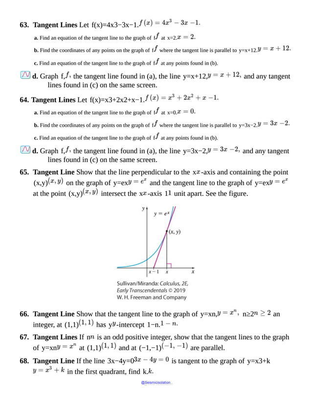
532. 2.4 Differentiating the Product and the Quotient of Two
Functions; Higher-Order Derivatives
OBJECTIVES When you finish this section, you should be able to:
1 Differentiate the product of two functions
2 Differentiate the quotient of two functions
3 Find higher-order derivatives
4 Work with acceleration
In this section, we obtain formulas for differentiating products and quotients of functions. As
it turns out, the formulas are not what we might expect. The derivative of the product of two
functions is not the product of their derivatives, and the derivative of the quotient of two
functions is not the quotient of their derivatives.
1 Differentiate the Product of Two Functions
Consider the two functions f (x)=2x and g(x)=x3. Both are
differentiable, and their derivatives are f′(x)=2 and g′(x)=3x2. Form
the product
f (x)=f (x)g(x)=2x⋅x3=2x4
Now find F′ using the Constant Multiple Rule and the Simple Power Rule.
F′(x)=2⋅4x3=8x3
Notice that f′(x)g′(x)=2⋅3x2=6x2 is not equal to F
′(x)=ddx[f (x)g(x)]=8x3. We conclude that the derivative of a
product of two functions is not the product of their derivatives.
To find the derivative of the product of two differentiable functions f and g, we let
f (x)=f (x)g(x) and use the definition of a derivative, namely,
F′(x)=limh→0 [f (x+h)g(x+h)]−[f (x)g(x)]h
We can express F′ in an equivalent form that contains the difference quotients for f and
g, by subtracting and adding f (x+h)g(x) to the numerator.
F′(x)=limh→0 f (x+h)g(x+h)−f (x+h)g(x)+f (x+h)g(x)−f (x)g(x)h =limh→0 f (x+h)[g(x+h)
@Seismicisolation
@Seismicisolation

533. −g(x)]+[f (x+h)−f (x)]g(x)h Group and factor.=limh→0 f (x+h) limh→0 g(x+h)−g(x)h+
limh→0 f (x+h)−f (x)h limh→0 g(x) Use properties of limits.=limh→0 f (x+h)g′(x)+f
′(x)limh→0 g(x) Definition of a derivative.=f (x)g′(x)+f′(x)g(x) limh→0 g(x)=g(x) since h is
not present. Since f is differentiable, it is continuous, so limh→0 f (x+h)=f (x).
We have proved the following theorem.
THEOREM Product Rule
If f and g are differentiable functions and if f (x)=f (x)g(x), then F
is differentiable, and the derivative of the product F is
F′(x)=[f (x)g(x)]′=f (x)g′(x)+f′(x)g(x)
In Leibniz notation, the Product Rule takes the form
ddx F (x)=ddx[f (x)g(x)]=f (x)ddx g(x)+ ddx f (x) g(x)
IN WORDS The derivative of the product of two differentiable functions equals the first function times the
derivative of the second function plus the derivative of the first function times the second function. That is, (fg)
′=f (g′)+(f′)g.
EXAMPLE 1 Differentiating the Product of Two Functions
Find y′ if y=(1+x2)ex.
Solution The function y is the product of two functions: a polynomial, f (x)=1+x2,
and the exponential function, g(x)=ex. By the Product Rule,
@Seismicisolation
@Seismicisolation

534. At this point, we have found the derivative, but it is customary to simplify the answer.
Then
▪
NOW WORK Problem 9.
Do not use the Product Rule unnecessarily! When one of the factors is a constant, use the
Constant Multiple Rule. For example, it is easier to work
ddx[5(x2+1)]=5 ddx(x2+1)=5⋅2x=10x
than it is to work
ddx[5(x2+1)]=5 ddx(x2+1)+ddx 5 (x2+1)=5⋅2x+0⋅(x2+1)=10x
Also, it is easier to simplify f (x)=x2(4x−3) before finding the derivative.
That is, it is easier to work
ddx[x2(4x−3)]=ddx(4x3−3x2)=12x2−6x
than it is to use the Product Rule
ddx[x2(4x−3)]=x2ddx(4x−3)+ ddx x2 (4x−3)=(x2)(4)+(2x)(4x−3)=4x2+8x2−6x=12x2−6x
EXAMPLE 2 Differentiating a Product in Two Ways
Find the derivative of f (v)=(5v2−v+1)(v3−1) in two ways:
a. By using the Product Rule
b. By multiplying the factors of the function before finding its derivative
Solution a. F is the product of the two functions f (v)=5v2−v+1 and
g(v)=v3−1. Using the Product Rule, we get
@Seismicisolation
@Seismicisolation

535. F′(v)=(5v2−v+1)ddv⁢(v3−1)+ ddv⁢(5v2−v+1) (v3−1)=(5v2−v+1)(3v2)+(10v−1)
(v3−1)=15v4−3v3+3v2+10v4−10v−v3+1=25v4−4v3+3v2−10v+1
b. Here we multiply the factors of F before differentiating.
f (v)=(5v2−v+1)(v3−1)=5v5−v4+v3−5v2+v−1
Then
F′(v)=25v4−4v3+3v2−10v+1
▪
Notice that the derivative is the same whether you differentiate and then simplify, or
whether you multiply the factors and then differentiate. Use the approach that you find easier.
NOW WORK Problem 13.
2 Differentiate the Quotient of Two Functions
The derivative of the quotient of two functions is not equal to the quotient of their
derivatives. Instead, the derivative of the quotient of two functions is found using the
Quotient Rule.
THEOREM Quotient Rule
If two functions f and g are differentiable and if f (x)=f (x)g(x), g(x)≠0,
then F is differentiable, and the derivative of the quotient F is
F′(x)=f (x)g(x)′=f′(x)g(x)−f (x)g′(x)g(x)2
In Leibniz notation, the Quotient Rule takes the form
ddx F (x)=ddx f (x)g(x)=ddx f (x)g(x)−f (x)ddx g(x)[g(x)]2
@Seismicisolation
@Seismicisolation

536. IN WORDS The derivative of a quotient of two functions is the derivative of the numerator times the
denominator, minus the numerator times the derivative of the denominator, all divided by the denominator
squared. That is, fg′=f′g−fg′g2
Proof We use the definition of a derivative to find F′(x).
We write F′ in an equivalent form that contains the difference quotients for f and g
by subtracting and adding f (x)g(x) to the numerator.
F′(x)=limh→0 f (x+h)g(x)−f (x)g(x)+f (x)g(x)−f (x)g(x+h)h[g(x+h)g(x)]
Now group and factor the numerator.
F′(x)=limh→0 [f (x+h)−f (x)]g(x)−f (x)[g(x+h)−g(x)]h[g(x+h)g(x)]=limh→0 f (x+h)
−f (x)hg(x)−f (x)g(x+h)−g(x)hg(x+h)g(x)=limh→0 f (x+h)−f (x)h⋅limh→0 g(x)
−limh→0 f (x)⋅limh→0 g(x+h)−g(x)hlimh→0 g(x+h)⋅limh→0 g(x)=f′(x)g(x)−f (x)g′(x)
[g(x)]2 @Seismicisolation
@Seismicisolation

537. (1)
▪
RECALL Since g is differentiable, it is continuous; so, limh→0 g(x+h)=g(x).
EXAMPLE 3 Differentiating the Quotient of Two Functions
Find y′ if y=x2+12x−3.
Solution The function y is the quotient of f (x)=x2+1 and g(x)=2x−3.
Using the Quotient Rule, we have
y′=ddxx2+12x−3=ddx⁢(x2+1) (2x−3)−(x2+1)ddx⁢(2x−3)(2x−3)2=(2x)(2x−3)−(x2+1)(2)(2x
−3)2=4x2−6x−2x2−2(2x−3)2=2x2−6x−2(2x−3)2
provided x≠32.
▪
IN WORDS The derivative of the reciprocal of a function is the negative of the derivative of the denominator
divided by the square of the denominator. That is, 1g′=−g′g2.
NOW WORK Problem 23.
COROLLARY Derivative of the Reciprocal of a Function
If a function g is differentiable, then
ddx 1g(x)=−ddx g(x)g(x)2=−g′(x)g(x)2
@Seismicisolation
@Seismicisolation

538. provided g(x)≠0.
The proof of the corollary is left as an exercise. (See Problem 98.)
EXAMPLE 4 Differentiating the Reciprocal of a Function
a.
b.
▪
NOW WORK Problem 25.
Notice that the derivative of the reciprocal of a function f is not the reciprocal of the
derivative. That is,
ddx1f (x)≠1f′(x)
The rule for the derivative of the reciprocal of a function allows us to extend the Simple
Power Rule to all integers. Here is the proof.
Suppose n is a negative integer and x≠0. Then m=−n is a positive
integer, and
NOTE In Section 2.3 we proved the Simple Power Rule, ddx xn=nxn−1 where n is a
positive integer. Here we have extended the Simple Power Rule from positive integers to all integers. In
Chapter 3 we extend the result to include all real numbers.
THEOREM Power Rule
@Seismicisolation
@Seismicisolation

539. The derivative of y=xn, where n any integer, is
y′=ddx xn=nxn−1
EXAMPLE 5 Differentiating Using the Power Rule
a. ddx x−1=−x−2=−1x2
b. ddu 1u2=ddu u−2=−2u−3=−2u3
c. dds 4s5=4 dds s−5=4⋅−5s−6=−20s−6=−20s6
▪
NOW WORK Problem 31.
EXAMPLE 6 Using the Power Rule in Electrical Engineering
Ohm’s Law states that the current I running through a wire is inversely proportional to the
resistance R in the wire and can be written as I=VR, where V is the voltage. Find
the rate of change of I with respect to R when V=12 volts.
Solution The rate of change of I with respect to R is the derivative dIdR. We write
Ohm’s Law with V=12 as I=VR=12R−1 and use the Power Rule.
dIdR=ddR⁢ (12R−1)=12⋅ddR R−1=12(−1R−2)=−12R2
The minus sign in dIdR indicates that the current I decreases as the resistance R in
the wire increases. ▪
@Seismicisolation
@Seismicisolation

540. NOW WORK Problem 91.
3 Find Higher-Order Derivatives
Since the derivative f′ is a function, it makes sense to ask about the derivative of f′. The
derivative (if there is one) of f′ is also a function called the second derivative of f and
denoted by f″, read “f double prime.”
By continuing in this fashion, we can find the third derivative of f, the fourth
derivative of f, and so on, provided that these derivatives exist. Collectively, these are
called higher-order derivatives.
Leibniz notation also can be used for higher-order derivatives. Table 3 summarizes the
notation for higher-order derivatives.
TABLE 3
Prime Notation Leibniz Notation
First Derivative y′ f′(x)
dydx ddx f (x)
Second Derivative y″ f″(x)
d2ydx2 d2dx2 f (x)
Third Derivative y‴ f‴(x)
d3ydx3 d3dx3 f (x)
Fourth Derivative y(4) f(4)(x)
d4ydx4 d4dx4 f (x)
⋮
n th Derivative y(n) f(n)(x)
dnydxn dndxn f (x)
EXAMPLE 7 Finding Higher-Order Derivatives of a Power Function
Find the second, third, and fourth derivatives of y=2x3.
Solution Use the Power Rule and the Constant Multiple Rule to find each derivative. The
first derivative is
y′=ddx⁢ (2x3)=2⋅ddx x3=2⋅3x2=6x2
The next three derivatives are
y″=d2dx2⁢ (2x3)=ddx⁢ (6x2)=6⋅ddx x2=6⋅2x=12xy
‴=d3dx3⁢ (2x3)=ddx⁢ (12x)=12y (4)=d4dx4⁢(2x3)=ddx 12=0
@Seismicisolation
@Seismicisolation

541. ▪
All derivatives of this function f of order 4 or more equal 0. This result can be
generalized. For a power function f of degree n, where n is a positive integer,
f (x)=xnf′(x)=nxn−1f″(x)=n(n−1)xn−2⋮fn(x)=n(n−1)(n−2)⋅…⋅3⋅2⋅1
The nth -order derivative of f (x)=xn is a constant, so all derivatives of order
greater than n equal 0.
It follows from this discussion that the nth derivative of a polynomial of degree n is
a constant and that all derivatives of order n+1 and higher equal 0.
NOTE If n>1 is an integer, the product n⋅(n−1)⋅(n−2)⋅…⋅3⋅2⋅1 is
often written n! and is read, “n factorial.” The factorial symbol ! means 0!=1, 1!=1, and
n!=1⋅2⋅3⋅…⋅(n−1)⋅n, where n>1.
NOW WORK Problem 41.
EXAMPLE 8 Finding Higher-Order Derivatives
Find the second and third derivatives of y=(1+x2)ex.
Solution In Example 1, we found that y′=(1+x2)ex+2xex=(x2+2x+1)ex.
To find y″, use the Product Rule with y′.
@Seismicisolation
@Seismicisolation

542. ▪
NOW WORK Problem 45.
4 Work with Acceleration
For an object in rectilinear motion whose signed distance s from the origin at time t is the
position function s=s(t), the derivative s′(t) has a physical interpretation as the
velocity of the object. The second derivative s″, which is the rate of change of the
velocity, is called acceleration.
DEFINITION Acceleration
For an object in rectilinear motion, its signed distance s from the origin at time t is given
by a position function s=s(t). The first derivative dsdt is the velocity v=v(t)
of the object at time t.
The acceleration a=a(t) of an object at time t is defined as the rate of change
of velocity with respect to time. That is,
a=a(t)=dvdt=ddt v=ddt dsdt=d2sdt2
IN WORDS Acceleration is the second derivative of a position function with respect to time.
EXAMPLE 9 Analyzing Vertical Motion
A ball is propelled vertically upward from the ground with an initial velocity of 29.4 m/s. The
height s (in meters) of the ball above the ground is approximately s=s(t)=−4.9t2+29.4t,
where t is the number of seconds that elapse from the moment
the ball is released.
a. What is the velocity of the ball at time t ? What is its velocity at t=1 s?
@Seismicisolation
@Seismicisolation

543. b. When will the ball reach its maximum height?
c. What is the maximum height the ball reaches?
d. What is the acceleration of the ball at any time t ?
e. How long is the ball in the air?
f. What is the velocity of the ball upon impact with the ground? What is its speed?
g. What is the total distance traveled by the ball?
Solution a. Since s=s(t)=−4.9t2+29.4t, then
v=v(t)=dsdt=−9.8t+29.4v(1)=−9.8+29.4=19.6
At t=1 s, the velocity of the ball is 19.6 m/s.
b. The ball reaches its maximum height when v(t)=0.
v(t)=−9.8t+29.4=09.8t=29.4t=3
The ball reaches its maximum height after 3 s.
c. The maximum height is
s=s(3)=−4.9⋅32+29.4⋅3=44.1
The maximum height of the ball is 44.1 m.
d. The acceleration of the ball at any time t is
a=a(t)=d2sdt2=dvdt=ddt⁢(−9.8t+29.4)=−9.8 m⁄s2
e. There are two ways to answer the question “How long is the ball in the air?” First way:
Since it takes 3 s for the ball to reach its maximum height, it follows that it will take another
3 s to reach the ground, for a total time of 6 s in the air. Second way: When the ball reaches
the ground, s=s(t)=0. Solve for t:
s(t)=−4.9t2+29.4t=0t(−4.9t+29.4)=0t=0 or t=29.44.9=6
The ball is at ground level at t=0 and at t=6, so the ball is in the air for 6 s.
@Seismicisolation
@Seismicisolation

544. f. Upon impact with the ground, t=6 s. So the velocity is
v(6)=(−9.8)(6)+29.4=−29.4
Upon impact the direction of the ball is downward, and its speed is 29.4 m/s.
g. The total distance traveled by the ball is
s(3)+s(3)=2 s(3)=2(44.1)=88.2 m
▪
NOTE Speed and velocity are not the same. Speed measures how fast an object is moving and is defined as
the absolute value of its velocity. Velocity measures both the speed and the direction of an object and may be a
positive number or a negative number or zero.
See Figure 29 for an illustration.
Figure 29
At
t
equal
to
1,
the
ball
NOW WORK Problem 83.
In Example 9, the acceleration of the ball is constant. In fact, acceleration is the same for
all falling objects at the same location, provided air resistance is not taken into account. In
the sixteenth century, Galileo (1564–1642) discovered this by experimentation.* He also
found that all falling bodies obey the law stating that the distance s they fall when dropped
is proportional to the square of the time t it takes to fall that distance, and that the constant
of proportionality c is the same for all objects. That is,
@Seismicisolation
@Seismicisolation

545. s=−ct2
NOTE The Earth is not perfectly round; it bulges slightly at the equator, and its mass is not distributed uniformly.
As a result, the acceleration of a freely falling body varies slightly.
The velocity v of the falling object is
v=dsdt=ddt⁢(−ct2)=−2ct
and its acceleration a is
a=dvdt=d2sdt2=−2c
which is a constant. Usually, we denote the constant 2c by g so c=12 g. Then
a=−gv=−gts=−12 gt2
The number g is called the acceleration due to gravity. For our planet, g is
approximately 32 ft⁄s2, or 9.8 m⁄s2. On the planet Jupiter, g≈26.0
m⁄s2, and on our moon, g≈1.60 m⁄s2.
2.4 Assess Your Understanding
Concepts and Vocabulary
1. True or False The derivative of a product is the product of the derivatives.
2. If f (x)=f (x)g(x), then F′(x)= ______.
3. True or False ddx xn=nxn+1, for any integer n.
4. If f and g≠0 are two differentiable functions, then ddx f (x)g(x)= ______.
5. True or False f (x)= exx2 can be differentiated using the Quotient Rule
or by writing f (x)= exx2=x−2ex and using the Product Rule.
@Seismicisolation
@Seismicisolation

546. 6. If g≠0 is a differentiable function, then ddx 1g(x)= _____.
7. If f (x)=x, then f″(x)= _____.
8. When an object in rectilinear motion is modeled by the position function s=s(t),
then the acceleration a of the object at time t is given by a=a(t)= ______.
Skill Building
In Problems 9–40, find the derivative of each function.
9. f (x)=xex
10. f (x)=x2ex
11. f (x)=x2(x3−1)
12. f (x)=x4(x+5)
13. f (x)=(3x2−5)(2x+1)
14. f (x)=(3x−2)(4x+5)
15. s(t)=(2t5−t)(t3−2t+1)
16. f (u)=(u4−3u2+1)(u2−u+2)
17. f (x)=(x3+1)(ex+1)
18. f (x)=(x2+1)(ex+x)
19. g(s)=2ss+1
20. f (z)=z+12z
21. G(u)=1−2u1+2u
22. f (w)=1−w21+w2
23. f (x)=4x2−23x+4
@Seismicisolation
@Seismicisolation

547. 24. f (x)=−3x3−12x2+1
25. f (w)=1w3−1
26. g(v)=1v2+5v−1
27. s(t)=t−3
28. G(u)=u−4
29. f (x)=−4ex
30. f (x)=34ex
31. f (x)=10x4+3x2
32. f (x)=2x5−3x3
33. f (x)=3x3−13x2
34. f (x)=x5−5x5
35. s(t)=1t−1t2+1t3
36. s(t)=1t+1t2+1t3
37. f (x)=exx2
38. f (x)=x2ex
39. f (x)=x2+1xex
40. f (x)=xexx2−x
@Seismicisolation
@Seismicisolation

548. In Problems 41–54, find f′ and f″ for each function.
41. f (x)=3x2+x−2
42. f (x)=−5x2−3x
43. f (x)=ex−3
44. f (x)=x−ex
45. f (x)=(x+5)ex
46. f (x)=3x4ex
47. f (x)=(2x+1)(x3+5)
48. f (x)=(3x−5)(x2−2)
49. f (x)=x+1x
50. f (x)=x−1x
51. f (t)=t2−1t
52. f (u)=u+1u
53. f (x)=ex+xx
54. f (x)=exx
55. Find y′ and y″ for
a. y= 1x and
b. y=2x−5x.
56. Find dydx and d2ydx2 for
a. y= 5x2 and
@Seismicisolation
@Seismicisolation

549. b. y=2−3xx.
Rectilinear Motion In Problems 57–60, find the velocity v and acceleration a of an
object in rectilinear motion whose signed distance s from the origin at time t is modeled by
the position function s=s(t) .
57. s(t)=16t2+20t
58. s(t)=16t2+10t+1
59. s(t)=4.9t2+4t+4
60. s(t)=4.9t2+5t
In Problems 61–68, find the indicated derivative.
61. f(4)(x) if f (x)=x3−3x2+2x−5
62. f(5)(x) if f (x)=4x3+x2−1
63. d8dt8 18 t8−17 t7+t5−t3
64. d6dt6(t6+5t5−2t+4)
65. d7du7(eu+u2)
66. d10du10(2eu)
67. d5dx5(−ex)
68. d8dx8(12x−ex)
In Problems 69–72:
a. Find the slope of the tangent line for each function f at the given point.
b. Find an equation of the tangent line to the graph of each function f at the given point.
c. Find the points, if any, where the graph of the function has a horizontal tangent line.
@Seismicisolation
@Seismicisolation

550. d. Graph each function, the tangent line found in (b), and any tangent lines found in (c) on
the same set of axes.
69. f (x)= x2x−1 at −1,−12
70. f (x)=xx+1 at (0,0)
71. f (x)=x3x+1 at 1,12
72. f (x)=x2+1x at 2,52
In Problems 73–80:
a. Find the points, if any, at which the graph of each function f has a horizontal tangent line.
b. Find an equation for each horizontal tangent line.
c. Solve the inequality f′(x)>0.
d. Solve the inequality f′(x)<0.
e. Graph f and any horizontal lines found in (b) on the same set of axes.
f. Describe the graph of f for the results obtained in (c) and (d).
73. f (x)=(x+1)(x2−x−11)
74. f (x)=(3x2−2)(2x+1)
75. f (x)=x2x+1
76. f (x)=x2+1x
77. f (x)=xex
78. f (x)=x2ex
79. f (x)=x2−3ex
80. f (x)=exx2+1
@Seismicisolation
@Seismicisolation

551. In Problems 81 and 82, use the graphs to determine each derivative.
81. Let u(x)=f (x)⋅g(x) and v(x)= g(x)f (x).
a. u′(0)
b. u′(4)
c. v′(−2)
d. v′(6)
e. ddx 1f (x)at x=−2
f. ddx 1g(x)at x=4
Diagram
shows
the
graphs
of
function
f
containing
points
(minus
4,
5),
82. Let f (t)=f (t)⋅g(t) and G(t)= f (t)g(t).
a. F′(0)
b. F′(3)
c. F′(−4)
d. G′(−2)
e. G′(−1)
f. ddt 1f (t)at t=3
@Seismicisolation
@Seismicisolation

552. Diagram
shows
the
graphs
of
function
f
containing
points
(minus
5,
3)
and
(5,
minus
2)
and
function
g
containing
points
(minus
5,
2),
(minus
3,
4),
(2,
Applications and Extensions
83. Vertical Motion An object is propelled vertically upward from the ground with an
initial velocity of 39.2 m/s. The signed distance s (in meters) of the object from
the ground after t seconds is given by the position function s=s(t)=−4.9t2+39.2t.
a. What is the velocity of the object at time t ?
b. When will the object reach its maximum height?
c. What is the maximum height?
d. What is the acceleration of the object at any time t ?
e. How long is the object in the air?
f. What is the velocity of the object upon impact with the ground? What is its speed?
g. What is the total distance traveled by the object?
84. Vertical Motion A ball is thrown vertically upward from a height of 6 ft with an initial
velocity of 80 ft/s. The signed distance s (in feet) of the ball from the ground after t
seconds is given by the position function s=s(t)=6+80t−16t2.
a. What is the velocity of the ball after 2 s?
b. When will the ball reach its maximum height?
c. What is the maximum height the ball reaches?
d. What is the acceleration of the ball at any time t ?
e. How long is the ball in the air?
f. What is the velocity of the ball upon impact with the ground? What is its speed?
g. What is the total distance traveled by the ball?
85. Environmental Cost The cost C, in thousands of dollars, for the removal of a
@Seismicisolation
@Seismicisolation

553. pollutant from a certain lake is given by the function C(x)=5x110−x,
where x is the percent of pollutant removed.
a. What is the domain of C?
b. Graph C.
c. What is the cost to remove 80% of the pollutant?
d. Find C′(x), the rate of change of the cost C with respect to the amount of
pollutant removed.
e. Find the rate of change of the cost for removing 40%, 60%, 80%,
and 90% of the pollutant.
f. Interpret the answers found in (e).
86. Investing in Fine Art The value V of a painting t years after it is purchased is
modeled by the function
V(t)=100t2+50t+4001≤t≤5
a. Find the rate of change in the value V with respect to time.
b. What is the rate of change in value after 2 years?
c. What is the rate of change in value after 3 years?
d. Interpret the answers in (b) and (c).
87. Drug Concentration The concentration of a drug in a patient’s blood t hours after
injection is given by the function f (t)= 0.4t2t2+1 (in milligrams per
liter).
a. Find the rate of change of the concentration with respect to time.
b. What is the rate of change of the concentration after 10 min? After 30 min? After 1
hour?
c. Interpret the answers found in (b).
d. Graph f for the first 5 hours after administering the drug.
e. From the graph, approximate the time (in minutes) at which the concentration of the
drug is highest. What is the highest concentration of the drug in the patient’s blood?
88. Population Growth A population of 1000 bacteria is introduced into a culture and
grows in number according to the formula P(t)=1000 1+4t100+t2,
@Seismicisolation
@Seismicisolation

554. where t is measured in hours.
a. Find the rate of change in population with respect to time.
b. What is the rate of change in population at t=1, t=2, t=3, and t=4
?
c. Interpret the answers found in (b).
d. Graph P=P(t), 0≤t≤20.
e. From the graph, approximate the time (in hours) when the population is the
greatest. What is the maximum population of the bacteria in the culture?
89. Economics The price-demand function fora popular e-book is given by
D(p)=100,000p2+10p+50, 4≤p≤20, where D=D(p)
is the quantity demanded at the price p dollars.
a. Find D′(p), the rate of change of demand with respect to price.
b. Find D′(5), D′(10), and D′(15).
c. Interpret the results found in (b).
90. Intensity of Light The intensity of illumination I on a surface is inversely proportional
to the square of the distance r from the surface to the source of light. If the intensity is
1000 units when the distance is 1 m from the light, find the rate of change of the
intensity with respect to the distance when the source is 10 meters from the surface.
91. Ideal Gas Law The Ideal Gas Law, used in chemistry and thermodynamics, relates the
pressure p, the volume V, and the absolute temperature T (in Kelvin) of a gas,
using the equation pV=nRT, where n is the amount of gas (in moles) and
R=8.31 is the ideal gas constant. In an experiment, a spherical gas container of
radius r meters is placed in a pressure chamber and is slowly compressed while
keeping its temperature at 273 K.
a. Find the rate of change of the pressure p with respect to the radius r of the
chamber.
(Hint: The volume V of a sphere is V= 43πr3. )
b. Interpret the sign of the answer found in (a).
c. If the sphere contains 1.0 mol of gas, find the rate of change of the pressure
when r= 14 m.
@Seismicisolation
@Seismicisolation

555. (Note: The metric unit of pressure is the pascal, Pa).
92. Body Density The density ρ of an object is its mass m divided by its volume V ;
that is, ρ= mV. If a person dives below the surface of the ocean, the water
pressure on the diver will steadily increase, compressing the diver and therefore
increasing body density. Suppose the diver is modeled as a sphere of radius r.
a. Find the rate of change of the diver’s body density with respect to the radius r of
the sphere. (Hint: The volume V of a sphere is V= 43πr3. )
b. Interpret the sign of the answer found in (a).
c. Find the rate of change of the diver’s body density when the radius is 45 cm and the
mass is 80,000 g (80 kg).
Jerk and Snap Problems 93–96 use the following discussion: Suppose that an object is
moving in rectilinear motion so that its signed distance s from the origin at time t is
given by the position function s=s(t). The velocity v=v(t) of the
object at time t is the rate of change of s with respect to time, namely, v=v(t)= dsdt.
The acceleration a=a(t) of the object at time t is the rate of
change of the velocity with respect to time,
a=a(t)=dvdt=ddt dsdt=d2sdt2
There are also physical interpretations of the third derivative and the fourth
derivative of s=s(t). The jerk J=J(t) of the object at time t is the
rate of change of the acceleration a with respect to time; that is,
J=J(t)=dadt=ddt dvdt=d2vdt2=d3sdt3
The snap S=S(t) of the object at time t is the rate of change of the jerk J with respect to time; that is,
S=S(t)=dJdt=d2adt2=d3vdt3=d4sdt4
Engineers take jerk into consideration when designing elevators, aircraft, and cars.
In these cases, they try to minimize jerk, making for a smooth ride. But when designing
thrill rides, such as roller coasters, the jerk is increased, making for an exciting
experience.
93. Rectilinear Motion As an object in rectilinear motion moves, its signed distance s
from the origin at time t is given by the position function s=s(t)=t3−t+1,
@Seismicisolation
@Seismicisolation

556. where s is in meters and t is in seconds.
a. Find the velocity v, acceleration a, jerk J, and snap S of the object at time
t.
b. When is the velocity of the object 0 m/s?
c. Find the acceleration of the object at t=2 and at t=5.
d. Does the jerk of the object ever equal 0 m⁄s3 ?
e. How would you interpret the snap for this object in rectilinear motion?
94. Rectilinear Motion As an object in rectilinear motion moves, its signed distance s
from the origin at time t is given by the position function s=s(t)= 16 t4−t2+12 t+4,
where s is in meters and t is in seconds.
a. Find the velocity v, acceleration a, jerk J, and snap S of the object at any
time t.
b. Find the velocity of the object at t=0 and at t=3.
c. Find the acceleration of the object at t=0. Interpret your answer.
d. Is the jerk of the object constant? In your own words, explain what the jerk says
about the acceleration of the object.
e. How would you interpret the snap for this object in rectilinear motion?
95. Elevator Ride Quality The ride quality of an elevator depends on several factors, two
of which are acceleration and jerk. In a study of 367 persons riding in a 1600-kg
elevator that moves at an average speed of 4 m/s, the majority of riders were
comfortable in an elevator with vertical motion given by
s(t)=4t+0.8t2+0.333t3
a. Find the acceleration that the riders found acceptable.
b. Find the jerk that the riders found acceptable.
Source: Elevator Ride Quality, January 2007, http://www.lift-
report.de/index.php/news/176/368/Elevator-Ride-Quality.
96. Elevator Ride Quality In a hospital, the effects of high acceleration or jerk may be
harmful to patients, so the acceleration and jerk need to be lower than in standard
elevators. It has been determined that a 1600-kg elevator that is installed in a hospital
and that moves at an average speed of 4 m/s should have vertical motion
s(t)=4t+0.55t2+0.1167t3
a. Find the acceleration of a hospital elevator.
@Seismicisolation
@Seismicisolation

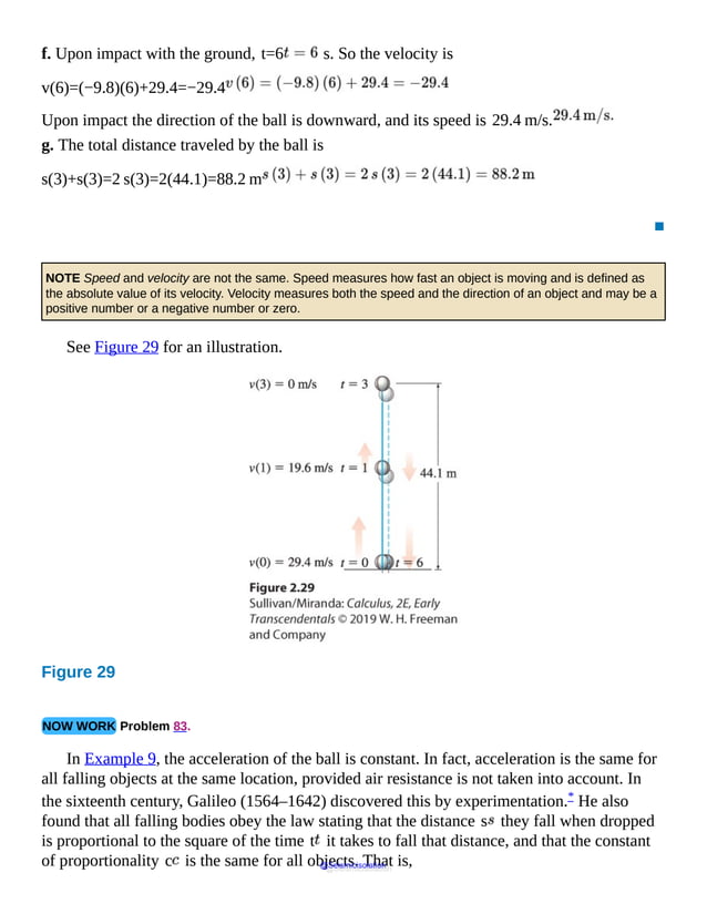
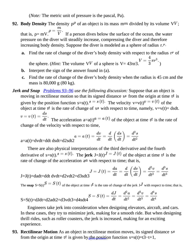
557. b. Find the jerk of a hospital elevator.
Source: Elevator Ride Quality, January 2007, http://www.lift-
report.de/index.php/news/176/368/Elevator-Ride-Quality.
97. Current Density in a Wire The current density J in a wire is a measure of how much
an electricalcurrent is compressed as it flows through a wire and is modeled by the
function J(A)=IA, where I is the current (in amperes) and A is the cross-
sectional area of the wire. In practice, current density, rather than merely current, is
often important. For example, superconductors lose their superconductivity if the
current density is too high.
a. As current flows through a wire, it heats the wire, causing it to expand in area A.
If a constant current is maintained in a cylindrical wire, find the rate of change of
the current density J with respect to the radius r of the wire.
b. Interpret the sign of the answer found in (a).
c. Find the rate of change of current density with respect to the radius r when a
current of 2.5 amps flows through a wire of radius r=0.50 mm.
98. Derivative of a Reciprocal, Function Prove that if a function g is differentiable, then
ddx1g(x)=−g′(x)[g(x)]2, provided g(x)≠0.
99. Extended Product Rule Show that if f,g, and h are differentiable functions, then
ddx[f (x)g(x)h(x)]=f (x)g(x)h′(x)+f (x)g′(x)h(x)+f′(x)g(x)h(x)
From this, deduce that
ddx[f (x)]3=3[f (x)]2f′(x)
In Problems 100–105, use the Extended Product Rule (Problem 99) to find y′ .
100. y=(x2+1)(x−1)(x+5)
101. y=(x−1)(x2+5)(x3−1)
102. y=(x4+1)3
103. y=(x3+1)3
@Seismicisolation
@Seismicisolation

558. 104. y=(3x+1)1+ 1x (x−5+1)
105. y= 1− 1x1−1x21−1x3
106. (Further) Extended Product Rule Write a formula for the derivative of the product of
four differentiable functions. That is, find a formula for ddx[f1(x)f2(x)f3(x)f4(x)].
Also find a formula for ddx[f (x)]4.
107. If f and g are differentiable functions, show that if f (x)= 1f (x)g(x),
then
F′(x)=−f (x)f′(x)f (x)+g′(x)g(x)
provided f (x)≠0, g(x)≠0.
108. Higher-Order Derivatives If f (x)= 11−x, find a formula for the n th
derivative of f. That is, find f(n)(x).
109. Let f (x)= x6−x4+x2x4+1. Rewrite f in the form
(x4+1)f (x)=x6−x4+x2. Now find f′(x) without
using the quotient rule.
110. If f and g are differentiable functions with f≠−g, find the derivative of
fgf+g.
111. f (x)= 2xx+1.
a. Use technology to find f′(x).
b. Simplify f′ to a single fraction using either algebra or a CAS.
c. Use technology to find f(5)(x). (Hint: Your CAS may have a method
for finding higher-order derivatives without finding other derivatives first.)
Challenge Problems
112. Suppose f and g have derivatives up to the fourth order. Find the first four
@Seismicisolation
@Seismicisolation

559. derivatives of the product fg and simplify the answers. In particular, show that the
fourth derivative is
d4dx4⁢(fg)=f(4)g+4f(3)g(1)+6f(2)g(2)+4f(1)g(3)+fg(4)
Identify a pattern for the higher-order derivatives of fg.
113. Suppose f1(x),…,fn(x) are differentiable functions.
a. Find ddx[f1(x)⋅…⋅fn(x)].
b. Find ddx1f1(x)⋅…⋅fn(x).
114. Let a,b,c, and d be real numbers. Define
a bc d=ad−bc
This is called a 2×2 determinant and it arises in the study of linear equations. Let f1(x),f2(x),f3(x),
and f4(x) be differentiable and let
D(x)= f1(x) f2(x)f3(x) f4(x)
Show that
D′(x)= f1′(x) f2′(x)f3(x) f4(x)+ f1(x) f2(x)f3′(x) f4′(x)
115. Let f0(x)=x−1f1(x)=1+ 1x−1f2(x)=1+ 11+1x−1f3(x)=1+ 11+11+1x−1
@Seismicisolation
@Seismicisolation

560. a. Write f1, f2, f3, f4, and f5 in the form ax+bcx+d.
b. Using the results from (a), write the sequence of numbers representing the
coefficients of x in the numerator, beginning with f0(x)=x−1.
c. Write the sequence in (b) as a recursive sequence.
(Hint: Look at the sum of consecutive terms.)
d. Find f0′, f1′, f2′, f3′, f4′, and f5′.
1. = NOW WORK problem
= Graphing technology recommended
= Computer Algebra System recommended
* In a famous legend, Galileo dropped a feather and a rock from the top of the Leaning
Tower of Pisa, to show that the acceleration due to gravity is constant. He expected them to
fall together, but he failed to account for air resistance that slowed the feather. In July 1971,
Apollo 15 astronaut David Scott repeated the experiment on the Moon, where there is no air
resistance. He dropped a hammer and a falcon feather from his shoulder height. Both hit the
Moon’s surface at the same time. A video of this experiment may be found at the NASA
website.
@Seismicisolation
@Seismicisolation

561. 2.5 The Derivative of the Trigonometric Functions
OBJECTIVE When you finish this section, you should be able to:
1 Differentiate trigonometric functions
1 Differentiate Trigonometric Functions
To find the derivatives of y=sin x and y=cos x, we use the limits
limθ→0 sin θθ=1andlimθ→0 cos θ−1θ=0
that were established in Section 1.4.
THEOREM Derivative of y=sin x
The derivative of y=sin x is y′=cos x. That is,
y′=ddx sin x=cos x
Proof
y′=limh→0 sin(x+h)−sin xh The definition of a derivative=limh→0 sin x cos h+sin h cos x
−sin xh sin(A+B)=sin A cos B+sin B cos A=limh→0sin x cos h−sin xh+sin h cos xh
Rearrange terms.=limh→0sin x⋅cos h−1h+sin hh⋅cos x Factor.=limh→0 sin xlimh→0 cos h
−1h+limh→0 cos xlimh→0 sin hhUse properties of
limits.=sin x⋅0+cos x⋅1=cos xlimθ→0 cos θ−1θ=0; limθ→0 sin θθ=1
@Seismicisolation
@Seismicisolation

562. ▪
NEED TO REVIEW? The trigonometric functions are discussed in Section P.6, pp. 52–59. Trigonometric
identities are discussed in Appendix A.4, pp. A-32 to A-35.
The geometry of the derivative ddx sin x=cos x is shown in Figure 30.
On the graph of f(x)=sin x, the horizontal tangents are marked as well as the
tangent lines that have slopes of 1 and −1. The derivative function is plotted on the
second graph and those points are connected with a smooth curve.
Figure 30
On
the
graph
of
f
of
x,
the
horizontal
tangent
lines
To find derivatives involving the trigonometric functions, use the sum, difference,
product, and quotient rules and the derivative formulas from Sections 2.3 and 2.4.
EXAMPLE 1 Differentiating the Sine Function
Find y′ if:
a. y=x+4 sin x
b. y=x2 sin x
c. y=sin xx
@Seismicisolation
@Seismicisolation

563. d. y=ex sin x
Solution a. Use the Sum Rule and the Constant Multiple Rule.
y′=ddx (x+4 sin x)=ddx x+ddx (4 sin x)=1+4 ddx sin x=1+4 cos x
b. Use the Product Rule.
y′=ddx (x2 sin x)=x2ddx sin x+ddx x2 sin x=x2 cos x+2x sin x
c. Use the Quotient Rule.
y′=ddx sin xx=ddx sin x⋅x−sin x⋅ddx xx2=x cos x−sin xx2
d. Use the Product Rule.
y′=ddx (ex sin x)=exddx sin x+ddx ex sin x=ex cos x+ex sin x=ex(cos x+sin x)
▪
NOW WORK Problem 5, 29, and 45.
THEOREM Derivative of y=cos x
The derivative of y=cos x is
y′=ddx cos x=−sin x
You are asked to prove this in Problem 75.
EXAMPLE 2 Differentiating Trigonometric Functions
Find the derivative of each function:
@Seismicisolation
@Seismicisolation

564. a. f(x)=x2 cos x
b. g(θ)=cos θ1−sin θ
c. F(t)=etcos t
Solution
a. f′(x)=ddx (x2 cos x)=x2ddx cos x+ddx x2(cos x)=x2(−sin x)+2x cos x=2x cos x−x2 sin x
b. g′(θ)=ddθ cos θ1−sin θ=ddθ cos θ(1−sin θ)−cos θddθ (1−sin θ)(1−sin θ)2=−sin θ1−sin θ
−cos θ(−cos θ)1−sin θ2=−sin θ+sin2 θ+cos2 θ1−sin θ2=−sin θ+11−sin θ2=11−sin θ
c. F′(t)=ddt etcos t=ddt etcos t−etddt cos tcos2 t=et cos t−et(−sin t)cos2 tF
′(t)=et(cos t+sin t)cos2 t
▪
NOW WORK Problem 13.
EXAMPLE 3 Identifying Horizontal Tangent Lines
Find all points on the graph of f(x)=x+sin x where the tangent line is
horizontal.
@Seismicisolation
@Seismicisolation

565. Solution Since tangent lines are horizontal at points on the graph of f where f′(x)=0,
begin by finding f′(x)=1+cos x.
Now solve the equation: f′(x)=1+cos x=0.
cos x=−1 x=(2k+1)π where k is an integer
At each of the points ((2k+1)π,(2k+1)π), where k is an integer, the
graph of f has a horizontal tangent line. See Figure 31.
Figure 31 f(x)=x+sin x
Notice that each of the points with a horizontal tangent line lies on the line y=x.
▪
NOW WORK Problem 57.
The derivatives of the remaining four trigonometric functions are obtained using
trigonometric identities and basic derivative rules. We establish the formula for the derivative
of y=tan x in Example 4. You are asked to prove formulas for the derivative of the
secant function, the cosecant function, and the cotangent function in the exercises. (See
Problems 76–78.)
EXAMPLE 4 Differentiating y=tan x @Seismicisolation
@Seismicisolation

566. Show that the derivative of y=tan x is
y′=ddx tan x=sec2 x
Solution
▪
NOW WORK Problem 15.
Table 4 lists the derivatives of the six trigonometric functions along with the domain of
each derivative.
TABLE 4
Derivative Function Domain of the Derivative Function
ddx sin x=cos x
(−∞,∞)
ddx cos x=−sin x
(−∞,∞)
ddx tan x=sec2 x
x|x≠2k+12π,k an
integer
ddx cot x=−csc2 x
{x|x≠kπ,k an
integer}
ddx csc x=−csc x cot x
{x|x≠kπ,k an
integer}
ddx sec x=sec x tan x
x|x≠2k+12π,k an
integer
NOTE If the trigonometric function begins with the letter c, that is, cosine, cotangent, or cosecant, then its
derivative has a minus sign.
EXAMPLE 5 Finding the Second Derivative of a Trigonometric Function
@Seismicisolation
@Seismicisolation

567. ▪
NOW WORK Problem 35.
Application: Simple Harmonic Motion
Simple harmonic motion is a repetitive motion that can be modeled by a trigonometric
function. A swinging pendulum and an oscillating spring are examples of simple harmonic
motion.
EXAMPLE 6 Analyzing Simple Harmonic Motion
An object hangs on a spring, making the spring 2 m long in its equilibrium position. See
Figure 32. If the object is pulled down 1 m and released, it oscillates up and down. The
length l of the spring after t seconds is modeled by the function l(t)=2+cos t.
Figure 32
a. How does the length of the spring vary?
@Seismicisolation
@Seismicisolation

568. b. Find the velocity of the object.
c. At what position is the speed of the object a maximum?
d. Find the acceleration of the object.
e. At what position is the acceleration equal to 0 ?
Solution a. Since l(t)=2+cos t and −1≤cos t≤1, the length of
the spring oscillates between 1 and 3 m.
b. The velocity v of the object is
v=l′(t)=ddt 2+cos t=−sin t
c. Speed is the magnitude of velocity. Since v=−sin t, the speed of the object is v=
−sin t=sin t. Since −1≤sin t≤1, the object moves the
fastest when v=sin t=1. This occurs when sin t=±1 or,
equivalently, when cos t=0. So, the speed is a maximum when l(t)=2, that
is, when the spring is at the equilibrium position.
d. The acceleration a of the object is given by
a=l″(t)=ddt l′(t)=ddt (−sin t)=−cos t
(e) Since a=−cos t, the acceleration is zero when cos t=0. So, a=0
when l(t)=2, that is, when the spring is at the equilibrium position. This is the same
time at which the speed is maximum. ▪
Figure 33 shows the graphs of the length of the spring y=l(t), the velocity
y=v(t), and the acceleration y=a(t).
@Seismicisolation
@Seismicisolation

569. Figure 33
NOW WORK Problem 65.
2.5 Assess Your Understanding
Concepts and Vocabulary
1. True or False ddx cos x=sin x
2. True or False ddx tan x=cot x
3. True or False d2dx2 sin x=−sin x
4. True or False ddx sin π3=cos π3
Skill Building
In Problems 5–38, find y′.
5. y=x−sin x
6. y=cos x−x2
7. y=tan x+cos x
@Seismicisolation
@Seismicisolation

570. 8. y=sin x−tan x
9. y=3 sin θ−2 cos θ
10. y=4 tan θ+sin θ
11. y=sin x cos x
12. y=cot x tan x
13. y=t cos t
14. y=t2 tan t
15. y=ex tan x
18. y=π u tan u
19. y=cot xx
20. y=csc xx
21. y=x2 sin x
22. y=t2 tan t
25. y=sin θ1−cos θ
26. y=xcos x
27. y=sin t1+t
28. y=tan u1+u
29. y=sin xex
30. y=cos xex
31. y=sin θ+cos θsin θ−cos θ
32. y=sin θ−cos θsin θ+cos θ
@Seismicisolation
@Seismicisolation

571. 34. y=csc t1+t cos t
35. y=csc θ cot θ
36. y=tan θ cos θ
37. y=1+tan x1−tan x
38. y=csc x−cot xcsc x+cot x
In Problems 39–50, find y″ .
39. y=sin x
40. y=cos x
41. y=tan θ
42. y=cot θ
43. y=t sin t
44. y=t cos t
45. y=ex sin x
46. y=ex cos x
47. y=2 sin u−3 cos u
48. y=3 sin u+4 cos u
49. y=a sin x+b cos x
In Problems 51–56:
a. Find an equation of the tangent line to the graph of f at the indicated point.
b. Graph the function and the tangent line.
51. f (x)=sin x at (0,0)
52. f (x)=cos x at π3,12
53. f (x)=tan x at (0,0)
54. f (x)=tan x at π4,1
@Seismicisolation
@Seismicisolation

572. 55. f (x)=sin x+cos x at π4,2
56. f (x)=sin x−cos x at π4,0
In Problems 57–60:
a. Find all points on the graph of f where the tangent line is horizontal.
b. Graph the function and the horizontal tangent lines on the interval [−2π,2π] .
57. f (x)=2 sin x+cos x
58. f (x)=cos x−sin x
60. f (x)=csc x
Applications and Extensions
In Problems 61 and 62, find the nth derivative of each function.
61. f (x)=sin x
62. f (θ)=cos θ
63. What is limh→0 cos π2+h−cos π2h?
64. What is limh→0 sin(π+h)−sin πh ?
65. Simple Harmonic Motion The signed distance s (in meters) of an object from the
origin at time t (in seconds) is modeled by the position function s(t)=18 cos t.
a. Find the velocity v of the object.
b. When is the speed of the object a maximum?
c. Find the acceleration a of the object.
d. When is the acceleration equal to 0 ?
e. Graph s, v, and a on the same screen.
66. Simple Harmonic Motion An object attached to a coiled spring is pulled down a
distance d=5 cm from its equilibrium position and then released as shown in the
figure. The motion of the object at time t seconds is simple harmonic and is modeled
@Seismicisolation
@Seismicisolation

573. by d(t)=−5 cos t.
a. As t varies from 0 to 2π, how does the length of the spring vary?
b. Find the velocity v of the object.
c. When is the speed of the object a maximum?
d. Find the acceleration a of the object.
e. When is the acceleration equal to 0 ?
f. Graph d, v, and a on the same screen.
67. Rate of Change A large, 8-ft high decorative mirror is placed on a wood floor and
leaned against a wall. The weight of the mirror and the slickness of the floor cause the
mirror to slip.
a. If θ is the angle between the top of the mirror and the wall, and y is the distance
from the floor to the top of the mirror, what is the rate of change of y with respect
to θ?
b. In feet/radian, how fast is the top of the mirror slipping down the wall when θ=π4?
68. Rate of Change The sides of an isosceles triangle are sliding outward. See the Figure.
a. Find the rate of change of the area of the triangle with respect to θ.
b. How fast is the area changing when θ=π6?
@Seismicisolation
@Seismicisolation

574. 69. Sea Waves Waves in deep water tend to have the symmetric form of the function
f(x)=sin x. As they approach shore, however, the sea floor creates drag,
which changes the shape of the wave. The trough of the wave widens and the height of
the wave increases, so the top of the wave isno longer symmetric with the trough. This
type of wave can be represented by a function such as
w(x)=42+cos x
a. Graph w=w(x) for 0≤x≤4π.
b. What is the maximum and the minimum value of w ?
c. Find the values of x, 0<x<4π, at which w′(x)=0.
d. Evaluate w′ near the peak at π, using x=π−0.1, and near the trough
at 2π, using x=2π−0.1.
e. Explain how these values confirm a nonsymmetric wave shape.
70. Swinging Pendulum A simple pendulum is a small-sized ball swinging from a light
string. As it swings, the supporting string makes an angle θ with the vertical. See the
figure. At an angle θ, the tension in the string is T=Wcos θ, where W is
the weight of the swinging ball.
a. Find the rate of change of the tension T with respect to θ when the pendulum is
at its highest point (θ=θmax).
b. Find the rate of change of the tension T with respect to θ when the pendulum is
at its lowest point.
c. What is the tension at the lowest point?
@Seismicisolation
@Seismicisolation

575. 71. Restaurant Sales A restaurant in Naples, Florida is very busy during the winter months
and extremely slow over the summer. But every year the restaurant grows its sales.
Suppose over the next two years, the revenue R, in units of $10,000, is projected to
follow the model
R=R(t)=sin t+0.3t+10≤t≤12
where t=0 corresponds to November 1, 2018; t=1 corresponds to January 1,
2019; t=2 corresponds to March 1, 2019; and so on.
a. What is the projected revenue for November 1, 2018; March 1, 2019; September 1,
2019; and January 1, 2020?
b. What is the rate of change of revenue with respect to time?
c. What is the rate of change of revenue with respect to time for January 1, 2020?
d. Graph the revenue function and the derivative function R′=R′(t).
e. Does the graph of R support the facts that every year the restaurant grows its
sales and that sales are higher during the winter and lower during the summer?
Explain.
72. Polarizing Sunglasses Polarizing sunglasses are filters that transmit only light for
which the electric field oscillations are in a specific direction. Light is polarized
naturally by scattering off the molecules in the atmosphere and by reflecting off many
(but not all) types of surfaces. If light of intensity I0 is already polarized in a certain
direction, and the transmission direction of the polarizing filter makes an angle with that
direction, then the intensity I of the light after passing through the filter is given by
Malus’s Law, I(θ)=I0 cos2 θ.
a. As you rotate a polarizing filter, θ changes. Find the rate of change of the light
intensity I with respect to θ.
@Seismicisolation
@Seismicisolation

576. b. Find both the intensity I(θ) and the rate of change of the intensity with respect
to θ, for the angles θ=0 ∘, 45 ∘, and 90 ∘. (Remember to use
radians for θ.)
73. If y=sin x and y(n) is the n th derivative of y with respect to x, find
the smallest positive integer n for which y(n)=y.
74. Use the identity sin A−sin B=2 cos A+B2 sin A−B2,
with A=x+h and B=x, to
prove that
ddx sin x=limh→0 sin(x+h)−sin xh=cos x
75. Use the definition of a derivative to prove ddx cos x=−sin x.
76. Derivative of y=sec x Use a derivative rule to show that
77. Derivative of y=csc x Use a derivative rule to show that
ddx csc x=−csc x cot x
78. Derivative of y=cot x Use a derivative rule to show that
ddx cot x=−csc2 x
79. Let f (x)=cos x. Show that finding f′(0) is the same as finding
limx→0 cos x−1x.
80. Let f (x)=sin x. Show that finding f′(0) is the same as finding
limx→0 sin xx. @Seismicisolation
@Seismicisolation

577. 81. If y=A sin t+B cos t, where A and B are constants, show that
y″+y=0.
Challenge Problem
82. For a differentiable function f, let f* be the function defined by
f*(x)=limh→0 f(x+h)−f(x−h)h
a. Find f*(x) for f (x)=x2+x.
b. Find f*(x) for f (x)=cos x.
c. Write an equation that expresses the relationship between the functions f* and f′,
where f′ denotes the derivative of f. Justify your answer.
1. = NOW WORK problem
= Graphing technology recommended
= Computer Algebra System recommended
@Seismicisolation
@Seismicisolation

578. Chapter Review
THINGS TO KNOW
2.1 Rates of Change and the Derivative
Definition Derivative of a function at a number f′(c)=limx→c f (x)−f (c)x−c
provided the limit exists. (p. 159)
Three Interpretations of the Derivative
Geometric If y=f (x), the derivative f′(c) is the slope of the tangent line
to the graph of f at the point (c,f (c)). (p. 154)
Rate of change of a function If y=f (x), the derivative f′(c) is the rate
of change of f with respect to x at c. (p. 156)
Physical If the signed distance s from the origin at time t of an object in rectilinear
motion is given by the position function s=f (t), the derivative f′(t0) is
the velocity of the object at time t0. (p. 158)
2.2 The Derivative as a Function
Definition of a derivative function (Form 3) (p. 164) f′(x)=limh→0 f (x+h)−f (x)h,
provided the limit exists.
Theorem If a function f has a derivative at a number c, then f is continuous at c.
(p. 169)
Corollary If a function f is discontinuous at a number c, then f has no derivative
at c. (p. 169)
2.3 The Derivative of a Polynomial Function; The Derivative of y=ex
Leibniz notation dydx=ddx y=ddx f (x) (p. 174)
Basic derivatives ddx A=0 A is a constant (p. 175) ddx x=1 (p.
175) ddx ex=ex (p. 181)
Simple Power Rule ddx xn=nxn−1, n≥1, an integer (p. 176)
@Seismicisolation
@Seismicisolation

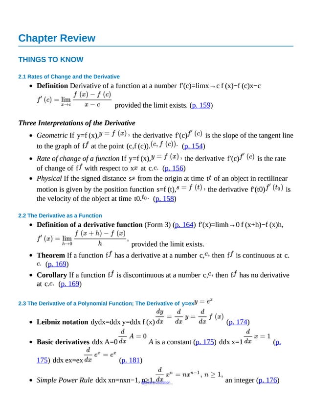
579. Properties of Derivatives
Sum Rule (p. 177) ddx[f+g]=ddx f+ddx g(f+g)′=f′+g′
Difference Rule (p. 178) ddx[f−g]=ddx f−ddx g(f−g)′=f′−g′
Constant Multiple Rule If k is a constant, (p. 177) ddx[kf]=k ddx f(kf)′=k⋅f′
2.4 Differentiating the Product and the Quotient of Two Functions; Higher-Order Derivatives
Properties of Derivatives
Product Rule (p. 185) ddx(fg)=fddx g+ddx fg(fg)′=fg′+f′g
Quotient Rule (p. 186) ddx fg=ddx fg−f ddx gg2fg′=f′g−fg′g2
provided g(x)≠0
Reciprocal Rule (p. 187) ddx 1g=−ddx gg21g′=−g′g2 provided
g(x)≠0
Power Rule ddx xn=nxn−1, n an integer (p. 188)
Higher-order derivatives See Table 3 (p. 189)
Position Function s=s(t)
@Seismicisolation
@Seismicisolation

580. Velocity v=v(t)= dsdt
Acceleration a=a(t)= dvdt=d2sdt2 (p. 190)
2.5 The Derivative of the Trigonometric Functions
Basic Derivatives
ddx sin x=cos x (p. 196)
ddx cos x=−sin x (p. 198)
ddx tan x=sec2x (p. 199)
ddx sec x=sec x tan x (p. 199)
ddx csc x=−csc x cot x (p. 199)
ddx cot x=−csc2x (p. 199)
OBJECTIVES
Section You should be able to … Examples Review Exercises
2.1 1 Find equations for the tangent line and the normal line to the
graph of a function (p. 155)
1 67–70
2 Find the rate of change of a function (p. 156) 2, 3 1, 2, 73 (a)
3 Find average velocity and instantaneous velocity (p. 157) 4, 5 71(a), (b); 72(a), (b)
4 Find the derivative of a function at a number (p. 159) 6–8 3–8, 75
2.2 1 Define the derivative function (p. 163) 1–3 9–12, 77
2 Graph the derivative function (p. 165) 4, 5 9–12, 15–18
3 Identify where a function has no derivative (p. 167) 6–10 13, 14, 75
2.3 1 Differentiate a constant function (p. 175) 1
2 Differentiate a power function (p. 175) 2, 3 19–22
3 Differentiate the sum and the difference of two functions (p. 177) 4–6 23–26, 33, 34, 40, 51,
52, 67
4 Differentiate the exponential function y=ex (p. 180) 7 44, 45, 53, 54, 56, 59, 69
2.4 1 Differentiate the product of two functions (p. 184) 1, 2 27, 28, 36, 46, 48–50,
53–56, 60
2 Differentiate the quotient of two functions (p. 186) 3–6 29–35, 37–43, 47, 57–
59, 68, 73, 74
@Seismicisolation
@Seismicisolation

581. 3 Find higher-order derivatives (p. 189) 7, 8 61–66, 71, 72, 76
4 Work with acceleration (p. 190) 9 71, 72, 76
2.5 1 Differentiate trigonometric functions (p. 196) 1–6 49–60, 70
REVIEW EXERCISES
In Problems 1 and 2, use a definition of the derivative to find the rate of change of f at the
indicated numbers.
1. f (x)=x at
a. c=1
b. c=4
c. c any positive real number
2. f (x)= 2x−1 at
a. c=0
b. c=2
c. c any real number, c≠1
In Problems 3–8, use a definition of the derivative to find the derivative of each function at
the given number.
3. f (x)=2x+5 at 2
4. f (x)=4x2+1 at −1
5. f (x)=3x2+5x at 0
6. f (x)=3x at 1
7. f (x)=4x+1 at 0
8. f (x)=x+12x−3 at 1
In Problems 9–12, use a definition of the derivative to find the derivative of each function.
Graph f and f′ on the same set of axes.
9. f (x)=x−6 @Seismicisolation
@Seismicisolation

582. 10. f (x)=7−3x2
11. f (x)=12x3
12. f (x)=π
In Problems 13 and 14, determine whether the function f has a derivative at c. If it does, find
the derivative. If it does not, explain why. Graph each function.
13. f (x)= |x3−1| at c=1
14. f (x)= 4−3x2 if x≤−1−x3 if x>−1 at c=−1
In Problems 15 and 16, determine if the graphs represent a function f and its derivative f′.
If they do, indicate which is the graph of f and which is the graph of f′.
15.
16.
@Seismicisolation
@Seismicisolation

583. 17. Use the information in the graph of y=f (x) to sketch the graph of y=f′(x).
Tangent
lines
at
points
(minus
4,
2),
(minus
2,
1)
and
18. Match the graph of y=f (x) with the graph of its derivative.
@Seismicisolation
@Seismicisolation

584. @Seismicisolation
@Seismicisolation

585. In Problems 19–60, find the derivative of each function. Where a or b appears, it is a
constant.
19. f (x)=x5
20. f (x)=ax3
21. f (x)=x44
22. f (x)=−6x2
23. f (x)=2x2−3x
24. f (x)=3x3+23 x2−5x+7
25. f (x)=7(x2−4)
26. f (x)=5(x+6)7
27. f (x)=5(x2−3x)(x−6)
28. f (x)=(2x3+x)(x2−5)
29. f (x)=6x4−9x23x3
30. f (x)=2x+25x−3
@Seismicisolation
@Seismicisolation

586. 31. f (x)=7xx−5
32. f (x)=2x−12
33. f (x)=2x2−5x−2
34. f (x)=2+3x+4x2
35. f (x)=ax−bx3
36. f (x)=(x3−1)2
37. f (x)=3(x2−3x)2
38. f (x)=x2x+1
39. s(t)=t3t−2
40. f (x)=3x−2+2x−1+1
41. f (z)=1z2+1
42. f (v)=v−1v2+1
43. g(z)= 11−z+z2
44. f (x)=3ex+x2
45. s(t)=1−et
46. f (x)=aex(2x2+7x)
47. f (x)=1+xex
48. f (x)=(2xex)2
49. f (x)=x sin x
@Seismicisolation
@Seismicisolation

587. 50. s(t)=cos2t
51. G(u)=tan u+sec u
52. g(v)=sin v−13 cos v
53. f (x)=exsin x
54. f (x)=ex csc x
55. f (x)=2 sin x cos x
56. f (x)=(ex+b)cos x
57. f (x)=sin xcsc x
58. f (x)=1−cot x1+cot x
59. f (θ)=cos θ2eθ
60. f (θ)=4θ cot θ tan θ
In Problems 61–66, find the first derivative and the second derivative of each function.
61. f (x)=(5x+3)2
62. f (x)=xex
63. g(u)=u2u+1
64. f (x)=ex(sin x+2 cos x)
65. f (u)=cos ueu
66. f (x)=sin xx
In Problems 67–70, for each function:
a. Find an equation of the tangent line to the graph of the function at the indicated point.
b. Find an equation of the normal line to the function at the indicated point.
c. Graph the function, the tangent line, and the normal line on the same screen.
@Seismicisolation
@Seismicisolation

588. 67. f (x)=2x2−3x+7 at (−1,12)
68. y= x2+12x−1 at 2,53
69. f (x)=x2−ex at (0,−1)
70. s(t)=1+2 sin t at (π,1)
71. Rectilinear Motion As an object in rectilinear motion moves, its signed distance s
(in meters) from the origin at time t (in seconds) is given by the position function
s=f (t)=t2−6t
a. Find the average velocity of the object from 0 to 5 s.
b. Find the velocity at t=0, at t=5, and at any time t.
c. Find the acceleration at any time t.
72. Rectilinear Motion As an object in rectilinear motion moves, its signed distance s
from the origin at time t is given by the position function s(t)=t−t2,
where s is in centimeters and t is in seconds.
a. Find the average velocity of the object from 1 to 3 s.
b. Find the velocity of the object at t=1 s and t=3 s.
c. What is its acceleration at t=1 and t=3 ?
73. Business The price p in dollars per pound when x pounds of a commodity are
demanded is modeled by the function p(x)=10,0005x+100−5,
when between 0 and 90 lb are demanded (purchased).
a. Find the rate of change of price with respect to demand.
b. What is the revenue function R ? (Recall, revenue R equals price times amount
purchased.)
c. What is the marginal revenue R′ at x=10 and at x=40 lb?
74. If f (x)= x−1x+1 for all x≠−1, find f′(1).
75. If f (x)=2+ |x−3| for all x, determine whether the derivative f′
exists at x=3.
76. Rectilinear Motion An object in rectilinear motion moves according to the position
function s=2t3−15t2+24t+3, where t is measured in minutes
@Seismicisolation
@Seismicisolation

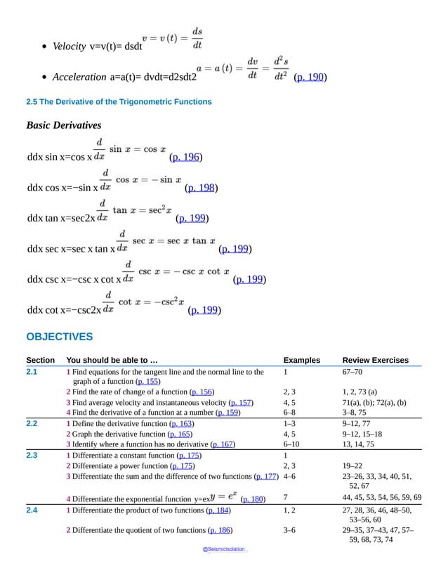
589. and s in meters.
a. When is the object at rest?
b. Find the object’s acceleration when t=3.
77. Find the value of the limit below and specify the function f for which this is the
derivative.
limΔx→0 [4−2(x+Δx)]2−(4−2x)2Δx
@Seismicisolation
@Seismicisolation

590. (1)
CHAPTER 2 PROJECT The Lunar Module
The Lunar Module (LM) was a small spacecraft that detached from the Apollo Command
Module and was designed to land on the Moon. Fast and accurate computations were
needed to bring the LM from an orbiting speed of about 5500 ft/s to a speed slow enough
to land it within a few feet of a designated target on the Moon’s surface. The LM carried a
70-lb computer to assist in guiding it successfully to its target. The approach to the target
was split into three phases, each of which followed a reference trajectory specified by
NASA engineers.* The position and velocity of the LM were monitored by sensors that
tracked its deviation from the preassigned path at each moment. Whenever the LM strayed
from the reference trajectory, control thrusters were fired to reposition it. In other words,
the LM’s position and velocity were adjusted by changing its acceleration.
The reference trajectory for each phase was specified by the engineers to have the form
rref(t)=RT+VTt+12ATt2+16JTt3+124STt4
The variable rref represents the intended position of the LM at time t before the end
of the landing phase. The engineers specified the end of the landing phase to take place at
t=0, so that during the phase, t was always negative. Note that the LM was landing
in three dimensions, so there were actually three equations like (1). Since each of those
equations had this same form, we will work in one dimension, assuming, for example, that
r represents the distance of the LM above the surface of the Moon.
@Seismicisolation
@Seismicisolation

591. (2)
1. If the LM follows the reference trajectory, what is the reference velocity vref(t) ?
2. What is the reference acceleration aref(t) ?
3. The rate of change of acceleration is called jerk. Find the reference jerk Jref(t).
4. The rate of change of jerk is called snap. Find the reference snap Sref(t).
5. Evaluate rref(t), vref(t), aref(t), Jref(t), and Sref(t)
when t=0.
The reference trajectory given in equation (1) is a fourth-degree polynomial, the lowest
degree polynomial that has enough free parameters to satisfy all the mission criteria. Now
we see that the parameters RT=rref(0), VT=vref (0), AT=aref
(0), JT=Jref(0), and ST=Sref(0). The five
parameters in equation (1) are referred to as the target parameters since they provide the
path the LM should follow.
But small variations in propulsion, mass, and countless other variables cause the LM to
deviate from the predetermined path. To correct the LM’s position and velocity, NASA
engineers apply a force to the LM using rocket thrusters. That is, they changed the
acceleration. (Remember Newton’s second law, F=ma.) Engineers modeled the
actual trajectory of the LM by
r(t)=RT+VTt+12ATt2+16JAt3+124SAt4
We know the target parameters for position, velocity, and acceleration. We need to find the
actual parameters for jerk and snap to know the proper force (acceleration) to apply.
6. Find the actual velocity v=v(t) of the LM.
7. Find the actual acceleration a=a(t) of the LM.
8. Use equation (2) and the actual velocity found in Problem 6 to express JA and SA
in terms of RT, VT, AT, r(t), and v(t).
9. Use the results of Problems 7 and 8 to express the actual acceleration a=a(t) in
terms of RT, VT, AT, r(t), and v(t).
The result found in Problem 9 provides the acceleration (force) required to keep the LM in
its reference trajectory.
10. When riding in an elevator, the sensation one feels just before the elevator stops at a
floor is jerk. Would you want jerk to be small or large in an elevator? Explain. Would
you want jerk to be small or large on a roller coaster ride? Explain. How would you
explain snap? @Seismicisolation
@Seismicisolation

592. _________________
*A. R. Klumpp, “Apollo Lunar-Descent Guidance,” MIT Charles Stark Draper Laboratory,
R-695, June 1971, http://www.hq.nasa.gov/alsj/ApolloDescentGuidnce.pdf.
@Seismicisolation
@Seismicisolation

593. 3 More About Derivatives
3.1 The Chain Rule
3.2 Implicit Differentiation
3.3 Derivatives of the Inverse Trigonometric Functions
3.4 Derivatives of Logarithmic Functions
3.5 Differentials; Linear Approximations; Newton’s Method
3.6 Hyperbolic Functions
Chapter Review
Chapter Project
World Population Growth
In the late 1700s Thomas Malthus predicted that population growth, if left
unchecked, would outstrip food resources and lead to mass starvation. His
prediction turned out to be incorrect, since in 1800 world population had not yet
reached one billion and currently world population is in excess of seven billion.
Malthus’ most dire predictions did not come true largely because improvements in
food production made his models inaccurate. On the other hand, his population
growth model is still used today, and population growth remains an important issue
in human progress. For example, many people are crowded into growing urban
@Seismicisolation
@Seismicisolation

594. areas, such as India’s Kolkata (pictured above), which has a population of over
14.3 million and a density of over 63,000 people per square mile.
CHAPTER 3 PROJECT In the Chapter Project on page 261, we explore a basic
model to predict world population and examine its accuracy.
In this chapter, we continue exploring properties of derivatives, beginning with the Chain
Rule, which allows us to differentiate composite functions. The Chain Rule also provides the
means to establish derivative formulas for exponential functions, logarithmic functions, and
hyperbolic functions.
We also solve problems involving relative error in the measurements of two related
variables and use the derivative to approximate the real zeros of a function.
@Seismicisolation
@Seismicisolation

595. 3.1 The Chain Rule
OBJECTIVES When you finish this section, you should be able to:
1 Differentiate a composite function
2 Differentiate y=ax, a>0, a≠1
3 Use the Power Rule for functions to find a derivative
4 Use the Chain Rule for multiple composite functions
Using the differentiation rules developed so far, it would be difficult to differentiate the
function
F(x)=(x3−4x+1)100
But F is the composite function of f(u)=u100 and u=g(x)=x3−4x+1,
so F(x)=f(g(x))=(f∘g)(x)=(x3−4x+1)100.
In this section, we derive the Chain Rule,
a result that enables us to find the derivative of a composite function. We use the Chain Rule
to find the derivative in applications involving functions such as A(t)=102−90e−0.21t
(market penetration, Problem 101) and v(t)=mgk (1−e−kt⁄m)
(the terminal velocity of a falling object, Problem 103).
NEED TO REVIEW? Composite functions and their properties are discussed in Section P.3, pp. 27–29.
1 Differentiate a Composite Function
Suppose y=(f∘g)(x)=f(g(x)) is a composite function, where y=f(u)
is a differentiable function of u, and u=g(x) is a differentiable function
of x. What is the derivative of (f∘g)(x) ? It turns out that the derivative of the
composite function f∘g is the product of the derivatives f′(u)=f′(g(x))
and g′(x).
THEOREM Chain Rule
If a function g is differentiable at x and a function f is differentiable at g(x), then
the composite function f∘g is differentiable at x and
@Seismicisolation
@Seismicisolation

596. (f∘g)′(x)=f′(g(x))⋅g′(x)
For differentiable functions y=f(u) and u=g(x), the Chain Rule, in
Leibniz notation, takes the form
dydx=dydu⋅dudx
where in dydu we substitute u=g(x).
IN WORDS If you think of the function y=f(u) as the outside function and the function u=g(x)
as the inside function, then the derivative of f∘g is the derivative of the outside function,
evaluated at the inside function, times the derivative of the inside function. That is,
ddx (f∘g)(x)=f′(g(x))⋅g′(x)
Partial Proof The Chain Rule is proved using the definition of a derivative. first we observe
that if x changes by a small amount Δx, the corresponding change in u=g(x)
is Δu and Δu depends on Δx. Also,
g′(x)=dudx=limΔx→0 ΔuΔx
Since y=f(u), the change Δu, which could equal 0, causes a change Δy.
Suppose Δu is never 0. Then
f′(u)=dydu=limΔu→0 ΔyΔu
To find dydx, we write
Since the differentiable function u=g(x) is continuous, Δu→0 as Δx→0,
so in the first factor we can replace Δx→0 by Δu→0. Then
dydx=limΔu→0 ΔyΔulimΔx→0 ΔuΔx=dydu⋅dudx
@Seismicisolation
@Seismicisolation

597. This proves the Chain Rule if Δu is never 0. To complete the proof, we need to
consider the case when Δu may be 0. (This part of the proof is given in Appendix B.)
▪
EXAMPLE 1 Differentiating a Composite Function
Find the derivative of:
a. y=(x3−4x+1)100
b. y=cos3x−π4
Solution a. In the composite function y=(x3−4x+1)100, let
u=x3−4x+1. Then y=u100. Now dydu and dudx are
and
dudx=ddx (x3−4x+1)=3x2−4
Now use the Chain Rule to find dydx.
b. In the composite function y=cos3x−π4, let u=3x−π4.
Then y=cos u and
Now use the Chain Rule.
@Seismicisolation
@Seismicisolation

598. ▪
NOW WORK Problems 9 and 37.
EXAMPLE 2 Differentiating a Composite Function
Find y′ if:
a. y=ex2−4
b. y=sin (4ex)
Solution a. For y=ex2−4, let u=x2−4. Then y=eu and
Using the Chain Rule, we get
y′=dydx=dydu⋅dudx=ex2−4⋅2x=2xex2−4
b. For y=sin (4ex), let u=4ex. Then y=sin u and
Using the Chain Rule, we get
y′=dydx=dydu⋅dudx=cos (4ex)⋅4ex=4ex cos (4ex)
▪
For composite functions y=f(u(x)), where f is an exponential or
trigonometric function, the Chain Rule simplifies finding y′. For example,
If y=eu(x), where u=u(x) is a differentiable function of x, then by
the Chain Rule
@Seismicisolation
@Seismicisolation

599. dydx=dydu⋅dudx=eu(x)dudx
That is,
ddx eu(x)=eu(x)dudx
Similarly, if u=u(x) is a differentiable function,
ddx sin u(x)=cos u(x) dudxddx sec u(x)=sec u(x) tan u(x) dudxddx cos u(x)=
−sin u(x) dudxddx csc u(x)=
−csc u(x) cot u(x) dudxddx tan u(x)=sec2u(x) dudxddx cot u(x)=−csc2u(x) dudx
NOW WORK Problem 41.
EXAMPLE 3 Finding an Equation of a Tangent Line
Find an equation of the tangent line to the graph of y=5e4x at the point (0,5).
Solution The slope of the tangent line to the graph of y=f(x) at the point (0,5)
is f′(0).
mtan=f′(0)=20e0=20. Using the point-slope form of a line,
y−5=20(x−0)y−y0=mtan(x−x0)y=20x+5
▪
The graph of y=5e4x and the line y=20x+5 are shown in Figure 1.
@Seismicisolation
@Seismicisolation

600. Figure 1
NOW WORK Problem 77.
EXAMPLE 4 Application: Carbon-14 Dating
All carbon on Earth contains some carbon-14, which is radioactive. When a living organism
dies, the carbon-14 begins to decay at a fixed rate. The formula P(t)=100e−0.000121t
gives the percentage of carbon-14 present at time t years. Notice that
when t=0, the percentage of carbon-14 present is 100%. When the preserved bodies of
15 -year-old La Doncella and two younger children were found in Peru in 2005, 93.5%
of the carbon-14 remained in their bodies, indicating that the three had died about 550
years earlier.
a. What is the rate of change of the percentage of carbon-14 present in a 550 -year-old
fossil? @Seismicisolation
@Seismicisolation

601. b. What is the rate of change of the percentage of carbon-14 present in a 2000 -year-
old fossil?
Solution a. The rate of change of P is given by its derivative
At t=550 years,
P′(550)=−0.0121e−0.000121(550)≈−0.0113
The percentage of carbon-14 present in a 550 -year-old fossil is decreasing at the rate of
1.13% per year.
b. When t=2000 years, the rate of change is
P′(2000)=−0.0121e−0.000121(2000)≈−0.0095
The percentage of carbon-14 present in a 2000 -year-old fossil is decreasing at the rate of
0.95% per year.
▪
NOW WORK Problem 99.
When we stated the Chain Rule, we expressed it two ways: using prime notation and
using Leibniz notation. In each example so far, we have used Leibniz notation. But when
solving numerical problems, using prime notation is often easier. In this form, the Chain Rule
states that if a function g is differentiable at x0 and a function f is differentiable at
g(x0), then
(f∘g)′(x0)=f′(g(x0))g′(x0)
EXAMPLE 5 Differentiating a Composite Function
Suppose h=f∘g. Find h′(1) given that:
f(1)=2f′(1)=1f′(2)=−4g(1)=2g′(1)=−3g′(2)=5
Solution Based on the Chain Rule using prime notation, we have
h′(x0)=(f∘g)′(x0)=f′(g(x0))g′(x0)
@Seismicisolation
@Seismicisolation

602. When x0=1,
▪
NOW WORK Problem 81.
2 Differentiate y=ax, a>0, a≠1
The Chain Rule allows us to establish a formula for differentiating an exponential function
y=ax for any base a>0 and a≠1. We start with the following property of
logarithms:
ax=eln ax=ex ln aa>0,a≠1
Then
NEED TO REVIEW? Properties of logarithms are discussed in Appendix A.1, pp. A-10 to A-11.
THEOREM Derivative of y=ax
The derivative of an exponential function y=ax, where a>0 and a≠1, is
y′=ddx ax=ax ln a
If u=u(x) is a differentiable function, then
ddx au(x)=au(x) ln a dudx
IN WORDS The rate of change of any exponential function y=ax is proportional to the function y
itself.
The second result follows directly from the proof of ddx ax.
@Seismicisolation
@Seismicisolation

603. EXAMPLE 6 Differentiating Exponential Functions
Find the derivative of each function:
a. f(x)=2x
b. F(x)=3−x
c. g(x)=12x2+1
Solution a. f is an exponential function with base a=2.
f′(x)=ddx 2x=2x ln 2ddx ax=ax ln a
b. F′(x)=ddx 3−x=3−x ln 3 ddx (−x)ddx au(x)=au(x) ln a dudx=−3−x ln 3
c. g
′(x)=ddx 12x2+1=12x2+1 ln 12ddx (x2+1)au(x)=au(x) ln a dudx=12x2+1 ln 12⋅(2x)ddx(x2+1)
▪
NOW WORK Problem 47.
3 Use the Power Rule for Functions to Find a Derivative
We use the Chain Rule to establish other derivative formulas, such as a formula for the
derivative of a function raised to a power.
THEOREM Power Rule for Functions
If g is a differentiable function and n is an integer, then
@Seismicisolation
@Seismicisolation

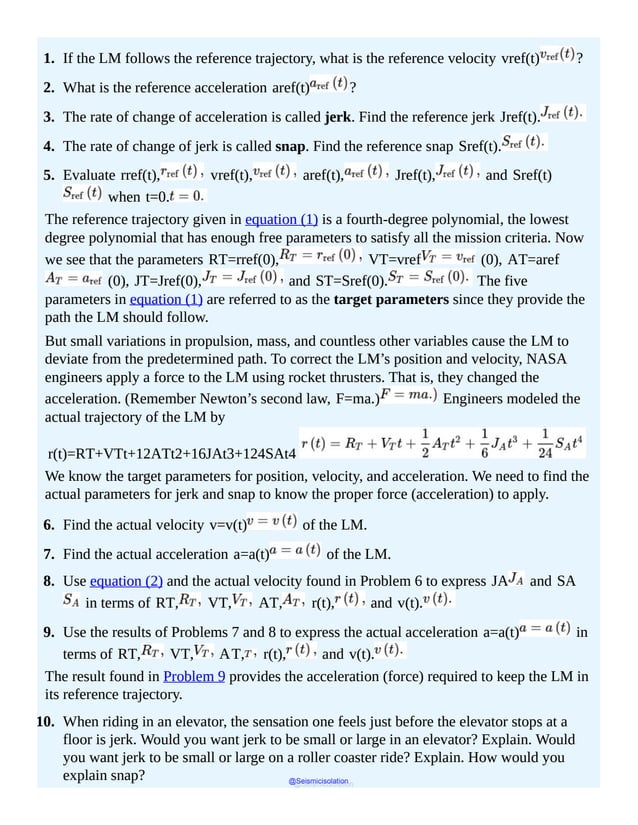
604. ddx [g(x)]n=n[g(x)]n−1g′(x)
Proof If y=[g(x)]n, let y=un and u=g(x). Then
dydu=nun−1=n[g(x)]n−1anddudx=g′(x)
By the Chain Rule,
y′=ddx [g(x)]n=dydu⋅dudx=n[g(x)]n−1g′(x)
▪
EXAMPLE 7 Using the Power Rule for Functions to Find a Derivative
a. If f(x)=(3−x3)−5, then
f′(x)=ddx (3−x3)−5=−5(3−x3)−5−1⋅ddx (3−x3)Use the Power Rule for Functions.=
−5(3−x3)−6⋅(−3x2)=15x2(3−x3)−6=15x2(3−x3)6
b. If f(θ)=cos3 θ, then f(θ)=(cos θ)3, and
f′(θ)=ddθ (cos θ)3=3(cos θ)3−1⋅ddθ cos θUse the Power Rule for Functions.=3 cos2
θ⋅(−sin θ)=−3 cos2 θ sin θ
▪
NOW REWORK Example 7 using the Chain Rule and rework Example 1(a) using the Power Rule for Functions. Decide
for yourself which method is easier.
NOW WORK Problem 21.
@Seismicisolation
@Seismicisolation

605. Often other derivative rules are used along with the Power Rule for Functions.
EXAMPLE 8 Using the Power Rule for Functions with Other Derivative Rules
Find the derivative of:
a. f(x)=ex(x2+1)3
b. g(x)=3x+24x2−55
Solution a. The function f is the product of ex and (x2+1)3, so we first use
the Product Rule.
f′(x)=exddx (x2+1)3+ddx ex(x2+1)3Use the Product Rule.
To complete the solution, we use the Power Rule for Functions to find ddx (x2+1)3.
b. g is a function raised to a power, so we begin with the Power Rule for Functions.
g′(x)=ddx 3x+24x2−55=53x+24x2−54 ddx 3x+24x2−5Use the Power Rule for
Functions.=53x+24x2−54(3)(4x2−5)−(3x+2)(8x)(4x2−5)2Use the Quotient
Rule.=5(3x+2)4[(12x2−15)−(24x2+16x)](4x2−5)6Distribute.=5(3x+2)4[−12x2−16x−15]
(4x2−5)6Simplify.
@Seismicisolation
@Seismicisolation

606. ▪
NOW WORK Problem 29.
4 Use the Chain Rule for Multiple Composite Functions
The Chain Rule can be extended to multiple composite functions. For example, if the
functions
y=f(u)u=g(v)v=h(x)
are each differentiable functions of u, v, and x, respectively, then the composite
function y=(f∘g∘h)(x)=f(g(h(x))) is a differentiable function
of x and
y′=dydx=dydu⋅dudv⋅dvdx
where u=g(v)=g(h(x)) and v=h(x). This “chain” of factors is
the basis for the name Chain Rule.
EXAMPLE 9 Differentiating a Multiple Composite Function
Find y′ if:
a. y=5 cos2 (3x+2)
b. y=sin3 π2 x
@Seismicisolation
@Seismicisolation

607. Solution a. For y=5 cos2(3x+2), use the Chain Rule with y=5u2,
u=cos v, and v=3x+2. Then y=5u2=5 cos2v=5 cos2(3x+2)
and
Then
b. For y=sin3π2 x, use the Chain Rule with y=u3, u=sin v,
and v=π2 x. Then y=u3=(sin v)3=sinπ2 x3=sin3π2 x,
and
Then
▪
NOW WORK Problems 59 and 63.
@Seismicisolation
@Seismicisolation

608. 3.1 Assess Your Understanding
Concepts and Vocabulary
1. The derivative of a composite function (f∘g)(x) can be found using the
______ Rule.
2. True or False If y=f(u) and u=g(x) are differentiable functions,
then y=f(g(x)) is differentiable.
3. True or False If y=f(g(x)) is a differentiable function, then y′=f′(g′(x)).
4. To find the derivative of y=tan (1+cos x), using the Chain Rule,
begin with y=______ and u=______.
5. If y=(x3+4x+1)100, then y′=______.
6. If f(x)=e3x2+5, then f′(x)=______.
7. True or False The Chain Rule can be applied to multiple composite functions.
8. ddx sin x2=______.
Skill Building
In Problems 9–14, write y as a function of x . Find dydx using the Chain Rule.
9. y=u5, u=x3+1
10. y=u3, u=2x+5
11. y=uu+1, u=x2+1
12. y=u−1u, u=x2−1
13. y=(u+1)2, u=1x
14. y=(u2−1)3, u=1x+2
@Seismicisolation
@Seismicisolation

609. In Problems 15–32, find the derivative of each function using the Power Rule for Functions.
15. f(x)=(3x+5)2
16. f(x)=(2x−5)3
17. f(x)=(6x−5)−3
18. f(t)=(4t+1)−2
19. g(x)=(x2+5)4
20. F(x)=(x3−2)5
21. f(u)=u−1u3
22. f(x)=x+1x3
23. g(x)=(4x+ex)3
24. F(x)=(ex−x2)2
25. f(x)=tan2x
26. f(x)=sec3x
27. f(z)=(tan z+cos z)2
28. f(z)=(ez+2 sin z)3
29. y=(x2+4)2(2x3−1)3
30. y=(x2−2)3(3x4+1)2
31. y=sin xx2
32. y=x+cos xx5
In Problems 33–54, find y′ .
@Seismicisolation
@Seismicisolation

610. 33. y=sin (4x)
34. y=cos (5x)
35. y=2 sin (x2+2x−1)
36. y=12 cos (x3−2x+5)
37. y=sin 1x
38. y=sin 3x
39. y=sec (4x)
40. y=cot (5x)
41. y=e1⁄x
42. y=e1⁄x2
43. y=1x4−2x+1
44. y=3x5+2x2−3
45. y=1001+99e−x
46. y=11+2e−x
47. y=2sin x
48. y=(3)cos x
49. y=6sec x
50. y=3tan x
51. y=5xe3x
52. y=x3 e2x
53. y=x2 sin (4x)
@Seismicisolation
@Seismicisolation

611. 54. y=x2 cos (4x)
In Problems 55–58, find y′ (a and b are constants).
55. y=e−axsin (bx)
56. y=eaxcos (−bx)
57. y=eax−1eax+1
58. y=e−ax+1ebx−1
In Problems 59–62, write y as a function of x. Find dydx using the Chain Rule.
59. y=u3, u=3v2+1, v=4x2
60. y=3u, u=3v2−4, v=1x
61. y=u2+1, u=4v, v=x2
62. y=u3−1, u=−2v, v=x3
In Problems 63–70, find y′ .
63. y=e−2x cos (3x)
64. y=eπx tan (πx)
65. y=cos (ex2)
66. y=tan (ex2)
67. y=ecos (4x)
68. y=ecsc2 x
69. y=4 sin2(3x)
@Seismicisolation
@Seismicisolation

612. 70. y=2 cos2(x2)
In Problems 71 and 72, find the derivative of each function by:
a. Using the Chain Rule.
b. Using the Power Rule for Functions.
c. Expanding and then differentiating.
d. Verify the answers from parts (a)–(c) are equal.
71. y=(x3+1)2
72. y=(x2−2)3
In Problems 73–78:
a. Find an equation of the tangent line to the graph of f at the given point.
b. Find an equation of the normal line to the graph of f at the given point.
c. Use technology to graph f, the tangent line, and the normal line on the same screen.
73. f(x)=(x2−2x+1)5 at (1,0)
74. f(x)=(x3−x2+x−1)10 at (0,1)
75. f(x)=x(x2−1)3 at 2,227
76. f(x)=x2(x2−1)2 at 2,49
77. f(x)=sin (2x)+cos x2 at (0,1)
78. f(x)=sin2 x+cos3 x at π2,1
In Problems 79 and 80, find the indicated derivative.
79. d2dx2 cos (x5)
80. d3dx3 sin3x
@Seismicisolation
@Seismicisolation

613. 81. Suppose h=f∘g. Find h′(1) if f′(2)=6, f(1)=4,
g(1)=2, and g′(1)=−2.
82. Suppose h=f∘g. Find h′(1) if f′(3)=4, f(1)=1,
g(1)=3, and g′(1)=3.
83. Suppose h=g∘f. Find h′(0) if f(0)=3, f′(0)=−1,
g(3)=8, and g′(3)=0.
84. Suppose h=g∘f. Find h′(2) if f(1)=2, f′(1)=4, f(2)=
−3, f′(2)=4,g(−3)=1, and g′(−3)=3.
85. If y=u5+u and u=4x3+x−4, find dydx at x=1.
86. If y=eu+3u and u=cos x, find dydx at x=0.
Applications and Extensions
In Problems 87–94, find the indicated derivative.
87. ddx f(x2+1) ( Hint: Let u=x2+1. )
88. ddxf(1−x2)
89. ddxfx+1x−1
90. ddxf1−x1+x
91. ddx f(sin x)
92. ddx f(tan x)
93. d2dx2 f(cos x)
94. d2dx2f(ex)
@Seismicisolation
@Seismicisolation

614. 95. Rectilinear Motion An object is in rectilinear motion and its position s, in meters,
from the origin at time t seconds is given by s=s(t)=A cos (ωt+ϕ
), where A, ω, and ϕ are constants.
a. Find the velocity v of the object at time t.
b. When is the velocity of the object 0 ?
c. Find the acceleration a of the object at time t.
d. When is the acceleration of the object 0?
96. Rectilinear Motion A bullet is fired horizontally into a bale of paper. The distance s
(in meters) the bullet travels into the bale of paper in t seconds is given by
s=s(t)=8−(2−t)30≤t≤2
a. Find the velocity v of the bullet at any time t.
b. Find the velocity of the bullet at t=1.
c. Find the acceleration a of the bullet at any time t.
d. Find the acceleration of the bullet at t=1.
e. How far into the bale of paper did the bullet travel?
97. Rectilinear Motion Find the acceleration a of a car if the distance s, in feet, it has
traveled along a highway at time t≥0 seconds is given by
s(t)=803 t+3π sinπ6 t
98. Rectilinear Motion An object moves in rectilinear motion so that at time t≥0
seconds, its position from the origin is s(t)=sin et, in feet.
a. Find the velocity v and acceleration a of the object at any time t.
b. At what time does the object first have zero velocity?
c. What is the acceleration of the object at the time t found in (b)?
99. Resistance The resistance R (measured in ohms) of an 80-meter-long electric wire of
radius x (in centimeters) is given by the formula R=R(x)=0.0048x2.
The radius x is given by x=0.1991+0.000003T
where T is the temperature in kelvin. How fast is R
changing with respect to T when T=320 K?
100. Pendulum Motion in a Car The motion of a pendulum swinging in the direction of
motion of a car moving at a low, constant speed, can be modeled by
s=s(t)=0.05 sin (2t)+3t0≤t≤π @Seismicisolation
@Seismicisolation

615. where s is the distance in meters and t is the time in seconds.
a. Find the velocity v at t=π8, t=π4, and t=π2.
b. Find the acceleration a at the times given in (a).
c. Graph s=s(t), v=v(t), and a=a(t) on the same screen.
Source: Mathematics students at Trine University, Angola, Indiana.
101. Economics The function A(t)=102−90 e−0.21t represents the
relationship between A, the percentage of the market penetrated by the latest
generation smart phones, and t, the time in years, where t=0 corresponds to the
year 2018.
a. Find limt→∞ A(t) and interpret the result.
b. Graph the function A=A(t), and explain how the graph supports the
answer in (a).
c. Find the rate of change of A with respect to time.
d. Evaluate A′(5) and A′(10) and interpret these results.
e. Graph the function A′=A′(t), and explain how the graph supports the
answers in (d).
102. Meteorology The atmospheric pressure at a height of x meters above sea level is
P(x)=104e−0.00012x kg/m2. What is the rate of change of
the pressure with respect to the height at x=500 m? At x=750 m?
103. Hailstones Hailstones originate at an altitude of about 3000 m, although this varies. As
they fall, air resistance slows down the hailstones considerably. In one model of air
resistance, the speed of a hailstone of mass m as a function of time t is given by
v(t)=mgk (1−e−kt⁄m) m/s, where g=9.8 m/s2 is
the acceleration due to gravity and k is a constant that depends on the size of the
hailstone and the conditions of the air.
a. Find the acceleration a(t) of a hailstone as a function of time t.
b. Find limt→∞v(t). What does this limit say about the speed of the hailstone?
c. Find limt→∞a(t). What does this limit say about the acceleration of the hailstone?
104. Mean Earnings The mean earnings E, in dollars, of workers 18 years and over are
given in the table below:
@Seismicisolation
@Seismicisolation

616. Year 1975 1980 1985 1990 1995 2000 2005 2010 2015
Mean
Earnings 8,552 12,665 17,181 21,793 26,792 32,604 41,231 49,733 48,000
Source: U.S. Bureau of the Census, Current Population Survey.
a. Find the exponential function of best fit and show that it equals E=E(t)=9854(1.05)t,
where t is the number of years since 1974.
b. Find the rate of change of E with respect to t.
c. Find the rate of change at t=26 (year 2000).
d. Find the rate of change at t=36 (year 2010).
e. Find the rate of change at t=41 (year 2015).
f. Compare the answers to (c), (d), and (e). Interpret each answer and explain the differences.
105. Rectilinear Motion An object moves in rectilinear motion so that at time t>0 its
position s from the origin is s=s(t). The velocity v of the object is v=dsdt,
and its acceleration is a=dvdt=d2sdt2. If the velocity v=v(s)
is expressed as a function of s, show that the acceleration a can be
expressed as a=v dvds.
106. Student Approval Professor Miller’s student approval rating is modeled by the
function Q(t)=21+10 sin 2πt7t−20, where 0≤t≤16 is
the number of weeks since the semester began.
a. Find Q′(t).
b. Evaluate Q′(1), Q′(5), and Q′10.
c. Interpret the results obtained in (b).
d. Use technology to graph Q(t) and Q′(t).
e. How would you explain the results in (d) to Professor Miller?
Source: Mathematics students at Millikin University, Decatur, Illinois.
107. Angular Velocity If the disk in the Figure is rotated about a vertical line through an
angle θ, torsion in the wire attempts to turn the disk in the opposite direction. The
motion θ at time t (assuming no friction or air resistance) obeys the equation
@Seismicisolation
@Seismicisolation

617. θ(t)=π3 cos 122k5t
where k is the coefficient of torsion of the wire.
a. Find the angular velocity ω=dθdt of the disk at any time t.
b. What is the angular velocity at t=3?
108. Harmonic Motion A weight hangs on a spring making it 2 m long when it is stretched
out (see the figure). If the weight is pulled down and then released, the weight oscillates
up and down, and the length l of the spring after t seconds is given by l(t)=2+cos 2πt.
a. Find the length l of the spring at the times t=0,12,1,32, and 58.
b. Find the velocity v of the weight at time t=14.
c. Find the acceleration a of the weight at time t=14.
@Seismicisolation
@Seismicisolation

618. 109. Find F′(1) if f(x)=sin x and F(t)=f(t2−1).
110. Normal Line Find the point on the graph of y=e−x where the normal line to the
graph passes through the origin.
111. Use the Chain Rule and the fact that cos x=sin π2−x to show that
ddx cos x=−sin x.
112. If y=e2x, show that y″−4y=0.
113. If y=e−2x, show that y″−4y=0.
114. If y=Ae2x+Be−2x, where A and B are constants, show that y″
−4y=0.
115. If y=Aeax+Be−ax, where A, B, and a are constants, show
that y″−a2y=0.
116. If y=Ae2x+Be3x, where A and B are constants, show that y″−5y
′+6y=0.
117. If y=Ae−2x+Be−x, where A and B are constants, show that y
″+3y′+2y=0.
118. If y=A sin (ωt)+B cos (ωt), where A,B, and ω are
constants, show that y″+ω2y=0.
119. Show that ddx f(h(x))=2xg(x2), if ddx f(x)=g(x)
and h(x)=x2.
120. Find the n th derivative of f(x)=(2x+3)n.
@Seismicisolation
@Seismicisolation

619. 121. Find a general formula for the n th derivative of y.
a. y=eax
b. y=e−ax
122.
a. What is d10dx10 sin (ax) ?
b. What is d25dx25 sin (ax)?
c. Find the nth derivative of f(x)=sin (ax).
123.
a. What is d11dx11 cos (ax) ?
b. What is d12dx12 cos (ax)?
c. Find the n th derivative of f(x)=cos (ax).
124. If y=e−at[A sin (ωt)+B cos (ωt)], where A, B,
a, and ω are constants, find y′ and y″.
125. Show that if a function f has the properties:
f(u+v)=f(u)f(v) for all choices of u and v
f(x)=1+xg(x), where limx→0 g(x)=1,
then f′=f.
Challenge Problems
126. Find the n th derivative of f(x)=13x−4.
127. Let f1(x),…,fn(x) be n differentiable functions. Find the derivative of
y = f1( f2( f3 (. . . ( fn(x) . . .)))).
128. Let
f(x)=x2 sin 1xifx≠00ifx=0
Show that f′(0) exists, but that f′ is not continuous at 0.
129. Define f by @Seismicisolation
@Seismicisolation

620. f(x)=e−1⁄x2ifx≠00ifx=0
Show that f is differentiable on (−∞,∞) and find f′ for each value of x.
[Hint: To find f′(0), use the definition of the derivative. Then show that
1<x2e1⁄x2 for x≠0. ]
130. Suppose f(x)=x2 and g(x)=x−1. The functions f and g are
continuous on their domains, the set of all real numbers.
a. Is f differentiable at all real numbers? If not, where does f′ not exist?
b. Is g differentiable at all real numbers? If not, where does g′ not exist?
c. Can the Chain Rule be used to differentiate the composite function (f∘g)(x) for all x ? Explain.
d. Is the composite function (f∘g)(x) differentiable? If so, what is its derivative?
131. Suppose f(x)=x4 and g(x)=x1⁄3. The functions f and g are
continuous on their domains, the set of all real numbers.
a. Is f differentiable at all real numbers? If not, where does f′ not exist?
b. Is g differentiable at all real numbers? If not, where does g′ not exist?
c. Can the Chain Rule be used to differentiate the composite function (f∘g)(x) for all x ? Explain.
d. Is the composite function (f∘g)(x) differentiable? If so, what is its derivative?
132. The function f(x)=ex has the property f′(x)=f(x). Give an
example of another function g(x) such that g(x) is defined for all real x, g
′(x)=g(x), and g(x)≠f(x).
133. Harmonic Motion The motion of the piston of an automobile engine is approximately
simple harmonic. If the stroke of a piston (twice the amplitude) is 10 cm and the angular
velocity ω is 60 revolutions per second, then the motion of the piston is given by
s(t)=5 sin (120πt) cm.
a. Find the acceleration a of the piston at the end of its stroke t=1240second.
b. If the mass of the piston is 1 kg, what resultant force must be exerted on it at this point?
(Hint: Use Newton’s Second Law, that is, F=ma. )
1. = NOW WORK problem
= Graphing technology recommended @Seismicisolation
@Seismicisolation

621. = Computer Algebra System recommended
@Seismicisolation
@Seismicisolation

622. 3.2 Implicit Differentiation
OBJECTIVES When you finish this section, you should be able to:
1 Find a derivative using implicit differentiation
2 Find higher-order derivatives using implicit differentiation
3 Differentiate functions with rational exponents
So far we have differentiated only functions y=f(x) where the dependent variable y
is expressed explicitly in terms of the independent variable x. There are functions that
are not written in the form y=f(x), but are written in the implicit form F(x,y)=0.
For example, x and y are related implicitly in the equations
xy−4=0y2+3x2−1=0ex2−y2−cos (xy)=0
The implicit form xy−4=0 can easily be written explicitly as the function
y=4x. Also, y2+3x2−1=0 can be written explicitly as the two
functions y1=1−3x2 and y2=−1−3x2. In the equation
ex2−y2−cos (xy)=0, it is impossible to express y as an explicit
function of x. To find the derivative of a function defined implicitly, we use the technique
of implicit differentiation.
NEED TO REVIEW? The implicit form of a function is discussed in Section P.1, p. 4.
1 Find a Derivative Using Implicit Differentiation
The method used to differentiate an implicitly defined function is called implicit
differentiation. It does not require rewriting the function explicitly, but it does require that
the dependent variable y is a differentiable function of the independent variable x. So
throughout the section, we make the assumption that there is a differentiable function y=f(x)
defined by the implicit equation. This assumption made, the method consists of
differentiating both sides of the implicitly defined function with respect to x and then
solving the resulting equation for dydx.
EXAMPLE 1 Finding a Derivative Using Implicit Differentiation
@Seismicisolation
@Seismicisolation

623. (1)
(2)
Find dydx if xy−4=0.
a. Use implicit differentiation.
b. Solve for y and then differentiate.
c. Verify the results of (a) and (b) are the same.
Solution a. To differentiate implicitly, we assume y is a differentiable function of x and
differentiate both sides with respect to x.
ddx (xy−4)=ddx 0Differentiate both sides with respect to x.ddx (xy)−ddx 4=0Use the
Difference Rule.x⋅ddx y+ddx xy−0=0Use the Product Rule.x dydx+y=0Simplify.dydx=
−yxSolve for dydx.
b. Solve xy−4=0 for y, obtaining y=4x=4x−1. Then
dydx=ddx (4x−1)=−4x−2=−4x2
c. At first glance, the results in (1) and (2) appear to be different. However, since xy−4=0,
or equivalently, y=4x, the result from (1) becomes
which is the same as (2). ▪
In most instances, we will not know the explicit form of the function (as we did in
@Seismicisolation
@Seismicisolation

624. Example 1) and so we will leave the derivative dydx expressed in terms of x and y [as
in (1)].
NOW WORK Problem 17.
The Power Rule for Functions is
ddx [f(x)]n=n[f(x)]n−1f′(x)
where n is an integer. If y=f(x), it takes the form
ddx yn=nyn−1dydx
This is convenient notation to use with implicit differentiation when yn appears.
To differentiate an implicit function:
Assume that y is a differentiable function of x.
Differentiate both sides of the equation with respect to x.
Solve the resulting equation for y′=dydx.
EXAMPLE 2 Using Implicit Differentiation to Find an Equation of a Tangent Line
Find an equation of the tangent line to the graph of the ellipse 3x2+4y2=2x at
the point 12,−14. Graph the equation and the tangent line on the same set of
coordinate axes.
Solution First use implicit differentiation to find the slope of the tangent line.
Assuming y is a differentiable function of x, differentiate both sides with respect to
x.
ddx (3x2+4y2)=ddx (2x)Differentiate both sides with respect to x.ddx (3x2)+ddx (4y2)=2Use
the Sum Rule.3 ddx x2+4 ddx y2=2Use the Constant Multiple
Rule.6x+42y dydx=2ddx y2=2y dydx6x+8y dydx=2Simplify.dydx=2−6x8y=1−3x4ySolve
@Seismicisolation
@Seismicisolation

625. for dydx.
provided y≠0.
Now evaluate dydx=1−3x4y at 12,−14.
dydx12,−14=1−3x4y12,−14=1−3⋅124⋅−14=12
NOTE The notation dydx|(x0,y0) is used when the derivative dydx is to be evaluated at a point
(x0,y0).
The slope of the tangent line to the graph of 3x2+4y2=2x at the point
12,−14 is 12. An equation of the tangent line is
y+14=12 x−12y=12 x−12
Figure 2 shows the graph of the ellipse 3x2+4y2=2x and the graph of the
tangent line y=12 x−12 at the point 12,−14. ▪
@Seismicisolation
@Seismicisolation

626. Figure 2
NOW WORK Problems 15 and 53.
EXAMPLE 3 Using Implicit Differentiation to Find an Equation of a Tangent Line
Find an equation of the tangent line to the graph of ey cos x=x+1 at the point
(0,0).
Solution Assuming y is a differentiable function of x, use implicit differentiation to
find the slope of the tangent line.
ddx (ey cos x)=ddx (x+1)ey⋅ddx (cos x)+ddx ey⋅cos x=1Use the Product Rule on the
left.ey(−sin x)+eydydx⋅cos x=1ddx ey=eydydx using the Chain Rule.
(ey cos x)dydx=1+ey sin xy′=1+ey sin xey cos x
provided cos x≠0.
At the point (0,0), the derivative is
@Seismicisolation
@Seismicisolation

627. dydx(0,0)=1+e0 sin 0e0 cos 0=1+1⋅01⋅1=1
so the slope of the tangent line to the graph at (0,0) is 1. An equation of the tangent
line to the graph at the point (0,0) is y=x. ▪
The graph of ey cos x=x+1 and the tangent line to the graph at (0,0)
are shown in Figure 3.
Figure 3
EXAMPLE 4 Using Implicit Differentiation with the Chain Rule
Find y′ if tan2y=ex. Express y′ as a function of x alone.
Solution Assuming y is a differentiable function of x, differentiate both sides with
respect to x.
ddx tan2 y=ddx ex2 tan y sec2 y dydx=exUse the Chain Rule on the
left. ddx tan y=sec2 y dydxy′=dydx=ex2 tan y sec2 ySolve for y
′=dydx.=ex2ex⁄2(1+ex)=ex⁄22(1+ex)tan y=ex⁄2 sec2 y=1+tan2 y=1+ex
@Seismicisolation
@Seismicisolation

628. (3)
(4)
(5)
▪
NOW WORK Problem 25.
2 Find Higher-Order Derivatives Using Implicit Differentiation
Implicit differentiation can be used to find higher-order derivatives.
EXAMPLE 5 Finding Higher-Order Derivatives
Use implicit differentiation to find y′ and y″ if y2−x2=5. Express y″ in
terms of x and y.
Solution First, we assume there is a twice differentiable function y=f(x) that
satisfies y2−x2=5. Now we find y′.
ddx (y2−x2)=ddx 5ddx y2−ddx x2=02yy′−2x=0ddxy2=2y dydx=2yy′
y′=2x2y=xySolve for y′.
provided y≠0.
Equations (3) and (4) both involve y′. Either one can be used to find y″. We use
(3) because it avoids differentiating a quotient.
ddx (2yy′−2x)=ddx 0ddx (yy′)−ddx x=0Use the Difference Rule.y⋅ddx y′+ddx yy′−1=0Use
the Product Rule.yy″+(y′)2−1=0y″=1−(y′)2ySolve for y″.
@Seismicisolation
@Seismicisolation

629. provided y≠0. To express y″ in terms of x and y, we use (4) and substitute for y
′ in (5).
▪
NOW WORK Problem 49.
3 Differentiate Functions with Rational Exponents
In Section 2.4, we showed that the Power Rule
ddx xn=nxn−1
is true if the exponent n is any integer. We use implicit differentiation to extend this result
for rational exponents.
THEOREM Power Rule for Rational Exponents
If y=xp⁄q, where pq is a rational number, then
y′=ddx xp⁄q=pq⋅xp⁄q−1
(6)
provided that xp⁄q and x(p⁄q)−1 are defined.
@Seismicisolation
@Seismicisolation

630. Proof We begin with the function y=xp⁄q, where p and q>0 are integers.
Now, raise both sides of the equation to the power q to obtain
yq=xp
This is the implicit form of the function y=xp⁄q. Assuming y is differentiable, *
we can differentiate implicitly, obtaining
ddx yq=ddx xpqyq−1y′=pxp−1
Now solve for y′.
▪
EXAMPLE 6 Differentiating Functions with Rational Exponents
a. ddxx=ddx x1⁄2=12 x(1⁄2)−1=12 x−1⁄2=12x1⁄2=12x=x2x
b. dduu3=ddu u1⁄3=13 u−2⁄3=13u23=u33u
c. ddx x5⁄2=52 x3⁄2
d. dds s−3⁄2=−32 s−5⁄2=−32s5⁄2
▪
NOW WORK Problem 31.
THEOREM Power Rule for Functions
If u is a differentiable function of x and r is a rational number, then
@Seismicisolation
@Seismicisolation

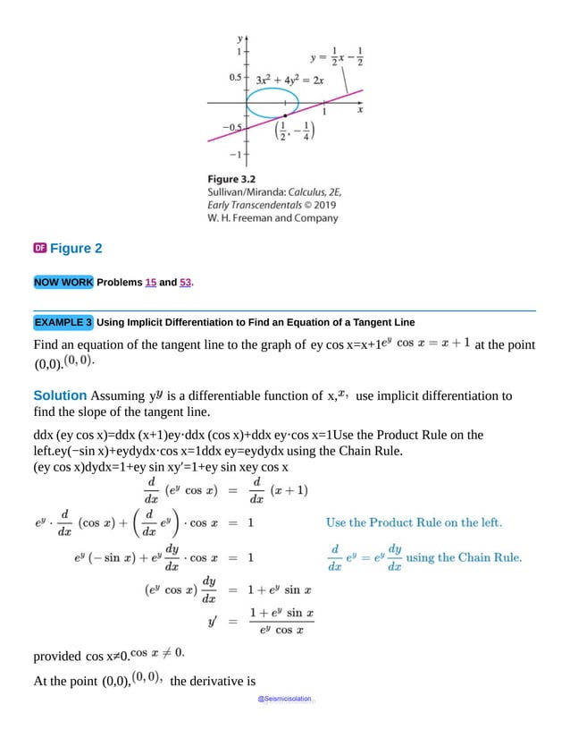
631. ddx [u(x)]r=r[u(x)]r−1u′(x)
provided ur and ur−1 are defined.
EXAMPLE 7 Differentiating Functions Using the Power Rule
a. dds (s3−2s+1)5⁄3=53 (s3−2s+1)2⁄3dds (s3−2s+1)=53 (s3−2s+1)2⁄3(3s2−2)
b. ddxx4−3x+53=ddx (x4−3x+5)1⁄3=13 (x4−3x+5)−2⁄3ddx (x4−3x+5)=4x3−33(x4−3x+5)2
c. ddθ[tan (3θ)]−3⁄4=−34[tan (3θ)]−7⁄4ddθ tan (3θ)=−34[tan (3θ)]−7⁄4⋅sec2 (3θ)⋅3=
−9 sec2 (3θ)4[tan (3θ)]7⁄4
▪
NOW WORK Problem 39.
3.2 Assess Your Understanding
Concepts and Vocabulary
1. True or False Implicit differentiation is a technique for finding the derivative of an
implicitly defined function.
2. True or False If yq=xp for integers p and q, then qyq−1=pxp−1.
3. ddx (3x1⁄3)=__________.
@Seismicisolation
@Seismicisolation

632. 4. If y=(x2+1)3⁄2, then y′=__________.
Skill Building
In Problems 5–30, find y′=dydx using implicit differentiation.
5. 3x+2y=3
6. 2x−5y=7
7. x2+y2=4
8. y4−4x2=4
9. ey=sin x
10. ey=tan x
11. ex+y=y
12. ex+y=x2
13. x2y=5
14. x3y=8
15. x2−y2−xy=2
16. x2−4xy+y2=y
17. 1x+1y=1
18. 1x−1y=4
19. x2+y2=2yx
20. x2+y2=2y2x2
21. ex sin y+ey cos x=4
22. ey cos x+e−x sin y=10
23. (x2+y)3=y
@Seismicisolation
@Seismicisolation

633. 24. (x+y2)3=3x
25. y=tan (x−y)
26. y=cos (x+y)
27. y=x sin y
28. y=x cos y
29. x2y=exy
30. yex=y−x
In Problems 31–46, find y′.
31. y=x2⁄3+4
32. y=x1⁄3−1
33. y=x23
34. y=x54
35. y=x3−1x3
36. y=x+1x
37. y=(x3−1)1⁄2
38. y=(x2−1)1⁄3
39. y=xx2−1
40. y=xx3+1
41. y=ex2−9
42. y=ex
43. y=(x2 cos x)3⁄2
44. y=(x2 sin x)3⁄2
@Seismicisolation
@Seismicisolation

634. 45. y=(x2−3)3⁄2(6x+1)5⁄3
46. y=(2x3−1)4⁄3(3x+4)5⁄2
In Problems 47–52, find y′ and y″.
47. x2+y2=4
48. x2−y2=1
49. x2−y2=4+5x
50. 4xy=x2+y2
51. y=x2+1
52. y=4−x2
In Problems 53–58, for each implicitly defined equation:
a. Find the slope of the tangent line to the graph of the equation at the indicated point.
b. Write an equation for this tangent line.
c. Graph the tangent line on the same axes as the graph of the equation.
53. x2+y2=5 at (1,2)
54. (x−3)2+(y+4)2=25 at (0,0)
@Seismicisolation
@Seismicisolation

635. 55. x2−y2=8 at (3,1)
56. y2−3x2=6 at (1,−3)
@Seismicisolation
@Seismicisolation

636. 57. x24+y23=1 at −1,32
58. x2+y24=1 at 12,3
59. Find y′ and y″ at the point (−1,1) on the graph of
3x2y+2y3=5x2
60. Find y′ and y″ at the point (0,0) on the graph of
4x3+2y3=x+y
Applications and Extensions
In Problems 61–68, find y′.
(Hint: Use the fact that | x|=x2.)
@Seismicisolation
@Seismicisolation

637. 61. y=|3x |
62. y=|x5 |
63. y=|2x−1|
64. y=|5−x2 |
65. y=|cos x |
66. y=|sin x |
67. y=sin|x |
68. | x|+|y|=1
69. Tangent Line to a Hypocycloid The graph of
x2⁄3+y2⁄3=5
is called a hypocycloid. Part of its graph isshown in the figure. Find an equation of the
tangent line to the hypocycloid at the point (1,8 ).
70. Tangent Line At what point does the graph of y=1x have a tangent line parallel
to the line x+16y=5 ? See the Figure.
@Seismicisolation
@Seismicisolation

638. 71. Tangent Line For the equation x+xy+2y2=6 :
a. Find an expression for the slope of the tangent line at any point (x,y) on the
graph.
b. Write an equation for the line tangent to the graph at the point (2,1).
c. Find the coordinates of any other point on this graph with slope equal to the slope
at (2,1).
d. Graph the equation and the tangent lines found in parts (b) and (c) on the same
screen.
72. Tangent Line to a Lemniscate The graph of
(x2+y2)2=x2−y2
called a lemniscate, is shown in the figure. There are exactly four points at which the
tangent line to the lemniscate is horizontal. Find them.
73. Rectilinear Motion An object of mass m moves in rectilinear motion so that at time
t>0 its position s from the origin and its velocity v=dsdt satisfy the
equation
mv2−v02=ks02−s2
where k is a positive constant and v0 and s0 are the initial velocity and position,
respectively, of the object. Show that if v>0, then
ma=−ks
where a=d2sdt2 is the acceleration of the object.
[Hint: Differentiate the expression mv2−v02=ks02−s2 with
@Seismicisolation
@Seismicisolation

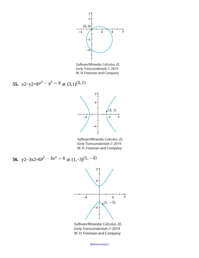
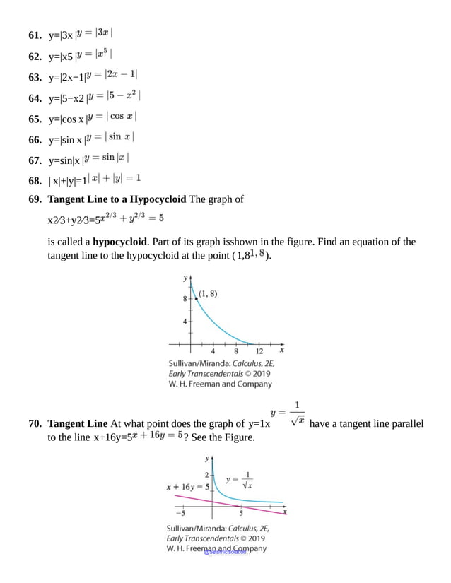
639. respect to t. ]
74. Price Function It is estimated that t months from now the average price (in dollars) of
a tablet will be given by
P(t)=3001+16t+100,0≤t≤60
a. Find P′(t)
b. Find P′(16) and P′(49) and interpret the results.
c. Graph P=P(t), and explain how the graph supports the answers in (b).
75. Production Function The production of commodities sometimes requires several
resources such as land, labor, and machinery. If there are two inputs that require
amounts x and y, then the output z is given by the function of two variables:
z=f(x,y). Here, z is called a production function. For example, if x
represents land, y represents capital, and z is the amount of a commodity produced, a
possible production function is z=x0.5y0.4. Set z equal to a fixed amount
produced and show that dydx=−5y4x. This illustrates that the rate of
change of capital with respect to land is always negative when the amount produced is
fixed.
76. Learning Curve The psychologist L. L. Thurstone suggested the following function for
the time T it takes to memorize a list of n words: T=f(n)=Cnn−b,
where C and b are constants depending on the person and
the task.
a. Find the rate of change of the time T with respect to the number n of words to
be memorized.
b. Suppose that for a certain person and a certain task, C=2 and b=2.
Find f′(10) and f′(30).
c. Interpret the results found in (c).
77. The Folium of Descartes The graph of the equation x3+y3=2xy is called
the folium of Descartes.
a. Find y′.
b. Find an equation of the tangent line to the folium of Descartes at the point (1,1).
@Seismicisolation
@Seismicisolation

640. c. Find any points on the graph where the tangent line to the graph is horizontal.
Ignore the origin.
d. Graph the equation x3+y3=2xy. Explain how the graph supports the
answers to (b) and (c).
78. If n is an even positive integer, show that the tangent line to the graph of y=xn
at (1,1) is perpendicular to the tangent line to the graph of y=xn at (−1,1).
79. At what point(s), if any, is the line y=x−1 parallel to the tangent line to the
graph of y=25−x2 ?
80. What is wrong with the following?
If x+y=ex+y, then 1+y′=ex+y(1+y′).
Since ex+y>0, then y′=−1 for all x. Therefore, x+y=ex+y
must be a line of slope −1.
81. Show that if a function y is differentiable, and x and y are related by the equation
xnym+xmyn=k, where k is a constant, then
dydx=−y(nxr+myr)x(mxr+nyr)wherer=n−m
82. Physics For ideal gases, Boyle’s law states that pressure is inversely proportional to
volume. A more realistic relationship between pressure P and volume V is given by
the van der Waals equation
P+aV2=CV−b
where C is the constant of proportionality, a is a constant that depends on molecular
attraction, and b is a constant that depends on the size of the molecules. Find dVdP,
which measures the compressibility of the gas.
83. Tangent Line Show that an equation for the tangent line at any point (x0,y0) on
the ellipse x2a2+y2b2=1 is xx0a2+yy0b2=1.
84. Tangent Line Show that the slope of the tangent line to a hypocycloid
x2⁄3+y2⁄3=a2⁄3, a>0, at any point for which x≠0, is
@Seismicisolation
@Seismicisolation

641. −y1⁄3x1⁄3.
85. Tangent Line Use implicit differentiation to show that the tangent line to a circle
x2+y2=R2 at any point P on the circle is perpendicular to OP,
where O is the center of the circle.
Challenge Problems
86. Let A=(2,1) and B=(5,2) be points on the graph of f(x)=x−1.
A line is moved upward on the graph so that it remains parallel to the
secant line AB. Find the coordinates of the last point on the graph of f before the
secant line loses contact with the graph.
Orthogonal Graphs Problems 87 and 88 require the following definition:
The graphs of two functions are said to be orthogonal if the tangent lines to the graphs are
perpendicular at each point of intersection.
87. a. Show that the graphs of xy=c1 and −x2+y2=c2 are orthogonal, where c1 and c2
are positive constants.
b. Graph each function on one coordinate system for c1=1,2,3 and
c2=1,9,25.
88. Find a>0 so that the parabolas y2=2ax+a2 and y2=a2−2ax
are orthogonal.
89. Show that if p and q>0 are integers, then y=xp⁄q is a differentiable
function of x.
90. We say that y is an algebraic function of x if it is a function that satisfies an
equation of the form
P0(x)yn+P1(x)yn−1+⋯+Pn−1(x)y+Pn(x)=0
where Pk(x), k=0,1,2,…,n, are polynomials. For example, y=x
satisfies
y2−x=0
Use implicit differentiation to obtain a formula for the derivative of an algebraic
function.
@Seismicisolation
@Seismicisolation

642. 1. = NOW WORK problem
= Graphing technology recommended
= Computer Algebra System recommended
* In Problem 89, you are asked to show that y=xp⁄q is differentiable.
@Seismicisolation
@Seismicisolation

643. 3.3 Derivatives of the Inverse Trigonometric Functions
OBJECTIVES When you finish this section, you should be able to:
1 Find the derivative of an inverse function
2 Find the derivative of the inverse trigonometric functions
The Chain Rule is used to find the derivative of an inverse function.
NEED TO REVIEW? Inverse functions are discussed in Section P.4, pp 37–40.
1 Find the Derivative of an Inverse Function
Suppose f is a function and g is its inverse function. Then
g(f(x))=x
for all x in the domain of f.
Then if both f and g are differentiable, we can differentiate both sides with respect to
x and use the Chain Rule.
ddx g(f(x))=ddx xg′(f(x))⋅f′(x)=1Use the Chain Rule on the left.
Since the product of the derivatives is never 0, each function has a nonzero derivative on
its domain.
Conversely, if a one-to-one function has a nonzero derivative, then its inverse function
also has a nonzero derivative as stated in the following theorem.
THEOREM Derivative of an Inverse Function
Let y=f(x) and x=g(y) be inverse functions. Suppose f is differentiable
on an open interval containing x0 and y0=f(x0). If f′(x0)≠0,
then g is differentiable at y0=f(x0) and
ddy g(y)y=y0=g′(y0)=1f′(x0)
(1)
@Seismicisolation
@Seismicisolation

644. where the notation ddy g(y)y=y0=g′(y0) means ddy g(y)
evaluated at y0.
We have three comments about this theorem, which is proved in Appendix B:
If y0=f(x0) and f′(x0)≠0 exists, then ddy g(y) exists at
y0.
Statement (1) can be used to find ddy g(y) at y0 without knowing a formula
for g=f−1, provided we can find x0 and f′(x0).
In Leibniz notation, statement (1) takes the form dydx=1dxdy.
IN WORDS The derivative of a function equals the reciprocal of the derivative of its inverse function.
EXAMPLE 1 Finding the Derivative of an Inverse Function
The function f(x)=x5+x has an inverse function g. Find g′(2).
Solution Using (1) with y0=2, we get
g′(2)=1f′(x0)where 2=f(x0)
To find x0, we use the equation
f(x0)=x05+x0=2
A solution is x0=1. So g′(2)=1f′(1). Since f′(x)=5x4+1,
then f′(1)=6≠0 and
g′(2)=1f′(1)=16
@Seismicisolation
@Seismicisolation

645. ▪
Observe in Example 1 that the derivative of the inverse function g at 2 was obtained
without actually knowing a formula for g.
NOW WORK Problem 5.
EXAMPLE 2 Finding an Equation of a Tangent Line
The function f(x)=x3+2x−4 is one-to-one and has an inverse function g.
Find an equation of the tangent line to the graph of g at the point (8,2) on g.
Solution The slope of the tangent line to the graph of g at the point (8,2) is g′(8).
Since f and g are inverses, g(8)=2 and f(2)=8. Now use (1) to
find g′(8).
g′(8)=1f′(2)g′(y0)=1f′(x0); x0=2; y0=8=114f′(x)=3x2+2; f′(2)=3⋅22+2=14
Now use the point-slope form of an equation of a line to find an equation of the tangent
line to g at (8,2).
y−2=114 (x−8)14y−28=x−814y−x=20
The line 14y−x=20 is tangent to the graph of g at the point (8,2 ). ▪
NOW WORK Problem 51.
2 Find the Derivative of the Inverse Trigonometric Functions
Table 1 lists the inverse trigonometric functions and their domains.
TABLE 1 The Domain of the Inverse Trigonometric Functions
f Restricted Domain f−1 Domain
@Seismicisolation
@Seismicisolation

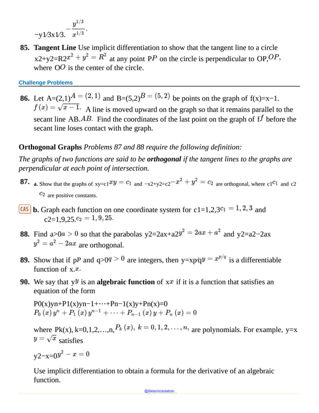
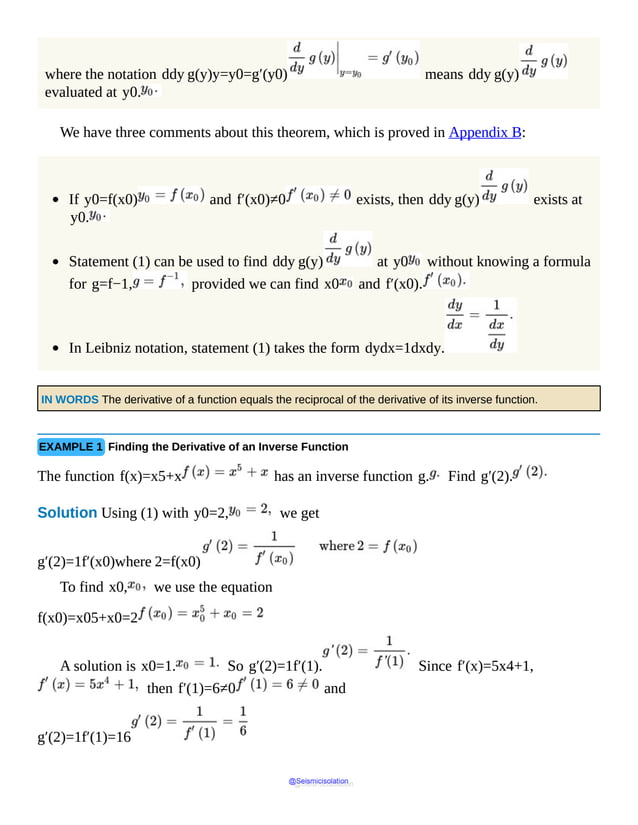
646. f(x)=sin x
−π2,π2
f−1(x)=sin−1 x
[−1,1]
f(x)=cos x [0,π] f−1(x)=cos−1 x [−1,1]
f(x)=tan x
−π2,π2 f−1(x)=tan−1 x (−∞,∞)
f(x)=csc x
−π,−π2∪0,π2 f−1(x)=csc−1 x | x|≥1
f(x)=sec x
0,π2∪π,3π2
f−1(x)=sec−1 x | x|≥1
f(x)=cot x (0,π) f−1(x)=cot−1 x (−∞,∞)
NEED TO REVIEW? Inverse trigonometric functions are discussed in Section P.7, pp. 61–64.
CAUTION Keep in mind that f−1(x) represents the inverse function of f and not the reciprocal
function. That is, f−1(x)≠1f(x).
To find the derivative of y=sin−1 x, −1≤x≤1, −π2≤y≤π2,
we write sin y=x and differentiate
implicitly with respect to x.
ddx sin y=ddx xcos y⋅dydx=1ddx sin y=cos y dydx using the Chain Rule.dydx=1cos y
provided cos y≠0. Since cos y=0 if y=−π2 or y=π2, we
exclude these values. Then ddx sin−1x=1cos y, −π2<y<π2.
Now, if −π2<y<π2, then cos y>0. Using a
Pythagorean identity, we have
@Seismicisolation
@Seismicisolation

647. NOTE Alternatively, we can use the Derivative of an Inverse Function. If y=sin−1 x, then x=sin y,
and
dydx=1dxdy=1cos y
provided cos y≠0.
THEOREM Derivative of y=sin−1 x
The derivative of the inverse sine function y=sin−1 x is
y′=ddx sin−1 x=11−x2−1<x<1
EXAMPLE 3 Using the Chain Rule with the Inverse Sine Function
Find y′ if:
a. y=sin−1(4x2)
b. y=esin−1 x
Solution a. If y=sin−1u and u=4x2, then dydu=11−u2
and dudx=8x. By the Chain Rule,
y′=dydx=dydu⋅dudx=11−u2(8x)=8x1−16x4u=4x2
b. If y=eu and u=sin−1x, then dydu=eu and dudx=11−x2.
By the Chain Rule,
@Seismicisolation
@Seismicisolation

648. ▪
NOW WORK Problem 27.
To derive a formula for the derivative of y=tan−1 x, −∞<x<∞, −π2<y<π2,
we write tan y=x and differentiate
implicitly with respect to x. Then
ddx tan y=ddx xsec2 y dydx=1Use the Chain Rule on the left.dydx=1sec2 y
Since −π2<y<π2, then sec y≠0.
Now use the Pythagorean identity sec2 y=1+tan2 y, and substitute
x=tan y. Then
y′=ddx tan−1 x=11+x2
THEOREM Derivative of y=tan−1 x
The derivative of the inverse tangent function y=tan−1 x is
y′=ddx tan−1 x=11+x2
The domain of y′ is all real numbers.
EXAMPLE 4 Using the Chain Rule with the Inverse Tangent Function
Find y′ if:
a. y=tan−1 (4x)
b. y=sin (tan−1 x)
@Seismicisolation
@Seismicisolation

649. Solution a. Let y=tan−1 u and u=4x. Then dydu=11+u2
and dudx=4. By the Chain Rule,
y′=dydx=dydu⋅dudx=11+u2⋅4=41+16x2
b. Let y=sin u and u=tan−1 x. Then dydu=cos u and
dudx=11+x2. By the Chain Rule,
y′=dydx=dydu⋅dudx=cos u⋅11+x2=cos (tan−1 x)1+x2
▪
NOW WORK Problem 35.
Finally to find the derivative of y=sec−1 x,| x|≥1, 0≤y<π2
or π≤y<3π2, we write x=sec y and use implicit differentiation.
ddx x=ddx sec y1=sec y tan y dydxUse the Chain Rule on the right.
We can solve for dydx provided sec y≠0 and tan y≠0, or equivalently,
y≠0 and y≠π. That is,
dydx=1sec y tan y,provided 0<y<π2 or π<y<3π2.
With these restrictions no y, tan y>0. * Now we use the Pythagorean identity
1+tan2 y=sec2 y. Then tan y=sec2 y−1 and
@Seismicisolation
@Seismicisolation

650. THEOREM Derivative of y=sec−1 x
The derivative of the inverse secant function y=sec−1 x is
y′=ddx sec−1 x=1xx2−1|x|>1
Notice that y=sec−1 x is not differentiable when x=±1. In fact, as
Figure 4 shows, at the points −1,π and (1,0), the graph of y=sec−1 x
has vertical tangent lines.
Figure 4 y=sec−1 x,|x|≥1, 0≤y<π2 or π≤y<3π2
Diagram
shows
a
piecewise
function
NOW WORK Problem 19.
The formulas for the derivatives of the three remaining inverse trigonometric functions
can be obtained using the following identities:
@Seismicisolation
@Seismicisolation

651. Since cos−1 x=π2−sin−1 x, then ddx cos−1 x=−11−x2,
where | x|<1.
Since cot−1 x=π2−tan−1 x, then ddx cot−1 x=−11+x2,
where −∞<x<∞.
Since csc−1 x=π2−sec−1 x, then ddx csc−1 x=−1xx2−1,
where | x|>1.
3.3 Assess Your Understanding
Concepts and Vocabulary
1. True or False If f is a one-to-one differentiable function and if f′(x)>0, then
f has an inverse function whose derivative is positive.
2. True or False ddx tan−1 x=11+x2, where −∞<x<∞.
3. True or False If f and g are inverse functions, then
g′(y0)=1f′(y0)
4. ddx sin−1 x= _____ where −1<x<1.
Skill Building
In Problems 5–8, the functions f and g are inverse functions.
5. If f(0)=4 and f′(0)=−2, find g′(4).
6. If f(1)=−2 and f′(1)=4, find g′(−2).
7. If g(3)=−2 and g′(3)=12, find f′(−2).
@Seismicisolation
@Seismicisolation

652. 8. If g(−1)=0 and g′(−1)=−13, find f′(0).
In Problems 9–16, f and g are inverse functions. For each function f, find g′(y0).
9. f(x)=x5; y0=32
10. f(x)=x3; y0=27
11. f(x)=x2+2,x≥0; y0=6
12. f(x)=x2−5,x≥0; y0=4
13. f(x)=x1⁄3; y0=2
14. f(x)=x2⁄5; y0=4
15. f(x)=3x4⁄3+1; y0=49
16. f(x)=x2⁄3+5; y0=6
In Problems 17–42, find the derivative of each function.
17. f(x)=sin−1(4x)
18. f(x)=sin−1(3x−2)
19. g(x)=sec−1(3x)
20. g(x)=cos−1(2x)
21. s(t)=tan −1t2
22. s(t)=sec−1 t3
23. f(x)=tan−1(1−2x2)
24. f(x)=sin−1(1−x2)
25. f(x)=sec−1(x2+2)
26. f(x)=cos−1x2
27. F(x)=sin−1 ex
@Seismicisolation
@Seismicisolation

653. 28. F(x)=tan−1ex
29. g(x)=tan−11x
30. g(x)=sec−1x
31. g(x)=x sin−1x
32. g(x)=x tan−1(x+1)
33. s(t)=t2sec−1t3
34. s(t)=t2sin−1t2
35. f(x)=tan−1(sin x)
36. f(x)=sin−1(cos x)
37. G(x)=sin (tan−1 x)
38. G(x)=cos (tan−1 x)
39. f(x)=etan−1(3x)
40. f(x)=esec−1x2
41. g(x)=sin−1x1−x2
42. g(x)=sec−1xx2−1
In Problems 43–46, use implicit differentiation to find dydx.
43. y2+sin−1 y=2x
44. xy+tan−1 y=3
45. 40 tan−1 y2−π x3y=2π
46. sec−1 y−xy=π3
47. The function f(x)=x3+2x has an inverse function g. Find g′(0)
@Seismicisolation
@Seismicisolation

654. and g′(3).
48. The function f(x)=2x3+x−3 has an inverse function g. Find g′(−3)
and g′(0).
Applications and Extensions
49. Tangent Line
a. Find an equation for the tangent line to the graph of y=sin−1 x2 at the
origin.
b. Use technology to graph y=sin−1 x2 and the tangent line found in (a).
50. Tangent Line
a. Find an equation for the tangent line to the graph of y=tan−1 x at x=1.
b. Use technology to graph y=tan−1 x and the tangent line found in (a).
51. Tangent Line The function f(x)=2x3−x, x≥1, is one-to-one and
has an inverse function g. Find an equation of the tangent line to the graph of g at
the point (14,2) on g.
52. Tangent Line The function f(x)=x5−3x is one-to-one and has an inverse
function g. Find an equation of the tangent line to the graph of g at the point (−2,1)
on g.
53. Normal Line The function f(x)=x+2x1⁄3 is one-to-one and has an
inverse function g. Find an equation of the normal line to the graph of g at the point
( 3,1 ) on g.
54. Normal Line The function f(x)=x4+x, x>0, is one-to-one and
has an inverse function g. Find an equation of the normal line to the graph of g at
the point (2,1) on g.
55. Rectilinear Motion An object moves along the x -axis so that its position x from the
origin (in meters) is given by x(t)=sin−11t, t>0, where t is the
time in seconds.
a. Find the velocity of the object at t=2 s.
b. Find the acceleration of the object at t=2 s.
@Seismicisolation
@Seismicisolation

655. 56. If g(x)=cos−1(cos x), show that g′(x)=sin x|sin x|.
57. Show that ddx tan−1(cot x)=−1.
58. Show that ddx cot−1x=ddx tan−11x for all x≠0.
59. Show that ddx sin−1 x−x1−x2=2x21−x2.
Challenge Problem
60. Another way of finding the derivative of y=xn is to use inverse functions. The
function y=f(x)=xn, n a positive integer, has the derivative f′(x)=nxn
−1. So, if x≠0, then f′(x)≠0. The inverse function of
f, namely, x=g(y)=yn, is defined for all y if n is odd and for all
y≥0 if n is even. Since this inverse function is differentiable for all y≠0,
we have
g′(y)=ddyyn=1f′(x)=1nxn−1
Since nxn−1=nynn−1=ny(n−1)⁄n=ny1−(1⁄n),
we have
ddyyn=ddy y1⁄n=1ny1−(1⁄n)=1n y(1⁄n)−1
Use the result from above and the Chain Rule to prove the formula
ddx xp⁄q=pq x(p⁄q)−1
1. = NOW WORK problem
= Graphing technology recommended
= Computer Algebra System recommended
* The restricted domain of f(θ)=sec θ was chosen as θ 0≤θ<π2 or π≤θ<3π2
@Seismicisolation
@Seismicisolation

656. so that tan θ≥0.
@Seismicisolation
@Seismicisolation

657. 3.4 Derivatives of Logarithmic Functions
OBJECTIVES When you finish this section, you should be able to:
1 Differentiate logarithmic functions
2 Use logarithmic differentiation
3 Express e as a limit
Recall that the function f(x)=ax, where a>0 and a≠1, is one-to-one
and is defined for all real numbers. We know from Section 3.1 that f′(x)=ax ln a
and that the domain of f′(x) is also the set of all real numbers.
Moreover, since f′(x)≠0, the inverse of f, y=logax, is differentiable on
its domain 0,∞. See Figure 5 for the graphs of y=ax and y=logax,
a>0, a≠1.
Figure 5
When
a
is
between
0
and
NEED TO REVIEW? Logarithmic functions are discussed in Section P.5, pp. 45–48.
1 Differentiate Logarithmic Functions
To find y′=ddxlogax, we use the fact that the following statements are
@Seismicisolation
@Seismicisolation

658. (1)
equivalent:
y=logaxifandonlyifx=ay
That is, y=logax and x=ay are inverse functions.
Using the Derivative of an Inverse Function and the fact that dxdy=ay ln a,
we have
THEOREM Derivative of a Logarithmic Function
The derivative of the logarithmic function y=logax, x>0, a>0, and
a≠1, is
y′=ddxlogax=1x ln ax>0
When a=e, then ln a=ln e=1, and (1) gives the formula for the
derivative of the natural logarithm function f(x)=ln x.
THEOREM Derivative of the Natural Logarithm Function
The derivative of the natural logarithm function y=ln x, x>0, is
y′=ddx ln x=1x
EXAMPLE 1 Differentiating Logarithmic Functions
Find y′ if:
a. y=(ln x)2
b. y=12logx
c. ln x+ln y=2x
d. y=log2x3
@Seismicisolation
@Seismicisolation

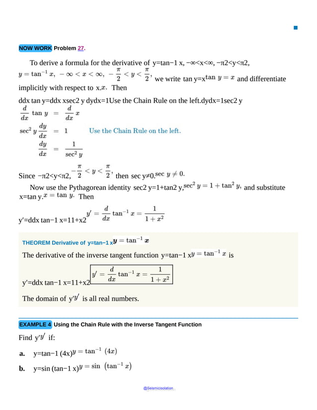
659. Solution a. We use the Power Rule for Functions. Then
b. Remember that logx=log10x. Then y=12logx=12log10x.
y′=12 ddxlog10x=12⋅1x ln10=12x ln10ddxlogax=1x ln a
c. We assume y is a differentiable function of x and use implicit differentiation. Then
ddx ln x+ln y=ddx (2x)ddx ln x+ddx ln y=21x+1y dydx=2ddx ln y= 1y dydxy
′=dydx= y 2−1x=y 2x−1xSolve for y′=dydx.
d. We use a property of logarithms and write
y=log2x3=3 log2 xlogaur=rlogau
Then,
y′=3 ddx log2 x=3 1x ln 2=3x ln 2
▪
NOW WORK Problem 9.
If y=ln[u(x)], where u=u(x)>0 is a differentiable function of
x, then by the Chain Rule,
dydx=dydu⋅dudx=1ududx=u′(x)u(x)
@Seismicisolation
@Seismicisolation

660. ddx ln[u(x)]=u′(x)u(x)
EXAMPLE 2 Differentiating Logarithmic Functions
Find y′ if:
a. y=ln(5x)
b. y=x ln(x2+1)
c. y=ln|x |
Solution
a.
y′=ddx ln(5x)=ddx (5x)5x=55x=1xddx ln u(x)=u′(x)u(x)
b.
c. Express y=|x | as a piecewise-defined function. Then
y=ln|x|=ln xifx>0ln(−x)ifx<0y′=ddx ln|x|=1xifx>01−x (−1)=1xifx<0
That is, ddx ln|x |=1x for all numbers x≠0. ▪
Another way to find the derivative of y=ln|x | is to express y as y=ln(x2)
@Seismicisolation
@Seismicisolation

661. and use the Chain Rule. See Problem 97.
Part (c) proves an important result that is used often:
ddx ln|x|=1xx≠0
Look at the graph of y=ln|x| (in blue) in Figure 6. As we move from left to right
along the graph, starting where x is unbounded in the negative direction and ending near
the y -axis, we see that the tangent lines to y=ln|x| go from being nearly horizontal
with negative slope to being nearly vertical with a very large negative slope. This is reflected
in the graph of the derivative y′=1x, where x<0 : The graph (in green) starts
close to zero and slightly negative and gets more negative as the y -axis is approached.
Figure 6
For
ln
of
modulus
of
x,
as
x
approaches
Similar remarks hold for x>0. The graph of y′=1x just to the right of the y
-axis is unbounded in the positive direction (the tangent lines to y=lnx are nearly
vertical with positive slope). As x becomes unbounded in the positive direction, the graph
of y′ gets closer to zero but remains positive (the tangent lines to y=ln|x| are
nearly horizontal with positive slope).
NOW WORK Problem 17.
Properties of logarithms can sometimes be used to simplify the work needed to find a
@Seismicisolation
@Seismicisolation

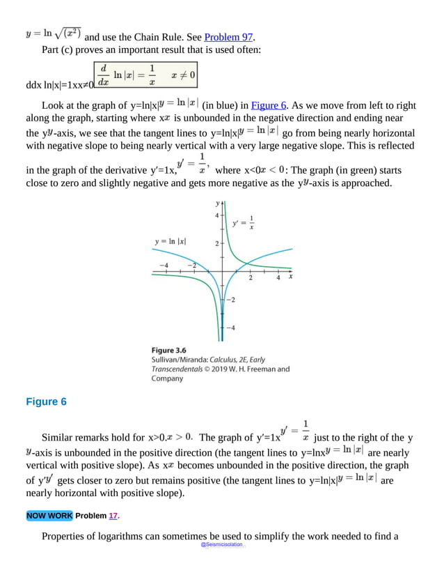
662. derivative.
NEED TO REVIEW? Properties of logarithms are discussed in Appendix A.1, pp. A-10 to A-11.
NOTE In the remaining examples, we do not explicitly state the domain of a function containing a logarithm.
Instead, we assume that the variable is restricted so all arguments for logarithmic functions are positive.
EXAMPLE 3 Differentiating Logarithmic Functions
Find y′ if y=ln2x−132x4+1x, x>12.
Solution Rather than attempting to use the Chain Rule, Quotient Rule, and Product Rule,
we first simplify the right side by using properties of logarithms.
y=ln(2x−1)32x4+1x=ln (2x−1)3+ln2x4+1−ln x=3ln(2x−1)+12 ln(2x4+1)−ln x
Now differentiate y.
y′=ddx 3 ln(2x−1)+12 ln(2x4+1)−ln x=ddx [3 ln(2x−1)]+ddx 12 ln(2x4+1)−ddx ln x=3⋅22x
−1+12⋅8x32x4+1−1x=62x−1+4x32x4+1−1x
▪
NOW WORK Problem 27.
2 Use Logarithmic Differentiation
Logarithms and their properties are very useful for finding derivatives of functions that
involve products, quotients, or powers. This method, called logarithmic differentiation,
uses the facts that the logarithm of a product is a sum, the logarithm of a quotient is a
@Seismicisolation
@Seismicisolation

663. difference, and the logarithm of a power is a product.
EXAMPLE 4 Finding Derivatives Using Logarithmic Differentiation
Find y′ if y=x25x+1(3x−2)3.
Solution It is easier to find y′ if we take the natural logarithm of each side before
differentiating. That is, we write
ln y=lnx25x+1(3x−2)3
and simplify using properties of logarithms.
ln y=ln[x25x+1]−ln (3x−2)3=ln x2+ln (5x+1)1⁄2− ln (3x−2)3=2 ln x+12 ln(5x+1)−3 ln(3x−2)
To find y′, use implicit differentiation.
ddx ln y=ddx 2 ln x+12 ln(5x+1)−3 ln(3x−2)y′y=ddx (2 ln x)+ddx 12 ln(5x+1)−ddx[3 ln(3x
−2)]ddx ln y=1ydydx=y′yy′y=2x+52(5x+1)−93x−2y′=y2x+52(5x+1)−93x−2=x25x+1(3x
−2)32x+52(5x+1)−93x−2
▪
@Seismicisolation
@Seismicisolation

664. ORIGINS Logarithmic differentiation was first used in 1697 by Johann Bernoulli (1667–1748) to find the
derivative of y=xx. Johann, a member of a famous family of mathematicians, was the younger brother
of Jakob Bernoulli (1654–1705). He was also a contemporary of Newton, Leibniz, the French mathematician
Guillaume de l’Hôhat; pital, and the Japanese mathematician Seki Takakazu (1642–1708).
Summarizing these steps, we have the method of Logarithmic Differentiation.
Steps for Using Logarithmic Differentiation
Step 1 If the function y=f(x) consists of products, quotients, and powers, take the
natural logarithm of each side. Then simplify using properties of logarithms.
Step 2 Differentiate implicitly, and use the fact that ddx ln y=y′y.
Step 3 Solve for y′, and replace y with f(x).
NOW WORK Problem 51.
EXAMPLE 5 Using Logarithmic Differentiation
Find y′ if y=xx, x>0.
Solution Notice that xx is neither x raised to a fixed power a, nor a fixed base a
raised to a variable power. We follow the steps for logarithmic differentiation:
Step 1 Take the natural logarithm of each side of y=xx, and simplify using
properties of logarithms.
ln y=ln xx=x ln x
Step 2 Differentiate implicitly.
ddx ln y=ddx (x ln x)y′y=x⋅ddx ln x+ddx x⋅ln x=x⋅1x+1⋅ln x=1+ln x
@Seismicisolation
@Seismicisolation

665. Step 3 Solve for y′=ddx xx : y′=y(1+ln x)=xx(1+ln x).
▪
Another way to find the derivative of y=xx uses the fact that y=xx=eln xx=ex ln x.
See Problem 85.
NOW WORK Problem 57.
EXAMPLE 6 Finding an Equation of a Tangent Line
Find an equation of the tangent line to the graph of f(x)=xx2+31+x at the
point (1,1).
Solution The slope of the tangent line to the graph of y=f(x) at the point (1,1)
is f′(1). Since the function consists of a product, a quotient, and a power, we
follow the steps for logarithmic differentiation:
Step 1 Take the natural logarithm of each side, and simplify:
ln y=ln xx2+31+x=ln x+12 ln(x2+3)−ln(1+x)
Step 2 Differentiate implicitly.
y′y=1x+12⋅2xx2+3−11+x=1x+xx2+3−11+x
Step 3 Solve for y′ and replace y with f(x) :
y′=f′(x)=y1x+xx2+3−11+x=xx2+31+x 1x+xx2+3−11+x
@Seismicisolation
@Seismicisolation

666. Now find the slope of the tangent line by evaluating f′(1).
f′(1)=42 1+14−12=34
Then an equation of the tangent line to the graph of f at the point (1,1) is
y−1=34 (x−1)y=34 x+14
▪
See Figure 7 for the graphs of f and y=34 x+14.
Figure 7
NOW WORK Problem 75.
We now can prove the Power Rule for finding the derivative of y=xa, where a
is any real number.
THEOREM Power Rule
If a is a real number, then
@Seismicisolation
@Seismicisolation

667. ddx xa=axa − 1
Proof Let y=xa, a real. Then ln y=ln xa=a ln x.
y′y=a 1xy′=ayx=axax=axa − 1
▪
EXAMPLE 7 Using the Power Rule
Find the derivative of:
a. y=x2
b. y=(x2+1)π
Solution a. We differentiate y using the Power Rule.
y′=ddx x2=2x2 − 1
b. The Power Rule for Functions also holds when the exponent is a real number. Then
y′=ddx (x2+1)π=π(x2+1)π − 1(2x)=2πx(x2+1)π − 1
▪
3 Express e as a Limit
In Section P.5, we stated that the number e has this property: ln e=1. Here we give
two equivalent ways of writing e as a limit; both are used in later chapters.
THEOREM The Number e as a Limit
The number e can be expressed by either of the two limits:
@Seismicisolation
@Seismicisolation

668. (a)limh→0(1+h)1⁄h=e(b)limn→∞1+1nn=e
(2)
Proof a. The derivative of f(x)=ln x is f′(x)=1x so f′(1)=1.
Then
Since y=ln x is continuous and f′(1)=1,
limh→0ln (1+h)1⁄h=lnlimh→0(1+h)1⁄h=1
Since ln e=1,
lnlimh→0(1+h)1⁄h=ln e
Since y=ln x is a one-to-one function,
limh→0(1+h)1⁄h=e
b. The limit above is true when h→0+. So if we let n=1h, then as h→0+,
we have n=1h→∞ and
e=limn→∞1+1nn
▪
Table 2 shows the values of 1+1nn for selected values of n.
TABLE 2
@Seismicisolation
@Seismicisolation

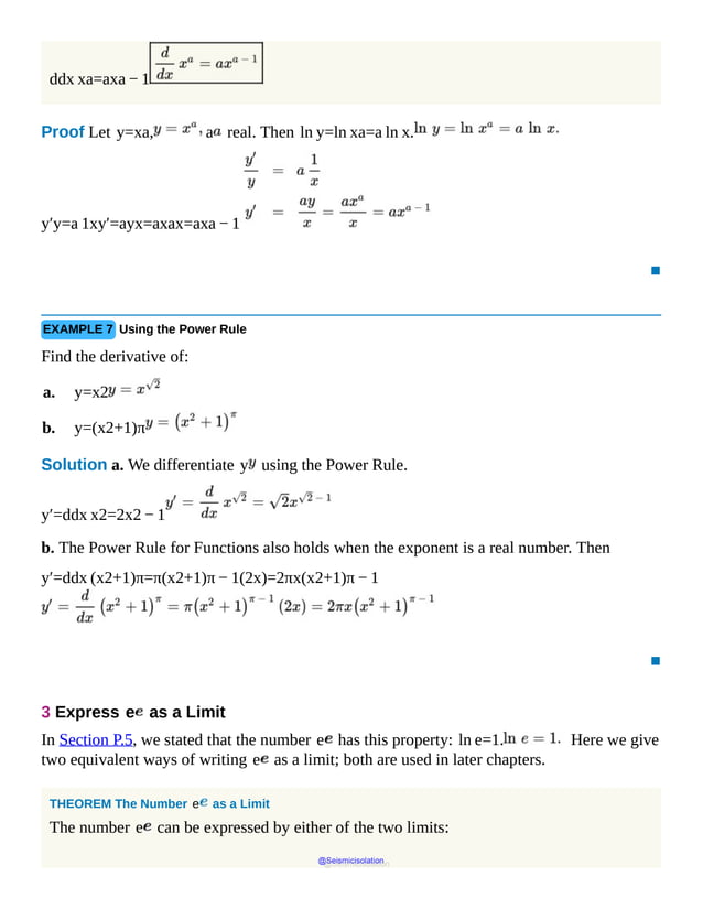
669. n
1+1nn
10 2.59374246
1000 2.716923932
10,000 2.718145927
106 2.718280469
NOTE Correct to nine decimal places,
e=2.718 281828
EXAMPLE 8 Expressing a Limit in Terms of e
Express each limit in terms of the number e :
a. limh→0(1+2h)1⁄h
b. limn→∞1+3n2n
Solution a. limh→0(1+2h)1⁄h resembles limh→0(1+h)1⁄h,
and with some manipulation, it can be expressed in terms of limh→0(1+h)1⁄h.
(1+2h)1⁄h=[(1+2h)1⁄(2h)]2
Now let k=2h, and note that h→0 is equivalent to 2h=k→0. So,
b. limn→∞1+3n2n resembles limn→∞1+1nn. We rewrite it
as follows:
1+3n2n=1+3n2n3⁄3=1+3nn⁄36
Let k=n3. Since n→∞ is equivalent to n3=k→∞, we find that
@Seismicisolation
@Seismicisolation

670. limn→∞1+3n2n=limk→∞ 1+1kk6=limk→∞ 1+1kk6=e6
▪
NOW WORK Problem 77.
The number e occurs in many applications. For example, in finance, the number e is
used to find continuously compounded interest. See the discussion preceding Problem 89.
3.4 Assess Your Understanding
Concepts and Vocabulary
1. ddx ln x=_______________.
2. True or False ddx xe=e xe−1.
3. True or False ddx ln[x sin2 x]=ddx ln x⋅ddx ln sin2 x.
4. True or False ddx ln π=1π.
5. ddx ln|x|= __________ for all x≠0.
6. limn→∞1+1nn=_______________.
Skill Building
In Problems 7–44, find the derivative of each function.
7. f(x)=5 ln x
8. f(x)=−3 ln x
9. s(t)=log2 t @Seismicisolation
@Seismicisolation

671. 10. s(t)=log3t
11. g(x)=(cos x)(ln x)
12. g(x)=(sin x)(ln x)
13. F(x)=ln(3x)
14. F(x)=ln x2
15. s(t)=ln(et−e−t)
16. s(t)=ln(e3t+e−3t)
17. f(x)=x ln(x2+4)
18. f(x)=x ln(x2+5x+1)
19. f(x)=x2log5(3x+5)
20. f(x)=x3log4(2x+3)
21. f(x)=12 ln 1+x1−x
22. f(x)=12 ln 1+x21−x2
23. f(x)=ln(ln x)
24. f(x)=lnln 1x
25. g(x)=ln xx2+1
26. g(x)=ln 4x3x2+4
27. f(x)=ln (x2+1)2xx2−1
28. f(x)=ln x3x−1(x2+1)3
29. F(θ)=ln(sin θ) @Seismicisolation
@Seismicisolation

672. 30. F(θ)=ln(cos θ)
31. g(x)=lnx+x2+4
32. g(x)=lnx+1+x
33. f(x)=log2(1+x2)
34. f(x)=log2(x2−1)
35. f(x)=tan−1(ln x)
36. f(x)=sin−1(ln x)
37. s(t)=ln(tan−1 t)
38. s(t)=ln(sin−1 t)
39. G(x)=(ln x)1⁄2
40. G(x)=(ln x)−1⁄2
41. f(θ)=sin (ln θ)
42. f(θ)= cos (ln θ)
43. g(x)=(log3 x)3⁄2
44. g(x)=(log2 x)4⁄3
In Problems 45–50, use implicit differentiation to find y′=dydx.
45. x ln y+y ln x=2
46. ln yx+ln xy=2
47. ln(x2+y2)=x+y
48. ln(x2−y2)=x−y
49. ln yx=y
50. ln yx−ln xy=1 @Seismicisolation
@Seismicisolation

673. In Problems 51–72, use logarithmic differentiation to find y′ . Assume that the variable is
restricted so that all arguments of logarithm functions are positive.
51. y=(x2+1)2(2x3−1)4
52. y=(3x2+4)3(x2+1)4
53. y=x2(x3+1)x2+1
54. y=x(x3+2)23x+43
55. y=x cos x(x2+1)3sin x
56. y=x sin x(1+ex)3cos x
57. y=(3x)x
58. y=(x−1)x
59. y=xln x
60. y=(2x)ln x
61. y=xx2
62. y=(3x)x
63. y=xex
64. y=(x2+1)ex
65. y=xsin x
66. y=xcos x
67. y=(sin x)x
68. y=(cos x)x
69. y=(sin x)cos x
@Seismicisolation
@Seismicisolation

674. 70. y=(sin x)tan x
71. xy=4
72. yx=10
In Problems 73–76, find an equation of the tangent line to the graph of y=f(x) at the
given point.
73. y=ln(5x) at 15,0
74. y=x ln x at (1,0)
75. y=x23x−2(x−1)2 at (2,8)
76. y=x(x3+1)2x+1 at (8,24)
In Problems 77–80, express each limit in terms of e.
77. limn→∞1+1n2n
78. limn→∞1+1nn⁄2
79. limn→∞1+13nn
80. limn→∞1+4nn
Applications and Extensions
81. Find d10dx10 (x9 ln x).
82. If f(x)=ln(x−1), find f(n)(x).
83. If y=ln(x2+y2), find the value of dydx at the point (1,0).
@Seismicisolation
@Seismicisolation

675. 84. If f(x)=tanln x−1ln x, find f′(e).
85. Find y′ if y=xx, x>0, by using y=xx=eln xx and the
Chain Rule.
86. If y=ln(kx), where x>0 and k>0 is a constant, show that y′=1x.
In Problems 87 and 88, find y′ . Assume that a is a constant.
87. y=x tan−1 xa−12 a ln(x2+a2),a≠0
88. y=x sin−1 xa+a lna2−x2,|a|>|x|,a≠0
Continuously Compounded Interest In Problems 89 and 90, use the following
discussion:
Suppose an initial investment, called the principal P, earns an annual rate of interest
r, which is compounded n times per year. The interest earned on the principal P
in the first compounding period is Prn, and the resulting amount A of the
investment after one compounding period is A=P+Prn=P1+rn.
After k compounding periods, the amount A of the
investment is A=P1+rnk. Since in t years there are nt
compounding periods, the amount A after t years is
A=P1+rnnt
When interest is compounded so that after t years the accumulated amount is A=
limn→∞P1+rnnt , the interest is said to be compounded continuously .
89. a. Show that if the annual rate of interest r is compounded continuously, then the
amount A after t years is A=Pert, where P is the initial investment.
b. If an initial investment of P =$5000 earns 2% interest compounded
continuously, how much is the investment worth after 10 years?
c. How long does it take an investment of $10,000 to double if it is invested at
@Seismicisolation
@Seismicisolation

676. 2.4% compounded continuously?
d. Show that the rate of change of A with respect to t when the interest rate r is
compounded continuously is dAdt=rA.
90. A bank offers a certificate of deposit (CD) that matures in 10 years with a rate of
interest of 3% compounded continuously. (See Problem 89.) Suppose you purchase
such a CD for $2000 in your IRA.
a. Write an equation that gives the amount A in the CD as a function of time t in
years.
b. How much is the CD worth at maturity?
c. What is the rate of change of the amount A at t=3? At t=5? At t=8?
d. Explain the results found in (c).
91. Sound Level of a Leaf Blower The loudness L, measured in decibels (dB), of a
sound of intensity I is defined as L(x)=10logI(x)I0, where x is
the distance in meters from the source of the sound and I0=10−12 W/m2
is the least intense sound that a human ear can detect. The intensity I
is defined as the power P of the sound wave divided by the area A on which it falls.
If the wave spreads out uniformly in all directions, that is, if it is spherical, the surface
area is A(x)=4πx2m2, and I(x)=P4πx2 W/m 2.
a. If you are 2.0 m from a noisy leaf blower and are walking away from it, at what rate
is the loudness L changing with respect to distance x ?
b. Interpret the sign of your answer.
92. Show that ln x+ln y=2x is equivalent to xy=e2x. Use this
equation to find y′. Compare this result to the solution found in Example 1(c).
93. If ln T=kt, where k is a constant, show that dTdt=kT.
94. Graph y=1+1xx and y=e on the same set of axes. Explain how the
graph supports the fact that limn→∞1+1nn=e.
95. Power Rule for Functions Show that if u is a function of x that is differentiable and
a is a real number, then
@Seismicisolation
@Seismicisolation

677. ddx [u(x)]a=a[u(x)]a−1u′(x)
provided ua and ua−1 are defined.
[Hint: Let |y|=|[u(x)]a| and use logarithmic differentiation.]
96. Show that the tangent lines to the graphs of the family of parabolas f(x)=−12 x2+k
are always perpendicular to the tangent lines to the graphs of the
family of natural logarithms g(x)=ln(bx)+c, where b>0, k,
and c are constants.
Source: Mathematics students at Millikin University, Decatur, Illinois.
97. Find the derivative of y=ln|x | by writing y=lnx2 and using the
Chain Rule.
Challenge Problem
98. If f and g are differentiable functions, and if f(x)>0, show that
ddx f(x)g(x)=g(x)f(x)g(x)−1f′(x)+f(x)g(x)[ln f(x)]g′(x)
1. = NOW WORK problem
= Graphing technology recommended
= Computer Algebra System recommended
@Seismicisolation
@Seismicisolation

678. 3.5 Differentials; Linear Approximations; Newton’s
Method
OBJECTIVES When you finish this section, you should be able to:
1 Find the differential of a function and interpret it geometrically
2 Find the linear approximation to a function
3 Use differentials in applications
4 Use Newton’s Method to approximate a real zero of a function
1 Find the Differential of a Function and Interpret It Geometrically
Recall that for a differentiable function y=f(x), the derivative can be defined as
dydx=f′(x)=limΔx→0 ΔyΔx=limΔx→0 f(x+Δx)−f(x)Δx
That is, for Δx sufficiently close to 0, we can make ΔyΔx as close as we please to
f′(x). This can be expressed as
ΔyΔx≈f′(x)whenΔx≈0Δx≠0
Then since Δx≠0,
Δy≈f′(x)ΔxwhenΔx≈0Δx≠0
(1)
DEFINITION Differential
Let y=f(x) be a differentiable function and let Δx denote a change in x.
The differential of x, denoted dx, is defined as dx=Δx≠0.
The differential of y, denoted dy, is defined as
dy=f′(x)dx
(2)
@Seismicisolation
@Seismicisolation

679. From statement (1), if Δx≈0, then Δy≈dy=f′(x)dx. That is,
when the change Δx in x is close to 0, then the differential dy is an approximation
to the change Δy in y.
To see the geometric relationship between Δy and dy, we use Figure 8. There, P=
(x,y) is a point on the graph of y=f(x) and Q=(x+Δx,y+Δy)
is a nearby point also on the graph of f. The change Δy in y
Δy=f(x+Δx)−f(x)
is the distance from M to Q. The slope of the tangent line to the graph of f at P is f
′(x)=dydx. So numerically, the differential dy measures the distance from M
to N. For Δx close to 0, dy=f′(x)dx will be close to Δy.
Figure 8
It
shows
a
steadily
rising
curve
depicting
function
f
of
IN WORDS
Δy equals the change in height of the graph of f from x to x+Δx ;
dy equals the change in height of the tangent line to the graph of f from x to
x+Δx.
EXAMPLE 1 Finding and Interpreting Differentials Geometrically
For the function f(x)=xex : @Seismicisolation
@Seismicisolation

680. a. Find an equation of the tangent line to the graph of f at (0,0).
b. Find the differential dy.
c. Compare dy to Δy when x=0 and Δx=0.5.
d. Compare dy to Δy when x=0 and Δx=0.1.
e. Compare dy to Δy when x=0 and Δx=0.01.
f. Interpret the results.
Solution a. The slope of the tangent line is
f′(x)=xex+exUse the Product Rule.
At (0,0), f′(0)=1, so an equation of the tangent line to the graph of f at
(0,0) is y=x.
b. dy=f′(x)dx=(xex+ex)dx=(x+1)exdx.
c. See Figure 9(a). When x=0 and Δx=dx=0.5, then
dy=(x+1)exdx=(0+1)e0(0.5)=0.5
The tangent line y=x rises by 0.5 as x changes from 0 to 0.5. The
corresponding change in the height of the graph f is
Δy=f(x+Δx)−f(x)=f(0.5)−f(0)=0.5e0.5−0≈0.824|Δy−dy|≈|0.824−0.5|=0.324
The graph of the tangent line is approximately 0.324 below the graph of f at
x=0.5.
Figure 9
@Seismicisolation
@Seismicisolation

681. d. See Figure 9(b). When x=0 and Δx=dx=0.1, then
dy=(0+1)e0(0.1)=0.1
The tangent line y=x rises by 0.1 as x changes from 0 to 0.1. The
corresponding change in the height of the graph f is
Δy=f(x+Δx)−f(x)=f(0.1)−f(0)=0.1 e0.1−0≈0.111|Δy−dy|≈0.111−0.1=0.011
The graph of the tangent line is approximately 0.011 below the graph of f at x=0.1.
e. See Figure 9(c). When x=0 and Δx=dx=0.01, then
dy=(0+1)e0(0.01)=0.01
The tangent line y=x rises by 0.01 as x changes from 0 to 0.01. The
corresponding change in the height of the graph of f is
Δy=f(x+Δx)−f(x)=f(0.01)−f(0)=0.01 e0.01−0≈0.0101|Δy−dy|≈|0.0101−0.01|=0.0001
The graph of the tangent line is approximately 0.0001 below the graph of f at
x=0.01.
f. The closer Δx is to 0, the closer dy is to Δy. So, we conclude that the closer
Δx is to 0, the less the tangent line departs from the graph of the function. That is, we
can use the tangent line to f at a point P as a linear approximation to f near P.
▪
NOW WORK Problems 9 and 19.
Example 1 shows that when dx=Δx is close to 0, the tangent line can be used
as a linear approximation to the graph. We discuss next how to find this linear approximation.
2 Find the Linear Approximation to a Function
Suppose y=f(x) is a differentiable function and suppose (x0,y0) is a point on
the graph of f. Then
Δy=f(x)−f(x0)anddy=f′(x0)dx=f′(x0)Δx=f′(x0)(x−x0)
@Seismicisolation
@Seismicisolation

682. If dx=Δx is close to 0, then
Δy≈dyf(x)−f(x0)≈f′(x0)(x−x0)f(x)≈f(x0)+f′(x0)(x−x0)
See Figure 10. Each figure shows the graph of y=f(x) and the graph of the tangent
line at (x0,y0). The first two figures show the difference between Δy and dy.
The third figure illustrates that when Δx is close to 0,Δy≈dy.
Figure 10
THEOREM Linear Approximation
The linear approximation L(x) to a differentiable function f at x=x0 is
given by
L(x)=f(x0)+f′(x0)(x−x0)
(3)
The graph of the linear approximation y=L(x) is the tangent line to the graph of
f at x0. The closer x is to x0, the better the approximation. We call the line L a
local linear approximation of f near x0. Although L provides a good approximation
of f in an interval centered at x0, the next example shows that as the interval widens,
the accuracy of the approximation of L may decrease.
EXAMPLE 2 Finding the Linear Approximation to a Function
a. Find the linear approximation L(x) to f(x)=sin x near x=0.
@Seismicisolation
@Seismicisolation

683. b. Use L (x) to approximate sin −0.3, sin 0.1, sin 0.4,
sin 0.5, and sin π4.
c. Graph f and L.
Solution a. Note that f(0)=sin 0=0. Since f′(x)=cos x, then
f′(0)=cos 0=1. Then, the linear approximation L(x) to f at 0 is
L(x)=f (0)+f′(0) (x−0)=xUse Equation (3).
So, for x close to 0, the function f(x)=sin x can be approximated by the line
L(x)=x.
b. The approximate values of sin x using L(x)=x, the true values of sin x,
and the absolute error in using the approximation are given in Table 3. From Table 3,
we see that the farther x is from 0, the worse the line L(x)=x approximates
f(x)=sin x.
TABLE 3
L(x)=x f(x)=sin x
Error:
|x−sin x|
0.1 0.0998 0.0002
−0.3 −0.2955 0.0045
0.4 0.3894 0.0106
0.5 0.4794 0.0206
π4≈0.7854
0.7071 0.0783
c. See Figure 11 for the graphs of f(x)=sin x and L(x)=x.
@Seismicisolation
@Seismicisolation

684. Figure 11
▪
NOW WORK Problem 27.
The next two examples show applications of differentials. In these examples, we use the
differential to approximate the change.
3 Use Differentials in Applications
EXAMPLE 3 Measuring Metal Loss in a Mechanical Process
A spherical bearing has a radius of 3 cm when it is new. Use differentials to approximate the
volume of the metal lost after the bearing wears down to a radius of 2.971 cm. Find the actual
volume lost and compare the approximation to the actual volume lost.
@Seismicisolation
@Seismicisolation

685. Solution The volume V of a sphere of radius R is V=43 πR3. As a
machine operates, friction wears away part of the spherical bearing. The exact volume of
metal lost equals the change ΔV in the volume V of the sphere, when the change in the
radius of the bearing is ΔR=2.971−3=−0.029 cm. Since the change
ΔR is small, we use the differential dV to approximate the change ΔV. Then
The approximate loss in volume of the bearing is 3.28 cm3.
The actual loss in volume ΔV is
ΔV=V(R+ΔR)−V(R)=43 π⋅2.9713−43 π⋅33≈43 π(−0.7755)≈−3.248 cm3
The approximate change in volume overstates the actual change by 0.032 cm3.
▪
NOW WORK Problem 49.
The use of dy to approximate Δy when Δx=dx is small is also helpful in
approximating error. If Q is the quantity to be measured and if ΔQ is the change in Q,
then the
Relativeerroratx0inQ=|ΔQ|Q(x0)Percentageerroratx0inQ=|ΔQ|Q(x0)⋅100%
IN WORDS Relative error is the ratio of the change in a quantity to the original quantity.
For example, if Q=50 units and the change ΔQ in Q is measured to be 5
units, then
Relative error at 50inQ=550=0.10 Percentage error at 50inQ=10%
When Δx is small, dQ≈ΔQ. The relative error and percentage error at x0
in Q can be approximated by |dQ|Q(x0) and |dQ|Q(x0)⋅100%,
@Seismicisolation
@Seismicisolation

686. respectively.
EXAMPLE 4 Measuring Error in a Manufacturing Process
A company manufactures spherical ball bearings of radius 3 cm. The customer requires
a tolerance of no more than 1% in the radius.
a. Use differentials to approximate the relative error for the surface area.
b. Find the corresponding percentage error for the surface area.
c. Interpret the results in the context of the problem.
Solution a. The tolerance of no more than 1% in the radius R means that the relative
error in the radius R must be less than or equal to 0.01. That is, |ΔR|R≤0.01.
The surface area S of a sphere of radius R is given by the formula
S=4πR2. We seek the relative error in S,|ΔS|S, which can be
approximated by |dS|S.
The relative error in the surface area will be less than or equal to 0.02.
b. The corresponding percentage error for the surface area is
|ΔS|S⋅100%≈0.02⋅100%=2%
c. A tolerance of no more than 1% in the radius results in a possible percentage error of
2% in the surface area. The tolerance of 1% in the radius of the ball bearing means the
radius of the sphere must be somewhere between 3−0.01(3)=2.97 cm
and 3+0.01(3)=3.03 cm. The corresponding 2% error in the
surface area means the surface area lies within ±0.02 of S=4π R2=36π cm2.
That is, the surface area is between 35.28π≈110.84 cm2
and 36.72π≈115.36 cm2. A rather small error in
the radius results in a more significant variation in the surface area!
▪
NOW WORK Problem 61.
@Seismicisolation
@Seismicisolation

687. 4 Use Newton’s Method to Approximate a Real Zero of a Function
Newton’s Method is used to approximate a real zero of a function. Suppose a function y=f(x)
is defined on a closed interval [a,b], and its derivative f′ is continuous on
the interval (a,b). Also suppose that, from the Intermediate Value Theorem or from a
graph or by trial calculations, we know that the function f has a real zero in some open
subinterval of (a, b ).
Suppose c1 is some number in the subinterval of (a,b ). Draw the tangent line to the
graph of f at the point P1=(c1,f(c1)) and label as c2 the x -intercept of
the tangent line. See Figure 12. If c1 is a first approximation to the required zero of f,
then c2 is a second approximation to the zero. Repeated use of this procedure often
generates increasingly accurate approximations to the actual zero.
Figure 12
Suppose c1 has been chosen. We seek a formula for finding the approximation c2.
The coordinates of P1 are (c1,f(c1)), and the slope of the tangent line to the
graph of f at point P1 is f′(c1). So, the equation of the tangent line to graph of f
at P1 is
y−f(c1)=f′(c1)(x−c1)
To find the x -intercept c2, let y=0. Then c2 satisfies the equation
−f(c1)=f′(c1)(c2−c1)c2=c1−f(c1)f′(c1)iff′(c1)≠0Solveforc2.
@Seismicisolation
@Seismicisolation

688. Notice that we are using the linear approximation to f at the point (c1,f(c1)) to
approximate the zero.
Now repeat the process by drawing the tangent line to the graph of f at the point P2=
(c2,f(c2)) and label as c3 the x -intercept of the tangent line. By
continuing this process, we have Newton’s method.
Newton’s Method
Suppose a function f is defined on a closed interval [a,b] and its first derivative f′
is continuous and not equal to 0 on the open interval (a,b). If x=c1 is a
sufficiently close first approximation to a real zero of the function f in (a,b), then
the formula
c2=c1−f(c1)f′(c1)
gives a second approximation to the zero. The n th approximation to the zero is given by
cn=cn − 1−f(cn − 1)f′(cn − 1)
ORIGINS When Isaac Newton first introduced his method for finding real zeros in 1669, it was very different
from what we did here. Newton’s original method (also known as the Newton–Raphson Method) applied only
to polynomials, and it did not use calculus! In 1690 Joseph Raphson simplified the method and made it
recursive, again without calculus. It was not until 1740 that Thomas Simpson used calculus, giving the method
the form we use here.
The formula in Newton’s Method is a recursive formula, because each new
approximation is written in terms of the previous one. Since recursive processes are
particularly useful in computer programs, variations of Newton’s Method are used by many
computer algebra systems and graphing utilities to find the zeros of a function.
EXAMPLE 5 Using Newton’s Method to Approximate a Real Zero of a Function
Use Newton’s Method to find a fourth approximation to the positive real zero of the function
@Seismicisolation
@Seismicisolation

689. f(x)=x3+x2−x−2.
Solution Since f(1)=−1 and f(2)=8, we know from the Intermediate
Value Theorem that f has a zero in the interval (1,2). Also, since f is a polynomial
function, both f and f′ are differentiable functions. Now
f(x)=x3+x2−x−2andf′(x)=3x2+2x−1
We choose c1=1.5 as the first approximation and use Newton’s Method. The
second approximation to the zero is
c2=c1 − f(c1)f′(c1)=1.5− f(1.5)f′(1.5)=1.5− 2.1258.75≈1.2571429
Use Newton’s Method again, with c2=1.2571429. Then
f(1.2571429)≈0.3100644 and f′(1.2571429)≈6.2555106.
The third approximation to the zero is
c3=c2 − f (c2)f′ (c2)=1.2571429 − 0.31006416.2555102≈1.2075763
The fourth approximation to the zero is
c4=c3 − f (c3)f′ (c3)=1.2075763 − 0.01160125.7898745≈1.2055726
▪
Using graphing technology, the zero of f(x)=x3+x2 − x − 2 is
given as x=1.2055694. See Figure 13.
@Seismicisolation
@Seismicisolation

690. Figure 13 f(x)=x3+x2−x−2
NOW WORK Problem 35.
The table feature of a graphing calculator can be used to take advantage of the recursive
nature of Newton’s Method and speed up the computation.
EXAMPLE 6 Using Technology with Newton’s Method
The graph of the function f(x)=sin x+x2−1 is shown in Figure 14.
a. Use the Intermediate Value Theorem to confirm that f has a zero in the interval (0,1).
b. Use technology with Newton’s Method and a first approximation of c1=0.5 to
find a fourth approximation to the zero.
Figure 14 f(x)=sin x+x2−1
@Seismicisolation
@Seismicisolation

691. Solution a. The function f(x)=sin x+x2−1 is continuous on its
domain, all real numbers, so it is continuous on the closed interval [0,1]. Since f(0)=−1
and f(1)=sin 1≈0.841 have opposite signs, the Intermediate
Value Theorem guarantees that f has a zero in the interval (0,1).
b. We begin by finding f′(x)=cos x+2x. To use Newton’s Method with a
graphing calculator, enter
x−sin x+x2−1cos x+2xx−f(x)f′(x)
into the Y=editor, as shown in Figure 15. Then create a table (Figure 16) by
entering the initial value 0.5 in the X column. The graphing calculator computes
0.5−sin 0.5+0.52−1cos 0.5+2(0.5)=0.64410789
Figure 15
and displays 0.64411 in column Y1 next to 0.5. The value Y1 is the second
approximation c2 that we use in the next iteration. Now enter 0.64410789 in
the X column of the next row, and the new entry in column Y1 is the third
approximation c3. Repeat the process until the desired approximation is obtained. The
fourth approximation to the zero of f is 0.63673.
▪
@Seismicisolation
@Seismicisolation

692. Figure 16
NOW WORK Problem 43.
When Newton’s Method Fails
You may wonder, does Newton’s Method always work? The answer is no. The list below,
while not exhaustive, gives some conditions under which Newton’s Method fails.
Newton’s Method fails if the conditions of the theorem are not met
a. f′(cn)=0 : Algebraically, division by 0 is not defined. Geometrically, the
tangent line is parallel to the x -axis and so has no x -intercept.
b. f′(c) is undefined: The process cannot be used.
Newton’s Method fails if the initial estimate c1 is not “good enough:”
a. Choosing an initial estimate too far from the required zero could result in
approximating a different zero of the function.
b. The convergence could approach the zero so slowly that hundreds of iterations are
necessary.
Newton’s Method fails if the terms oscillate between two values and so never get closer
to the zero.
Problems 76–79 illustrate some of these possibilities.
3.5 Assess Your Understanding
Concepts and Vocabulary
1. Multiple Choice If y=f(x) is a differentiable function, the differential dy=
@Seismicisolation
@Seismicisolation

693. a. Δy
b. Δx
c. f(x)dx
d. f′(x)dx
2. A linear approximation to a differentiable function f near x0 is given by the
function L(x)=________.
3. True or False The difference |Δy−dy| measures the departure of the graph of
y=f(x) from the graph of the tangent line to f.
4. If Q is a quantity to be measured and ΔQ is the error made in measuring Q,
then the relative error in the measurement at x0 is given by the ratio _______.
5. True or False Newton’s Method uses tangent lines to the graph of f to approximate
the zeros of f.
6. True or False Before using Newton’s Method, we need a first approximation for the
zero.
Skill Building
In Problems 7–18, find the differential dy of each function.
7. y=x3−2x+1
8. y=ex+2x−1
9. y=4(x2+1)3⁄2
10. y=x2−1
11. y=3 sin (2x)+x
12. y=cos2(3x)−x
13. y=e−x
14. y=esin x
15. y=xex
16. y=e−xx
@Seismicisolation
@Seismicisolation

694. 17. y=sin−1(2x)
18. y=tan−1 x2
In Problems 19–24:
a. Find the differential dy for each function f.
b. Evaluate dy and Δy at the given value of x when (i) Δx=0.5 , (ii)
Δx=0.1 , and (iii) Δx=0.01.
c. Find the error |Δy−dy| for each choice of dx=Δx.
19. f(x)=ex at x=1
20. f(x)=e−x at x=1
21. f(x)=x2⁄3 at x=2
22. f(x)=x−1⁄2 at x=1
23. f(x)=cos x at x=π
24. f(x)=tan x at x=0
In Problems 25–32:
a. Find the linear approximation L(x) to f at x0.
b. Graph f and L on the same set of axes.
25. f(x)=(x+1)5,x0=2
26. f(x)=x3−1,x0=0
27. f(x)=x,x0=4
28. f(x)=x2⁄3,x0=1
29. f(x)=ln x,x0=1
30. f(x)=ex, x0=1
31. f(x)=cos x,x0=π3
32. f(x)=sin x,x0=π6
@Seismicisolation
@Seismicisolation

695. 33. Use differentials to approximate the change in:
a. y=f(x)=x2 as x changes from 3 to 3.001.
b. y=f(x)=1x+2 as x changes from 2 to 1.98.
34. Use differentials to approximate the change in:
a. y=x3 as x changes from 3 to 3.01.
b. y=1x−1 as x changes from 2 to 1.98.
In Problems 35–42, for each function:
a. Use the Intermediate Value Theorem to confirm that a zero exists in the given interval.
b. Use Newton’s Method with the first approximation c1 to find c3, the third
approximation to the real zero.
35. f(x)=x3+3x−5, interval: (1,2). Let c1=1.5.
36. f(x)=x3−4x+2, interval: (1,2). Let c1=1.5.
37. f(x)=2x3+3x2+4x−1, interval: (0,1). Let c1=0.5.
38. f(x)=x3−x2−2x+1, interval: (0,1). Let c1=0.5
39. f(x)=x3−6x−12, interval: (3,4). Let c1=3.5.
40. f(x)=3x3+5x−40, interval: (2,3). Let c1=2.5.
41. f(x)=x4−2x3+21x−23, interval: (1,2). Use a first
approximation c1 of your choice.
42. f(x)=x4−x3+x−2, interval: (1,2). Use a first
approximation c1 of your choice.
In Problems 43–48, for each function:
a. Use the Intermediate Value Theorem to confirm that a zero exists in the given interval.
b. Use technology with Newton’s Method to find c5, the fifth approximation to the real
zero. Use the midpoint of the interval for the first approximation c1.
43. f(x)=x+ex, interval: (−1,0)
44. f(x)=x−e−x, interval: (0,1)
@Seismicisolation
@Seismicisolation

696. 45. f(x)=x3+cos2 x, interval: (−1,0)
46. f(x)=x2+2 sin x−0.5, interval: (0,1)
47. f(x)=5−x2+2, interval: (4,5)
48. f(x)=2x2+x2⁄3−4, interval: (1,2)
Applications and Extensions
49. Area of a Disk A circular plate is heated and expands. If the radius of the plate
increases from R=10 cm to R=10.1 cm , use differentials to
approximate the increase in the area of the top surface.
50. Volume of a Cylinder In a wooden block 3 cm thick, an existing circular hole
with a radius of 2 cm is enlarged to a hole with a radius of 2.2 cm. Use
differentials to approximate the volume of wood that is removed.
51. Volume of a Balloon Use differentials toapproximate the change in volume of a
spherical balloon of radius 3 m as the balloon swells to a radius of 3.1 m.
52. Volume of a Paper Cup A manufacturer produces paper cups in the shape of a right
circular cone with a radius equal to one-fourth the height. Specifications call for the
cups to have a top diameter of 4 cm. After production, it is discovered that the
diameter measures only 3.8 cm. Use differentials to approximate the loss in
capacity of the cup.
53. Volume of a Sphere
a. Use differentials to approximate the volume of material needed to manufacture a
hollow sphere if its inner radius is 2 m and its outer radius is 2.1 m.
b. Is the approximation overestimating or underestimating the volume of material
needed?
c. Discuss the importance of knowing the answer to (b) if the manufacturer receives
an order for 10,000 spheres.
54. Distance Traveled A bee flies around a circle traced on an equator of a ball with a
radius of 7 cm at a constant distance of 2 cm from the ball. An ant travels
along the same circle but on the ball.
a. Use differentials to approximate how many more centimeters the bee travels than
the ant in one round-trip journey.
b. Does the linear approximation overestimate or underestimate the difference in the
distances the bugs travel? Explain.
55. Estimating Height To find the height of a building, the length of the shadow of a 3 -m
@Seismicisolation
@Seismicisolation

697. pole placed 9 m from the building is measured. See the Figure. This measurement is
found to be 1 m , with a percentage error of 1%.. The height of the building is
estimated to be 30 m. Use differentials to find the percentage error in the estimate.
56. Pendulum Length The period of the pendulum of a grandfather clock is T=2πlg,
where l is the length (in meters) of the pendulum, T is the period (in
seconds), and g is the acceleration due to gravity (9.8m/s2 ). Suppose an
increase in temperature increases the length l of the pendulum, a thin wire, by 1%.
What is the corresponding percentage error in the period? How much time will the clock
lose (or gain) each day?
57. Pendulum Length Refer to Problem 56. If the pendulum of a grandfather clock is
normally 1 m long and the length is increased by 10 cm , use differentials to
approximate the number of minutes the clock will lose (or gain) each day.
@Seismicisolation
@Seismicisolation

698. 58. Luminosity of the Sun The luminosity L of a star is the rate at which it radiates
energy. This rate depends on the temperature T (in kelvin where 0 K is absolute
zero) and the surface area A of the star’s photosphere (the gaseous surface that emits
the light). Luminosity at time t is given by the formula L(t)=σAT4,
where σ is a constant, known as the Stefan–Boltzmann constant.
As with most stars, the Sun’s temperature has gradually increased over the 5
billion years of its existence, causing its luminosity to slowly increase. For this problem,
we assume that increased luminosity L is due only to an increase in temperature T.
That is, we treat A as a constant.
a. Find the rate of change of the temperature T of the Sun with respect to time t.
Write the answer in terms of the rate of change of the Sun’s luminosity L with
respect to time t.
b. 4.5 billion years ago, the Sun’s luminosity was only 70% of what it is now.
If the rate of change of luminosity L with respect to time t is constant, then
ΔLΔt=0.3LcΔt=0.3Lc4.5, where Lc is the current
luminosity. Use differentials to approximate the current rate of change of the
temperature T of the Sun in degrees per century.
59. Climbing a Mountain Weight W is the force on an object due to the pull of gravity.
On Earth, this force is given by Newton’s Law of Universal Gravitation: W=GmMr2,
where m is the mass of the object, M=5.974×1024 kg
is the mass of Earth, r is the distance of the object from the center
of the Earth, and G=6.67×10−11 m3⁄(kg⋅s2) is the
universal gravitational constant. Suppose a person weighs 70 kg at sea level, that
is, when r=6370 km (the radius of Earth). Use differentials to approximate
the person’s change in weight at the top of Mount Everest, which is 8.8 km above
sea level. (In this problem we treat kilograms as weight.)
60. Body Mass Index The body mass index (BMI) is given by the formula
BMI=703 mh2
where m is the person’s weight in pounds and h is the person’s height in inches. A
BMI between 18.5 and 25 indicates that weight is normal, whereas a BMI
greater than 25 indicates that a person is overweight.
a. Suppose a man who is 5 ft 6 in. weighs 142 lb in the morning when he
first wakes up, but he weighs 148 lb in the afternoon. Calculate his BMI in
the morning and use differentials to approximate the change in his BMI in the
@Seismicisolation
@Seismicisolation

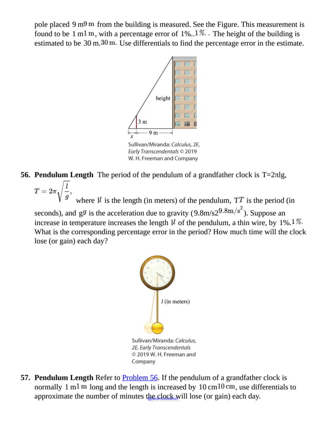
699. afternoon. Round both answers to three decimal places.
b. Did this linear approximation overestimate or underestimate the man’s afternoon
weight? Explain.
c. A woman who weighs 165 lb estimates her height at 68 in. with a possible
error of ±1.5 in. Calculate her BMI, assuming a height of 68 in. Then use
differentials to approximate the possible error in her calculation of BMI. Round the
answers to three decimal places.
d. In the situations described in (a) and (c), how do you explain the classification of
each person as normal or overweight?
61. Error Estimation The radius of a spherical ball is found by measuring the volume of
the sphere (by finding how much water it displaces). It is determined that the volume is
40 cubic centimeters (cm3 ), with a tolerance of no more than 1%.
a. Use differentials to approximate the relative error in measuring the radius.
b. Find the corresponding percentage error in measuring the radius.
c. Interpret the results in the context of the problem.
62. Error Estimation The oil pan of a car has the shape of a hemisphere with a radius of
8 cm. The depth h of the oil is measured at 3 cm , with a percentage error of
no more than 10%. [ Hint: The volume V for a spherical segment is V=13
πh2(3R−h), where R is the radius of the sphere.]
a. Use differentials to approximate the relative error in measuring the volume.
b. Find the corresponding percentage error in measuring volume.
c. Interpret the results in the context of the problem.
63. Error Estimation A closed container is filled with liquid. As the temperature T, in
degrees Celsius, increases, the pressure P, in atmospheres, exerted on the container
increases according to the ideal gas law, P=50 T.
a. If the relative error in measuring the temperature is no more than 0.01 , what is
the relative error in measuring the pressure?
b. Find the corresponding percentage error in measuring the pressure.
c. Interpret the results in the context of the problem.
64. Error Estimation A container filled with liquid is held at a constant pressure. As the
temperature T, in degrees Celsius, decreases, the volume V, in cm3, of the
container decreases according to the ideal gas law, V=15 T.
a. If the relative error in measuring the temperature is no more than 0.02 , what is
@Seismicisolation
@Seismicisolation

700. the relative error in measuring the volume?
b. Find the corresponding percentage error in measuring the volume.
c. Interpret the results in the context of the problem.
65. Percentage Error If the percentage error in measuring the edge of a cube is 2% ,
what is the percentage error in computing its volume?
66. Focal Length To photograph an object, a camera’s lens forms an image of the object on
the camera’s photo sensors. A camera lens can be approximated by a thin lens, which
obeys the thin-lens equation 1f=1p+1q, where p is the distance from the
lens to the object being photographed, q is the distance from the lens to the image of
the object, and f is the focal length of the lens. A camera whose lens has a focal length
of 50 mm is being used to photographa dog. The dog is originally 15 m
from the lens, but moves 0.33 m (about a foot) closer to the lens. Use differentials
to approximate the distance the image of the dog moved.
Using Newton’s Method to Solve Equations In Problems 67–70, use Newton’s Method to
solve each equation.
67. e−x=ln x
68. e−x=x−4
69. ex=x2
70. ex=2 cos x,x>0
71. Approximating e Use Newton’s Method to approximate the value of e by finding
the zero of the equation ln x−1=0. Use c1=3 as the first
approximation and find the fourth approximation to the zero. Compare the results from
this approximation to the value of e obtained with a calculator.
72. Show that the linear approximation of a function f(x)=(1+x)k, where x
is near 0 and k is any number, is given by y=1+kx.
73. Does it seem reasonable that if a first degree polynomial approximates a differentiable
function in an interval near x0, a higher-degree polynomial should approximate the
function over a wider interval? Explain your reasoning.
74. Why does a function need to be differentiable at x0 for a linear approximation to be
used?
75. Newton’s Method Suppose you use Newton’s Method to solve f(x)=0 for a
differentiable function f, and you obtain xn+1=xn. What can you
conclude?
@Seismicisolation
@Seismicisolation

701. 76. When Newton’s Method Fails Verify that the function f(x)=−x3+6x2−9x+6
has a zero in the interval (2,5). Show that Newton’s
Method fails if an initial estimate of c1=2.9 is chosen. Repeat Newton’s Method
with an initial estimate of c1=3.0. Explain what occurs for each of these two
choices. (The zero is near x=4.2. )
77. When Newton’s Method Fails Show that Newton’s Method fails for f(x)=x3−2x+2
with an initial estimate of c1=0.
78. When Newton’s Method Fails Show that Newton’s Method fails for f(x)=x8−1
if an initial estimate of c1=0.1 is chosen. Explain what occurs.
79. When Newton’s Method Fails Show that Newton’s Method fails for f(x)=(x−1)1⁄3
with an initial estimate of c1=2.
80. Newton’s Method
a. Use the Intermediate Value Theorem to show that f(x)=x4+2x3−2x−2
has a zero in the interval (−2,−1).
b. Use Newton’s Method to find c3, a third approximation to the zero from (a).
c. Explain why the initial approximation, c1=−1, cannot be used in (b).
81. Specific Gravity A solid wooden sphere of diameter d and specific gravity S sinks
in water to a depth h, which is determined by the equation 2x3−3x2−S=0,
where x=hd. Use Newton’s Method to find a third
approximation to h for a maple ball of diameter 6 in. for which S=0.786.
Use x=1.6 as the first approximation.
Challenge Problem
82. Kepler’s Equation The equation x−p sin x=M, called Kepler’s
equation, occurs in astronomy. Use Newton’s Method to find a second approximation to
x when p=0.2 and M=0.85. Use c1=1 as your first
approximation.
@Seismicisolation
@Seismicisolation

702. 3.6 Hyperbolic Functions
OBJECTIVES When you finish this section, you should be able to:
1 Define the hyperbolic functions
2 Establish identities for hyperbolic functions
3 Differentiate hyperbolic functions
4 Differentiate inverse hyperbolic functions
1 Define the Hyperbolic Functions
Functions involving certain combinations of ex and e−x occur so frequently in applied
mathematics that they warrant special study. These functions, called hyperbolic functions,
have properties similar to those of trigonometric functions. Because of this, they are named
the hyperbolic sine (sinh) , the hyperbolic cosine (cosh ), the hyperbolic tangent
(tanh ), the hyperbolic cotangent (coth ), the hyperbolic cosecant (csch ), and the
hyperbolic secant (sech ).
DEFINITION
The hyperbolic sine function and hyperbolic cosine function are defined as
y=sinh x=ex−e−x2 y=cosh x=ex+e−x2
Hyperbolic functions are related to a hyperbola in much the same way as the
trigonometric functions (sometimes called circular functions) are related to the circle. Just as
any point P on the unit circle x2+y2=1 has coordinates (cos t,sin t),
as shown in Figure 17, a point P on the hyperbola x2−y2=1 has
coordinates (cosht,sinh t), as shown in Figure 18. Moreover, both the sector
of the circle shown in Figure 17 and the shaded portion of Figure 18 have areas that each
equal t2.
@Seismicisolation
@Seismicisolation

703. Figure 17
Figure 18
The functions y=sinh x and y=cosh x are defined for all real
numbers. The hyperbolic sine function, y=sinh x, is an odd function, so its graph
is symmetric with respect to the origin; the hyperbolic cosine function, y=cosh x,
is an even function, so its graph is symmetric with respect to the y -axis. Their graphs may
be found by combining the graphs of y=ex2 and y=e−x2, as illustrated in
Figures 19 and 20, respectively. The range of y=sinh x is all real numbers, and the
range of y=cosh x is the interval [1,∞).
@Seismicisolation
@Seismicisolation

704. Figure 19 y=sinh x=ex − e−x2
Figure 20 y=cosh x=ex+e−x2
The remaining four hyperbolic functions are combinations of the hyperbolic cosine and
hyperbolic sine functions, and their relationships are similar to those of the trigonometric
functions.
Hyperbolic tangent:y=tanh x=sinh xcosh x=ex − e−xex+e−xHyperbolic
cotangent:y=coth x=cosh xsinh x=ex+e−xex−e−xHyperbolic secant:y=sech x=1cosh x=2ex+e
−xHyperbolic cosecant:y=csch x=1sinh x=2ex−e−x
@Seismicisolation
@Seismicisolation

705. The graphs of these four hyperbolic functions are shown in Figures 21 through 24.
Figure 21 y=tanh x
Figure 22 y=coth x
@Seismicisolation
@Seismicisolation

706. Figure 23 y=sech
Figure 24 y=csch x
EXAMPLE 1 Evaluating Hyperbolic Functions
Find the exact value of:
a. cosh 0
b. sech 0
c. tanh(ln 2)
Solution a. cosh 0=e0+e02=22=1
b. sech 0=1cosh 0=11=1
c. tanh(ln 2)=eln 2−e−ln 2eln 2+e−ln 2=2−eln(1⁄2)2+eln(1⁄2)=2−122+12=35
@Seismicisolation
@Seismicisolation

707. ▪
NOW WORK Problem 9.
The hyperbolic cosine function has an interesting physical interpretation. If a cable or
chain of uniform density is suspended at its ends, such as with high-voltage lines, it will
assume the shape of the graph of a hyperbolic cosine.
Suppose we fix our coordinate system, as in Figure 25, so that the cable, which is
suspended from endpoints of equal height, lies in the xy -plane, with the lowest point of
the cable at the point (0,b). Then the shape of the cable will be modeled by the
equation
y=a cosh xa+b−a
where a is a constant that depends on the weight per unit length of the cable and on the
tension or horizontal force holding the ends of the cable. The graph of this equation is called
a catenary, from the Latin word catena that means “chain.”
Figure 25 y=a cosh xa+b−a
2 Establish Identities for Hyperbolic Functions
There are identities for the hyperbolic functions that remind us of the trigonometric identities.
For example, tanh x=sinh xcosh x and coth x=1tanh x.
Other useful hyperbolic identities include
cosh2 x−sinh2 x=1tanh2 x+sech2 x=1coth2x−csch2 x=1
@Seismicisolation
@Seismicisolation

708. EXAMPLE 2 Establishing Identities for Hyperbolic Functions
Establish the identity cosh2 x−sinh2 x=1.
Solution
cosh2 x−sinh2 x=ex+e−x22 − ex−e−x22=e2x+2e0+e−2x4−e2x−2e0+e−2x4=2+24=1
▪
Below we list other identities involving hyperbolic functions that can be established.
Sum
formulas: sinh(A+B)=sinh A cosh B+cosh A sinh Bcosh(A+B)=cosh A cosh B+sinh
Even/odd
properties:sinh(−A)=−sinh Acosh(−A)=cosh A
The derivations of these identities are left as exercises. (See Problems 17–20.)
NOW WORK Problem 19.
3 Differentiate Hyperbolic Functions
Since the hyperbolic functions are algebraic combinations of ex and e−x, they are
differentiable at all real numbers for which they are defined. For example,
ddx sinh x=ddx ex−e−x2=12 ddx ex−ddx e−x=12 (ex+e−x) =cosh xddxcosh x=ddx ex+e
−x2=12 ddx ex+ddx e−x=12 (ex−e−x) =sinh xddxcsch x=ddx 1sinh x=−ddxsinh xsinh2 x=
−cosh xsinh2 x=−1sinh x⋅cosh xsinh x=−csch x coth x
@Seismicisolation
@Seismicisolation

709. The formulas for the derivatives of the hyperbolic functions are listed below.
ddx sinh x = ​coshxddx tanh x = sech2 xddx csch x=
−csch x coth xddx cosh x =sinhxddx coth x=−csch2xddx sech x=−sech x tanh x
EXAMPLE 3 Differentiating Hyperbolic Functions
Find y′.
a. y=x2−2 sinh x
b. y=cosh(x2+1)
Solution a. Use the Difference Rule.
y′=ddx (x2−2 sinh x)=ddx x2−2 ddx sinh x=2x−2 cosh x
b. Use the Chain Rule with y=cosh u and u=x2+1.
y′=dydx=dydu⋅dudx=sinh u⋅2x=2x sinh(x2+1)
▪
NOW WORK Problem 31.
EXAMPLE 4 Finding the Angle Between a Catenary and Its Support
@Seismicisolation
@Seismicisolation

710. A cable is suspended between two poles of the same height that are 20 m apart, as shown in
Figure 26(a). If the poles are placed at (−10,0) and (10,0), the equation that
models the height of the cable is y=10 coshx10+15. Find the angle θ
at which the cable meets a pole.
Solution The angle θ at which the cable meets the pole equals the angle between the
tangent line to the catenary at the point (10, 30.4) and the pole. The slope of the tangent line
to the cable is given by
y′=ddx 10 coshx10+15=10⋅110sinhx10=sinhx10
At x=10, the slope mtan of the tangent line is mtan=sinh1010=sinh 1.
To find the angle θ between the cable and the pole, we form a right triangle using the
tangent line and the pole, as shown in Figure 26(b).
Figure 26
From Figure 26(b), the slope of the tangent line is mtan=yx=sinh 1.
@Seismicisolation
@Seismicisolation

711. So tan θ=xy=1sinh 1 and θ=tan−11sinh 1≈0.7050
radians ≈40.4 ∘.
▪
NOW WORK Problem 61.
4 Differentiate Inverse Hyperbolic Functions
The graph of y=sinh x, shown in Figure 19 on p. 251, suggests that every
horizontal line intersects the graph at exactly one point. In fact, the function y=sinh x
is one-to-one, and so it has an inverse function. We denote the inverse by y=sinh
−1x and define it as
y=sinh−1xif and only ifx=sinhy
NEED TO REVIEW? One-to-one functions and inverse functions are discussed in Section P.4, pp. 35–40.
The domain of y=sinh−1 x is the set of real numbers, and the range is also
the set of real numbers. See Figure 27(a).
The graph of y=coshx (see Figure 20 on p. 251) shows that every horizontal
line above y=1 intersects the graph of y=coshx at two points so y=coshx
is not one-to-one. However, if the domain of y=coshx is restricted to the
nonnegative values of x, we have a one-to-one function that has an inverse. We denote the
inverse function by y=cosh−1 x and define it as
y=cosh−1xif and only ifx=coshy y≥0
The domain of y=cosh−1 x is x≥1, and the range is y≥0. See
Figure 27(b).
The other inverse hyperbolic functions are defined similarly. Their graphs are given in
Figure 27(c)–(f).
@Seismicisolation
@Seismicisolation

712. Figure 27
Inverse
of
sinh
x
is
an
s-
shaped
curve
lying
entirely
in
the
first
and
third
quadrants.
Inverse
of
cosh
x
is
a
Since the hyperbolic functions are defined in terms of the exponential function, the
inverse hyperbolic functions can be expressed in terms of natural logarithms.
y=sinh−1 x=ln x+x2+1 for all real x
y=cosh−1 x=ln x+x2−1 x≥1
y=tanh−1 x=12 ln1+x1−x |x|<1
y=coth−1 x=12 lnx+1x−1 |x|>1
We show that sinh−1x=ln x+x2+1 here, and leave the others as
exercises. (See Problems 71–73.)
EXAMPLE 5 Expressing the Inverse Hyperbolic Sine Function as a Natural Logarithm
Express y=sinh−1 x as a natural logarithm.
Solution Since y=sinh−1 x, where x=sinh y, we have
x=ey−e−y22xey=(ey)2−1Multiply both sides by 2ey.(ey)2−2xey−1=0
@Seismicisolation
@Seismicisolation

713. This is a quadratic equation in ey. Use the quadratic formula and solve for ey.
ey=2x±4x2+42=x±x2+1
NEED TO REVIEW? The quadratic formula is discussed in Appendix A.1, p. A-3.
Since ey>0 and x<x2+1 for all x, the minus sign on the right side
is not possible. As a result, ey=x+x2+1 so that
y=sinh−1 x=ln(x+x2+1)
▪
NOW WORK Problem 71.
EXAMPLE 6 Differentiating an Inverse Hyperbolic Sine Function
Show that if y=sinh−1x, then
y′=ddx sinh−1x=1x2+1.
Solution Since y=sinh−1 x=ln x+x2+1, we have
@Seismicisolation
@Seismicisolation

714. ▪
NOW WORK Problem 43.
Similarly, we have the following derivative formulas. If y=cosh−1 x, then
y′=ddx cosh−1 x=1x2−1x>1
If y=tanh−1 x, then
y′=ddx tanh−1 x=11−x2|x| <1
EXAMPLE 7 Differentiating an Inverse Hyperbolic Tangent Function
Find y′ if y=tanh−1x.
Solution Use the Chain Rule with y=tanh−1u and u=x. Then
▪
NOW WORK Problem 41.
3.6 Assess Your Understanding
Concepts and Vocabulary
1. True or Falsecsch x=1cosh x.
2. In terms of sinh x and cosh x, tanh x=______________.
3. True or False The domain of y=cosh x is [1,∞).
@Seismicisolation
@Seismicisolation

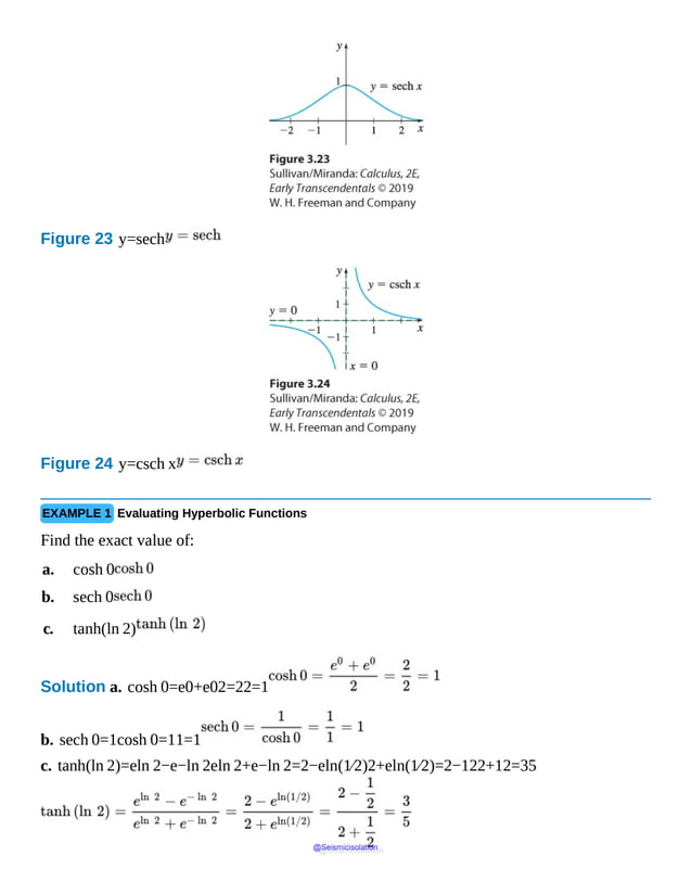
715. 4. Multiple Choice The function y=cosh x is [(a) even (b) odd (c) neither].
5. True or False cosh2 x+sinh2 x=1.
6. True or False ddxsinh x=1x2+1.
7. True or False The function y=sinh−1 x is defined for all real numbers x.
8. True or False The functions f(x)=tanh−1 x and g(x)=coth−1 x
are identical except for their domains.
Skill Building
In Problems 9–14, find the exact value of each expression.
9. csch(ln 3)
10. sech(ln 2)
11. cosh2(5)−sinh2(5)
12. cosh(−ln 2)
13. tanh 0
14. sinh ln 12
In Problems 15–24, establish each identity.
15. tanh2 x+sech2 x=1
16. coth2 x−csch2 x=1
17. sinh(−A)=−sinh A
18. cosh(−A)=cosh A
19. sinh(A+B)=sinh A cosh B+cosh A sinh B
20. cosh(A+B)=cosh A cosh B+sinh A sinh B
21. sinh(2x)=2 sinh x cosh x
@Seismicisolation
@Seismicisolation

716. 22. cosh(2x)=cosh2 x+sinh2 x
23. cosh(3x)=4 cosh3 x−3 cosh x
24. tanh(2x)=2 tanh x1+tanh2 x
In Problems 25–48, find the derivative of each function.
25. f(x)=sinh(3x)
26. f(x)=cosh x2
27. f(x)=cosh(x2+1)
28. f(x)=cosh(2x3−1)
29. g(x)=coth 1x
30. g(x)=tanh(x2)
31. F(x)=sinh x cosh(4x)
32. F(x)=sinh(2x) cosh(−x)
33. s(t)=cosh2 t
34. s(t)=tanh2 t
35. G(x)=ex cosh x
36. G(x)=ex(cosh x+sinh x)
37. f(x)=x2 sech x
38. f(x)=x3 tanh x
39. v(t)=cosh−1(4t)
40. v(t)=sinh−1(3t)
41. f(x)=tanh−1(x2−1)
42. f(x)=cosh−1(2x+1)
43. g(x)=x sinh−1 x
@Seismicisolation
@Seismicisolation

717. 44. g(x)=x2 cosh−1 x
45. s(t)=tanh−1(tan t)
46. s(t)=sinh−1(sin t)
47. f(x)=cosh−1 x2−1, x>2
48. f(x)=sinh−1 x2+1
In Problems 49–52, find y′.
49. sinh x+cosh y=x+y
50. sinh y−cosh x=x−y
51. ex cosh y=ln x
52. ey sinh x=ln y
In Problems 53–56, find y″.
53. y=(sinh x)2
54. y=(cosh x)3
55. y=cosh x3
56. y=sinh x2
In Problems 57–60, find an equation of the tangent line to the graph of f at the given point.
57. f(x)=sinh(2x) at (0,0)
58. f(x)=cosh x2 at (0,1)
59. f(x)=ex cosh x at (0,1)
60. f(x)=e−x sinh x at (0,0)
Applications and Extensions
61. Catenary A cable is suspended between two supports of the same height that are 100 m
apart. If the supports are placed at (−50,0) and (50,0), the equation that
models the height of the cable is y=12 cosh x12+20. Find the angle
@Seismicisolation
@Seismicisolation

718. θ at which the cable meets a support.
62. Catenary A town hangs strings of holiday lights across the road between utility poles.
Each set of poles is 12 m apart. The strings hang in catenaries modeled by
y=15 cosh x15−10.
a. Find the slope of the tangent line where the lights meet the pole.
b. Find the angle at which the string of lights meets a pole.
63. Catenary The famous Gateway Arch to the West in St. Louis, Missouri, is constructed in
the shape of a modified inverted catenary. (Modified because the weight is not evenly
dispersed throughout the arch.) If y is the height of the arch (in feet) and x=0
corresponds to the center of the arch (its highest point), an equation for the arch is given
by
y=−68.767 cosh 0.711x68.767+693.859 ft
a. Find the maximum height of the arch.
b. Find the width of the arch at ground level.
c. What is the slope of the arch 50 ft from its center?
d. What is the slope of the arch 200 ft from its center?
e. Find the angle (in degrees) that the arch makes with the ground. (Assume the
ground is level.)
f. Graph the equation that models the Gateway Arch, and explain how the graph
supports the answers found in (a)–(e).
64. Establish the identity (cosh x+sinh x)n=cosh(nx)+sinh(nx)
for any real number n.
@Seismicisolation
@Seismicisolation

719. 65. a. Show that if y=cosh−1 x, then y′=1x2−1.
b. What is the domain of y′ ?
66. a. Show that if y=tanh−1 x, then y′=11−x2.
b. What is the domain of y′ ?
67. Show that ddx tanh x=sech2 x.
68. Show that ddx coth x=−csch2 x.
69. Show that ddx sech x=−sech x tanh x
70. Show that ddx csch x=−csch x coth x
71. Show that tanh−1 x=12 ln 1+x1−x, −1<x<1.
72. Show that cosh−1 x=ln(x+x2−1), x≥1.
73. Show that coth−1 x=12 ln x+1x−1, | x|>1.
Challenge Problems
In Problems 74 and 75, find each limit.
74. limx→0sinh xx
75. limx→0cosh x−1x
76. a. Sketch the graph of y=f(x)=12 (ex+e−x).
b. Let R be a point on the graph and let r, r≠0, be the x -coordinate of R.
The tangent line to the graph of f at R crosses the x -axis at the point Q.
Find the coordinates of Q in terms of r.
@Seismicisolation
@Seismicisolation

720. c. If P is the point (r,0), find the length of the line segment PQ as a
function of r and the limiting value of this length as r increases without bound.
77. What happens if you try to find the derivative of f(x)=sin−1(cosh x)
? Explain why this occurs.
78. Let f(x)=x sinh−1x.
a. Show that f is an even function.
b. Find f′(x) and f″(x).
1. = NOW WORK problem
= Graphing technology recommended
= Computer Algebra System recommended
@Seismicisolation
@Seismicisolation

721. Chapter Review
THINGS TO KNOW
3.1 The Chain Rule
Properties of Derivatives:
Chain Rule: (p. 208) (f∘g)′(x)=f′(g(x))⋅g′(x)
dydx=dydu⋅dudx
Power Rule for functions: ddx [g(x)]n=n[g(x)]n−1g′(x),
where n is an integer (p. 213)
Basic Derivative Formulas:
ddx eu(x)=eu(x)dudx (p. 210)
Derivatives of trigonometric functions (p. 210)
ddx ax=ax ln a a>0 and a≠1 (p. 212)
3.2 Implicit Differentiation
To differentiate an implicit function (p. 220):
Assume y is a differentiable function of x.
Differentiate both sides of the equation with respect to x.
Solve the resulting equation for y′=dydx.
Properties of Derivatives:
Power Rule for rational exponents: ddx xp⁄q=pq⋅x(p⁄q)−1,
provided xp⁄q and xp⁄q−1 are defined. (p. 223)
@Seismicisolation
@Seismicisolation

722. Power Rule for functions: ddx [u(x)]r=r[u(x)]r−1u′(x),
r a rational number; provided ur and ur−1 are defined. (p. 224)
3.3 Derivatives of the Inverse Trigonometric Functions
Theorem: The derivative of an inverse function (p. 227)
Basic Derivative Formulas:
ddx sin−1 x=11−x2 −1<x<1 (p. 229)
ddx tan−1 x=11+x2 (p. 230)
ddx sec−1 x=1xx2−1 | x|>1 (p. 230)
3.4 Derivatives of Logarithmic Functions
Basic Derivative Formulas:
ddxlogax=1x ln a,x>0,a>0,a≠1 (p. 233)
ddx ln x=1x,x>0 (p. 233)
ddx ln u(x)=u′(x)u(x) (p. 234)
Steps for Using Logarithmic Differentiation (p. 236):
Step 1 If the function y=f (x) consists of products, quotients, and powers,
take the natural logarithm of each side. Then simplify using properties of logarithms.
Step 2 Differentiate implicitly, and use ddx ln y=y′y.
Step 3 Solve for y′, and replace y with f(x).
Theorems:
Power Rule If a is a real number, then ddx xa=axa−1 (p. 237)
@Seismicisolation
@Seismicisolation

723. The number e can be expressed as limh→0 (1+h)1⁄h=eorlimx→∞1+1nn=e.
(p. 237)
3.5 Differentials; Linear Approximations; Newton’s Method
The differential dx of x is defined as dx=Δx≠0, where Δx is the
change in x. (p. 241)
The differential dy of y=f(x) is defined as dy=f′(x)dx. (p.
241)
The linear approximation to a differentiable function f at x=x0 is given by
L(x)=f(x0)+f′(x0)(x−x0). (p. 243)
Relative error at x0 in Q=|ΔQ|Q(x0) (p. 244)
Newton’s Method for finding the zero of a function. (p. 246)
3.6 Hyperbolic Functions
Definitions:
Hyperbolic sine: y=sinh x=ex−e−x2 (p. 251)
Hyperbolic cosine: y=cosh x=ex+e−x2 (p. 251)
Hyperbolic Identities (pp. 251–253):
tanh x=sinh xcosh x
sech x=1cosh x
cosh2 x−sinh2 x=1
coth2 x−csch2 x=1
coth x=cosh xsinh x
csch x=1sinh x
tanh2 x+sech2 x=1
Sum Formulas:
@Seismicisolation
@Seismicisolation

724. sinh(A+B)=sinh A cosh B+cosh A sinh Bcosh(A+B)=cosh A cosh B+sinh A sinh B
Even/odd Properties:
sinh(−A)=−sinh A cosh(−A)=cosh A
Inverse Hyperbolic Functions (p. 255):
y=sinh−1 x=ln x+x2+1 for all real x
y=cosh−1 x=ln x+x2−1 x≥1
y=tanh−1 x=12 ln 1+x1−x | x|<1
y=coth−1 x=12 ln x+1x−1 | x|>1
Basic Derivative Formulas (pp. 253, 256):
ddx sinh x=cosh x
ddx cosh x=sinh x
ddx tanh x=sech2 x
ddx sech x=−sech x tanh x
ddx csch x=−csch x coth x
ddx coth x=−csch2 x
ddx sinh−1x=1x2+1
ddx cosh−1 x=1x2−1 x>1
@Seismicisolation
@Seismicisolation

725. ddx tanh−1x=11−x2|x|<1
OBJECTIVES
Section You should be able to … Examples
Review
Exercises
3.1 1 Differentiate a composite function (p. 208) 1–5 1, 13, 24
2 Differentiate y=ax, a>0, a≠1 (p.
212)
6 19, 22
3 Use the Power Rule for functions to find a derivative (p.
213)
7, 8 1, 11, 12, 14, 17
4 Use the Chain Rule for multiple composite functions (p.
214)
9 15, 18, 61
3.2 1 Find a derivative using implicit differentiation (p. 219) 1–4 43–52, 73, 77
2 Find higher-order derivatives using implicit differentiation
(p. 222)
5
49–52
3 Differentiate functions with rational exponents (p. 223) 6, 7
2–8, 15, 16, 61–
64
3.3 1 Find the derivative of an inverse function (p. 227) 1, 2 53, 54
2 Find the derivative of the inverse trigonometric functions
(p. 228)
3, 4 32–38
3.4 1 Differentiate logarithmic functions (p. 233)
1–3 20, 21, 23, 25–
30, 52, 72
2 Use logarithmic differentiation (p. 235) 4–7 9, 10, 31, 71
3 Express e as a limit (p. p. 237) 8 55, 56
3.5 1 Find the differential of a function and interpret it
geometrically (p. 241)
1 65, 69, 70
2 Find the linear approximation to a function (p. 243) 2 67
3 Use differentials in applications (p. 244) 3, 4 66, 68
4 Use Newton’s Method to approximate a real zero of a
function (p. 245)
5, 6 74–76
3.6 1 Define the hyperbolic functions (p. 250) 1 57, 58
2 Establish identities for hyperbolic functions (p. 252) 2 59, 60
3 Differentiate hyperbolic functions (p. 253) 3, 4 39–41
4 Differentiate inverse hyperbolic functions (p. 254) 5–7 42
REVIEW EXERCISES
In Problems 1–42, find the derivative of each function. When a,b, or n appear, they are
nonzero constants.
1. y=(ax+b)n
2. y=2ax
3. y=x1−x
@Seismicisolation
@Seismicisolation

726. 4. y=1x2+1
5. y=(x2+4)3⁄2
6. F(x)=x2x2−1
7. z=2ax−x2x
8. y=x+x3
9. y=(ex−x)5x
10. ϕ(x)=(x2−a2)3⁄2x+a
11. f(x)=x2(x−1)2
12. u=(b1⁄2−x1⁄2)2
13. y=x sec (2x)
14. u=cos3x
15. y=a2 sin xa
16. ϕ(z)=1+sin z
17. u=sin v−13 sin3v
18. y=tanπx
19. y=1.05x
20. v=ln(y2+1)
21. z=ln(u2+25−u)
@Seismicisolation
@Seismicisolation

727. 22. y=x2+2x
23. y=ln[sin (2x)]
24. f(x)=e−xsin (2x+π)
25. g(x)=ln(x2−2x)
26. y=ln x2+1x2−1
27. y=e−x ln x
28. w=ln x+7−x
29. y=112 ln x144−x2
30. y=ln(tan2 x)
31. f(x)=ex(x2+4)x−2
32. y=sin−1(x−1)+2x−x2
33. y=2x−2 tan−1x
34. y=4 tan−1x2+x
35. y=sin−1(2x−1)
36. y=x2 tan−11x
37. y=x tan−1x−ln1+x2
38. y=1−x2(sin−1x)
39. y=tanh x2+2x4+x2
40. y=x sinh x
41. y=sinh x
42. y=sinh−1 ex
@Seismicisolation
@Seismicisolation

728. In Problems 43–48, find y′=dydx using implicit differentiation.
43. x=y5+y
44. x=cos5y+cos y
45. ln x+ln y=x cos y
46. tan (xy)=x
47. y=x+sin (xy)
48. x=ln(csc y+cot y)
In Problems 49–52, find y′ and y″.
49. xy+3y2=10x
50. y3+y=x2
51. xey=4x2
52. ln(x+y)=8x
53. The function f (x)=e2x has an inverse function g. Find g′(1).
54. The function f (x)=sin x defined on the restricted domain −π2,π2
has an inverse function g. Find g′12.
In Problems 55–56, express each limit in terms of the number e.
55. limn→∞1+25nn
56. limh→0 (1+3h)2⁄h
In Problems 57 and 58, find the exact value of each expression.
57. sinh 0
58. cosh(ln 3)
In Problems 59 and 60, establish each identity.
@Seismicisolation
@Seismicisolation

729. 59. sinh x+cosh x=ex
60. tanh(x+y)=tanh x+tanh y1+tanh x tanh y
61. If f (x)=1−sin2x, find the domain of f′.
62. If f (x)=x1⁄2(x−2)3⁄2 for all x≥2, find the domain of f′.
63. Let f be the function defined by f(x)=1+6x.
a. What are the domain and the range of f ?
b. Find the slope of the tangent line to the graph of f at x=4.
c. Find the y -intercept of the tangent line to the graph of f at x=4.
d. Give the coordinates of the point on the graph of f where the tangent line is
parallel to the line y=x+12.
64. Tangent and Normal Lines Find equations of the tangent and normal lines to the graph
of y=xx+(x−1)2 at the point (2,23).
65. Find the differential dy if x3+2y2=x2y.
66. Measurement Error If p is the period of a pendulum of length L, the acceleration
due to gravity may be computed by the formula g=4π2Lp2. If L is
measured with negligible error, but an error of no more than 2% may occur in the
measurement of p, what is the approximate percentage error in the computation of g
?
67. Linear Approximation Find the linear approximation to
y=x+ln x at x=1
68. Measurement Error If the percentage error in measuring the edge of a cube is no more
than 5%, what is the percentage error in computing its volume?
69. For the function f (x)=tan x :
a. Find the differential dy and Δy when x=0.
b. Compare dy to Δy when x=0 and
(i) Δx=0.5, (ii) Δx=0.1, and (iii) Δx=0.01.
70. For the function f (x)=ln x :
@Seismicisolation
@Seismicisolation

730. a. Find the differential dy and Δy when x=1.
b. Compare dy to Δy when x=1 and
(i) Δx=0.5, (ii) Δx=0.1, and (iii) Δx=0.01.
71. If f (x)=(x2+1)(2−3x), find f′ (1).
72. Find limx→2ln x−ln 2x−2.
73. Find y′ at x=π2 and y=π if x sin y+y cos x=0.
In Problems 74 and 75, for each function:
a. Use the Intermediate Value Theorem to confirm that a zero exists in the given interval.
b. Use Newton’s Method to find c3, the third approximation to the real zero.
74. f (x)=8x4−2x2+5x−1, interval: (0,1). Let c1=0.5.
75. f (x)=2−x+sin x, interval: π2, π. Let c1=π2.
76. a. Use the Intermediate Value Theorem to confirm that the function f (x)=2 cos x−ex
has a zero in the interval (0,1).
b. Use technology with Newton’s Method to find c5, the fifth approximation to the
real zero. Use the midpoint of the interval for the first approximation c1.
77. Tangent Line Find an equation of the tangent line to the graph of 4xy−y2=3
at the point (1,3).
@Seismicisolation
@Seismicisolation

731. CHAPTER 3 PROJECT World Population
The Law of Uninhibited Growth states that, under certain conditions, the rate of change of
a population is proportional to the size of the population at that time. One consequence of
this law is that the time it takes for a population to double remains constant. For example,
suppose a certain bacteria obeys the Law of Uninhibited Growth. Then if the bacteria take
five hours to double from 100 organisms to 200 organisms, in the next five hours
they will double again from 200 to 400. We can model this mathematically using
the formula
P(t)=P0 2t⁄D
where P(t) is the population at time t, P0 is the population at time t=0, and
D is the doubling time.
If we use this formula to model population growth, a few observations are in order. For
example, the model is continuous, but actual population growth is discrete. That is, an
actual population would change from 100 to 101 individuals in an instant, as
opposed to a model that has a continuous flow from 100 to 101. The model also
produces fractional answers, whereas an actual population is counted in whole numbers.
For large populations, however, the growth is continuous enough for the model to match
real-world conditions, at least for a short time. In general, as growth continues, there are
obstacles to growth at which point the model will fail to be accurate. Situations that follow
@Seismicisolation
@Seismicisolation

732. the model of the Law of Uninhibited Growth vary from the introduction of invasive
species into a new environment to the spread of a deadly virus for which there is no
immunization. Here, we investigate how accurately the model predicts world population.
1. The world population on July 1, 1959, was approximately 2.983435×109
persons and had a doubling time of D=40 years. Use these data
and the Law of Uninhibited Growth to write a formula for the world population P=P (t).
Use this model to solve Problems 2 through 4.
2. Find the rate of change of the world population P=P (t) with respect to time t.
3. Find the rate of change on July 1, 2020 of the world population with respect to time.
(Note that t=0 is July 1, 1959.) Round the answer to the nearest whole
number.
4. Approximate the world population on July 1, 2020. Round the answer to the nearest
person.
5. According to the United Nations, the world population on July 1, 2015 was
7.349472×109. Use t0=2015, P0=7.349472×109,
and D=40 and find a new formula to model the world
population P=P (t).
6. Use the new model from Problem 5 to find the rate of change of the world population
on July 1, 2020.
7. Compare the results from Problems 3 and 6. Interpret and explain any discrepancy
between the two rates of change.
8. Use the new model to approximate the world population on July 1, 2020. Round the
answer to the nearest person.
9. Discuss possible reasons for the discrepancies in the approximations of the 2020
population. Do you think one set of data gives better results than the other?
_________________
Source: UN World Population 2015 © 2016.
https://esa.un.org/unpd/wpp/Publications/Files/World_Population_2015
@Seismicisolation
@Seismicisolation

733. 4 Applications of the Derivative
4.1 Related Rates
4.2 Maximum and Minimum Values; Critical Numbers
4.3 The Mean Value Theorem
4.4 Local Extrema and Concavity
4.5 Indeterminate Forms and L’Hôpital’s Rule
4.6 Using Calculus to Graph Functions
4.7 Optimization
4.8 Antiderivatives; Differential Equations
Chapter Review
Chapter Project
The U.S. Economy
There are many ways economists collect and report data about the U.S. economy.
Two such reports are the Unemployment Rate and the Gross Domestic Product
(GDP). The Unemployment Rate gives the percentage of people over the age of
16 who are unemployed and are actively looking for a job. The GDP growth rate
measures the rate of increase (or decrease) in the market value of all goods and
services produced over a period of time. The graphs on the right show the
@Seismicisolation
@Seismicisolation

734. Unemployment Rate and the GDP growth rate in the United States from 2007–
2016.
CHAPTER 4 PROJECT The Chapter Project on page 356 examines two
economic indicators, the Unemployment Rate and the GDP growth rate, and
investigates relationships they might have to each other.
In Chapters 2 and 3, we developed a variety of formulas for finding derivatives. We also
began to investigate how derivatives are used to analyze velocity and acceleration and to
approximate the zeros of a function.
In this chapter, we continue to explore applications of the derivative. We use the
derivative to solve problems involving rates of change of variables that are related, to find
optimal (minimum or maximum) values of functions, and to investigate properties of the
graph of a function.
@Seismicisolation
@Seismicisolation

735. 4.1 Related Rates
OBJECTIVE When you finish this section, you should be able to:
1 Solve related rate problems
In the natural sciences and in many of the social and behavioral sciences, there are quantities
that are related to each other, but that vary with time. For example, the pressure of an ideal
gas of fixed volume is proportional to the temperature, yet each of these variables may
change over time. Problems involving the rates of change of related variables are called
related rate problems. In a related rate problem, we seek the rate at which one of the
variables is changing at a certain time when the rates of change of the other variables are
known.
1 Solve Related Rate Problems
We approach related rate problems by writing an equation involving time-dependent
variables. This equation is often obtained by investigating the geometric and/or physical
conditions imposed by the problem. We then differentiate the equation with respect to time
and obtain a new equation that involves the variables and their rates of change with respect to
time.
For example, suppose an object falling into still water causes a circular ripple, as
illustrated in Figure 1. Both the radius and the area of the circle created by the ripple increase
with time and their rates of growth are related. We use the formula for the area of a circle
A=πr2
to relate the radius and the area. Both A and r are functions of time t, and so the area of
the circle can be expressed as
A(t)=π[r(t)]2
Now we differentiate both sides with respect to t, obtaining
dAdt=2πr drdt
The derivatives (rates of change) are related by this equation, so we call them related rates.
We can solve for one of these rates if the value of the other rate and the values of the
variables are known.
@Seismicisolation
@Seismicisolation

736. Figure 1
EXAMPLE 1 Solving a Related Rate Problem
A golfer hits a ball into a pond of still water, causing a circular ripple as shown in Figure 2. If
the radius of the circle increases at the constant rate of 0.5 m⁄s, how fast is the area of
the circle increasing when the radius of the ripple is 2 m?
Figure 2 @Seismicisolation
@Seismicisolation

737. Solution The quantities that are changing, that is, the variables of the problem, are
t=the time (in seconds) elapsed from the time when the ball hits the waterr=the radius (in
meters) of the ripple t seconds after the ball hits the waterA=the area (in square meters) of
the circle formed by the ripple t seconds after the ball hits the water
The rates of change with respect to time are
drdt=the rate (in meters per second) at which the radius of the ripple is increasingdAdt=the
rate (in meters squared per second) at which the area of the circle is increasing
It is given that drdt=0.5 m⁄s. We seek dAdt when r=2 m.
The relationship between A and r is given by the formula for the area of a circle:
A=πr2
Since A and r are functions of t, we differentiate with respect to t to obtain
dAdt=2πr drdt
Since drdt=0.5 m⁄s,
dAdt=2πr(0.5)=πr
When r=2 m,
dAdt=π(2)=2π≈6.283
When the radius of the circular ripple is 2 m, its area is increasing at a rate of approximately
6.283 m2⁄s. ▪
Steps for Solving a Related Rate Problem
Step 1 Read the problem carefully, perhaps several times. Pay particular attention to the
rate you are asked to find. If possible, draw a picture to illustrate the problem.
@Seismicisolation
@Seismicisolation

738. Step 2 Identify the variables, assign symbols to them, and label the picture. Identify the
rates of change as derivatives. Be sure to list the units for each variable and each
rate of change. Indicate what is given and what is asked for.
Step 3 Write an equation that relates the variables. It may be necessary to use more than
one equation.
Step 4 Differentiate both sides of the equation(s).
Step 5 Substitute numerical values for the variables and the derivatives. Solve for the
unknown rate.
CAUTION Numerical values cannot be substituted (Step 5) until after the equation has been differentiated (Step
4).
NOW WORK Problem 7.
EXAMPLE 2 Solving a Related Rate Problem
A spherical balloon is inflated at the rate of 10 m3⁄min. Find the rate at which the
surface area of the balloon is increasing when the radius of the sphere is 3 m.
Solution We follow the steps for solving a related rate problem.
Step 1 Figure 3 shows a sketch of the balloon with its radius labeled.
Figure 3
Step 2 Identify the variables of the problem:
@Seismicisolation
@Seismicisolation

739. t=the time (in minutes) measured from the moment the balloon begins inflatingR=the radius
(in meters) of the balloon at time t V=the volume (in meters cubed) of the balloon at
time tS=the surface area (in meters squared) of the balloon at time t
Identify the rates of change:
dRdt=the rate of change of the radius of the balloon (in meters per minute)dVdt=the rate of
change of the volume of the balloon (in meters cubed per minute)dSdt=the rate of change of
the surface area of the balloon (in meters squared per minute)
We are given dVdt=10 m3⁄min, and we seek dSdt when R=3 m.
Step 3 Since both the volume V of the balloon (a sphere) and its surface area S can be
expressed in terms of the radius R, we use two equations to relate the variables.
V=43 πR3and S=4πR2where V,S, and R are functions of t
NEED TO REVIEW? Geometry formulas are discussed in Appendix A.2, p. A-15.
Step 4 Differentiate both sides of the equations with respect to time t.
dVdt=4πR2 dRdt and dSdt=8πRdRdt
Combine the equations by solving for dRdt in the equation on the left and
substituting the result into the equation for dSdt on the right. Then
@Seismicisolation
@Seismicisolation

740. dSdt=8πR dVdt4πR2= 2R dVdt
Step 5 Substitute R=3 m and dVdt=10 m3⁄min.
dSdt=23⋅10=203 ≈6.667
When the radius of the balloon is 3 m, its surface area is increasing at a rate of
approximately 6.667 m2⁄min. ▪
NOW WORK Problems 11 and 17.
EXAMPLE 3 Solving a Related Rate Problem
A rectangular swimming pool 10 m long and 5 m wide has a depth of 3 m at one
end and 1 m at the other end. See Figure 4. If water is pumped into the pool at the rate of
300 liters per minute (l⁄min), at what rate is the water level rising when it is
1.5 m deep at the deep end?
Figure 4
Solution
Step 1 Draw a picture of the cross-sectional view of the pool, as shown in Figure 4.
Step 2 The width of the pool is 5 m, the water level (measured at the deep end) is h (in
meters), the distance from the wall at the deep end to the edge of the water is L (in
meters), and the volume of water in the pool is V (in cubic meters, m3) . Each
of the variables h, L, and V varies with respect to time t.
@Seismicisolation
@Seismicisolation

741. We are given dVdt=300l⁄min and are asked to find dhdt when
h=1.5 m.
Step 3 The volume V is related to L and h by the formula
V=(Cross-sectional triangular area)(width)=12 Lh(5)=52 Lh
Using similar triangles, L and h are related by the equation
Lh=102 soL=5h
Now we can write V as
Both V and h vary with time t.
NEED TO REVIEW? Similar triangles are discussed in Appendix A.2, pp. A-12 to A-14.
Step 4 Differentiate both sides of equation (1) with respect to t.
dVdt=25hdhdt
Step 5 Substitute h=1.5 m and dVdt=300l⁄min=3001000 m3⁄min=0.3 m3⁄min.
Then
0.3=25(1.5) dhdt dVdt=25h dhdtdhdt=0.325(1.5)=0.008
NOTE 1000liters= 1 m3.
When the height of the water at the deep end is 1.5 m, the water level is rising at a rate
of 0.008 m⁄min. ▪
@Seismicisolation
@Seismicisolation

742. NOW WORK Problem 23.
EXAMPLE 4 Solving a Related Rate Problem
A person standing at the end of a pier is docking a boat by pulling a rope at the rate of 2 m⁄s.
The end of the rope is 3 m above water level. See Figure 5(a). How fast is the boat
approaching the base of the pier when 5 m of rope are left to pull in? (Assume the rope
never sags, and that the rope is attached to the boat at water level.)
Figure 5
Solution
Step 1 Draw illustrations, like Figure 5, representing the problem. Label the sides of the
triangle 3 and x, and label the hypotenuse of the triangle L.
Step 2 x is the distance (in meters) from the boat to the base of the pier, L is the length of
the rope (in meters), and the distance between the water level and the person’s hand is
3 m. Both x and L are changing with respect to time, so dxdt is the rate at
which the boat approaches the pier, and dLdt is the rate at which the rope is
@Seismicisolation
@Seismicisolation

743. (2)
pulled in. Both dxdt and dLdt are measured in meters⁄ second ( m⁄s ). We
are given dLdt=2 m⁄s, and we seek dxdt when L=5 m.
Step 3 The lengths 3, x, and L are the sides of a right triangle and, by the Pythagorean
Theorem, are related by the equation
x2+32=L2
NEED TO REVIEW? The Pythagorean Theorem is discussed in Appendix A.2, pp. A-11 to A-12.
Step 4 Differentiate both sides of equation (2) with respect to t.
2x dxdt=2L dLdtdxdt=LxdLdt Solve for dxdt .
Step 5 When L=5, we use equation (2) to find x=4. Since dLdt=2,
dxdt=54⋅2L=5,x=4, dLdt=2dxdt=2.5
When 5 m of rope are left to be pulled in, the boat is approaching the pier at a rate of
2.5 m⁄s. ▪
NOW WORK Problem 29.
EXAMPLE 5 Solving a Related Rate Problem
A revolving light, located 5 km from a straight shoreline, turns at constant angular
speed of 3 rad⁄min. With what speed is the spot of light moving along the shore
when the beam makes an angle of 60 ∘ with the shoreline?
RECALL For motion that is circular, angular speed ω is defined as the rate of change of a central angle θ
of the circle with respect to time. That is, ω=dθdt, where θ is measured in radians.
Solution Figure 6 illustrates the triangle that describes the problem.
@Seismicisolation
@Seismicisolation

744. x=the distance (in kilometers) of the beam of light from the point Bθ=the angle (in radians)
the beam of light makes with AB
Figure 6
Both variables x and θ change with time t (in minutes). The rates of change are
dxdt=the speed of the spot of light along the shore (in kilometers per minute)dθdt=the
angular speed of the beam of light (in radians per minute)
We are given dθdt=3 rad⁄min and we seek dxdt when the angle AOB=60
∘.
From Figure 6,
tan θ= x5so x=5 tan θ
Then
@Seismicisolation
@Seismicisolation

745. dxdt=5 sec 2 θ dθdt
When AOB=60 ∘, angle θ=30 ∘=π6 radian. Since dθdt=3
rad⁄ min,
dxdt=5cos2 θ dθdt=5(cos π6)2⋅3=1534=20
When θ=30 ∘, the light is moving along the shore at a speed of 20 km⁄min. ▪
NOW WORK Problem 37.
4.1 Assess Your Understanding
Concepts and Vocabulary
1. If a spherical balloon of volume V is inflated at a rate of 10 m3 ⁄min,
where t is the time (in minutes), what is the rate of change of V with respect to t?
2. For the balloon in Problem 1, if the radius r is increasing at the rate of 0.5 m⁄min,
what is the rate of change of r with respect to t?
In Problems 3 and 4, x and y are differentiable functions of t.
Find dxdt when x=3, y=4, and dydt=2.
3. x2 + y2 = 25
4. x3y2=432
Skill Building
5. Suppose h is a differentiable function of t and suppose that
dhdt=516 π when h=8
Find dVdt when h= 8 if V = 112 πh3.
6. Suppose x and y are differentiable functions of t and suppose that when t= 20,
@Seismicisolation
@Seismicisolation

746. dxdt=5, dydt=4, x= 150, and y= 80. Find
dsdt when t= 20 if s2 = x2 + y2.
7. Suppose h is a differentiable function of t and suppose that when h= 3,
dhdt=112. Find dVdt when h= 3 if V = 80h2.
8. Suppose x is a differentiable function of t and suppose that when x= 15,
dxdt=3. Find dydt when x= 15 if y2 = 625−x2,
y≥0.
9. Volume of a Cube If each edge of a cube is increasing at the constant rate of 3 cm⁄s,
how fast is the volume of the cube increasing when the length x of an edge is
10 cm?
10. Volume of a Sphere If the radius of a sphere is increasing at 1 cm⁄s, find the rate
of change of its volume when the radius is 6 cm.
11. Radius of a Sphere If the surface area of a sphere is shrinking at the constant rate of
0.1 cm2⁄h, find the rate of change of its radius when the radius is 20π cm.
12. Surface Area of a Sphere If the radius of a sphere is increasing at the constant rate of
2 cm⁄min, find the rate of change of its surface area when the radius is
100 cm.
13. Dimensions of a Triangle Consider a right triangle with hypotenuse of (fixed) length
45 cm and variable legs of lengths x and y, respectively. If the leg of length x
increases at the rate of 2 cm⁄min, at what rate is y changing when x=
4 cm?
14. Change in Area The fixed sides of an isosceles triangle are of length 1 cm. (See the
figure.) If the sides slide outward at a speed of 1 cm⁄min, at what rate is the
area enclosed by the triangle changing when θ=30 ∘?
@Seismicisolation
@Seismicisolation

747. 15. Area of a Triangle An isosceles triangle has equal sides 4 cm long and the
included angle is θ. If θ increases at the rate of 2∘ ⁄min, at what rate is the
area of the triangle changing when θ is 30 ∘?
(Hint: dθdt=2π180rad⁄min. )
16. Area of a Rectangle In a rectangle with a diagonal 15 cm long, one side is
increasing at the rate of 25cm⁄s. Find the rate of change of the area when that
side is 10 cm long.
17. Change in Surface Area A spherical balloon filled with gas has a leak that causes the
gas to escape at a rate of 1.5 m3 ⁄min. At what rate is the surface area of the
balloon shrinking when the radius is 4 m?
18. Frozen Snow Ball Suppose that the volume of a spherical ball of ice decreases (by
melting) at a rate proportional to its surface area. Show that its radius decreases at a
constant rate.
Applications and Extensions
19. Change in Inclination A ladder 5 m long is leaning against a wall. If the lower end
of the ladder slides away from the wall at the rate of 0.5 m⁄s, at what rate is the
inclination θ of the ladder with respect to the ground changing when the lower end is
4 m from the wall?
@Seismicisolation
@Seismicisolation

748. 20. Angle of Elevation A man 2 m tall walks horizontally at a constant rate of 1 m⁄s
toward the base of a tower 25 m tall. When the man is 10 m from the
tower, at what rate is the angle of elevation changing if that angle is measured from the
horizontal to the line joining the top of the man’s head to the top of the tower?
21. Filling a Pool A public swimming pool is 30 m long and 5 m wide. Its depth is
3 m at the deep end and 1 m at the shallow end. If water is pumped into the pool
at the rate of 15 m3⁄min, how fast is the water level rising when it is 1 m
deep at the deep end? Use Figure 4 as a guide.
22. Filling a Tank Water is flowing into a vertical cylindrical tank of diameter 6 m at
the rate of 5 m3 ⁄min. Find the rate at which the depth of the water is rising.
23. Fill Rate A container in the form of a right circular cone (vertex down) has radius 4 m
and height 16 m. See the figure on the next page. If water is poured into the
@Seismicisolation
@Seismicisolation

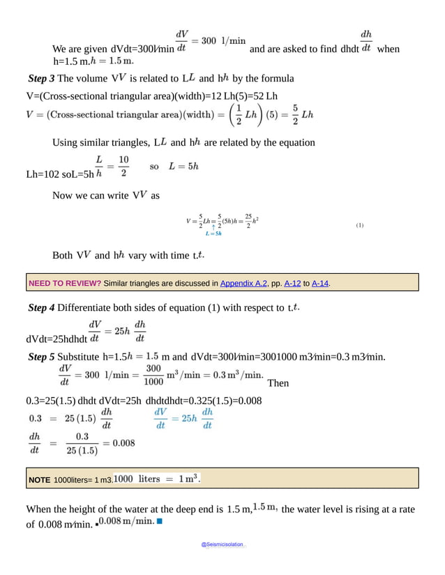
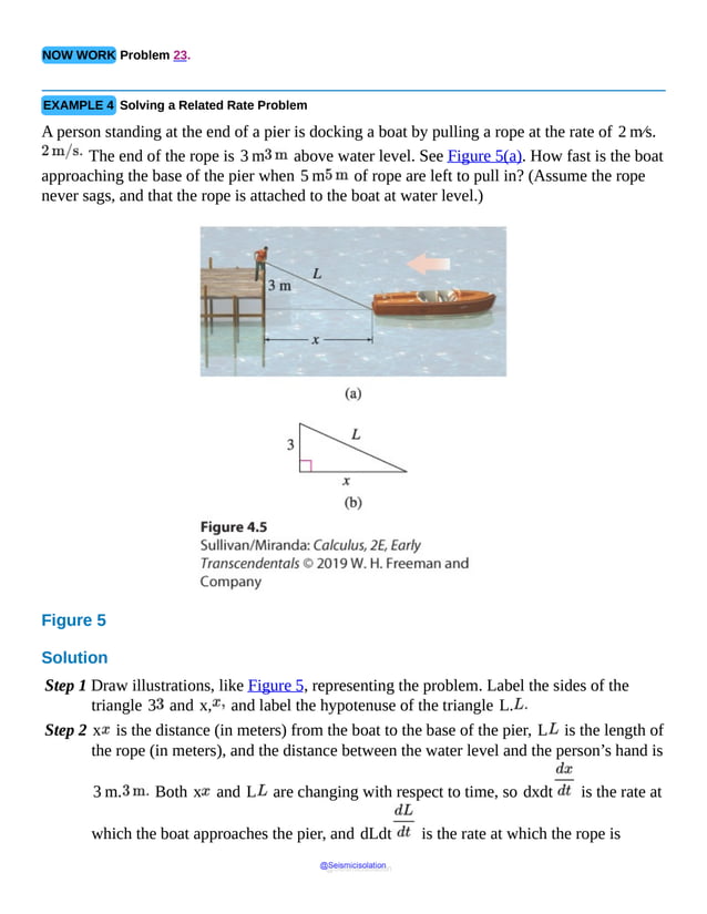
749. container at the constant rate of 16 m3⁄min, how fast is the water level rising
when the water is 8 m deep?
(Hint: The volume V of a cone of radius r and height h is V = 13 πr2h.]
24. Building a Sand Pile Sand is being poured onto the ground, forming a conical pile
whose height equals one-fourth of the diameter of the base. If the sand is falling at the
rate of 20 c m3 ⁄s, how fast is the height of the sand pile increasing when it is
3 cm high?
25. Is There a Leak? A cistern in the shape of a cone 4 m deep and 2 m in diameter
at the top is being filled with water at a constant rate of 3 m3 ⁄min.
a. At what rate is the water rising when the water in the tank is 3 m deep?
b. If, when the water is 3 m deep, it is observed that the water rises at a rate of
0.5 m⁄min, at what rate is water leaking from the tank?
26. Change in Area The vertices of a rectangle are at (0,0), (0,ex), (x,0),
and (x,ex),x> 0. If x increases at the rate of 1 unit per second,
at what rate is the area increasing when x= 10 units?
27. Distance from the Origin An object is moving along the parabola y2=4(3−x).
When the object is at the point (−1,4), its y -coordinate is
increasing at the rate of 3 units per second. How fast is the distance from the object to
the origin changing at that instant?
28. Funneling Liquid A conical funnel 15 cm in diameter and 15 cm deep is
filled with a liquid that runs out at the rate of 5 cm3 ⁄min. At what rate is the
depth of liquid changing when its depth is 8 cm?
@Seismicisolation
@Seismicisolation

750. 29. Baseball A baseball is hit along the third-base line with a speed of 100 ft⁄s. At
what rate is the ball’s distance from first base changing when it crosses third base? See
the figure.
30. Flight of a Falcon A peregrine falcon flies up from its trainer at an angle of 60 ∘
until it has flown 200 ft. It then levels off and continues to fly away. If the
constant speed of the bird is 88 ft⁄s, how fast is the falcon moving away from the
falconer after it is 6 s in flight. See the figure.
Source: http://www.rspb.org.uk
31. Boyle’s Law A gas is said to be compressed adiabatically if there is no gain or loss of
heat. When such a gas is diatomic (has two atoms per molecule), it satisfies the equation
PV1.4=k, where k is a constant, P is the pressure, and V is the volume.
At a given instant, the pressure is 20 kg⁄cm2, the volume is 32 cm3,
and the volume is decreasing at the rate of 2 cm3 ⁄min. At what rate is the
pressure changing?
32. Heating a Plate When a metal plate is heated, it expands. If the shape of the plate is
circular and its radius is increasing at the rate of 0.02 cm⁄s, at what rate is the
@Seismicisolation
@Seismicisolation

751. area of the top surface increasing when the radius is 3 cm?
33. Pollution After a rupture, oil begins to escape from an underwater well. If, as the oil
rises, it forms a circular slick whose radius increases at a rate of 0.42 ft⁄min,
find the rate at which the area of the spill is increasing when the radius is 120 ft.
34. Flying a Kite A girl flies a kite at a height 30 m above her hand. If the kite flies
horizontally away from the girl at the rate of 2 m⁄s, at what rate is the string being
let out when the length of the string released is 70 m? Assume that the string
remains taut.
35. Falling Ladder An 8-m ladder is leaning against a vertical wall. If a person pulls
the base of the ladder away from the wall at the rate of 0.5 m⁄s, how fast is the
top of the ladder moving down the wall when the base of the ladder is
a. 3 m from the wall?
b. 4 m from the wall?
c. 6 m from the wall?
36. Beam from a Lighthouse A light in a lighthouse 2000 m from a straight
shoreline is rotating at 2 revolutions per minute. How fast is the beam moving along
the shore when it passes a point 500 m from the point on the shore opposite the
lighthouse? (Hint: One revolution=2π rad.)
37. Moving Radar Beam A radar antenna, making one revolution every 5 s, is located
on a ship that is 6 km from a straight shoreline. How fast is the radar beam moving
along the shoreline when the beam makes anangle of 45 ∘ with the shore?
38. Tracking a Rocket When a rocket is launched, it is tracked by a tracking dish on the
ground located a distance D from the point of launch. The dish points toward the
rocket and adjusts its angle of elevation θ to the horizontal (ground level) as the rocket
rises. Suppose a rocket rises vertically at a constant speed of 2.0m⁄s, with the
tracking dish located 150 m from the launch point. Find the rate of change of the
angle θ of elevation of the tracking dish with respect to time t (tracking rate) for each
of the following:
a. Just after launch.
b. When the rocket is 100 m above the ground.
c. When the rocket is 1.0 km above the ground.
d. Use the results in (a)–(c) to describe the behavior of the tracking rate as the rocket
climbs higher and higher. What limit does the tracking rate approach as the rocket
gets extremely high?
39. Lengthening Shadow A child, 1 m tall, is walking directly under a street lamp that
@Seismicisolation
@Seismicisolation

752. is 6 m above the ground. If the child walks away from the light at the rate of
20 m⁄min, how fast is the child’s shadow lengthening?
40. Approaching a Pole A boy is walking toward the base of a pole 20 m high at the
rate of 4 km⁄h. At what rate (in meters per second) is the distance from his feet
to the top of the pole changing when he is 5 m from the pole?
41. Riding a Ferris Wheel A Ferris wheel is 50 ft in diameter and its center is located
30 ft above the ground. See the image. If the wheel rotates once every 2 min,
how fast is a passenger rising when he is 42.5 ft above the ground? How fast is he
moving horizontally?
42. Approaching Cars Two cars approach an intersection, one heading east at the rate of
30 km⁄h and the other heading south at the rate of 40 km⁄h. At what
rate are the two cars approaching each other at the instant when the first car is 100 m
from the intersection and the second car is 75 m from the intersection?
Assume the cars maintain their respective speeds.
43. Parting Ways An elevator in a building is located on the fifth floor, which is 25 m
above the ground. A delivery truck is positioned directly beneath the elevator at street
level. If, simultaneously, the elevator goes down at a speed of 5 m⁄s and the truck
pulls away at a speed of 8 m⁄s, how fast will the elevator and the truck be
separating 1 s later? Assume the speeds remain constant at all times.
44. Pulley In order to lift a container 10 m, a rope is attached to the container and,
with the help of a pulley, the container is hoisted. See the figure. If a person holds the
@Seismicisolation
@Seismicisolation

753. end of the rope and walks away from beneath the pulley at the rate of 2 m⁄s, how
fast is the container rising when the person is 5 m away? Assume the end of the rope
in the person’s hand was originally at the same height as the top of the container.
45. Business A manufacturer of precision digital switches has daily cost C and revenue
R, in dollars, of C(x)= 10,000+ 3x and R(x)= 5x− x22000,
respectively, where x is the daily production of switches.
Production is increasing at the rate of 50 switches per day when production is 1000
switches.
a. Find the rate of increase in cost when production is 1000 switches per day.
b. Find the rate of increase in revenue when production is 1000 switches per day.
c. Find the rate of increase in profit when production is 1000 switches per day.
(Hint: Profit = Revenue – Cost)
46. An Enormous Growing Black Hole In December 2011 astronomers announced the
discovery of the two most massive black holes identified to date. The holes appear to be
quasar* remnants, each having a mass equal to 10 billion Suns. Huge black holes
typically grow by swallowing nearby matter, including whole stars. In this way, the size
of the event horizon (the distance from the center of the black hole to the position at
which no light can escape) increases. From general relativity, the radius R of the event
horizon for a black hole of mass m is R= 2Gmc2, where G is the
gravitational constant and c is the speed of light in a vacuum.
a. If one of these huge black holes swallows one Sun-like star per year, at what rate (in
kilometers per year) will its event horizon grow? The mass of the Sun is 1.99×
@Seismicisolation
@Seismicisolation

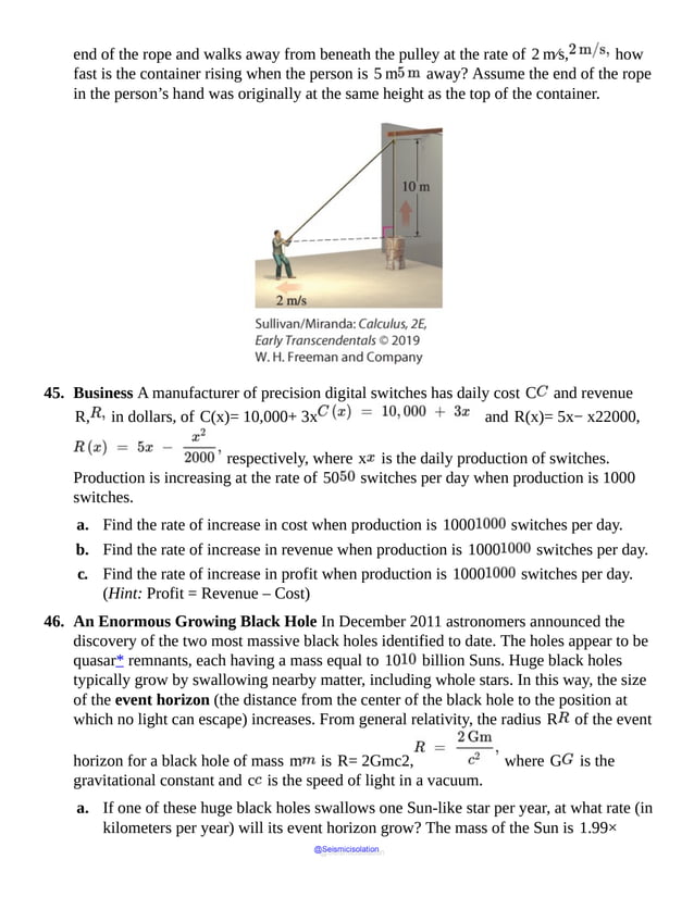
754. 1030 kg, the speed of light in a vacuum is c= 3.00× 108 m⁄s,
and G= 6.67× 10−11 m3 ⁄(kg⋅s2).
b. By what percent does the event horizon change per year?
*A quasar is an astronomical object that emits massive amounts of electromagnetic
radiation.
47. Weight in Space An object that weighs K lb on the surface of Earth weighs
approximately
W(R)=K 39603960+R2
pounds when it is a distance of R mi from Earth’s surface. Find the rate at which
the weight of an object weighing 1000 lb on Earth’s surface is changing when it
is 50 mi above Earth’s surface and is being lifted at the rate of 10 mi⁄s.
48. Pistons In a certain piston engine, the distance x in meters between the center of the
crank shaft and the head of the piston is given by x=cos θ+16− sin2 θ,
where θ is the angle between the crank and the path of
the piston head. See the figure below.
a. If θ increases at the constant rate of 45 rad⁄s, what is the speed of the
piston head when θ= π6?
b. Graph x as a function of θ on the interval [0,π]. Determine the maximum
distance and the minimum distance of the piston head from the center of the crank
shaft.
@Seismicisolation
@Seismicisolation

755. 49. Tracking an Airplane A soldier at an anti-aircraft battery observes an airplane flying
toward him at an altitude of 4500 ft. See the figure. When the angle of elevation
of the battery is 30 ∘, the soldier must increase the angle of elevation by 1 ∘⁄s
to keep the plane in sight. What is the ground speed of the plane?
50. Change in the Angle of Elevation A hot air balloon is rising at a speed of 100 m⁄min.
If an observer is standing 200 m from the lift-off point, what is the
rate of change of the angle of elevation of the observer’s line of sight when the balloon
is 600 m high?
51. Rate of Rotation A searchlight is following a plane flying at an altitude of 3000 ft
in a straight line over the light; the plane’s velocity is 500 mi⁄h. At
what rate is the searchlight turning when the distance between the light and the plane is
5000 ft? See the figure.
52. Police Chase A police car approaching an intersection at 80 ft⁄s spots a
suspicious vehicle on the cross street. When the police car is 210 ft from the
intersection, the policeman turns a spotlight on the vehicle, which is at that time just
crossing the intersection at a constant rate of 60 ft⁄s. See the figure. How fast
must the light beam be turning 2 s later in order to follow the suspicious vehicle?
@Seismicisolation
@Seismicisolation

756. 53. Change in Volume The height h and width x of an open box with a square base are
related to its volume by the formula V = hx2. Discuss how the volume
changes
a. if h decreases with time, but x remains constant.
b. if both h and x change with time.
54. Rate of Change Let y= 2ecos x. If both x and y vary with time in such
a way that y increases at a steady rate of 5 units per second, at what rate is x
changing when x= π2?
Challenge Problems
55. Moving Shadows The dome of an observatory is a hemisphere 60 ft in diameter. A
boy is playing near the observatory at sunset. He throws a ball upward so that its
shadow climbs to the highest point on the dome. How fast is the shadow moving along
the dome 12 s after the ball begins to fall? How did you use the fact that it was sunset
in solving the problem? (Note: A ball falling from rest covers a distance s= 16t2 ft
in t seconds.)
56. Moving Shadows A railroad train is moving at a speed of 15 mi⁄h past a station
800 ft long. The track has the shape of the parabola y2=600x as shown
in the figure. If the sun is just rising in the east, find how fast the shadow S of the
locomotive L is moving along the wall at the instant it reaches the end of the wall.
@Seismicisolation
@Seismicisolation

757. 57. Change in Area The hands of a clock are 2 in and 3 in long. See the figure. As
the hands move around the clock, they sweep out the triangle OAB. At what rate
is the area of the triangle changing at 12:10 p.m.?
58. Distance A train is traveling northeast at a rate of 25 ft⁄s along a track that is
elevated 20 ft above the ground. The track passes over the street below at an angle
of 30 ∘. See the figure. Five seconds after the train passes over the road, a car
traveling east passes under the tracks going 40 ft⁄s. How fast are the train and the
car separating after 3 s?
@Seismicisolation
@Seismicisolation

758. 1. = NOW WORK problem
= Graphing technology recommended
= Computer Algebra System recommended
@Seismicisolation
@Seismicisolation

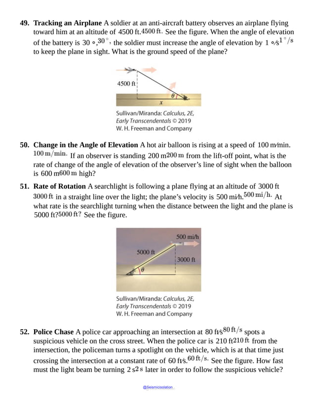
759. 4.2 Maximum and Minimum Values; Critical Numbers
OBJECTIVES When you finish this section, you should be able to:
1 Identify absolute maximum and minimum values and local extreme values of a function
2 Find critical numbers
3 Find absolute maximum and absolute minimum values
Often problems in engineering and economics seek to find an optimal, or best, solution to a
problem. For example, state and local governments try to set tax rates to optimize revenue. If
a problem like this can be modeled by a function, then finding the maximum or the minimum
values of the function solves the problem.
1 Identify Absolute Maximum and Minimum Values and Local Extreme Values
of a Function
Figure 7 illustrates the graph of a function f defined on a closed interval [a,b]. Pay
particular attention to the graph at the numbers x1, x2, and x3. In small open
intervals containing x1 or containing x3 the value of f is greatest at these numbers.
We say that f has local maxima at x1 and x3, and that f(x1) and f(x3) are
local maximum values of f. Similarly, in small open intervals containing x2, the value
of f is least at x2. We say f has a local minimum at x2 and f(x2) is a local
minimum value of f. (“Maxima” is the plural of “maximum”; “minima” is the plural of
“minimum.”)
@Seismicisolation
@Seismicisolation

760. Figure 7
Function
has
local
minima
at
point
(x2,
f
of
x2)
and
local
maxima
at
(x1,
f
of
x1)
in
the
second
quadrant
and
local
On the closed interval [a,b], the largest value of f is f(x3), while the
smallest value of f is f(b). These are called, respectively, the absolute maximum value
and absolute minimum value of f on [a,b].
DEFINITION Absolute Extrema
Let f be a function defined on an interval I. If there is a number u in the interval for
which f(u)≥f(x) for all x in I, then f has an absolute maximum at u
and the number f(u) is called the absolute maximum value of f on I.
If there is a number v in I for which f(v)≤f(x) for all x in I, then f
has an absolute minimum at v and the number f(v) is the absolute minimum value
of f on I.
The values f(u) and f(v) are sometimes called absolute extrema or the
extreme values of f on I. (“Extrema” is the plural of the Latin noun extremum.)
The absolute maximum value and the absolute minimum value, if they exist, are the
largest and smallest values, respectively, of a function f on the interval I. The interval
may be open, closed, or neither. See Figure 8. Contrast this idea with that of a local
maximum value and a local minimum value. These are the largest and smallest values of f
in some open interval in I. The next definition makes this distinction precise.
@Seismicisolation
@Seismicisolation

761. Figure 8 f is defined on an interval I. For all x in I, f(u)≥f(x) and
f(v)≤f(x). f(u) is the absolute maximum value of f. f(v) is the
absolute minimum value of f.
DEFINITION Local Extrema
Let f be a function defined on some interval I and let u and v be numbers in I. If
there is an open interval in I containing u so that f(u)≥f(x) for all x in this
open interval, then f has a local maximum (or relative maximum) at u, and the
number f(u) is called a local maximum value.
Similarly, if there is an open interval in I containing v so that f(v)≤f(x)
for all x in this open interval, then f has a local minimum (or a relative minimum) at
v, and the number f(v) is called a local minimum value.
The term local extreme value describes either a local maximum value of f or a local
minimum value of f.
Figure 9 illustrates the definition.
@Seismicisolation
@Seismicisolation

762. Figure 9 f has a local maximum at u1 and at u2. f has a local minimum at v.
Notice in the definition of a local maximum that the interval that contains u is required
to be open. Notice also in the definition of a local maximum that the value f(u) must be
greater than or equal to all other values of f in this open interval. The word “local” is used
to emphasize that this condition holds on some open interval containing u. Similar remarks
hold for a local minimum. This means that a local extremum cannot occur at the endpoint of
an interval.
EXAMPLE 1 Identifying Maximum and Minimum Values and Local Extreme Values from the Graph of a
Function
Figures 10–15, show the graphs of six different functions. For each function:
a. Find the domain.
b. Determine where the function is continuous.
c. Identify the absolute maximum value and the absolute minimum value, if they exist.
d. Identify any local extreme values.
NEED TO REVIEW? Continuity is discussed in Section 1.3, pp. 102–110.
Solution
@Seismicisolation
@Seismicisolation

763. Figure 10
a. Domain: [0,3π2]
b. Continuous on [0,3π2]
c. Absolute maximum value: f(0)=1
Absolute minimum value: f(π)=−1
d. No local maximum value;
local minimum value: f(π)=−1
@Seismicisolation
@Seismicisolation

764. Figure 11
a. Domain: (−1,3)
b. Continuous on (−1,3)
c. Absolute maximum value: f(0)=1
Absolute minimum value: f(2)=−7
d. Local maximum value: f(0)=1
Local minimum value: f(2)=−7
@Seismicisolation
@Seismicisolation

765. Figure 12
a. Domain: (−1,4]
b. Continuous on (−1,4]
c. No absolute maximum value;
absolute minimum value: f(4)=1
d. No local maximum value;
no local minimum value
@Seismicisolation
@Seismicisolation

766. Figure 13
a. Domain: (0,e)
b. Continuous on (0,e)
c. No absolute maximum value;
no absolute minimum value
d. No local maximum value;
no local minimum value
@Seismicisolation
@Seismicisolation

767. Figure 14
a. Domain: [0,6]
b. Continuous on [0,6] except at x=2
c. Absolute maximum value: f(2)=6
Absolute minimum value: f(6)=−2
d. Local maximum value: f(2)=6
Local minimum value: f(1)=0
@Seismicisolation
@Seismicisolation

768. Figure 15
a. Domain: [−2,2]
b. Continuous on [−2,2] except at x= 0
c. Absolute maximum value: f(−2)= 3, f(2)=3
No absolute minimum value
d. Local maximum value: f(0)=2
No local minimum value
▪
NOW WORK Problem 7.
Example 1 illustrates that a function f can have both an absolute maximum value and an
absolute minimum value, can have one but not the other, or can have neither an absolute
maximum value nor an absolute minimum value. The next theorem provides conditions for
which a function f will always have absolute extrema. Although the theorem seems simple,
the proof requires advanced topics and may be found in most advanced calculus books.
THEOREM Extreme Value Theorem
If a function f is continuous on a closed interval [a,b], then f has an absolute
maximum and an absolute minimum on [a,b].
Look back at Example 1. Figure 10 illustrates a function that is continuous on a closed
interval; it has an absolute maximum and an absolute minimum on the interval. But if a
function is not continuous on a closed interval [a,b], then the conclusion of the Extreme
@Seismicisolation
@Seismicisolation

769. Value Theorem may or may not hold.
For example, the functions graphed in Figures 11–13 are all continuous, but not on a
closed interval:
In Figure 11, the function has both an absolute maximum and an absolute minimum.
In Figure 12, the function has an absolute minimum but no absolute maximum.
In Figure 13, the function has neither an absolute maximum nor an absolute minimum.
On the other hand, the functions graphed in Figures 14 and 15 are each defined on a
closed interval, but neither is continuous on that interval:
In Figure 14, the function has an absolute maximum and an absolute minimum.
In Figure 15, the function has an absolute maximum but no absolute minimum.
NOW WORK Problem 9.
The Extreme Value Theorem is an existence theorem. It states that, if a function is
continuous on a closed interval, then extreme values exist. It does not tell us how to find
these extreme values. Although we can locate both absolute and local extrema given the
graph of a function, we need tools that allow us to locate the extreme values analytically,
when only the function f is known.
Next we examine local extrema more closely. Consider the function y=f(x)
whose graph is shown in Figure 16. There is a local maximum at x1 and a local minimum
at x2. The derivative at these numbers is 0, since the tangent lines to the graph of f at
x1 and x2 are horizontal. There is also a local maximum at x3, where the derivative
fails to exist. The next theorem provides the details.
Figure 16
@Seismicisolation
@Seismicisolation

770. (1)
(2)
(3)
THEOREM Condition for a Local Maximum or a Local Minimum
If a function f has a local maximum or a local minimum at the number c, then either f
′(c)=0 or f′(c) does not exist.
Proof Suppose f has a local maximum at c. Then, by definition,
f(c)≥f(x)
for all x in some open interval containing c. Equivalently,
f(x)−f(c)≤0
The derivative of f at c is
f′(c)=limx→c f(x)−f(c)x−c
provided the limit exists. If this limit does not exist, then f′(c) does not exist and there is
nothing further to prove.
If this limit does exist, then
limx→c− f(x)−f(c)x−c=limx→c+ f(x)−f(c)x−c
In the limit on the left, x < c and f(x)−f(c)≤0, so f(x)−f(c)x−c ≥0
and
limx→c− f(x)−f(c)x−c ≥0
[Do you see why? If the limit were negative, then there would be an open interval about c,
x < c, on which f(x)−f(c)<0; refer to Section 1.6, Example 7, p. 145.]
Similarly, in the limit on the right side of (1), x>c and f(x)−f(c)≤0,
so f(x)−f(c)x−c ≤0 and
limx→c+ f(x)−f(c)x−c ≤0
Since the limits (2) and (3) must be equal, we have
@Seismicisolation
@Seismicisolation

771. f′(c)=limx→c f(x)−f(c)x−c=0
The proof when f has a local minimum at c is similar and is left as an exercise
(Problem 92).
▪
For differentiable functions, the following theorem, often called Fermat’s Theorem, is
simpler.
Theorem If a differentiable function f has a local maximum or a local minimum at c, then f′(c)=0.
In other words, for differentiable functions, local extreme values occur at points where
the tangent line to the graph of f is horizontal.
As the theorems show, the numbers at which a function f′(x)=0 or at which f
′(x) does not exist provide a clue for locating where f has local extrema. But
unfortunately, knowing that f′(c)=0 or that f′ does not exist at c does not
guarantee a local extremum occurs at c. For example, in Figure 17, f′(x3)=0,
but f has neither a local maximum nor a local minimum at x3. Similarly, f′(x4)
does not exist, but f has neither a local maximum nor a local minimum at x4.
Figure 17
Even though there may be no local extrema found at the numbers c for which f′(c)=0
or f′(c) do not exist, the collection of all such numbers provides all the
@Seismicisolation
@Seismicisolation

772. possibilities where f might have local extreme values. For this reason, we call these
numbers critical numbers.
DEFINITION Critical Number
A critical number of a function f is a number c in the domain of f for which either f
′(c)=0 or f′(c) does not exist.
ORIGINS Pierre de Fermat (1601–1665), a lawyer whose contributions to mathematics were made in his spare
time, ranks as one of the great “amateur” mathematicians. Although Fermat is often remembered for his famous
“last theorem,” he established many fundamental results in number theory and, with Pascal, cofounded the
theory of probability. Since his work on calculus was the best done before Newton and Leibniz, he must be
considered one of the principal founders of calculus.
2 Find Critical Numbers
EXAMPLE 2 Finding Critical Numbers
Find any critical numbers of the following functions:
a. f(x)=x3−6x2+9x+2
b. R(x)=1x−2
c. g(x)=(x−2)2⁄3x
d. G(x)=sin x @Seismicisolation
@Seismicisolation

773. Solution a. Since f is a polynomial, it is differentiable at every real number. So, the critical
numbers occur where f′(x)=0.
f′(x)=3x2−12x+9=3(x−1)(x−3)
f′(x)=0 at x=1 and x=3; the numbers 1 and 3 are the critical
numbers of f.
b. The domain of R(x)=1x−2 is {x|x≠2}, and R′(x)=− 1(x−2)2.
R′ exists for all numbers x in the domain of R (remember, 2 is
not in the domain of R ). Since R′ is never 0, R has no critical numbers.
c. The domain of g(x)=(x−2)2⁄3x is {x|x≠0}, and the derivative
of g is
Critical numbers occur where g′(x)=0 or where g′(x) does not exist. Since
g′(6)=0, x=6 is a critical number. Next, g′(x) does not exist where
3x2(x−2)1⁄3=03x2=0or (x−2)1⁄3=0x=0or x=2
We ignore 0 since it is not in the domain of g. The critical numbers of g are 6 and 2.
d. The domain of G is all real numbers. The function G is differentiable on its domain,
so the critical numbers occur where G′(x)=0. G′(x)=cos x and
cos x=0 at x=±π2, ±3π2, ±5π2,…. This function has
infinitely many critical numbers.
▪
NOW WORK Problem 25.
@Seismicisolation
@Seismicisolation

774. We are not yet ready to give a procedure for determining whether a function f has a
local maximum, a local minimum, or neither at a critical number. This requires the Mean
Value Theorem, which is the subject of the next section. However, the critical numbers do
help us find the extreme values of a function f.
3 Find Absolute Maximum and Absolute Minimum Values
The following theorem provides a way to find the absolute extreme values of a function f
that is continuous on a closed interval [a,b].
THEOREM Locating Absolute Extreme Values
Let f be a function that is continuous on a closed interval [a,b]. Then the absolute
maximum value and the absolute minimum value of f are the largest and the smallest
values, respectively, found among the following:
The values of f at the critical numbers in the open interval (a,b)
f(a) and f(b), the values of f at the endpoints a and b
For any function f satisfying the conditions of this theorem, the Extreme Value
Theorem reveals that extreme values exist, and this theorem tells us how to find them.
Steps for Finding the Absolute Extreme Values of a Function f That Is Continuous on a Closed Interval
[a, b]
Step 1 Locate all critical numbers in the open interval (a,b).
Step 2 Evaluate f at each critical number and at the endpoints a and b.
Step 3 The largest value is the absolute maximum value; the smallest value is the absolute
minimum value.
EXAMPLE 3 Finding Absolute Maximum and Minimum Values
Find the absolute maximum value and the absolute minimum value of each function:
a. f(x)=x3−6x2+9x+2 on [0,2]
b. g(x)=(x−2)2⁄3x on [1,10]
Solution a. The function f, a polynomial function, is continuous on the closed interval
[0,2], so the Extreme Value Theorem guarantees that f has an absolute maximum
@Seismicisolation
@Seismicisolation

775. value and an absolute minimum value on the interval. Follow the steps for finding extreme
values.
Step 1 From Example 2a., the critical numbers of f are 1 and 3. We exclude 3, since
it is not in the interval (0,2).
Step 2 Find the value of f at the critical number 1 and at the endpoints 0 and 2:
f(1)=6f(0)=2f(2)=4
Step 3 The largest value 6 is the absolute maximum value of f; the smallest value 2 is
the absolute minimum value of f.
b. The function g is continuous on the closed interval [1,10], so g has an absolute
maximum and an absolute minimum on the interval.
Step 1 From Example 2c., the critical numbers of g are 2 and 6. Both critical numbers
are in the interval (1,10).
Step 2 Evaluate g at the critical numbers 2 and 6 and at the endpoints 1 and 10:
x
g(x)=(x −2)2⁄3x
1
(1 −2)2⁄31=(−1)2⁄3=1
← absolute maximum value
2
(2 −2)2⁄32=0
← absolute minimum value
6
(6 −2)2⁄36=42⁄36 ≈0.42
10
(10 −2)2⁄310=82⁄310=0.4
Step 3 The largest value 1 is the absolute maximum value; the smallest value 0 is the
absolute minimum value.
▪
NOW WORK Problem 49.
For piecewise-defined functions f, we need to look carefully at the number(s) where
the rules for the function change.
EXAMPLE 4 Finding Absolute Maximum and Minimum Values
Find the absolute maximum value and absolute minimum value of the function
@Seismicisolation
@Seismicisolation

776. f(x) ={2x−1 if0 ≤ x ≤2x2−5x +9if2 < x ≤3
Solution The function f is continuous on the closed interval [0,3]. (You should
verify this.) To find the absolute maximum value and absolute minimum value, we follow the
three-step procedure.
Step 1 Find the critical numbers in the open interval (0,3):
On the open interval (0,2): f(x)=2x−1 and f′(x)=2. Since
f′(x)≠0 on the interval (0,2), there are no critical numbers in (0,2).
On the open interval (2,3): f(x)=x2−5x +9 and f′(x)=2x−5.
Solving f′(x)=2x−5=0, we find x=52. Since
52 is in the interval (2,3), 52 is a critical number.
At x=2, the rule for f changes, so we investigate the one-sided limits of f(x)
−f(2)x−2.
limx→2− f(x)−f(2)x−2=limx→2− (2x−1)−3x−2=limx→2− 2x−4x−2=limx→2− 2(x−2)x
−2=2limx→2+ f(x)−f(2)x−2=limx→2+ (x2−5x +9)−3x−2=limx→2+ x2−5x +6x
−2=limx→2+ (x−2)(x−3)x−2=limx→2+ (x−3)=−1
The one-sided limits are not equal, so the derivative does not exist at 2; 2 is a
critical number.
Step 2 Evaluate f at the critical numbers 52 and 2 and at the endpoints 0 and 3.
x f(x)
0 2 ⋅0−1=−1 ← absolute minimum value
@Seismicisolation
@Seismicisolation

777. 2 2 ⋅2−1=3 ← absolute maximum value
52
522−5⋅52 +9=254−252
+9=114
3 32−5 ⋅3 +9=9−15 +9=3 ← absolute maximum value
Step 3 The largest value 3 is the absolute maximum value; the smallest value −1 is the
absolute minimum value.
▪
The graph of f is shown in Figure 18. Notice that the absolute maximum occurs at 2
and at 3.
Figure 18
f(x) ={2x−1 if0 ≤ x ≤2x2−5x +9if2 < x ≤3
NOW WORK Problem 61.
EXAMPLE 5 Constructing a Rain Gutter
@Seismicisolation
@Seismicisolation

778. A rain gutter is to be constructed using a piece of aluminum 12 in. wide. After marking a
length of 4 in. from each edge, the piece of aluminum is bent up at an angle θ, as
illustrated in Figure 19. The area A of a cross section of the opening, expressed as a
function of θ, is
A(θ)=16 sin θ (cos θ +1)0 ≤ θ≤ π2
Figure 19
Find the angle θ that maximizes the area A. (This bend will allow the most water to flow
through the gutter.)
Solution The function A=A(θ) is continuous on the closed interval [0,π2].
To find the angle θ that maximizes A, follow the three-step procedure.
Step 1 Locate all critical numbers in the open interval 0,π2.
A′(θ) =16 sin θ (− sin θ) +16 cos θ (cos θ +1) =16[−sin2 θ +cos2 θ +cos θ] =16[(cos2 θ
−1) +cos2 θ +cos θ] =16[2 cos2 θ +cos θ−1]=16(2 cos θ−1)(cos θ +1)
@Seismicisolation
@Seismicisolation

779. The critical numbers satisfy the equation A′(θ)=0,0 < θ< π2.
16(2 cos θ−1)(cos θ +1)=02 cos θ−1=0 orcos θ +1=0cos θ=12cos θ=−1θ=π3 or 5π3θ=π
Of these solutions, only π3 is in the interval 0,π2. So, π3 is the only critical
number.
Step 2 Evaluate A at the critical number π3 and at the endpoints 0 and π2.
θ A(θ)=16 sin θ (cos θ +1)
0 16 sin 0 (cos 0 +1)=0
π3 16 sin π3 (cos π3 +1)= 16 (32) (12 +1)= 123≈20.785 ← absolute maximum value
π2 16 sin π2 cos π2 +1=16(1)(0 +1)=16
Step 3 If the aluminum is bent at an angle of π3 (60 ∘), the area of the opening is a
maximum. The maximum area is approximately 20.785 in2. ▪
NOW WORK Problem 71.
Application: Physics in Medicine
From physics, the volume V of fluid flowing through a pipe is a function of the radius r
of the pipe and the difference in pressure p at each end of the pipe and is given by
V=kpr4
where k is a constant.
EXAMPLE 6 Analyzing a Cough
Coughing is caused by increased pressure in the lungs and is accompanied by a decrease in
the diameter of the windpipe. See Figure 20. The radius r of the windpipe decreases with
increased pressure p according to the formula r0−r=cp, where r0 is the
@Seismicisolation
@Seismicisolation

780. radius of the windpipe when there is no difference in pressure and c is a positive constant.
The volume V of air flowing through the windpipe is
V=kpr4
where k is a constant. Find the radius r that allows the most air to flow through the
windpipe. Restrict r so that 0 < r02 ≤ r ≤ r0.
Figure 20
Solution Since p= r0−rc, we can express V as a function of r:
V=V(r)=k r0−rcr4=kr0cr4−kc r5r02 ≤ r ≤ r0
Now find the absolute maximum of V on the interval [r02,r0].
V′(r)=4k r0cr3−5kcr4=kc r3(4r0−5r)
@Seismicisolation
@Seismicisolation

781. The only critical number in the interval r02,r0 is r=4r05.
Evaluate V at the critical number and at the endpoints, r02 and r0.
r
V(r)=kr0−rcr4
r02
kr0−r02cr024=k r0532c
≈ 0.031 k r05c
4r05
kr0−4r05c4r054=kc ⋅ 44 r0555=256 kr053125c
≈ 0.082 k r05c
r0 0
The largest of these three values is 256 kr053125c. So, the maximum air flow
occurs when the radius of the windpipe is 4r05, that is, when the windpipe contracts by
20%. ▪
4.2 Assess Your Understanding
Concepts and Vocabulary
1. True or False Any function f that is defined on a closed interval [a,b] will have
both an absolute maximum value and an absolute minimum value.
2. Multiple Choice A number c in the domain of a function f is called a(n)
[(a) extreme value (b) critical number (c) local number] of f if either f′(c) = 0
or f′(c) does not exist.
3. True or False At a critical number, there is a local extreme value.
4. True or False If a function f is continuous on a closed interval [a,b], then its
absolute maximum value is found at a critical number .
5. True or False The Extreme Value Theorem tells us where the absolute maximum and
@Seismicisolation
@Seismicisolation

782. absolute minimum can be found.
6. True or False If f is differentiable on the interval (0,4) and f′(2) = 0,
then f has a local maximum or a local minimum at 2.
Skill Building
In Problems 7 and 8, use the graphs below to determine whether the function f has an
absolute extremum and/or a local extremum or neither at x1, x2, x3, x4, x5,
x6, x7, and x8.
7.
8.
In Problems 9–12, provide a graph of a continuous function f that has the following
properties:
9. domain [0,8], absolute maximum at 0, absolute minimum at 3, local
minimum at 7
10. domain [−5,5], absolute maximum at 3, absolute minimum at −3
@Seismicisolation
@Seismicisolation

783. 11. domain [3,10] and has no local extreme points
12. no absolute extreme values, is differentiable at 4 and has a local minimum at 4, is
not differentiable at 0, but has a local maximum at 0
In Problems 13–36, find the critical numbers, if any, of each function.
13. f(x) = x2−8x
14. f(x)=1−6x +x2
15. f(x)=x3−3x2
16. f(x)=x3−6x
17. f(x)=x4−2x2 +1
18. f(x)=3x4−4x3
19. f(x)=x2⁄3
20. f(x)=x1⁄3
21. f(x) = 2x
22. f(x)=4−x
23. f(x) = x +sin x, 0 ≤ x ≤ π
24. f(x) = x−cos x, −π2 ≤ x ≤ π2
25. f(x) = x1−x2
26. f(x)=x22−x
27. f(x)=x2x−1
28. f(x)=xx2−1
29. f(x)=(x +3)2(x−1)2⁄3
30. f(x)=(x−1)2(x +1)1⁄3
31. f(x)=(x−3)1⁄3x−1
@Seismicisolation
@Seismicisolation

784. 32. f(x)=(x +3)2⁄3x +1
33. f(x)=x2−93x
34. f(x)=4−x23x
35.
f(x) ={3x if 0 ≤ x < 14−x if 1 ≤ x ≤ 2
36.
f(x) ={x2 if 0 ≤ x < 11−x2if1 ≤ x ≤2
In Problems 37–64, find the absolute maximum value and absolute minimum value of each
function on the indicated interval. Notice that the functions in Problems 37–58 are the same
as those in Problems 13–34 above.
37. f(x) = x2−8x on [−1,10]
38. f(x) = 1−6x + x2 on [0,4]
39. f(x) = x3−3x2 on [1,4]
40. f(x) = x3−6x on [−1,1]
41. f(x) = x4−2x2 + 1 on [0,2]
42. f(x) = 3x4−4x3 on [−2,0]
43. f(x) = x2⁄3 on [−1,1]
44. f(x) = x1⁄3 on [−1,1]
45. f(x) = 2x on [1,4]
46. f(x) = 4−x on [0,4]
47. f(x) = x +sin x on [0,π]
48. f(x) = x−cos x on [−π2,π2]
@Seismicisolation
@Seismicisolation

785. 49. f(x) = x1−x2 on [−1,1]
50. f(x) = x22−x on [0,2]
51. f(x) = x2x−1 on [−1,12]
52. f(x) = xx2−1 on [−12,12]
53. f(x) = (x + 3)2(x−1)2⁄3 on [−4,5]
54. f(x) = (x−1)2(x + 1)1⁄3 on [−2,7]
55. f(x) = (x−3)1⁄3x−1 on [2,11]
56. f(x) = (x + 3)2⁄3x +1 on [−4, −2]
57. f(x) = x2−93x on [3,6]
58. f(x)=4−x23x on [−4, −1]
59. f(x)=ex−3x on [0,1]
60. f(x)=ecos x on [−π,2π]
61.
f(x)={2x+1 if 0 ≤x<13x if 1 ≤x≤3
62.
f(x)={x+3 if −1≤x≤22x+1 if 2<x≤4
63.
f(x)={x2 if −2≤x<1x3 if 1≤x≤2
@Seismicisolation
@Seismicisolation

786. 64.
f(x)={x+2 if −1≤x<02−x if 0≤x≤1
Applications and Extensions
In Problems 65–68, for each function f :
a. Find the derivative f′.
b. Use technology to find the critical numbers of f.
c. Graph f and describe the behavior of f suggested by the graph at each critical
number.
65. f(x)=3x4−2x3−21x2+36x
66. f(x)=x2+2x−2x
67. f(x)=(x2−5x+2)x+5x2+2
68. f(x)=(x2−9x+16)x+3x2−4x+6
In Problems 69 and 70, for each function f:
a. Find the derivative f′.
b. Use technology to find the absolute maximum value and the absolute minimum value of f
on the closed interval [0,5].
c. Graph f. Are the results from (b) supported by the graph?
69. f(x)=x4−12.4x3+49.24x2−68.64x
70. f(x)=e−xsin (2x)+e−x⁄2 cos (2x)
71. Cost of Fuel A truck has a top speed of 75 mi⁄h, and when traveling at the rate
of x mi⁄h, it consumes fuel at the rate of 1200 2500x+x gallon
per mile. If the price of fuel is $3.60⁄gal, the cost C (in dollars) of driving
200 mi is given by
@Seismicisolation
@Seismicisolation

787. C(x)=(3.60)2500x+x
a. What is the most economical speed for the truck to travel? Use the interval [10,75].
b. Graph the cost function C.
72. Trucking Costs If the driver of the truck in Problem 71 is paid $28.00 per hour
and wages are added to the cost of fuel, what is the most economical speed for the truck
to travel?
73. Projectile Motion An object is propelled upward at an angle θ, 45 ∘<θ<90 ∘,
to the horizontal with an initial velocity of v 0ft⁄s from the base
of an inclined plane that makes an angle of 45 ∘ to the horizontal. See the
illustration below. If air resistance is ignored, the distance R, in feet, that the object
travels up the inclined plane is given by the function
R(θ)=v02216 cos θ (sin θ−cos θ)
a. Find the angle θ that maximizes R. What is the maximum value of R?
b. Graph R=R(θ), 45 ∘≤θ≤90 ∘, using v0=32 ft⁄s.
c. Does the graph support the result from (a)?
74. Height of a Cable An electric cable is suspended between two poles of equal height
that are 20 m apart, as illustrated in the figure. The shape of the cable is modeled
by the equation y=10 cosh x10+15 with the x -axis placed along
the ground and the two poles at (−10,0) and (10,0). What is the height
of the cable at its lowest point? @Seismicisolation
@Seismicisolation

788. 75. Golf Ball Speed The fastest speed of a golf ball on record is 97.05 m⁄s (217.1 mi⁄h
). It was hit by Ryan Winther at the Orange County National Driving Range in
Orlando, Florida on January 13, 2013. When a ball is hit at an angle θ to the
horizontal, 0 ∘≤θ≤90 ∘, and lands at the same level from which it was hit,
the horizontal range R of the ball is given by R=2v02gsin θ cos θ,
where v0 is the initial speed of the ball and g=9.8 m⁄s2 is the
acceleration due to gravity.
a. Show that the golf ball achieves its maximum range if the golfer hits it at an angle
of 45 ∘.
b. What is the maximum range that could be achieved by the record golf ball speed?
Source: http://www.guinnessworldrecords.com.
76. Optics When light goes through a thin slit, it spreads out (diffracts). After passing
through the slit, the intensity I of the light on a distant screen is given by I=I0sin αα2,
where I0 is the original intensity of the light and α depends on the
angle away from the center.
a. What is the intensity of the light as α→0?
b. Show that the bright spots, that is, the places where the intensity has a local
maximum, occur when tan α=α.
c. Is the intensity of the light the same at each bright spot?
Economics In Problems 77 and 78, use the following discussion:
In determining a tax rate on consumer goods, the government is always faced with the
@Seismicisolation
@Seismicisolation

789. question, ”What tax rate produces the largest tax revenue?” Imposing a tax may cause
the price of the goods to increase and reduce the demand for the product. A very large
tax may reduce the demand to zero, with the result that no tax is collected. On the other
hand, if no tax is levied, there is no tax revenue at all. (Tax revenue R is the product of
the tax rate t times the actual quantity q, in dollars, consumed.)
77. The government has determined that the relationship between the quantity q of a
product consumed and the related tax rate t is t=27−3q2. Find the tax
rate that maximizes tax revenue. How much tax is generated by this rate?
78. On a particular product, government economists determine that the relationship between
the tax rate t and the quantity q consumed is t+3q2=18. Find the tax rate
that maximizes tax revenue and the revenue generated by the tax.
79. Catenary A town hangs strings of holiday lights across the road between utility poles.
Each set of poles is 12 m apart. The strings hang in catenaries modeled by
y=15 cosh x15−10 with the poles at (±6,0 ). What is the height
of the string of lights at its lowest point?
80. Harmonic Motion An object of mass 1 kg moves in simple harmonic motion, with
an amplitude A=0.24 m and a period of 4 s. The position s of the object
is given by s(t)=A cos (ωt), where t is the time in seconds.
a. Find the position of the object at time t and at time t=0.5 s.
b. Find the velocity v=v(t) of the object.
c. Find the velocity of the object when t=0.5 s.
d. Find the acceleration a=a(t) of the object.
e. Use Newton’s Second Law of Motion, F=ma, to find the magnitude and
direction of the force acting on the object when t=0.5 s.
f. Find the minimum time required for the object to move from its initial position to
the point where s=−0.12 m.
g. Find the velocity of the object when s=−0.12 m.
81.
a. Find the critical numbers of f(x)=x33−0.055x2+0.0028x−4.
b. Find the absolute extrema of f on the interval [−1,1].
c. Graph f on the interval [−1,1].
@Seismicisolation
@Seismicisolation

790. 82. Extreme Value
a. Find the minimum value of y=x−cosh−1x.
b. Graph y=x−cosh−1 x.
83. Locating Extreme Values Find the absolute maximum value and the absolute minimum
value of f(x)=1+x2+|x−2 | on [0,3], and determine
where each occurs.
84. The function f(x)=Ax2+Bx+C has a local minimum at 0, and
its graph contains the points (0,2) and (1,8). Find A, B, and C.
85.
a. Determine the domain of the function f(x)=[(16−x2)(x2−9)]1⁄2.
b. Find the absolute maximum value of f on its domain.
86. Absolute Extreme Values Without finding them, explain why the function f(x)=x(2−x)
must have an absolute maximum value and an absolute minimum
value. Then find the absolute extreme values in two ways (one with and one without
calculus).
87. Put It Together If a function f is continuous on the closed interval [a,b], which
of the following is necessarily true?
a. f is differentiable on the open interval (a,b).
b. If f(u) is an absolute maximum value of f, then f′(u)=0.
c. limx→c f(x)=f(limx→c x) for a<c<b.
d. f′(x)=0, for some x, a≤x≤b.
e. f has an absolute maximum value on [a,b].
88. Write a paragraph that explains the similarities and differences between an absolute
extreme value and a local extreme value.
89. Explain in your own words the method for finding the extreme values of a continuous
function that is defined on a closed interval.
90. A function f is defined and continuous on the closed interval [a,b]. Why can’t
f(a) be a local extreme value on [a,b]?
91. Show that if f has a local minimum at c, then g(x)=−f(x) has a local
@Seismicisolation
@Seismicisolation

791. maximum at c.
92. Show that if f has a local minimum at c, then either f′(c)=0 or f′(c)
does not exist.
Challenge Problem
93.
a. Prove that a rational function of the form f(x)=ax2n+bcxn+d,
n≥1 an integer, has at most five critical numbers.
b. Give an example of such a rational function with exactly five critical numbers.
1. = NOW WORK problem
= Graphing technology recommended
= Computer Algebra System recommended
@Seismicisolation
@Seismicisolation

792. 4.3 The Mean Value Theorem
OBJECTIVES When you finish this section, you should be able to:
1 Use Rolle’s Theorem
2 Work with the Mean Value Theorem
3 Identify where a function is increasing and decreasing
In this section, we prove several theorems. The most significant of these, the Mean Value
Theorem, is used to develop tests for locating local extreme values. To prove the Mean Value
Theorem, we need Rolle’s Theorem.
ORIGINS Michel Rolle (1652–1719) was a French mathematician whose formal education was limited to
elementary school. At age 24, he moved to Paris and married. To support his family, Rolle worked as an
accountant, but he also began to study algebra and became interested in the theory of equations. Although
Rolle is primarily remembered for the theorem proved here, he was also the first to use the notation n for
the n th root.
1 Use Rolle’s Theorem
THEOREM Rolle’s Theorem
Let f be a function defined on a closed interval [a,b]. If:
f is continuous on [a,b],
f is differentiable on (a,b), and
f(a)=f(b),
then there is at least one number c in the open interval (a,b) for which f′(c)=0.
Before we prove Rolle’s Theorem, notice that the graph in Figure 21 meets the three
conditions of Rolle’s Theorem and has at least one number c at which F′(c)=0.
@Seismicisolation
@Seismicisolation

793. Figure 21
In contrast, the graphs in Figure 22 show that the conclusion of Rolle’s Theorem may not
hold when one or more of the three conditions are not met.
Figure 22
Proof Because f is continuous on a closed interval [a,b], the Extreme Value Theorem
guarantees that f has an absolute maximum value and an absolute minimum value on [a,b].
There are two possibilities:
1. If f is a constant function on [a,b], then f′ (x)=0 for all x in (a,b).
2. If f is not a constant function on [a,b], then, because f(a)=f(b), either
the absolute maximum or the absolute minimum occurs at some number c in the open
interval (a,b). Then f(c) is a local maximum value (or a local minimum value),
@Seismicisolation
@Seismicisolation

794. and, since f is differentiable on (a,b), f′(c)=0. ▪
EXAMPLE 1 Using Rolle’s Theorem
Find the x -intercepts of f(x)=x2−5x+6, and show that f′(c)=0
for some number c in the open interval formed by the two x -intercepts. Find c.
Solution At the x -intercepts, f(x)=0.
f(x)=x2−5x+6=(x−2)(x−3)=0
So, x=2 and x=3 are the x -intercepts of the graph of f, and f(2)=f(3)=0.
Since f is a polynomial, it is continuous on the closed interval [2,3] formed by the
x -intercepts and is differentiable on the open interval (2,3). The three conditions of
Rolle’s Theorem are satisfied, guaranteeing that there is a number c in the open interval
(2,3) for which f′(c)=0. Since f′(x)=2x−5, the number c for
which f′(x)=0 is c=52. ▪
See Figure 23 for the graph of f.
Figure 23 f(x)=x2−5x+6
NOW WORK Problem 9.
2 Work with the Mean Value Theorem
The importance of Rolle’s Theorem is that it can be used to obtain other results, many of
which have wide-ranging application. Perhaps the most important of these is the Mean Value
@Seismicisolation
@Seismicisolation

795. (1)
Theorem, sometimes called the Theorem of the Mean for Derivatives.
A geometric example helps explain the Mean Value Theorem. Consider the graph of a
function f that is continuous on a closed interval [a,b] and differentiable on the open
interval (a,b), as illustrated in Figure 24. Then there is at least one number c between
a and b at which the slope f′(c) of the tangent line to the graph of f equals the slope
of the secant line joining the points A=(a,f(a)) and B=(b,f(b)).
That is, there is at least one number c in the open interval (a,b) for which
f′(c)=f(b)−f(a)b−a
Figure 24 The tangent line at (c,f(c)) is parallel to the secant line from A to
B.
THEOREM Mean Value Theorem
Let f be a function defined on a closed interval [a,b]. If
f is continuous on [a,b]
f is differentiable on (a,b)
then there is at least one number c in the open interval (a,b) for which
f′(c)=f(b)−f(a)b−a
@Seismicisolation
@Seismicisolation

796. Proof The slope msec of the secant line containing the points (a,f(a)) and
(b,f(b)) is
msec=f(b)−f(a)b−a
Then using the point (a,f(a)) and the point-slope form of an equation of a line, an
equation of this secant line is
y−f(a)=f(b)−f(a)b−a (x−a)y=f(a)+f(b)−f(a)b−a (x−a)
Now construct a function g that satisfies the conditions of Rolle’s Theorem, by defining g
as
for all x on [a,b].
NOTE The function g has a geometric significance: Its value equals the vertical distance from the graph of
y=f(x) to the secant line joining (a,f(a)) to (b,f(b)). See Figure 25.
Figure 25
@Seismicisolation
@Seismicisolation

797. Since f is continuous on [a,b] and differentiable on (a,b), it follows that g
is also continuous on [a,b] and differentiable on (a,b). Also,
g(a)=f(a)−[f(a)+f(b)−f(a)b−a (a−a)]=0g(b)=f(b)−[f(a)+f(b)−f(a)b−a (b−a)]=0
Now, since g satisfies the three conditions of Rolle’s Theorem, there is a number c in
(a,b) at which g′(c)=0. Since f(a) and f(b)−f(a)b−a are
constants, the derivative of g, from Equation (2) above, is given by
g′(x)=f′(x)−ddx[f(a)+f(b)−f(a)b−a (x−a)]=f′(x)−f(b)−f(a)b−a
Now evaluate g′ at c and use the fact that g′(c)=0.
g′(c)=f′(c)−[f(b)−f(a)b−a]=0f′(c)=f(b)−f(a)b−a ▪
The Mean Value Theorem is another example of an existence theorem. It does not tell us
how to find the number c; it merely states that at least one number c exists. Often, the
number c can be found.
EXAMPLE 2 Verifying the Mean Value Theorem
a. Verify that the function f(x)=x3−3x+5, −1≤x≤1 satisfies
the conditions of the Mean Value Theorem.
b. Find the number(s) c guaranteed by the Mean Value Theorem.
c. Interpret the number(s) geometrically.
Solution a. Since f is a polynomial function, f is continuous on the closed interval [−1,1]
and differentiable on the open interval (−1,1). The conditions of the Mean
Value Theorem are met.
b. Evaluate f at the endpoints −1 and 1 and then find F′(x).
@Seismicisolation
@Seismicisolation

798. f(−1)=7f(1)=3and f′(x)=3x2−3
The number(s) c in the open interval (−1,1) guaranteed by the Mean Value
Theorem satisfy the equation
f′(c)=f(1)−f(−1)1−(−1)3c2−3=3−71−(−1)=−42=−23c2=1c=13=33 or c=−13=−33
There are two numbers in the interval (−1,1) that satisfy the Mean Value
Theorem.
c. At each number, −33 and 33, the slope of the tangent line to the graph of f
equals the slope of the secant line connecting the points (−1,7 ) and (1,3 ). That is,
mtan=F′ −33=F′ 33=−2andmsec=f(1)−f(−1)1−(−1)=3−72=−2
The tangent lines and the secant line are parallel.
See Figure 26.
▪
@Seismicisolation
@Seismicisolation

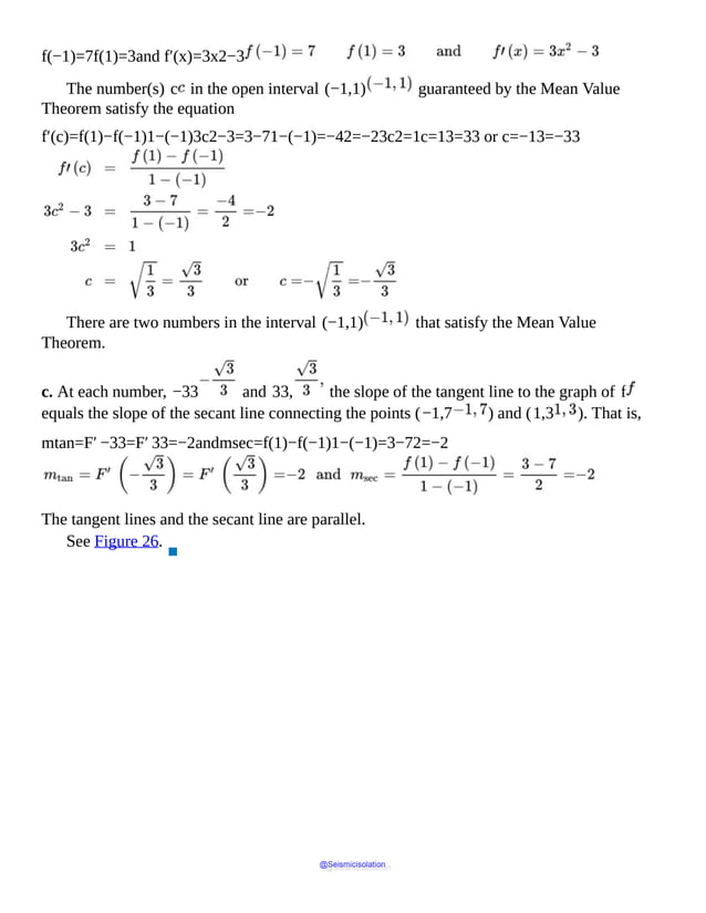
799. Figure 26 f(x)=x3−3x+5, −1≤x≤1
NOW WORK Problem 25.
The Mean Value Theorem can be applied to rectilinear motion. Suppose the position
function s=f(t) models the signed distance s of an object from the origin at time t.
If f is continuous on [a,b] and differentiable on (a,b), the Mean Value
Theorem tells us that there is at least one time t at which the velocity of the object equals its
average velocity.
Let t1 and t2 be two distinct times in [a,b]. Then
Average velocity over [t1,t2]=f(t2)−f(t1)t2−t1Instantaneous velocity v(t)=dsdt=f′(t)
The Mean Value Theorem states there is a time t0 in the interval (t1,t2) for which
f′(t0)=f(t2)−f(t1)t2−t1
@Seismicisolation
@Seismicisolation

800. That is, the velocity at time t0 equals the average velocity over the interval [t1,t2].
EXAMPLE 3 Applying the Mean Value Theorem to Rectilinear Motion
Use the Mean Value Theorem to show that a car that travels 110 mi in 2 h must have
had a speed of 55 miles per hour (mi⁄h ) at least once during the 2 h.
Solution Let s=f(t) represent the distance s the car has traveled after t hours. Its
average velocity during the time period from 0 to 2 h is
Average velocity=f(2)−f(0)2−0=110−02−0=55 mi/h
Using the Mean Value Theorem, there is a time t0, 0<t0<2, at which
f′(t0)=f(2)−f(0)2−0=55
That is, the car had a velocity of 55 mi⁄h at least once during the 2 h period.
▪
NOW WORK Problem 57.
The following corollaries are consequences of the Mean Value Theorem.
COROLLARY
If a function f is continuous on the closed interval [a,b] and is differentiable on the open interval (a,b),
and if f′(x)=0 for all numbers x in (a,b), then f is constant on (a,b).
IN WORDS If f′(x)=0 for all numbers in (a,b), then f is a constant function on the interval
(a,b ).
Proof To show that f is a constant function, we must show that f(x1)=f(x2)
for any two numbers x1 and x2 in the interval (a,b).
Suppose x1<x2. The conditions of the Mean Value Theorem are satisfied on the
interval [x1,x2], so there is a number c in this interval for which
f′(c)=f(x2)−f(x1)x2−x1
@Seismicisolation
@Seismicisolation

801. Since f′(c)=0 for all numbers in (a,b), we have
0=f(x2)−f(x1)x2−x10=f(x2)−f(x1)f(x1)=f(x2) ▪
Applying the corollary to rectilinear motion, if the velocity v of an object is zero over
an interval (t1,t2), then the object does not move during this time interval.
IN WORDS If an object in rectilinear motion has velocity v=0, then the object is at rest.
COROLLARY
If the functions f and g are differentiable on an open interval (a,b) and if f′(x)=g′(x)
for all numbers x in (a,b), then there is a number C for which f(x)=g(x)+C on
(a,b).
Proof We define the function h so that h(x)=f(x)−g(x). Then h is
differentiable since it is the difference of two differentiable functions, and
h′(x)=F′(x)−g′(x)=0
IN WORDS If two functions f and g have the same derivative, then the functions differ by a constant, and
the graph of f is a vertical shift of the graph of g.
Since h′(x)=0 for all numbers x in the interval (a,b), h is a constant
function and we can write
h(x)=f(x)−g(x)=Cfor some number C
That is,
f(x)=g(x)+C ▪
3 Identify Where a Function Is Increasing and Decreasing
A third corollary that follows from the Mean Value Theorem gives us a way to determine
where a function is increasing and where a function is decreasing. Recall that functions are
increasing or decreasing on intervals, either open or closed or half-open or half-closed.
NEED TO REVIEW? Increasing and decreasing functions are discussed in Section P.1, pp. 11–12.
@Seismicisolation
@Seismicisolation

802. COROLLARY Increasing/Decreasing Function Test
Let f be a function that is differentiable on the open interval (a,b):
If f′(x)>0 on (a,b), then f is increasing on (a,b).
If f′(x)<0 on (a,b), then f is decreasing on (a,b).
The proof of the first part of the corollary is given here. The proof of the second part is
left as an exercise. See Problem 82.
Proof Since f is differentiable on (a,b), it is continuous on (a,b). To show that
f is increasing on (a,b), choose two numbers x1 and x2 in (a,b), with
x1<x2. We need to show that f(x1)<f(x2).
Since x1 and x2 are in (a,b), f is continuous on the closed interval [x1,x2]
and differentiable on the open interval (x1,x2). By the Mean Value
Theorem, there is a number c in the interval (x1,x2) for which
f′(c)=f(x2)−f(x1)x2−x1
Since f′(x)>0 for all x in (a,b), it follows that f′(c)>0. Since
x1<x2, then x2−x1>0. As a result,
f(x2)−f(x1)>0f(x1)<f(x2)
So, f is increasing on (a,b). ▪
There are a few important observations to make about the Increasing/Decreasing
Function Test:
In using the Increasing/Decreasing Function Test, we determine open intervals on
which the derivative is positive or negative.
Suppose f is continuous on the closed interval [a,b] and differentiable on the
open interval (a,b).
If f′(x)>0 on (a,b), then f is increasing on the closed interval
[a,b].
@Seismicisolation
@Seismicisolation

803. If f′(x)<0 on (a,b), then f is decreasing on the closed interval
[a,b].
The Increasing/Decreasing Function Test is valid if the interval (a,b) is (−∞,b)
or (a,∞) or (−∞,∞).
EXAMPLE 4 Identifying Where a Function Is Increasing and Decreasing
Determine where the function f(x)=2x3−9x2+12x−5 is
increasing and where it is decreasing.
NEED TO REVIEW? Solving inequalities is discussed in Appendix A.1, pp. A-5 to A-8.
Solution The function f is a polynomial so f is continuous and differentiable at every
real number. We find f′.
f′(x)=6x2−18x+12=6(x−2)(x−1)
The Increasing/Decreasing Function Test states that f is increasing on intervals where f
′(x)>0 and that f is decreasing on intervals where f′(x)<0. We solve
these inequalities by using the numbers 1 and 2 to form three intervals on the x -axis, as
shown in Figure 27. Then we determine the sign of f′(x) on each interval, as shown in
Table 1.
Figure 27
TABLE 1
Interval
Sign of x−
1
Sign of x−
2
Sign of f′(x)=6(x− 2)(x−
1)
Conclusion
(−∞,1) Negative
(−)
Negative
(−)
Positive (+)
f is
increasing
(1,2)
Positive Negative
Negative (−) f is
@Seismicisolation
@Seismicisolation

804. (+) (−)
decreasing
(2,∞) Positive (+) Positive (+) Positive (+) f is increasing
We conclude that f is increasing on the intervals (−∞,1) and (2,∞), and
f is decreasing on the interval (1,2). Since f is continuous on its domain, f is
increasing on the intervals (−∞,1] and [2,∞) and is decreasing on the interval
[1,2]. ▪
Figure 28 shows the graph of f. Notice that the graph of f has horizontal tangent lines
at the points (1,0) and (2,−1 ).
Figure 28 f(x)=2x3−9x2+12x−5
NOW WORK Problem 31.
EXAMPLE 5 Identifying Where a Function Is Increasing and Decreasing
Determine where the function f(x)=(x2−1)2⁄3 is increasing and where it is
decreasing.
Solution f is continuous for all real numbers x, and
@Seismicisolation
@Seismicisolation

805. f′(x)=23 (x2−1)−1⁄3(2x)= 4x3(x2−1)1⁄3
The critical numbers of f are −1,0,1.
The Increasing/Decreasing Function Test states that f is increasing on intervals where f
′(x)>0 and decreasing on intervals where f′(x)<0. We solve these
inequalities by using the critical numbers −1, 0, and 1 to form four intervals on the x-
axis: (−∞, −1), (−1, 0 ), (0, 1), and (1, ∞ ) as shown in Table 2.
TABLE 2
Interval
Sign of
4x
Sign of (x2−
1)1⁄3
Sign of f′(x)= 4x3(x2−
1)1⁄3
Conclusion
(−∞,
−1)
Negative
(−)
Positive (+) Negative (−)
f is decreasing on (−∞,
−1)
(−1,0)
Negative
(−)
Negative (−) Positive (+)
f is increasing on
(−1,0)
(0,1)
Positive
(+)
Negative (−) Negative (−)
f is decreasing on
(0,1)
(1,∞)
Positive
(+)
Positive (+) Positive (+)
f is increasing on
(1,∞)
Then we determine the sign of f′ in each interval. We conclude that f is increasing on
the intervals (−1,0) and (1,∞) and that f is decreasing on the intervals (−∞,
−1) and (0,1).
Since f is continuous on its domain, f is increasing on the intervals [−1,0 ] and
[1,∞) and is decreasing on the intervals (−∞,−1] and [0,1] .
▪
Figure 29 shows the graph of f. Since f′(0)=0, the graph of f has a
horizontal tangent line at the point (0,1). Notice that f′ does not exist at ±1.
Since f′ becomes unbounded at −1 and 1, the graph of f has vertical tangent lines at
the points (−1,0) and (1,0), both of which are cusps.
@Seismicisolation
@Seismicisolation

806. Figure 29 f(x)=(x2−1)2⁄3
NOW WORK Problem 37.
EXAMPLE 6 Obtaining Information About the Graph of a Function from the Graph of Its Derivative
Suppose f is a function that is continuous for all real numbers. The graph of its derivative
function F′ is shown in Figure 30.
Figure 30 The graph of y=F′(x)
a. What is the domain of the derivative function F′?
b. List the critical numbers of f.
c. At what numbers x, if any, does the graph of f have a horizontal tangent line?
@Seismicisolation
@Seismicisolation

807. d. At what numbers x, if any, does the graph of f have a vertical tangent line?
e. At what numbers x, if any, does the graph of f have a corner?
f. On what intervals is the graph of f increasing?
g. On what intervals is the graph of f decreasing?
Solution a. The domain of F′ is the set of all real numbers except 0 and 2.
b. A critical number of f is a number c in the domain of f for which either F′(c)=0
or F′(c) doesn’t exist.
F′(x)=0 where the graph of F′ crosses the x -axis, namely at −2 and 4.
F′(x) does not exist for x=0 and x=2.
The critical numbers of f are −2, 0, 2, and 4.
c. The graph of f has a horizontal tangent line when its slope is zero, namely, at x=−2
and x=4.
d. The graph of f has a vertical tangent line where the derivative F′ is unbounded. This
occurs at x=0.
e. From the graph of F′ we see that the derivative has unequal one-sided limits at x=2.
As x approaches 2 from the left, the derivative is 2, and as x approaches 2 from
the right, the derivative is 1. This means the graph of f has a corner at x=2.
f. The graph of f is increasing when F′(x)>0; that is, when the graph of F′ is
above the x -axis. This occurs on the intervals (−2,0) and (0,4 ). Since f is
continuous for all real numbers, f is continuous on [−2,4].
g. The graph of f is decreasing when F′(x)<0; that is, when the graph of f′ is
below the x -axis. This occurs on the intervals (−∞,−2) and (4,∞). ▪
NOW WORK Problem 47.
Application: Agricultural Economics
EXAMPLE 7 Determining Crop Yield*
A variation of the von Liebig model states that the yield f(x) of a plant, measured in
bushels, responds to the amount x of potassium in a fertilizer according to the following
square root model:
@Seismicisolation
@Seismicisolation

808. f(x)=−0.057−0.417x+0.852x
For what amounts of potassium will the yield increase? For what amounts of potassium will
the yield decrease?
Solution The yield is increasing when f′(x)>0.
f′(x)=−0.417+0.426x=−0.417x+0.426x
Now f′(x)>0 when
−0.417x+0.426>00.417x<0.426x<1.022x<1.044
The crop yield is increasing when the amount of potassium in the fertilizer is less than
1.044 and is decreasing when the amount of potassium in the fertilizer is greater than 1.044.
▪
*Source: Quirino Paris. (1992). The von Liebig Hypothesis. American Journal of
Agricultural Economics, 74 (4), 1019–1028.
4.3 Assess Your Understanding
Concepts and Vocabulary
1. True or False If a function f is defined and continuous on a closed interval [a,b],
differentiable on the open interval (a,b), and if f(a)=f(b), then
Rolle’s Theorem guarantees that there is at least one number c in the interval (a,b)
for which f(c)=0.
2. In your own words, give a geometric interpretation of the Mean Value Theorem.
3. True or False If two functions f and g are differentiable on an open interval (a,b)
and if f′(x)=g′(x) for all numbers x in (a,b), then f and g
differ by a constant on (a,b ).
4. True or False When the derivative f′ is positive on an open interval I, then f is
positive on I .
@Seismicisolation
@Seismicisolation

809. Skill Building
In Problems 5–16, verify that each function satisfies the three conditions of Rolle’s Theorem
on the given interval. Then find all numbers c in (a,b) guaranteed by Rolle’s Theorem.
5. f(x)=x2−3x on [0,3]
6. f(x)=x2+2x on [−2,0]
7. g(x)=x2−2x−2 on [0,2]
8. g(x)=x2+1 on [−1,1]
9. f(x)=x3−x on [−1,0]
10. f(x)=x3−4x on [−2,2]
11. f(t)=t3−t+2 on [−1,1]
12. f(t)=t4−3 on [−2,2]
13. s(t)=t4−2t2+1 on [−2,2]
14. s(t)=t4+t2 on [−2,2]
15. f(x)=sin (2x) on [0,π]
16. f(x)=sin x+cos x on [0,2π]
In Problems 17–20, state why Rolle’s Theorem cannot be applied to the function f on the
given interval.
17. f(x)=x2−2x+1 on [−2,1]
18. f(x)=x3−3x on [2,4]
19. f(x)=x1⁄3−x on [−1,1]
20. f(x)=x2⁄5 on [−1,1]
In Problems 21–30,
a. Verify that each function satisfies the conditions of the Mean Value Theorem on the
indicated interval.
b. Find the number(s) c guaranteed by the Mean Value Theorem.
@Seismicisolation
@Seismicisolation

810. c. Interpret the number(s) c geometrically.
21. f(x)=x2+1 on [0,2]
22. f(x)=x+2+3x−1 on [2,7]
23. f(x)=lnx on [1,e]
24. f(x)=xex on [0,1]
25. f(x)=x3−5x2+4x−2 on [1,3]
26. f(x)=x3−7x2+5x on [−2,2]
27. f(x)=x+1x on [1,3]
28. f(x)=x2x+1 on [0,1]
29. f(x)=x23 on [1,8]
30. f(x)=x−2 on [2,4]
In Problems 31–46, determine where each function is increasing and where each is
decreasing.
31. f(x)=x3+6x2+12x+1
32. f(x)=−x3+3x2+4
33. f(x)=x3−3x+1
34. f(x)=x3−6x2−3
35. f(x)=x4−4x2+1
36. f(x)=x4+4x3−2
37. f(x)=x2⁄3(x2−4)
38. f(x)=x1⁄3(x2−7)
39. f(x)=|x3+3|
40. f(x)=|x2−4|
@Seismicisolation
@Seismicisolation

811. 41. f(x)=3 sin x on [0,2π]
42. f(x)=cos (2x) on [0,2π]
43. f(x)=xex
44. g(x)=x+ex
45. f(x)=ex sin x, 0≤x≤2π
46. f(x)=ex cos x, 0≤x≤2π
In Problems 47–50, the graph of the derivative function F′ of a function f that is
continuous for all real numbers is given.
a. What is the domain of the derivative function F′?
b. List the critical numbers of f.
c. At what numbers x, if any, does the graph of f have a horizontal tangent line?
d. At what numbers x, if any, does the graph of f have a vertical tangent line?
e. At what numbers x, if any, does the graph of f have a corner?
f. On what intervals is the graph of f increasing?
g. On what intervals is the graph of f decreasing?
47.
48.
@Seismicisolation
@Seismicisolation

812. 49.
50.
@Seismicisolation
@Seismicisolation

813. Applications and Extensions
51. Show that the function f(x)=2x3−6x2+6x−5 is increasing for
all x.
52. Show that the function f(x)=x3−3x2+3x is increasing for all x.
53. Show that the function f(x)=xx+1 is increasing on any interval not
containing x=−1.
54. Show that the function f(x)=x+1x is decreasing on any interval not
containing x=0.
55. Mean Value Theorem Draw the graph of a function f that is continuous on [a,b]
but not differentiable on (a,b), and for which the conclusion of the Mean Value
Theorem does not hold.
56. Mean Value Theorem Draw the graph of a function f that is differentiable on (a,b)
but not continuous on [a,b], and for which the conclusion of the Mean Value
Theorem does not hold.
57. Rectilinear Motion An automobile travels 20 mi down a straight road at an average
velocity of 40 mi⁄h. Show that the automobile must have a velocity of exactly
40 mi⁄h at some time during the trip. (Assume that the position function is
differentiable.)
58. Rectilinear Motion Suppose a car is traveling on a highway. At 4:00 p.m., the car’s
speedometer reads 40 mi⁄h. At 4:12 p.m., it reads 60 mi⁄h. Show that at
@Seismicisolation
@Seismicisolation

814. some time between 4:00 and 4:12 p.m., the acceleration was exactly 100 mi⁄h2.
59. Rectilinear Motion Two stock cars start a race at the same time and finish in a tie. If
f1(t) is the position of one car at time t and f2(t) is the position of the
second car at time t, show that at some time during the race they have the same
velocity. [ Hint: Set f(t)=f2(t)−f1(t).]
60. Rectilinear Motion Suppose s=f(t) is the position of an object from the origin
at time t. If the object is at a specific location at t=a, and returns to that location
at t=b, then f(a)=f(b). Show that there is at least one time t=c,
a<c<b for which f′(c)=0. That is, show that there is a time c when
the velocity of the object is 0.
61. Loaded Beam The vertical deflection d (in feet), of a particular 5 - foot-long loaded
beam can be approximated by
d=d(x)=−1192 x4+25384 x3−25128 x2
where x (in feet) is the distance from one end of the beam.
a. Verify that the function d=d(x) satisfies the conditions of Rolle’s Theorem
on the interval [0,5].
b. What does the result in (a) say about the ends of the beam?
c. Find all numbers c in (0,5) that satisfy the conclusion of Rolle’s Theorem.
Then find the deflection d at each number c.
d. Graph the function d on the interval [0,5].
62. For the function f(x)=x4−2x3−4x2+7x+3 :
a. Find the critical numbers of f rounded to three decimal places.
b. Find the intervals where f is increasing and decreasing.
63. Rolle’s Theorem Use Rolle’s Theorem with the function f(x)=(x−1) sin x
on [0,1] to show that the equation tan x+x=1
has a solution in the interval (0,1).
64. Rolle’s Theorem Use Rolle’s Theorem to show that the function f(x)=x3−2
has exactly one real zero.
65. Rolle’s Theorem Use Rolle’s Theorem to show that the function f(x)=(x−8)3
@Seismicisolation
@Seismicisolation

815. has exactly one real zero.
66. Rolle’s Theorem Without finding the derivative, show that if f(x)=(x2−4x+3)(x2+x+1),
then f′(x)=0 for at least one number
between 1 and 3. Check by finding the derivative and using the Intermediate Value
Theorem.
67. Rolle’s Theorem Consider f(x)=|x | on the interval [−1,1]. Here
f(1)=f(−1)=1 but there is no c in the interval (−1,1) at which
f′(c)=0. Explain why this does not contradict Rolle’s Theorem.
68. Mean Value Theorem Consider f(x)=x2⁄3 on the interval [−1,1].
Verify that there is no c in (−1,1) for which
f′(c)=f(1)−f(−1)1−(−1)
Explain why this does not contradict the Mean Value Theorem.
69. Mean Value Theorem The Mean Value Theorem guarantees that there is a real number
N in the interval (0,1) for which f′(N)=f(1)−f(0) if f is
continuous on the interval [0,1] and differentiable on the interval (0,1). Find
N if f(x)=sin−1x.
70. Mean Value Theorem Show that when the Mean Value Theorem is applied to the
function f(x)=Ax2+Bx+C in the interval [a,b], the number
c referred to in the theorem is the midpoint of the interval.
71.a. Apply the Increasing/Decreasing Function Test to the function f(x)=x.
What do you conclude?
b. Is f increasing on the interval [0,∞)? Explain.
72. Explain why the function f(x)=ax4+bx3+cx2+dx+e
must have a zero between 0 and 1 if
a5+b4+c3+d2+e=0
73. Put It Together If f′(x) and g′(x) exist and f′(x)>g′(x) for all
real x, then which of the following statements must be true about the graph of y=f(x)
and the graph of y=g(x)?
a. They intersect exactly once.
@Seismicisolation
@Seismicisolation

816. b. They intersect no more than once.
c. They do not intersect.
d. They could intersect more than once.
e. They have a common tangent at each point of intersection.
74. Prove that there is no k for which the function
f(x)=x3−3x+k
has two distinct zeros in the interval [0,1].
75. Show that ex>x2 for all x>0. (Hint: Show that f(x)=ex−x2
is an increasing function for x>0. )
76. Show that ex>1+x for all x>0.
77. Show that 0<ln x<x for x>1.
78. Show that tan θ≥θ for all θ in the open interval 0,π2.
79. Establish the identity sin−1 x+cos−1 x=π2 by showing that the
derivative of y=sin−1 x+cos−1 x is 0. Then use the fact that
when x=0, then y=π2.
80. Establish the identity tan−1 x+cot−1x=π2 by showing that the
derivative of y=tan−1 x+cot−1x is 0. Then use the fact that when
x=1, then y=π2.
81. Let f be a function that is continuous on the closed interval [a,b] and
differentiable on the open interval (a,b). If f(x)=0 for three different
numbers x in (a,b), show that there must be at least two numbers in (a,b)
at which f′(x)=0.
82. Proof of the Increasing/Decreasing Function Test Let f be a function that is
differentiable on an open interval (a,b). Show that if f′(x)<0 for all
numbers in (a,b), then f is a decreasing function on (a,b). (See the
Corollary on p. 288.)
83. Suppose that the domain of f is an open interval (a,b) and f′(x)>0 for
@Seismicisolation
@Seismicisolation

817. all x in the interval. Show that f cannot have an extreme value on (a,b) .
Challenge Problems
84. Use Rolle’s Theorem to show that between any two real zeros of a polynomial function
f, there is a real zero of its derivative function f′.
85. Find where the general cubic f(x)=ax3+bx2+cx+d is
increasing and where it is decreasing by considering cases depending on the value of
b2−3ac.
[ Hint: f′(x) is a quadratic function; examine its discriminant.]
86. Explain why the function f(x)=xn+ax+b, where n is a positive
even integer, has at most two distinct real zeros.
87. Explain why the function f(x)=xn+ax+b, where n is a positive
odd integer, has at most three distinct real zeros.
88. Explain why the function f(x)=xn+ax2+b, where n is a positive
odd integer, has at most three distinct real zeros.
89. Explain why the function f(x)=xn+ax2+b, where n is a positive
even integer, has at most four distinct real zeros.
90. Mean Value Theorem Use the Mean Value Theorem to verify that
19<66−8<18
(Hint: Consider f(x)=x on the interval [64, 66].)
91. Given f(x)=axn+bcxn+d, where n≥2 is a positive integer and ad
−bc≠0, find the critical numbers and the intervals on which f is increasing
and decreasing.
92. Show that x≤ln (1+x)1+x for all x>−1.
[Hint: Consider f(x)=−x+ln (1+x)1+x. ]
93. Show that aln ba≤b−a<bln ba if 0<a<b.
94. Show that for any positive integer n, nn+1<ln 1+1nn<1.
@Seismicisolation
@Seismicisolation

818. 95. It can be shown that
ddx cot −1x=ddx tan−1 1x,x≠0
(See Section 3.3, Assess Your Understanding Problem 58.) You might infer from this
that cot −1x=tan−1 1x+C for all x≠0, where C is a
constant. Show, however, that
cot−1x={tan−1 1x if x>0tan−1 1x+πif x<0
What is the explanation of the incorrect inference?
1. = NOW WORK problem
= Graphing technology recommended
= Computer Algebra System recommended
@Seismicisolation
@Seismicisolation

819. 4.4 Local Extrema and Concavity
OBJECTIVES When you finish this section, you should be able to:
1 Use the First Derivative Test to find local extrema
2 Use the First Derivative Test with rectilinear motion
3 Determine the concavity of a function
4 Find inflection points
5 Use the Second Derivative Test to find local extrema
So far we know that if a function f, defined on a closed interval, has a local maximum or a
local minimum at a number c in the open interval, then c is a critical number. We are now
ready to see how the derivative is used to determine whether a function f has a local
maximum, a local minimum, or neither at a critical number.
1 Use the First Derivative Test to Find Local Extrema
All local extreme values of a function f occur at critical numbers. While the value of f at
each critical number is a candidate for being a local extreme value for f, not every critical
number gives rise to a local extreme value.
How do we distinguish critical numbers that give rise to local extreme values from those
that do not? And then how do we determine if a local extreme value is a local maximum
value or a local minimum value? Figure 31 provides a clue. If you look from left to right
along the graph of f, you see that the graph of f is increasing to the left of x1, where a
local maximum occurs, and is decreasing to its right. The function f is decreasing to the left
of x2, where a local minimum occurs, and is increasing to its right. So, knowing where a
function f increases and decreases enables us to find local maximum values and local
minimum values.
@Seismicisolation
@Seismicisolation

820. Figure 31
It
shows
points
x1
and
x2
on
left
and
right
of
the
origin
respectively.
The
graph
of
f
is
increasing
to
the
left
of
x1,
The next theorem is usually referred to as the First Derivative Test, since it relies on
information obtained from the first derivative of a function.
THEOREM First Derivative Test
Let f be a function that is continuous on an interval I. Suppose that c is a critical
number of f and (a,b) is an open interval in I containing c:
If f′(x)>0 for a<x<c and f′(x)<0 for c<x<b,
then f(c) is a local maximum value.
If f′(x)<0 for a<x<c and f′(x)>0 for c<x<b,
then f(c) is a local minimum value.
If f′(x) has the same sign on both sides of c, then f(c) is neither a local
maximum value nor a local minimum value.
IN WORDS If c is a critical number of f and if f is increasing to the left of c and decreasing to the right of
c, then f(c) is a local maximum value. If f is decreasing to the left of c and increasing to the right of
c, then f(c) is a local minimum value.
Partial Proof If f′(x)>0 on the interval (a,c), then f is increasing on (a,c).
Also, if f′(x)<0 on the interval (c,b), then f is decreasing on (c,b).
So, for all x in (a,b), f(x)≤f(c). That is, f(c) is a local
@Seismicisolation
@Seismicisolation

821. maximum value. See Figure 32(a).
▪
Figure 32
First
diagram
shows
a
downward
opening
parabola
with
a
local
maximum
at
c.
Second
diagram
shows
an
upward
opening
parabola
with
a
local
minimum
at
c.
Third
diagram
shows
The proofs of the second and third bullets are left as exercises (see Problems 119 and
120). Figure 32(b) illustrates the behavior of F′ near a local minimum value. In Figures
32(c) and 32(d), f′ has the same sign on both sides of c, so f has neither a local
maximum nor a local minimum at c.
EXAMPLE 1 Using the First Derivative Test to Find Local Extrema
Find the local extrema of f(x)=x4−4x3.
Solution Since f is a polynomial function, f is continuous and differentiable at every real
number. We begin by finding the critical numbers of f.
f′(x)=4x3−12x2=4x2(x−3)
The critical numbers are 0 and 3. We use the critical numbers 0 and 3 to form
three intervals on the x -axis, as shown in Figure 33. Then we determine where f is
increasing and where it is decreasing by determining the sign of f′(x) in each interval.
See Table 3.
Figure 33
TABLE 3
Sign of x Sign of f′ (x)=4x2(x−
@Seismicisolation
@Seismicisolation

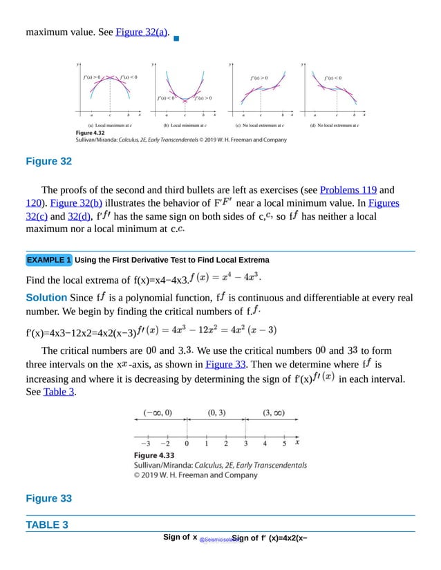
822. Interval Sign of x2 −3
3)
Conclusion
(−∞,0) Positive (+) Negative (−) Negative (−) f is decreasing
(0,3) Positive (+) Negative (−) Negative (−) f is decreasing
(3,∞) Positive (+) Positive (+) Positive (+) f is increasing
Using the First Derivative Test, f has neither a local maximum nor a local minimum at
0, and f has a local minimum at 3. The local minimum value is f(3)=−27. ▪
The graph of f is shown in Figure 34. Notice that the tangent line to the graph of f is
horizontal at the points (0,0) and (3,−27).
Figure 34 f(x)=x4−4x3
NOW WORK Problem 13.
EXAMPLE 2 Using the First Derivative Test to Find Local Extrema
Find the local extrema of f(x)=x2⁄3(x−5).
Solution The domain of f is all real numbers and f is continuous on its domain.
f′(x)=ddx[x2⁄3(x−5)]=x2⁄3+23⋅x−1⁄3(x−5)=x2⁄3+2(x−5)3x1⁄3=3x+2(x−5)3x1⁄3=5(x−2)3x1⁄3
@Seismicisolation
@Seismicisolation

823. Since f′(2)=0 and f′(0) does not exist, the critical numbers are 0 and 2.
Use the critical numbers 0 and 2 to form three intervals on the x -axis: (−∞,0 ),
(0,2 ), and (2,∞ ) as shown in Table 4.
TABLE 4
Interval
Sign of x
−2
Sign of
x1⁄3
Sign of f′(x)=5(x
−2)3x1⁄3
Conclusion
(−∞,0)
Negative
(−)
Negative
(−)
Positive (+) f is increasing
(0,2)
Negative
(−)
Positive
(+)
Negative (−) f is decreasing
(2,∞) Positive (+)
Positive
(+)
Positive (+) f is increasing
The sign of F′(x) on each interval tells us where f is increasing and decreasing.
By the First Derivative Test, f has a local maximum at 0 and a local minimum at 2;
f(0)=0 is the local maximum value and f(2)=−343 is the local
minimum value.
▪
Since F′(2)=0, the graph of f has a horizontal tangent line at the point
(2,−343). Since F′(0) does not exist and limx→0− F′(x)=∞
and limx→0+ F′(x)=−∞, the graph of f has a vertical
tangent line at the point (0,0) , a cusp. The graph of f is shown in Figure 35.
@Seismicisolation
@Seismicisolation

824. Figure 35 f(x)=x2⁄3(x−5)
NOW WORK Problems 21 and 51(a).
EXAMPLE 3 Obtaining Information About the Graph of f from the Graph of Its Derivative
A function f is continuous for all real numbers. Figure 36 shows the graph of its derivative
function F′.
a. Determine the critical numbers of f.
b. Where is f increasing?
c. Where is f decreasing?
d. At what numbers x, if any, does f have a local minimum?
e. At what numbers x, if any, does f have a local maximum?
@Seismicisolation
@Seismicisolation

825. Figure 36 y=f′(x)
Solution
a. The critical numbers of f occur where F′(x)=0 or where F′(x) does not
exist. Here F′ exists for all real numbers and the critical numbers of f are 0 and 2.
b. The function f is increasing where F′(x)>0; that is, where the graph of F′
is above the x -axis. This occurs for x>2. So f is increasing on the interval
(2,∞).
c. The function f is decreasing where F′(x)<0; that is, where the graph of F′
is below the x -axis. So f is decreasing on the intervals (−∞,0 ) and (0,2 ).
d. f is decreasing for x<2 and increasing for x>2, so by the First Derivative
Test, f has a local minimum at x=2.
e. f has no local maximum. (Do you see why?) There is no point (c,f(c)) on the
graph of f where f is increasing for x<c and decreasing for x>c. ▪
NOW WORK Problem 35.
2 Use the First Derivative Test with Rectilinear Motion
Increasing and decreasing functions can be used to investigate the motion of an object in
rectilinear motion. Suppose the signed distance s of an object from the origin at time t is
given by the position function s=f(t). We assume the motion is along a horizontal
@Seismicisolation
@Seismicisolation

826. line with the positive direction to the right. The velocity v of the object is v=dsdt.
If v=dsdt>0, the position s of the object is increasing with time t, and
the object moves to the right.
If v=dsdt<0, the position s of the object is decreasing with time t, and
the object moves to the left.
If v=dsdt=0, the object is at rest.
This information, along with the First Derivative Test, can be used to find the local
extreme values of s=f(t) and to determine at what times t the direction of the
motion of the object changes.
Similarly, if the acceleration of the object, a=dvdt>0, then the velocity of the
object is increasing, and if a=dvdt<0, then the velocity is decreasing. Again, this
information, along with the First Derivative Test, is used to find the local extreme values of
the velocity.
EXAMPLE 4 Using the First Derivative Test with Rectilinear Motion
An object moves along a horizontal line so that its signed distance s from the origin at time
t≥0, in seconds, is given by the position function
s=t3−9t2+15t+3
a. Determine the time intervals when the object is moving to the right.
b. Determine the time intervals when the object is moving to the left.
c. When does the object reverse direction?
d. Draw a figure that illustrates the motion of the object.
e. When is the velocity of the object increasing and when is it decreasing?
f. Draw a figure that illustrates the velocity of the object.
Solution To investigate the motion, we first find the velocity v.
v=dsdt= ddt (t3−9t2+15t+3)=3t2−18t+15=3(t2−6t+5)=3(t−1)(t−5)
@Seismicisolation
@Seismicisolation

827. The critical numbers are 1 and 5. We use the critical numbers to form three intervals on
the nonnegative t -axis: (0, 1), (1, 5), and (5, ∞ ) as shown in Table 5.
TABLE 5
Time Interval Sign of t−1 Sign of t−5 Velocity, v Position s Motion of the Object
(0,1) Negative (−) Negative (−) Positive (+) Increasing To the right
(1,5) Positive (+) Negative (−) Negative (−) Decreasing To the left
(5,∞) Positive (+) Positive (+) Positive (+) Increasing To the right
We use Table 5 to describe the motion of the object.
a. The object moves to the right for the first second and again after 5 s.
b. The object moves to the left on the interval (1,5).
c. The object reverses direction at t=1 and t=5.
d. Figure 37 illustrates the motion of the object.
Figure 37 s(t)=t3−9t2+15t+3
e. To determine when the velocity increases or decreases, we find the acceleration.
a=dvdt= ddt (3t2−18t+15)=6t−18=6(t−3)
Since a<0 on the interval (0,3), the velocity v decreases for the first 3 s. On
the interval (3,∞), a>0, so the velocity v increases from 3 s onward.
f. Figure 38 illustrates the velocity of the object.
▪
@Seismicisolation
@Seismicisolation

828. Figure 38 v(t)=3(t−1)(t−5)
An interesting phenomenon occurs during the first three seconds. The velocity of the
object is decreasing on the interval (0,3), as shown in Figure 38.
On the interval (0,3) the speed of the object is
|v(t)|=3|t2−6t+5|=3|(t−1)(t−5)|
If 0<t<1, |v(t)|=3(t2−6t+5) and d|v|dt=6(t−3)<0,
so the speed is decreasing.
If 1<t<3, |v(t)|=−3(t2−6t+5) and d|v|dt=−6(t−3)>0,
so the speed is increasing.
That is, the velocity of the object is decreasing from t=0 to t=3, but its speed is
decreasing from t=0 to t=1 and is increasing from t=1 to t=3.
NOW WORK Problem 29.
3 Determine the Concavity of a Function
Figure 39 shows the graphs of two familiar functions: y=x2, x≥0, and y=x.
Each graph starts at the origin, passes through the point (1,1), and is
increasing. But there is a noticeable difference in their shapes. The graph of y=x2
bends upward; it is concave up. The graph of y=x bends downward; it is concave
down.
@Seismicisolation
@Seismicisolation

829. Figure 39
Suppose we draw tangent lines to the graphs of y=x2 and y=x, as shown
in Figure 40. Notice that the graph of y=x2 lies above all its tangent lines, and moving
from left to right, the slopes of the tangent lines are increasing. That is, the derivative y
′=ddx x2 is an increasing function.
Figure 40 @Seismicisolation
@Seismicisolation

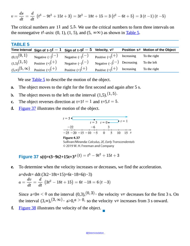
830. On the other hand, the graph of y=x lies below all its tangent lines, and moving
from left to right, the slopes of the tangent lines are decreasing. That is, the derivative y
′=ddxx is a decreasing function. This discussion leads to the following definition.
DEFINITION Concave Up; Concave Down
Let f be a function that is continuous on a closed interval [a,b] and differentiable on
the open interval (a,b).
f is concave up on (a,b) if the graph of f lies above each of its tangent lines
throughout (a,b).
f is concave down on (a,b) if the graph of f lies below each of its tangent lines
throughout (a,b).
We can formulate a test to determine where a function f is concave up or concave down,
provided f′′ exists. Since f′′ equals the rate of change of f′, it follows that if f′′(x)>0
on an open interval, then f′ is increasing on that interval, and if f′′(x)<0
on an open interval, then f′ is decreasing on that interval. As we observed in
Figure 40, when f′ is increasing, the graph is concave up, and when f′ is decreasing, the
graph is concave down. These observations lead to the Test for Concavity.
THEOREM Test for Concavity
Let f be a function that is continuous on a closed interval [a,b]. Suppose f′ and f′′
exist on the open interval (a,b).
If f′′(x)>0 on the interval (a,b), then f is concave up on (a,b).
If f′′(x)<0 on the interval (a,b), then f is concave down on (a,b).
NOTE When F′ and f″ both exist on an open interval (a,b ), the function f is called twice
differentiable on (a,b ).
Proof Suppose f′′(x)>0 on the interval (a,b), and c is any fixed number in
(a,b). An equation of the tangent line to f at the point (c,f(c)) is
y=f(c)+f′(c)(x−c) @Seismicisolation
@Seismicisolation

831. (1)
We need to show that the graph of f lies above each of its tangent lines for all x in (a,b).
That is, we need to show that
f(x)≥f(c)+f′(c)(x−c)for all x in (a,b)
If x=c, then f(x)=f(c) and we are finished.
If x≠c, then by applying the Mean Value Theorem to the function f, there is a
number x1 between c and x, for which
f′(x1)=f(x)−f(c)x−c
Now solve for f(x):
f(x)=f(c)+f′(x1)(x−c)
There are two possibilities: Either c<x1<x or x<x1<c.
Suppose c<x1<x. Since f′′(x)>0 on the interval (a,b), it
follows that f′ is increasing on (a,b). For x1>c, this means that f′(x1)>f′(c).
As a result, from (1), we have
f(x)>f(c)+f′(c)(x−c)
That is, the graph of f lies above each of its tangent lines to the right of c in (a,b).
Similarly, if x<x1<c, then f(x)>f(c)+f′(c)(x−c).
In all cases, f(x)≥f(c)+f′(c)(x−c) so f is concave up on (a,b).
The proof that if f′′(x)<0, then f is concave down is left as an exercise. See
Problem 121.
▪
EXAMPLE 5 Determining the Concavity of f(x)=ex
Show that f(x)=ex is concave up on its domain.
Solution The domain of f(x)=ex is all real numbers. The first and second
derivatives of f are
f′(x)=exf′′(x)=ex
Since f′′(x)>0 for all real numbers, by the Test for Concavity, f is concave up on
@Seismicisolation
@Seismicisolation

832. its domain.
▪
Figure 41 shows the graph of f(x)=ex and a selection of tangent lines to the
graph. Notice that for any x, the graph of f lies above its tangent lines.
Figure 41 f(x)=ex is concave up on its domain.
EXAMPLE 6 Finding Local Extrema and Determining Concavity
a. Find any local extrema of the function f(x)=x3−6x2+9x+30.
b. Determine where f(x)=x3−6x2+9x+30 is concave up and
where it is concave down.
Solution a. The first derivative of f is
f′(x)=3x2−12x+9=3(x−1)(x−3)
The function f is a polynomial, so its critical numbers occur when F′(x)=0.
So, 1 and 3 are critical numbers of f. Now
f′(x)=3(x−1)(x−3)>0 if x<1 or x>3.
f′(x)<0 if 1<x<3.
So f is increasing on (−∞,1) and on (3,∞); f is decreasing on (1,3).
At 1, f has a local maximum, and at 3, f has a local minimum. The local
maximum value is f(1)=34; the local minimum value is f(3)=30.
@Seismicisolation
@Seismicisolation

833. b. To determine concavity, we use the second derivative:
f′′(x)=6x−12=6(x−2)
Solve the inequalities f′′(x)<0 and f′′(x)>0 and use the Test for
Concavity.
f′′(x)<0if x<2,so f is concave down on (−∞,2)
f′′(x)>0if x>2,so f is concave up on (2,∞) ▪
Figure 42 shows the graph of f. The point (2,32) where the concavity of f
changes is of special importance and is called an inflection point.
Figure 42 f(x)=x3−6x2+9x+30
NOW WORK Problem 51(b).
4 Find Inflection Points
DEFINITION Inflection Point
Suppose f is a function that is differentiable on an open interval (a,b) containing c.
If the concavity of f changes at the point (c,f(c)), then (c,f(c)) is an
inflection point of f. @Seismicisolation
@Seismicisolation

834. If (c,f(c)) is an inflection point of f, then on one side of c the slopes of the
tangent lines are increasing (or decreasing), and on the other side of c the slopes of the
tangent lines are decreasing (or increasing). This means the derivative f′ must have a local
maximum or a local minimum at c. In either case, it follows that f′′(c)=0 or f′′(c)
does not exist.
THEOREM A Condition for an Inflection Point
Let f denote a function that is differentiable on an open interval (a,b) containing c.
If (c,f(c)) is an inflection point of f, then either f′′(c)=0 or f′′ does
not exist at c.
Notice the wording in the theorem. If you know that (c,f(c)) is an inflection point
of f, then the second derivative of f at c is 0 or does not exist. The converse is not
necessarily true. In other words, a number at which f′′(x)=0 or at which f′′ does
not exist will not always identify an inflection point.
Steps for Finding the Inflection Points of a Function f
Step 1 Find all numbers in the domain of f at which f′′(x)=0 or at which f′′
does not exist.
Step 2 Use the Test for Concavity to determine the concavity of f on both sides of each of
these numbers.
Step 3 If the concavity changes, there is an inflection point; otherwise, there is no
inflection point.
EXAMPLE 7 Finding Inflection Points
Find the inflection points of f(x)=x5⁄3.
Solution We follow the steps for finding an inflection point.
Step 1 The domain of f is all real numbers. The first and second derivatives of f are
f′(x)=53 x2⁄3f′′(x)=109x−1⁄3= 109x1⁄3
The second derivative of f does not exist when x=0. So, (0,0) is a
possible inflection point.
@Seismicisolation
@Seismicisolation

835. Step 2 Now use the Test for Concavity.
If x<0then f′′(x)<0 so f is concave down on (−∞,0).
If x>0then f′′(x)>0 so f is concave up on (0,∞).
Step 3 Since the concavity of f changes at 0, we conclude that (0,0) is an inflection
point of f. ▪
Figure 43 shows the graph of f with its inflection point (0,0 ) marked.
Figure 43 f(x)=x5⁄3
A change in concavity does not, of itself, guarantee an inflection point. For example,
Figure 44 shows the graph of f(x)=1x. The first and second derivatives are f′(x)=
−1x2 and f′′(x)=2x3. Then
f′′(x)=2x3<0if x<0andf′′(x)=2x3>0if x>0
@Seismicisolation
@Seismicisolation

836. Figure 44 f(x)=1x
So, f is concave down on (−∞,0) and concave up on (0,∞), yet f has no
inflection point at x=0 because 0 is not in the domain of f.
NOW WORK Problems 49 and 51(c).
EXAMPLE 8 Obtaining Information About the Graph of f from the Graphs of F′ and f″
A function f is continuous for all real numbers. The graphs of F′ and f″ are given in
Figure 45.
Figure 45
@Seismicisolation
@Seismicisolation

837. a. Determine the critical numbers of f.
b. Where is f increasing?
c. Where is f decreasing?
d. At what numbers x, if any, does f have a local minimum?
e. At what numbers x, if any, does f have a local maximum?
f. Where is f concave up?
g. Where is f concave down?
h. List any inflection points.
Solution
a. The critical numbers of f occur where F′(x)=0 or where F′ does not exist.
See Figure 45(a). Since F′ exists for all real numbers and since F′(0)=0 and
F′ 43=0, the only critical numbers are 0 and 43.
b. f is increasing where F′(x)>0; that is, where the graph of F′ is above the
x -axis. This occurs on the intervals (−∞,0) and 43,∞.
c. f is decreasing where F′(x)<0; that is, where the graph of F′ is below the
x -axis. This occurs on the interval 0,43.
d. Since f is decreasing for x<43 (F′(x)<0) and increasing for x>43 (F
′(x)>0), the function f has a local minimum at x=43.
e. Since f is increasing for x<0 (F′(x)>0) and decreasing for x>0
(F′(x)<0), the function f has local maximum at x=0.
f. f is concave up where f″(x)>0; that is, where the graph of f″ is above the
x -axis. See Figure 45(b). This occurs on the interval (1,∞).
g. f is concave down where f″(x)<0; that is, where the graph of f″ is below
the x -axis. This occurs on the intervals (−∞,0) and (0,1 ).
h. Inflection points occur at points on the graph of f where the concavity changes. The
concavity changes at x=1 so (1,f(1) ) is an inflection point.
▪
@Seismicisolation
@Seismicisolation

838. NOW WORK Problem 63.
5 Use the Second Derivative Test to Find Local Extrema
Suppose c is a critical number of f and f′(c)=0. This means that the graph of f
has a horizontal tangent line at the point (c,f(c)) . If f′′ exists on an open interval
containing c and f′′(c)>0, then the graph of f is concave up on the interval, as
shown in Figure 46(a). Intuitively, it would seem that f(c) is a local minimum value of f.
If, on the other hand, f′′(c)<0, the graph of f is concave down on the interval,
and f(c) would appear to be a local maximum value of f, as shown in Figure 46(b).
The next theorem, known as the Second Derivative Test, confirms our intuition.
Figure 46
THEOREM Second Derivative Test
Let f be a function for which f′ and f′′ exist on an open interval (a,b). Suppose
c lies in (a,b) and is a critical number of f:
If f′′(c)<0, then f(c) is a local maximum value.
If f′′(c)>0, then f(c) is a local minimum value.
Proof Suppose f′′(c)<0. Then
f′′(c)=limx→c f′(x)−f′(c)x−c<0 @Seismicisolation
@Seismicisolation

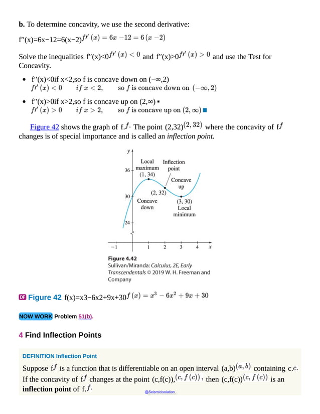
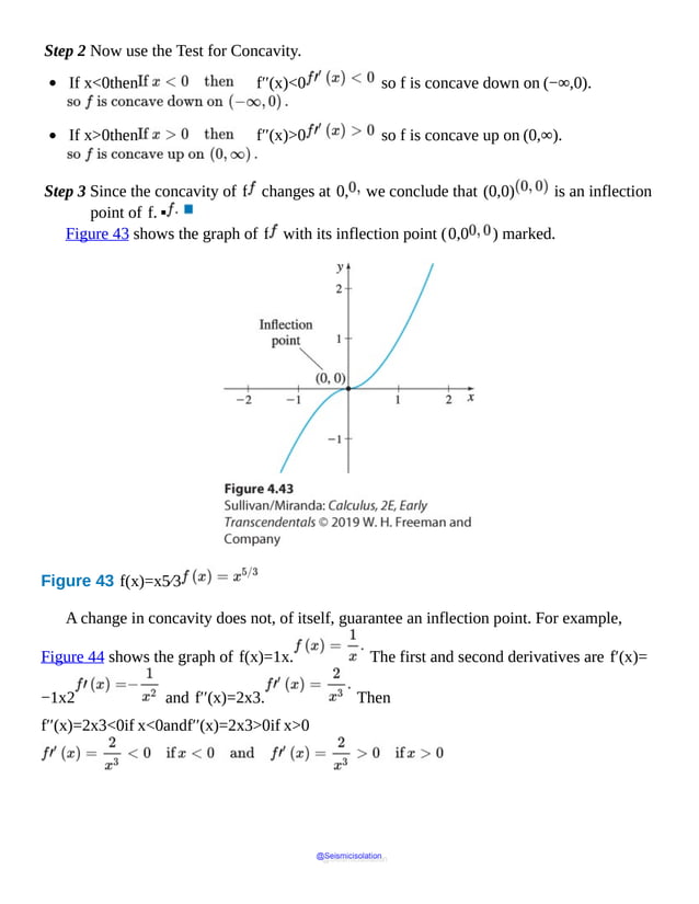
839. Now since limx→c f′(x)−f′(c)x−c<0, there is an open interval about c
for which
f′(x)−f′(c)x−c<0
everywhere in the interval, except possibly at c itself (refer to Example 7, p. 145, in Section
1.6). Since c is a critical number, f′(c)=0, so
f′(x)x−c<0
For x<c on this interval, f′(x)>0, and for x>c on this interval, f′(x)<0.
By the First Derivative Test, f(c) is a local maximum value.
▪
In Problem 122, you are asked to prove that if f′′(c)>0, then f(c) is a local
minimum value.
EXAMPLE 9 Using the Second Derivative Test to Identify Local Extrema
a. Determine where f(x)=x−2 cos x, 0 ≤x≤2π, is concave
up and concave down.
b. Find any inflection points.
c. Use the Second Derivative Test to identify any local extreme values.
Solution a. Since f is continuous on the closed interval [0,2π] and f′ and f′′
exist on the open interval 0,2π, we can use the Test for Concavity. The first and
second derivatives of f are
f′(x)=ddx (x−2 cos x)=1+2 sin xandf′′(x)=ddx (1+2 sin x)=2 cos x
To determine concavity, we solve the inequalities f′′(x)<0 and f′′(x)>0.
Since f′′(x)=2 cos x, we have
f′′(x)>0 when 0<x<π2 and 3π2<x<2π
f′′(x)<0 when π2<x<3π2
@Seismicisolation
@Seismicisolation

840. The function f is concave up on the intervals 0,π2 and 3π2,2π, and f is
concave down on the interval π2,3π2.
b. The concavity of f changes at π2 and 3π2, so the points π2,π2 and
3π2,3π2 are inflection points of f.
c. We find the critical numbers by solving the equation f′(x)=0.
1+2 sin x=00≤x≤2πsin x=−12x=7π6 or x=11π6
Using the Second Derivative Test, we get
f′′7π6=2 cos 7π6=−3<0
and
f′′11π6=2 cos 11π6=3>0
So,
f 7π6=7π6−2 cos 7π6=7π6+3≈5.397
is a local maximum value, and
f 11π6=11π6−2 cos 11π6=11π6−3≈4.028
is a local minimum value.
▪
See Figure 47 for the graph of f.
@Seismicisolation
@Seismicisolation

841. Figure 47 y=x−2 cos x, 0≤x≤2π
Sometimes the Second Derivative Test cannot be used, and sometimes it gives no
information.
If the second derivative of the function does not exist at a critical number, the Second
Derivative Test cannot be used.
If the second derivative exists at a critical number, but equals 0 there, the Second
Derivative Test gives no information.
In these situations, the First Derivative Test must be used to identify local extreme
points.
An example is the function f(x)=x4. Both f′(x)=4x3 and f′
′(x)=12x2 exist for all real numbers. Since f′(0)=0, 0 is a critical
number of f. But f′′(0)=0, so the Second Derivative Test gives no information
about the behavior of f at 0.
NOW WORK Problem 59.
Application: The Logistic Function in Business
EXAMPLE 10 Analyzing Monthly Sales
@Seismicisolation
@Seismicisolation

842. Unit monthly sales R of a new product over a period of time are expected to follow the
logistic function
R=R(t)=20,0001+50e−t−20,00051 t≥0
where t is measured in months.
a. When are the monthly sales increasing? When are they decreasing?
b. Find the rate of change of sales.
c. When is the rate of change of sales R′ increasing? When is it decreasing?
d. When is the rate of change of sales a maximum?
e. Find any inflection points of R.
f. Interpret the result found in (e) in the context of the problem.
Solution a. We find R′(t) and use the Increasing/Decreasing Function Test.
R′(t)=ddt 20,0001+50e−t−20,00051=20,000⋅50e−t(1+50e−t)2=1,000,000e−t(1+50e−t)2
Since e−t>0 for all t≥0, then R′(t)>0 for t≥0. The sales
function R is an increasing function. So, monthly sales are always increasing.
b. The rate of change of sales is given by the derivative R′(t)=1,000,000e−t(1+50e−t)2,
t≥0.
c. Using the Increasing/Decreasing Function Test with R′, the rate of change of sales R′
is increasing when its derivative R′′(t)>0; R′(t) is decreasing when R′′(t)
<0.
R′′(t)=ddt R′(t)=1,000,000[−e−t(1+50e−t)2+100e−2t(1+50e−t)(1+50e−t)4]=1,000,000e
−t[−1−50e−t+100e−t(1+50e−t)3]=1,000,000e−t(1+50e−t)3(50e−t−1)
Since e−t>0 for all t, the sign of R′′ depends on the sign of 50e−t−1.
@Seismicisolation
@Seismicisolation

843. 50e−t−1>0 50e−t−1<050e−t>1 50e−t<150>et 50<ett<ln 50t>ln 50
Since R′′(t)>0 for t<ln 50≈3.912 and R′′(t)<0 for
t>ln 50≈3.912, the rate of change of sales is increasing for the first 3.9
months and is decreasing from 3.9 months on.
d. The critical number of R′ is ln 50≈3.912. Using the First Derivative Test,
the rate of change of sales is a maximum about 3.9 months after the product is introduced.
e. Since R′′(t)>0 for t<ln 50 and R′′(t)<0 for t>ln 50,
the point (ln 50,9608) is the inflection point of R.
f. The sales function R is an increasing function, but at the inflection point (ln 50,9608)
the rate of change in sales begins to decrease.
▪
See Figure 48 for the graphs of R and R′.
Figure 48
NOW WORK Problem 93.
@Seismicisolation
@Seismicisolation

844. 4.4 Assess Your Understanding
Concepts and Vocabulary
1. True or False If a function f is continuous on the interval [a,b], differentiable on
the interval (a,b), and changes from an increasing function to a decreasing
function at the point (c,f(c)), then (c,f(c)) is an inflection point of f.
2. True or False Suppose c is a critical number of f and (a,b) is an open interval
containing c. If f′(x) is positive on both sides of c, then f(c) is a local
maximum value .
3. Multiple Choice Suppose a function f is continuous on a closed interval [a,b] and
differentiable on the open interval (a,b). If the graph of f lies above each of its
tangent lines on the interval (a,b), then on (a,b) f is
[a. concave up
b. concave down
c. neither].
4. Multiple Choice If the acceleration of an object in rectilinear motion is negative, then
the velocity of the object is
[a. increasing
b. decreasing
c. neither].
5. Multiple Choice Suppose f is a function that is differentiable on an open interval
containing c and the concavity of f changes at the point (c,f(c)). Then the
point (c,f(c)) on the graph of f is a(n)
[a. inflection point
b. critical point
c. both
d. neither].
6. Multiple Choice Suppose a function f is continuous on a closed interval [a,b] and
both f′ and f′′ exist on the open interval (a,b). If f′′(x)>0 on the
interval (a,b), then on (a,b) f is
@Seismicisolation
@Seismicisolation

845. [a. increasing
b. decreasing
c. concave up
d. concave down].
7. True or False Suppose f is a function for which f′ and f′′ exist on an open
interval (a,b) and suppose c, a<c<b, is a critical number of f. If f′
′(c)=0, then the Second Derivative Test cannot be used to determine if there
is a local extremum at c.
8. True or False Suppose a function f is differentiable on the open interval (a,b). If
either f′′(c)=0 or f′′ does not exist at the number c in (a,b), then
(c,f(c)) is an inflection point of f.
Skill Building
In Problems 9–12, the graph of a function f is given.
a. Identify the points where each function has a local maximum value, a local minimum
value, or an inflection point.
b. Identify the intervals on which each function is increasing, decreasing, concave up, or
concave down.
9.
10.
@Seismicisolation
@Seismicisolation

846. 11.
12.
@Seismicisolation
@Seismicisolation

847. In Problems 13–26, for each function:
a. Find the critical numbers.
b. Use the First Derivative Test to find any local extrema.
13. f(x)=x3−6x2+2
14. f(x)=x3+6x2+12x+1
15. f(x)=3x4−4x3
16. h(x)=x4+2x3−3
17. f(x)=(5−2x)ex
18. f(x)=(x−8)ex
19. f(x)=x2⁄3+x1⁄3
20. f(x)=12 x2⁄3−x1⁄3
21. g(x)=x2⁄3(x2−4)
22. f(x)=x1⁄3(x2−9)
23. f(x)=ln xx3
24. h(x)=ln xx3
@Seismicisolation
@Seismicisolation

848. 25. f(θ)=sin θ−2 cos θ
26. f(x)=x+2 sin x
In Problems 27–34, an object in rectilinear motion moves along a horizontal line with the
positive direction to the right. The position s of the object from the origin at time t≥0 (in
seconds) is given by the function s=s(t).
a. Determine the intervals during which the object moves to the right and the intervals
during which it moves to the left.
b. When does the object reverse direction?
c. When is the velocity of the object increasing and when is it decreasing?
d. Draw a figure to illustrate the motion of the object.
e. Draw a figure to illustrate the velocity of the object.
27. s=t2−2t+3
28. s=2t2+8t−7
29. s=2t3+6t2−18t+1
30. s=3t4−16t3+24t2
31. s=2t−6t, t>0
32. s=3t−1t, t>0
33. s=2 sin (3t),0≤t≤2π3
34. s=3 cos (πt),0≤t≤2
In Problems 35–38, the function f is continuous for all real numbers and the graph of its
derivative function f′ is given.
a. Determine the critical numbers of f.
b. Where is f increasing?
c. Where is f decreasing?
d. At what numbers x, if any, does f have a local minimum?
e. At what numbers x, if any, does f have a local maximum?
35.
@Seismicisolation
@Seismicisolation

849. 36.
37.
@Seismicisolation
@Seismicisolation

850. 38.
In Problems 39–62:
a. Find the local extrema of f.
b. Determine the intervals on which f is concave up and on which it is concave down.
c. Find any points of inflection.
39. f(x)=2x3−6x2+6x−3
40. f(x)=2x3+9x2+12x−4
41. f(x)=x4−4x
42. f(x)=x4+4x
@Seismicisolation
@Seismicisolation

851. 43. f(x)=5x4−x5
44. f(x)=4x6+6x4
45. f(x)=3x5−20x3
46. f(x)=3x5+5x3
47. f(x)=x2ex
48. f(x)=x3ex
49. f(x)=6x4⁄3−3x1⁄3
50. f(x)=x2⁄3−x1⁄3
51. f(x)=x2⁄3(x2−8)
52. f(x)=x1⁄3(x2−2)
53. f(x)=x2−ln x
54. f(x)=ln x−x
55. f(x)=x(1+x2)5⁄2
56. f(x)=x1+x
57. f(x)=x21−x2
58. f(x)=x1−x
59. f(x)=x−2 sin x, 0≤x≤2π
60. f(x)=2 cos2 x−sin2 x, 0≤x≤2π
61. f(x)=cosh x
62. f(x)=sinh x
In Problems 63–66, the function f is continuous for all real numbers and the graphs of F′
and f″ are given.
a. Determine the critical numbers of f.
b. Where is f increasing?
@Seismicisolation
@Seismicisolation

852. c. Where is f decreasing?
d. At what numbers x, if any, does f have a local minimum?
e. At what numbers x, if any, does f have a local maximum?
f. Where is f concave up?
g. Where is f concave down?
h. List any inflection points.
63.
64.
65.
@Seismicisolation
@Seismicisolation

853. 66.
In Problems 67–74, find the local extrema of each function f by:
a. Using the First Derivative Test.
b. Using the Second Derivative Test.
c. Discuss which of the two tests you found easier.
67. f(x)=−2x3+15x2−36x+7
68. f(x)=x3+10x2+25x−25
69. f(x)=x4−8x2−5
70. f(x)=x4+2x2+2
71. f(x)=3x5+5x4+1
72. f(x)=60x5+20x3
@Seismicisolation
@Seismicisolation

854. 73. f(x)=(x−3)2ex
74. f(x)=(x+1)2e−x
Applications and Extensions
In Problems 75–86, sketch the graph of a continuous function f that has the given properties.
Answers will vary.
75. f is concave up on (−∞,∞), increasing on (−∞,0), decreasing on
(0,∞), and f(0)=1.
76. f is concave up on (−∞,0), concave down on (0,∞), decreasing on
(−∞,0), increasing on (0,∞), and f(0)=1.
77. f is concave down on (−∞,1), concave up on (1,∞), decreasing on
(−∞,0), increasing on (0,∞), f(0)=1, and f(1)=2.
78. f is concave down on (−∞,0), concave up on (0,∞), increasing on
(−∞,∞), and f(0)=1 and f(1)=2.
79. f′(x)>0 if x<0 ; f′(x)<0 if x>0 ; f′′(x)>0 if
x<0 ; f′′(x)>0 if x>0 and f(0)=1.
80. f′(x)>0 if x<0 ; f′(x)<0 if x>0 ; f′′(x)>0 if
x<0 ; f′′(x)<0 if x>0 and f(0)=1.
81. f′′(0)=0 ; f′(0)=0 ; f′′(x)>0 if x<0 ; f′′(x)>0
if x>0 and f(0)=1.
82. f′′(0)=0 ; f′(x)>0 if x≠0 ; f′′(x)<0 if x<0 ; f′
′(x)>0 if x>0 and f(0)=1.
83. f′(0)=0 ; f′(x)<0 if x≠0 ; f′′(x)>0 if x<0 ; f′
′(x)<0 if x>0 ; f(0)=1.
84. f′′(0)=0 ; f′(0)=12 ; f′′(x)>0 if x<0 ; f′′(x)<0
if x>0 and f(0)=1.
85. f′(0) does not exist; f′′(x)>0 if x<0 ; f′′(x)>0 if x>0
and f(0)=1.
86. f′(0) does not exist; f′′(x)<0 if x<0 ; f′′(x)>0 if x>0
@Seismicisolation
@Seismicisolation

855. and f(0)=1.
In Problems 87–90, for each function:
a. Determine the intervals on which f is concave up and on which it is concave down.
b. Find any points of inflection.
c. Graph f and describe the behavior of f at each inflection point.
87. f(x)=e−(x−2)2
88. f(x)=x25−x
89. f(x)=2−x2x2−2x+1
90. f(x)=3xx2+3x+5
91. Inflection Point For the function f(x)=ax3+bx2, find a and b so
that the point (1,6) is an inflection point of f.
92. Inflection Point For the cubic polynomial function f(x)=ax3+bx2+cx+d,
find a, b, c, and d so that 0 is a critical number,
f(0)=4, and the point (1, −2) is an inflection point of f.
93. Public Health In a town of 50,000 people, the number of people at time t who
have influenza is N(t)=10,0001+9999e−t, where t is measured in
days. Note that the flu is spread by the one person who has it at t=0.
a. Find the rate of change of the number of infected people.
b. When is N′ increasing? When is it decreasing?
c. When is the rate of change of the number of infected people a maximum?
d. Find any inflection points of N.
e. Interpret the result found in (d) in the context of the problem.
94. Business The profit P (in millions of dollars) generated by introducing a new
technology is expected to follow the logistic function P(t)=3001+50e−0.2t,
where t is the number of years after its release.
a. When is annual profit increasing? When is it decreasing?
b. Find the rate of change in profit.
@Seismicisolation
@Seismicisolation

856. c. When is the rate of change in profit increasing? When is it decreasing?
d. When is the rate of change in profit a maximum?
e. Find any inflection points of P.
f. Interpret the result found in (e) in the context of the problem.
95. Population Model The following data represent the population of the United States:
Year Population Year Population
1900 76,212,168 1960 179,323,175
1910 92,228,486 1970 203,302,031
1920 106,021,537 1980 226,542,203
1930 123,202,624 1990 248,709,873
1940 132,164,569 2000 281,421,906
1950 151,325,798 2010 308,745,538
Source: U.S. Census Bureau.
An ecologist finds the data fit the logistic function
P(t)=762,176,717.81+8.743e−0.0162t.
a. Draw a scatterplot of the data using the years since 1900 as the independent
variable and population as the dependent variable.
b. Verify that P is the logistic function of best fit.
c. Find the rate of change in population.
d. When is P′ increasing? When is it decreasing?
e. When is the rate of change in population a maximum?
f. Find any inflection points of P.
g. Interpret the result found in (f) in the context of the problem.
96. Biology The amount of yeast biomass in a culture after t hours is given in the table
below.
Time
(in
hours)
Yeast Biomass
Time (in
hours)
Yeast Biomass
Time (in
hours)
Yeast Biomass
0 9.6 7 257.3 13 629.4
1 18.3 8 350.7 14 640.8
2 29.0 9 441.0 15 651.1
3 47.2 10 513.3 16 655.9
4 71.1 11 559.7 17 659.6
5 119.1 12 594.8 18 661.8
6 174.6 @Seismicisolation
@Seismicisolation

857. Source: Tor Carlson, Uber Geschwindigkeit und Grosse der Hefevermehrung in Wurrze,
Biochemische Zeitschrift, Bd. 57, 1913, pp. 313–334.
The logistic function y=663.01+71.6e−0.5470t, where t is time,
models the data.
a. Draw a scatterplot of the data using time t as the independent variable.
b. Verify that y is the logistic function of best fit.
c. Find the rate of change in biomass.
d. When is y′ increasing? When is it decreasing?
e. When is the rate of change in the biomass a maximum?
f. Find any inflection points of y.
g. Interpret the result found in (f) in the context of the problem.
97. U.S. Budget The United States budget documents the amount of money (revenue) the
federal government takes in (through taxes, for example) and the amount (expenses) it
pays out (for social programs, defense, etc.). When revenue exceeds expenses, we say
there is a budget surplus, and when expenses exceed revenue, there is a budget deficit.
The function
B=B(t)=−12.8t3+163.4t2−614.0t+390.6
where 0≤t≤12 approximates revenue minus expenses for the years 2000 to
2012, with t=0 representing the year 2000 and B in billions of dollars.
a. Find all the local extrema of B. (Round the answers to two decimal places.)
b. Do the local extreme values represent a budget surplus or a budget deficit?
c. Find the intervals on which B is concave up or concave down. Identify any
inflection points of B.
d. What does the concavity on either side of the inflection point(s) indicate about the
rate of change of the budget? Is it increasing at an increasing rate? Increasing at a
decreasing rate?
e. Graph the function B. Given that the budget for 2015 was 3.9 trillion dollars,
does B seem to be an accurate predictor for the budget for the years 2015 and
beyond?
98. If f(x)=ax3+bx2+cx+d, a≠0, how does the quantity
b2−3ac determine the number of potential local extrema?
99. If f(x)=ax3+bx2+cx+d, a≠0, find a, b, c, and d
@Seismicisolation
@Seismicisolation

858. so that f has a local minimum at 0, a local maximum at 4, and the graph
contains the points (0,5) and (4,33).
100. Find the local minimum of the function
f(x)=2x+81−x,0<x<1.
101. Find the local extrema and the inflection points of y=3 sin x+cos x,
0≤x≤2π.
102. If x>0 and n>1, can the expression xn−n(x−1)−1 ever
be negative?
103. Why must the First Derivative Test be used to find the local extreme values of the
function f(x)=x2⁄3?
104. Put It Together Which of the following is true of the function
f(x)=x2+e−2x
a. f is increasing
b. f is decreasing
c. f is discontinuous at 0
d. f is concave up
e. f is concave down
105. Put It Together If a function f is continuous for all x and if f has a local
maximum at (−1,4) and a local minimum at (3, −2), which of the
following statements must be true?
a. The graph of f has an inflection point somewhere between x=−1 and x=3.
b. f′(−1)=0.
c. The graph of f has a horizontal asymptote.
d. The graph of f has a horizontal tangent line at x=3.
e. The graph of f intersects both axes.
106. Vertex of a Parabola If f(x)=ax2+bx+c, a≠0, prove that f
has a local maximum at −b2a if a<0 and has a local minimum at −b2a
if a>0.
107. Show that sin x≤x, 0≤x≤2π. (Hint: Let f(x)=x−sin x.
@Seismicisolation
@Seismicisolation

859. )
108. Show that 1−x22≤cos x, 0≤x≤2π. (Hint: Use the result
of Problem 107.)
109. Show that 2x>3−1x, for x>1.
110. Use calculus to show that x2−8x+21>0 for all x.
111. Use calculus to show that 3x4−4x3−12x2+40>0 for all x.
112. Show that the function f(x)=ax2+bx+c, a≠0, has no
inflection points. For what values of a is f concave up? For what values of a is f
concave down?
113. Show that every polynomial function of degree 3 f(x)=ax3+bx2+cx+d
has exactly one inflection point.
114. Prove that a polynomial of degree n≥ 3 has at most (n−1) critical
numbers and at most (n−2) inflection points.
115. Show that the function f(x)=(x−a)n, a a constant, has exactly one
inflection point if n≥3 is an odd integer.
116. Show that the function f(x)=(x−a)n, a a constant, has no inflection
point if n≥2 is an even integer.
117. Show that the function f(x)=ax+bax+d has no critical points and no
inflection points.
118.
a. Show that the second derivative of the logistic function
f(t)=c1+ae−bta>0,c>0
is
f″(t)=ab2ce−bt(ae−bt−1)
b. Show that the logistic function f has an inflection point at
ln ab,c2
119. First Derivative Test Proof Let f be a function that is continuous on an interval I.
@Seismicisolation
@Seismicisolation

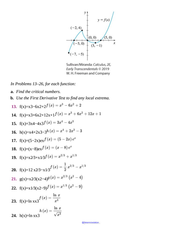
860. Suppose c is a critical number of f and (a,b) is an open interval in I
containing c. Prove that if f′(x)<0 for a<x<c and f′(x)>0
for c<x<b, then f(c) is a local minimum value.
120. First Derivative Test Proof Let f be a function that is continuous on an interval I.
Suppose c is a critical number of f and (a,b) is an open interval in I
containing c. Prove that if f′(x) has the same sign on both sides of c, then
f(c) is neither a local maximum value nor a local minimum value.
121. Test of Concavity Proof Let f be a function that is continuous on a closed interval
[a,b]. Suppose f′ and f′′ exist on the open interval (a,b). Prove that if
f′′(x)<0 on the interval (a,b), then f is concave down on (a,b).
122. Second Derivative Test Proof Let f be a function for which f′ and f′′ exist on an
open interval (a,b). Suppose c lies in (a,b) and is a critical number of f.
Prove that if f′′(c)>0, then f(c) is a local minimum value.
Challenge Problems
123. Find the inflection point of y=x+1 tan−1x.
124. Bernoulli’s Inequality Prove (1+x)n>1+nx for x>−1, x≠
0, and n>1. (Hint: Let f(x)=(1+x)n−(1+nx). )
1. = NOW WORK problem
= Graphing technology recommended
= Computer Algebra System recommended
@Seismicisolation
@Seismicisolation

861. (1)
4.5 Indeterminate Forms and L’Hôpital’s Rule
OBJECTIVES When you finish this section, you should be able to:
1 Identify indeterminate forms of the type 00 and ∞∞
2 Use L’Hôpital’s Rule to find a limit
3 Find the limit of an indeterminate form of the type 0⋅∞, ∞−∞, 00, 1∞, or ∞0
In this section, we reexamine the limit of a quotient and explore what we can do when
previous strategies cannot be used. The discussion here will prove helpful in the next section.
NEED TO REVIEW? The limit of a quotient is discussed in Section 1.2, pp. 96–98.
1 Identify Indeterminate Forms of the Type 00 and ∞∞
To find limx→c f(x)g(x) we usually first try to use the Limit of a Quotient:
limx→c f(x)g(x)=limx→c f(x)limx→c g(x)
But the quotient property cannot always be used. For example, to find limx→2 x2−4x−2,
we cannot use (1), since the numerator and the denominator each approach 0
(resulting in the form 00). Instead, we use algebra and obtain
limx→2 x2−4x−2=limx→2 (x−2)(x+2)x−2=limx→2 (x+2)=4
To find limx→∞ 3x−2x2+5, we cannot use equation (1), since the
numerator and the denominator each become unbounded (resulting in the form ∞∞ ).
Instead, we use the end behavior of polynomial functions. Then
@Seismicisolation
@Seismicisolation

862. limx→∞ 3x−2x2+5=limx→∞ 3x=0
NEED TO REVIEW? Limits at infinity and infinite limits are discussed in Section 1.5, pp. 128–135.
As a third example, to find limx→0 sin xx, we cannot use equation (1) since it
leads to the form 00. Instead, we use a geometric argument (the Squeeze Theorem) to
show that
limx→0 sin xx=1
When limx→c f(x)g(x)=limx→c f(x)limx→c g(x) leads to the
form 00 or ∞∞, we say that fg is an indeterminate form at c. Then depending on
the functions f and g, limx→c f(x)g(x), if it exists, could equal 0, ∞, or
some nonzero real number.
NOTE The word ”indeterminate” conveys the idea that the limit cannot be found without additional work.
DEFINITION Indeterminate Form at c of the Type 00 or the Type ∞∞
If the functions f and g are each defined in an open interval containing the number c,
except possibly at c, then the quotient f(x)g(x) is called an indeterminate form at
c of the type 00 if
limx→c f(x)=0 and limx→c g(x)=0
and an indeterminate form at c of the type ∞∞ if
limx→c f(x)=±∞ and limx→c g(x)=±∞
@Seismicisolation
@Seismicisolation

863. These definitions also hold for limits at infinity.
NOTE 00 and ∞∞ are symbols used to denote an indeterminate form.
EXAMPLE 1 Identifying an Indeterminate Form of the Type 00 or ∞∞
a. cos (3x)−12x is an indeterminate form at 0 of the type 00 since
limx→0 [cos (3x)−1]=0andlimx→0 (2x)=0
b. x−1x2+2x−3 is an indeterminate form at 1 of the type 00 since
limx→1 (x−1)=0 andlimx→1 (x2+2x−3)=0
c. x2−2x−3 is not an indeterminate form at 3 of the type 00 since
limx→3 (x2−2)≠0.
d. x2ex is an indeterminate form at ∞ of the type ∞∞ since
limx→∞ x2=∞andlimx→∞ ex=∞ ▪
NOW WORK Problem 7.
2 Use L’Hôpital’s Rule to Find a Limit
A theorem, named after the French mathematician Guillaume François de L’Hôpital
(pronounced “low-pee-tal”), provides a method for finding the limit of an indeterminate
form.
THEOREM L’Hôpital’s Rule
Suppose the functions f and g are differentiable on an open interval I containing the
number c, except possibly at c, and g′(x)≠0 for all x≠c in I. Let L
@Seismicisolation
@Seismicisolation

864. denote either a real number or ±∞, and suppose f(x)g(x) is an indeterminate
form at c of the type 00 or ∞∞. If limx→c f′(x)g′(x)=L, then
limx→c f(x)g(x)=L.
L’Hôpital’s Rule is also valid for limits at infinity and one-sided limits. A partial proof of
L’Hôpital’s Rule is given in Appendix B. A limited proof is given here that assumes f′ and
g′ are continuous at c and g′(c)≠0.
Proof Suppose limx→c f(x)=0 and limx→c g(x)=0 Then f(c)=0
and g(c)=0. Since both f′ and g′ are continuous at c and g′(c)≠0,
we have
matrix
Element
1
1
x
right
arrow
c
under
lim
start
frac
f
super
prime
▪
Steps for Finding a Limit Using L’Hôpital’s Rule
Step 1 Check that fg is an indeterminate form at c of the type 00 or ∞∞. If it is
not, do not use L’Hôpital’s Rule.
Step 2 Differentiate f and g separately.
Step 3 Find limx→c f′(x)g′(x). This limit is equal to limx→c f(x)g(x),
provided the limit is a number or ∞ or −∞.
@Seismicisolation
@Seismicisolation

865. Step 4 If f′g′ is an indeterminate form at c, repeat the process.
IN WORDS If limx→c f(x)g(x) leads to 00 or ∞∞, L’Hôpital’s Rule states that the limit of the
quotient equals the limit of the quotient of their derivatives.
ORIGINS Guillaume François de L’Hôpital (1661–1704) was a French nobleman. When he was 30, he hired
Johann Bernoulli to tutor him in calculus. Several years later, he entered into a deal with Bernoulli. L’Hôpital
paid Bernoulli an annual sum for Bernoulli to share his mathematical discoveries with him but no one else. In
1696 L’Hôpital published the first textbook on differential calculus. It was immensely popular, the last edition
being published in 1781 (seventy-seven years after L’Hôpital’s death). The book included the rule we study
here. After L’Hôpital’s death, Johann Bernoulli made his deal with L’Hôpital public and claimed that L’Hôpital’s
textbook was his own material. His position was dismissed because he often made such claims. However, in
1921, the manuscripts of Bernoulli’s lectures to L’Hôpital were found, showing L’Hôpital’s calculus book was
indeed largely Johann Bernoulli’s work.
EXAMPLE 2 Using L’Hôpital’s Rule to Find a Limit
Find limx→0 tan x6x.
Solution We follow the steps for finding a limit using L’Hôpital’s Rule.
Step 1 Since limx→0 tan x=0 and limx→0 (6x)=0, the quotient
tan x6x is an indeterminate form at 0 of the type 00.
Step 2 ddx tan x=sec2x and ddx 6x=6.
@Seismicisolation
@Seismicisolation

866. Step 3 limx→0 ddx tan xddx 6x= limx→0 sec2x6=16. It
follows from L’Hôpital’s Rule that limx→0 tan x6x=16. ▪
In the solution of Example 2, we were careful to determine that the limit of the ratio of
the derivatives, that is, limx→0 sec2x6, existed or became infinite before using
L’Hôpital’s Rule. However, the usual practice is to combine Step 2 and Step 3 as follows:
limx→0 tan x6x=limx→0 ddx tan xddx (6x)=limx→0 sec2x6=16
CAUTION When using L’Hôpital’s Rule, we find the derivative of the numerator and the derivative of the
denominator separately. Be sure not to find the derivative of the quotient. Also, using L’Hôpital’s Rule to find a
limit of an expression that is not an indeterminate form may result in an incorrect answer.
NOW WORK Problem 29.
At times, it is necessary to use L’Hôpital’s Rule more than once.
EXAMPLE 3 Using L’Hôpital’s Rule to Find a Limit
Find limx→0 sin x−xx2.
Solution Use the steps for finding a limit using L’Hôpital’s Rule.
Step 1 Since limx→0 sinx−x=0 and limx→0 x2=0, the
expression sin x−xx2 is an indeterminate form at 0 of the type 00.
Steps 2 and 3 Use L’Hôpital’s Rule.
@Seismicisolation
@Seismicisolation

867. Step 4 Since limx→0 (cos x−1)=0 and limx→0 x=0, the
expression cos x−1x is an indeterminate form at 0 of the type 00. So,
use L’Hôpital’s Rule again.
▪
NOW WORK Problem 39.
EXAMPLE 4 Using L’Hôpital’s Rule to Find a Limit at Infinity
Find:
a. limx→∞ ln xx
b. limx→∞ xex
c. limx→∞ exx
Solution a. Since limx→∞ln x=∞ and limx→∞ x=∞, ln xx
is an indeterminate form at ∞ of the type ∞∞. Using L’Hôpital’s Rule,
b. limx→∞ x=∞ and limx→∞ ex=∞, so xex is an indeterminate
form at ∞ of the type ∞∞. Using L’Hôpital’s Rule,
@Seismicisolation
@Seismicisolation

868. c. From (b), we know that exx is an indeterminate form at ∞ of the type ∞∞. Using
L’Hôpital’s Rule,
▪
NOW WORK Problem 35.
The results from Example 4 tell us that y=x grows faster than y=ln x, and
that y=ex grows faster than y=x. In fact, these inequalities are true for all
positive powers of x. That is,
limx→∞ ln xxn=0limx→∞ xnex=0
for n≥1 an integer. You are asked to verify these results in Problems 95 and 96.
Sometimes simplifying first reduces the effort needed to find the limit.
EXAMPLE 5 Using L’Hôpital’s Rule to Find a Limit
Find limx→0 tan x−sin xx2 tan x.
Solution tan x−sin xx2 tan x is an indeterminate form at 0 of the type 00.
We simplify the expression before using L’Hôpital’s Rule. Then it is easier to find the limit.
tan x−sin xx2 tan x=sin xcos x−sin xx2⋅sin xcos x=sin x
−sin x cos xcos xx2 sin xcos x=sin x(1−cos x)x2 sin x=1−cos xx2
CAUTION Be sure to verify that a simplified form is an indeterminate form at c before using L’Hôpital’s Rule.
Since 1−cos xx2 is an indeterminate form at 0 of the type 00, we use
@Seismicisolation
@Seismicisolation

869. L’Hôpital’s Rule.
▪
Compare this solution to one that uses L’Hôpital’s Rule at the start.
In Example 6, we use L’Hôpital’s Rule to find a one-sided limit.
EXAMPLE 6 Using L’Hôpital’s Rule to Find a One-Sided Limit
Find limx→0+ cot xln x.
Solution Since limx→0+ cot x=∞ and limx→0+ln x=−∞,
cot xln x is an indeterminate form at 0+ of the type ∞∞. Using L’Hôpital’s
Rule,
▪
NOW WORK Problem 61.
3 Find the Limit of an Indeterminate Form of the Type 0⋅∞, ∞−∞,
00, 1∞, or ∞0
L’Hôpital’s Rule can only be used for indeterminate forms of the types 00 and ∞∞. We
need to rewrite indeterminate forms of the type 0⋅∞, ∞−∞, 00, 1∞, or
@Seismicisolation
@Seismicisolation

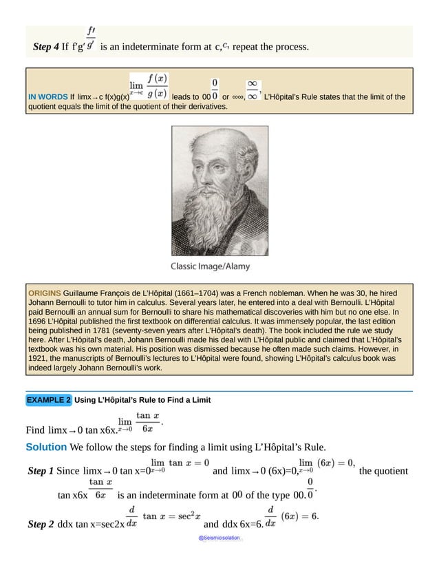
870. ∞0 in the form 00 or ∞∞ before using L’Hôpital’s Rule to find the limit.
Indeterminate Forms of the Type 0⋅∞
Suppose limx→c f(x)=0 and limx→c g(x)=0. Depending on the
functions f and g, limx→c [f(x)⋅g(x)], if it exists, could equal 0, ∞,
or some nonzero number. The product f⋅g is called an indeterminate form at c of the
type 0⋅∞.
To find limx→c (f⋅g), rewrite the product f⋅g as one of the following
quotients:
f⋅g=f1g orf⋅g=g1f
NOTE It might be tempting to argue that 0⋅∞ is 0, since “anything” times 0 is 0, but 0⋅∞ is
not a product of numbers. That is, 0⋅∞ is not “zero times infinity”; it symbolizes “a quantity tending to
zero” times “a quantity tending to infinity.”
The right side of the equation on the left is an indeterminate form at c of the type 00; the
right side of the equation on the right is of the type ∞∞. Then use L’Hôpital’s Rule with
one of these quotients, choosing the one for which the derivatives are easier to find. If the
first choice does not work, then try the other one.
EXAMPLE 7 Finding the Limit of an Indeterminate Form of the Type 0⋅∞
Find:
a. limx→0+ (x ln x)
b. limx→∞ x sin 1x
NOTE We choose to use ln x1x rather than x1ln x because it is easier to find the derivatives of
ln x and 1x than it is to find the derivatives of x and 1ln x.
@Seismicisolation
@Seismicisolation

871. Solution a. Since limx→0+ x=0 and limx→0+ln x=−∞, then
x ln x is an indeterminate form at 0+ of the type 0⋅∞. Change x ln x to
an indeterminate form of the type ∞∞ by writing x ln x=ln x1x. Then use
L’Hôpital’s Rule.
limx→0+ (x ln x)=limx→0+ ln x1x=limx→0+ ddx ln xddx 1x=limx→0+ 1x
− 1x2=limx→0+ (−x)=0
b. Since limx→∞ x=∞ and limx→∞ sin 1x=0, then x sin 1x
is an indeterminate form at ∞ of the type 0⋅∞. Change x sin 1x to
an indeterminate form of the type 00 by writing
▪
NOTE Notice in the solution to (b) that we did not need to use L’Hôpital’s Rule.
NOW WORK Problem 45.
Indeterminate Forms of the Type ∞−∞
Suppose limx→c f(x)=∞ and limx→c g(x)=∞. Then depending
on the functions f and g, limx→c [f(x)−g(x)], if it exists, could equal
0, ∞, or some nonzero number. In such instances the difference f(x)−g(x) is
called an indeterminate form at c of the type ∞−∞.
If the limit of a function results in the indeterminate form ∞−∞, it is generally
@Seismicisolation
@Seismicisolation

872. possible to rewrite the function as an indeterminate form of the type 00 or ∞∞ by using
algebra or trigonometry.
NOTE The indeterminate form of the type ∞−∞ is a convenient notation for any of the following: ∞−∞,
−∞−(−∞), ∞+(−∞). Note that ∞+∞=∞ and (−∞)+
(−∞)=−∞ are not indeterminate forms because there is no confusion about these
sums.
EXAMPLE 8 Finding the Limit of an Indeterminate Form of the Type ∞−∞
Find limx→0+ 1x−1sin x.
Solution Since limx→0+ 1x=∞ and limx→0+ 1sin x=∞, then
1x−1sin x is an indeterminate form at 0+ of the type ∞−∞. Rewrite the
difference as a single fraction.
limx→0+ 1x−1sin x=limx→0+ sin x−xx sin x
Then sin x−xx sin x is an indeterminate form at 0+ of the type 00. Now use
L’Hôpital’s Rule.
▪
NOW WORK Problem 47.
Indeterminate Forms of the Type 1∞, 00, or ∞0
@Seismicisolation
@Seismicisolation

873. A function of the form [f(x)]g(x) may result in an indeterminate form of the type
1∞, 00, or ∞0. To find the limit of such a function, we let y=[f(x)]g(x)
and take the natural logarithm of each side.
ln y=ln [f(x)]g(x)=g(x)ln f(x)
NEED TO REVIEW? Properties of logarithms are discussed in Appendix A.1, pp. A-10 to A-11.
The expression on the right will then be an indeterminate form of the type 0⋅∞ and we
find the limit using the method of Example 7.
Steps for Finding limx→c [f(x)]g(x) When [f(x)]g(x) Is an Indeterminate Form
at c of the Type 1∞ , 00 , or ∞0
Step 1 Let y=[f(x)]g(x) and take the natural logarithm of each side, obtaining
ln y=g(x)ln f(x).
Step 2 Find limx→c ln y.
Step 3 If limx→c ln y=L, then limx→c y=eL.
These steps also can be used for limits at infinity and for one-sided limits.
EXAMPLE 9 Finding the Limit of an Indeterminate Form of the Type 00
Find limx→0+ xx.
Solution The expression xx is an indeterminate form at 0+ of the type 00. Follow
the steps for finding limx→c [f(x)]g(x).
Step 1 Let y=xx. Then ln y=x ln x.
Step 2 limx→0+ln y=limx→0+(x ln x)=0 [from Example 7(a)].
Step 3 Since limx→0+ln y=0, limx→0+ y=e0=1. ▪
CAUTION Do not stop after finding limx→c ln y (=L). Remember, we want to find
@Seismicisolation
@Seismicisolation

874. limx→c y (=eL).
NOW WORK Problem 51.
EXAMPLE 10 Finding the Limit of an Indeterminate Form of the Type 1∞
Find limx→0+ (1+x)1⁄x.
Solution The expression (1+x)1⁄x is an indeterminate form at 0+ of the type 1∞.
Step 1 Let y=(1+x)1⁄x. Then ln y=1x ln(1+x).
Step 2
Step 3 Since limx→0+ln y=1, limx→0+ y=e1=e. ▪
NOW WORK Problem 85.
4.5 Assess Your Understanding
Concepts and Vocabulary
1. True or False f(x)g(x) is an indeterminate form at c of the type 00 if
limx→c f(x)g(x) does not exist.
2. True or False If f(x)g(x) is an indeterminate form at c of the type 00, then
L’Hôpital’s Rule states that limx→c f(x)g(x)=limx→c [ddxf(x)g(x)].
3. True or False 1x is an indeterminate form at 0.
@Seismicisolation
@Seismicisolation

875. 4. True or False x ln x is not an indeterminate form at 0+ because limx→0+ x=0
and limx→0+ln x=−∞, and 0⋅−∞=0.
5. In your own words, explain why ∞−∞ is an indeterminate form, but ∞+∞
is not an indeterminate form.
6. In your own words, explain why 0⋅∞≠0.
Skill Building
In Problems 7–26:
a. Determine whether each expression is an indeterminate form at c.
b. If it is, identify the type. If it is not an indeterminate form, state why.
7. 1−exx, c=0
8. 1−exx−1, c=0
9. exx, c=0
10. exx, c=∞
11. ln xx2, c=∞
12. ln(x+1)ex−1, c=0
13. sec xx, c=0
14. xsec x−1, c=0
15. sin x(1−cos x)x2, c=0
16. sin x−1cos x, c=π2
17. tan x−1sin (4x−π), c=π4
@Seismicisolation
@Seismicisolation

876. 18. ex−e−x1−cos x, c=0
19. x2e−x, c=∞
20. x cot x, c=0
21. csc x2−cot x2, c=0
22. xx−1+1ln x, c=1
23. 1x2sin x, c=0
24. (ex+x)1⁄x, c=0
25. (x2−1)x, c=0
26. (sin x)x, c=0
In Problems 27–42, identify each quotient as an indeterminate form of the type 00 or ∞∞.
Then find the limit.
27. limx→2 x2+x−6x2−3x+2
28. limx→1 2x3+5x2−4x−3x3+x2−10x+8
29. limx→1 ln xx2−1
30. limx→0 ln(1−x)ex−1
31. limx→0 ex−e−xsin x
32. limx→0 tan (2x)ln(1+x)
33. limx→1 sin (πx)x−1 @Seismicisolation
@Seismicisolation

877. 34. limx→π 1+cos xsin (2x)
35. limx→∞ x2ex
36. limx→∞ exx4
37. limx→∞ lnxex
38. limx→∞ x+lnxxlnx
39. limx→0 ex−1−sin x1−cos x
40. limx→0 ex−e−x−2 sin x3x3
41. limx→0 sin x−xx3
42. limx→0 x3cos x−1
In Problems 43–58, identify each expression as an indeterminate form of the type 0⋅∞,
∞−∞, 00, 1∞, or ∞0. Then find the limit.
43. limx→0+ (x2ln x)
44. limx→∞ (xe−x)
45. limx→∞ [x(e1⁄x−1)]
46. limx→π/2 [(1−sin x) tan x]
47. limx→π/2 (sec x−tan x)
48. limx→0 (cot x−1x)
49. limx→1 1ln x−xln x
@Seismicisolation
@Seismicisolation

878. 50. limx→0 1x−1ex−1
51. limx→0+ (2x)3x
52. limx→0+ xx2
53. limx→∞ (x+1)e−x
54. limx→∞ (1+x2)1⁄x
55. limx→0+ (csc x)sin x
56. limx→∞ x1⁄x
57. limx→π/2− (sin x)tan x
58. limx→0 (cos x)1⁄x
In Problems 59–90, find each limit.
59. limx→0+ cot xcot (2x)
60. limx→∞ ln(ln x)ln x
61. limx→1/2− ln(1−2x)tan (πx)
62. limx→1− ln(1−x)cot (πx)
63. limx→∞ x4+x3ex+1
64. limx→∞ x2+x−1ex+e−x
65. limx→0 xe4x−x1−cos (2x) @Seismicisolation
@Seismicisolation

879. 66. limx→0 x tan x1−cos x
67. limx→0 tan−1xx
68. limx→0 tan−1xsin−1x
69. limx→0 cos x−1 cos (2x)−1
70. limx→0 tan x−sin xx3
71. limx→0+ (x1⁄2 ln x)
72. limx→∞ [(x−1)e−x2]
73. limx→π/2 [tan x ln(sin x)]
74. limx→0+ [sin x ln(sin x)]
75. limx→0[csc x ln(x+1)]
76. limx→π/4− [(1−tan x)sec (2x)]
77. limx→a [(a2−x2)tan πx2a]
78. limx→1+ [(1−x) tan 12 πx ]
79. limx→1 1lnx−1x−1
80. limx→1 xx−1−1lnx
81. limx→π/2 x tan x−π2 sec x
82. limx→π (cotx−xcscx)
@Seismicisolation
@Seismicisolation

880. 83. limx→1− (1−x)tan (πx)
84. limx→0+ xx
85. limx→0 sin xx1⁄x
86. limx→∞ 1+5x+3x2x
87. limx→(π/2)− (tan x)cos x
88. limx→0+ (x2+x)−ln x
89. limx→0 (coshx)ex
90. limx→0+ (sinh x)x
Applications and Extensions
91. Wolf Population In 2014 there were 229 wolves in Wyoming outside of
Yellowstone National Park. Suppose the population w of wolves in the region at time
t follows the logistic growth curve
w=w(t)=KertK40+ert−1
where K=252, r=0.283, and t=0 represents the population in
the year 2000.
Source: Federal Wildlife Service
a. Find limt→∞ w(t).
b. Interpret the answer found in (a) in the context of the problem.
c. Use technology to graph w=w(t).
92. Skydiving The downward velocity v of a skydiver with nonlinear air resistance can be
modeled by
@Seismicisolation
@Seismicisolation

881. v=v(t)=−A+RA eBt+C−1eBt+C+1
where t is the time in seconds, and A,B,C, and R are positive constants with
R>1.
a. Find limt→∞ v(t).
b. Interpret the limit found in (a).
c. If the velocity v is measured in feet per second, reasonable values of the constants
are A=108.6, B=0.554, C=0.804, and R=2.62.
Graph the velocity of the skydiver with respect to time.
93. Electricity The equation governing the amount of current I (in amperes) in a simple
RL circuit consisting of a resistance R (in ohms), an inductance L (in henrys), and
an electromotive force E (in volts) is I=ER (1−e−Rt⁄L).
a. Find limx→∞ I(t) and limR→0+ I(t).
b. Interpret these limits.
94. Find limx→0 ax−bxx, where a≠1 and b≠1 are positive real
numbers.
95. Show that limx→∞ lnxxn=0, for n≥1 an integer.
96. Show that limx→∞ xnex=0 for n≥1 an integer.
97. Show that limx→0+(cos x+2 sin x)cot x=e2.
@Seismicisolation
@Seismicisolation

882. 98. Find limx→∞ P(x)ex, where P is a polynomial function.
99. Find limx→∞ln(x+1)−ln(x−1).
100. Show that limx→0+ e−1⁄x2x=0. Hint: Write e−1⁄x2x=1xe1⁄x2.
101. If n is an integer, show that limx→0+ e−1⁄x2xn=0.
102. Show that limx→∞xx=1.
103. Show that limx→∞1+axx=ea, a any real number.
104. Show that limx→∞x+ax−ax= e2a,a≠0.
105.
a. Show that the function below has a derivative at 0. What is f′(0)?
f(x)={e−1⁄x2ifx ≠ 00 if x = 0
b. Graph f.
106. If a,b≠0 and c>0 are real numbers, show that
limx→c xa−caxb−cb=ab ca−b.
107. Prove L’Hôpital’s rule when f(x)g(x) is an indeterminate form at −∞ of the
type 00.
Challenge Problems
108. Explain why L’Hôpital’s Rule does not apply to limx→0 x2sin 1xsin x.
@Seismicisolation
@Seismicisolation

883. 109. Find each limit:
a. limx→∞ 1+1x−x2
b. limx→∞ 1+lnaxx, a>1
c. limx→∞ 1+1xx2
d. limx→∞ 1+sin xxx
e. limx→∞ (ex)−1⁄ln x
f. limx→∞ [1ax]−1⁄x, 0<a<1
g. limx→∞ x1⁄x
h. limx→∞ (ax)1⁄x, a>1
i. limx→∞ [(2+sin x)x]1⁄x
j. limx→0+ x−1⁄ln x
110. Find constants A, B, C, and D so that
limx→0 sin (Ax)+Bx+Cx2+Dx3x5=415
111. A function f has derivatives of all orders.
a. Find limh→0 f(x+2h)−2 f(x+h)+f(x)h2.
b. Find limh→0 f(x+3h)−3 f(x+2h)+3 f(x+h)−f(x)h3.
c. Generalize parts (a) and (b).
112. The formulas in Problem 111 can be used to approximate derivatives. Approximate f
′(2), f′′(2), and f‴(2) from the table. The data are for f(x)=ln x.
@Seismicisolation
@Seismicisolation

884. Compare the exact values with your approximations.
x 2.0 2.1 2.2 2.3 2.4
f(x) 0.6931 0.7419 0.7885 0.8329 0.8755
113. Consider the function f(t,x)=xt+1−1t+1, where x>0 and t≠−1.
a. For x fixed at x0, show that limt→−1 f(t,x0)=lnx0.
b. For x fixed, define a function F (t,x), where x>0, that is
continuous so F (t,x)=f(t,x) for all t≠−1.
c. For t fixed, show that ddx F (t,x)=xt, for x>0 and all t.
Source: Michael W. Ecker (2012, September), Unifying Results via L’Hôpital’s Rule.
Journal of the American Mathematical Association of Two Year Colleges, 4(1) pp.
9–10.
1. = NOW WORK problem
= Graphing technology recommended
= Computer Algebra System recommended
@Seismicisolation
@Seismicisolation

885. 4.6 Using Calculus to Graph Functions
OBJECTIVES When you finish this section, you should be able to:
1 Graph a function using calculus
In precalculus, algebra was used to graph a function. In this section, we combine precalculus
methods with differential calculus to obtain a more detailed graph.
1 Graph a Function Using Calculus
The following steps are used to graph a function by hand or to analyze a technology-
generated graph of a function.
Steps for Graphing a Function y=f(x)
Step 1 Find the domain of f and any intercepts.
Step 2 Identify any asymptotes, and examine the end behavior.
Step 3 Find y=f′(x) and use it to find any critical numbers of f. Determine the
slope of the tangent line at the critical numbers. Also find f′′.
Step 4 Use the Increasing/Decreasing Function Test to identify intervals on which f is
increasing (f′(x)>0) and the intervals on which f is decreasing (f′(x)
<0).
Step 5 Use either the First Derivative Test or the Second Derivative Test (if applicable) to
identify local maximum values and local minimum values.
Step 6 Use the Test for Concavity to determine intervals where the function is concave up
(f′′(x)>0) and concave down (f′′(x)<0). Identify any
inflection points.
Step 7 Graph the function using the information gathered. Plot additional points as needed.
It may be helpful to find the slope of the tangent line at such points.
EXAMPLE 1 Using Calculus to Graph a Polynomial Function
Graph f(x)=3x4−8x3.
Solution Follow the steps for graphing a function.
Step 1 f is a fourth-degree polynomial; its domain is all real numbers. f(0)=0, so
@Seismicisolation
@Seismicisolation

886. the y -intercept is 0. We find the x -intercepts by solving f(x)=0.
3x4−8x3=0x3(3x−8)=0x=0orx=83
There are two x -intercepts: 0 and 83. Plot the intercepts (0,0) and 83,0.
Step 2 Polynomials have no asymptotes, but the end behavior of f resembles the power
function y=3x4.
Step 3 f′(x)=12x3−24x2=12x2(x−2) f′
′(x)=36x2−48x=12x(3x−4)
For polynomials, the critical numbers occur when f′(x)=0.
12x2(x−2)=0x=0orx=2
The critical numbers are 0 and 2. At the points (0,0) and (2,−16),
the tangent lines are horizontal. Plot these points.
NOTE When graphing a function, piece together a sketch of the graph as you go, to ensure that the information
is consistent and makes sense. If it appears to be contradictory, check your work. You may have made an error.
Step 4 Use the critical numbers 0 and 2 to form three intervals on the x -axis: (−∞,0),
(0, 2), and (2,∞). Then determine the sign of f′(x) on each
interval.
Interval Sign of f′ Conclusion
(−∞,0) negative f is decreasing on (−∞,0)
(0,2) negative f is decreasing on (0,2)
(2,∞) positive f is increasing on (2,∞)
Step 5 Use the First Derivative Test. Based on the table, f(0)=0 is neither a local
maximum value nor a local minimum value, and f(2)=−16 is a local
minimum value.
@Seismicisolation
@Seismicisolation

887. Step 6 f′′(x)=36x2−48x=12x(3x−4); the zeros of f′′
are x=0 and x=43.
Use the numbers 0 and 43 to form three intervals on the x -axis: (−∞,0),
0,43, and 43,∞. Then determine the sign of f′′(x) on each interval.
Interval Sign of f′′ Conclusion
(−∞,0) positive f is concave up on (−∞,0)
0,43
negative
f is concave down on 0,43
43,∞
positive
f is concave up on 43,∞
The concavity of f changes at 0 and 43, so the points (0,0) and
43,−25627 are inflection points. Plot the inflection points.
Step 7 Using the points plotted and the information about the shape of the graph, graph the
function. See Figure 49.
▪
@Seismicisolation
@Seismicisolation

888. Figure 49 f(x)=3x4−8x3
At
the
points
(0,
0)
and
(2,
minus
16),
the
tangent
lines
are
horizontal.
(2,
minus
16)
is
a
local
minimum
and
NOW WORK Problem 1.
EXAMPLE 2 Using Calculus to Graph a Rational Function
Graph f(x)=6x2−6x3.
Solution Follow the steps for graphing a function.
Step 1 f is a rational function; the domain of f is {x|x≠0}. The x -intercepts
are −1 and 1. There is no y -intercept. Plot the intercepts (−1,0) and
(1,0).
Step 2 The degree of the numerator is less than the degree of the denominator, so f has a
horizontal asymptote. We find the horizontal asymptotes by finding the limits at
infinity.
limx→∞ 6x2−6x3=limx→∞ 6x2x3=limx→∞ 6x=0
The line y=0 is a horizontal asymptote as x→∞. It is also a horizontal
asymptote as x→−∞.
We identify vertical asymptotes by checking for infinite limits. [limx→0 f(x)
@Seismicisolation
@Seismicisolation

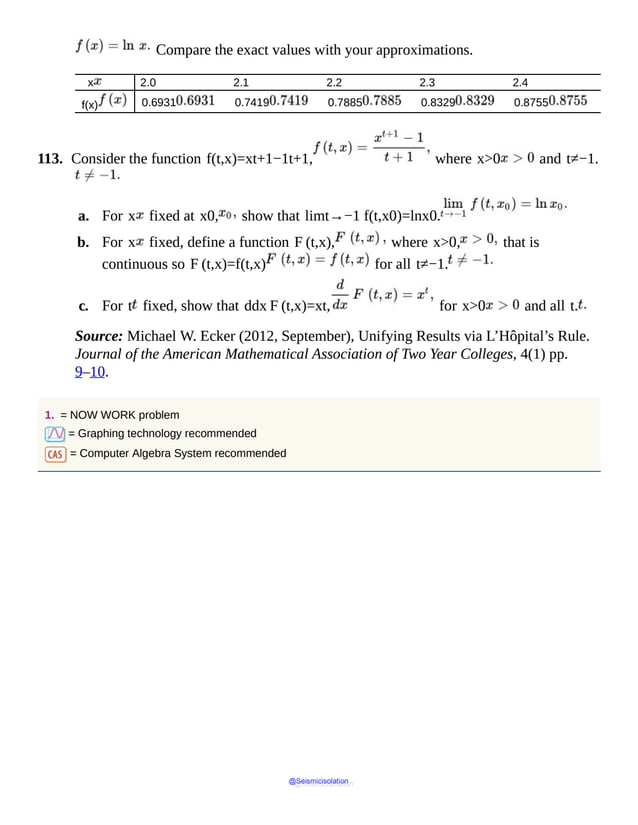
889. is the only one to check—do you see why?]
limx→0− 6x2−6x3=∞limx→0+ 6x2−6x3=−∞
The line x=0 is a vertical asymptote. Draw the asymptotes on the graph.
Step 3
f′(x) =ddx6x2−6x3=12x(x3)−(6x2−6)(3x2)x6Use the Quotient Rule. =
−6x4+18x2x6=6x2(3−x2)x6=6(3−x2)x4f′′(x) =ddx6(3−x2)x4=6⋅(−2x)x4−(3−x2)
(4x3)x8Use the Quotient Rule. =6⋅2x5−12x3x8=12(x2−6)x5
Critical numbers occur where f′(x)=0 or where f′(x) does not exist.
Since f′(x)=0 when x=±3, there are two critical numbers, 3 and
−3. (The derivative does not exist at 0, but, since 0 is not in the domain of f,
it is not a critical number.)
Step 4 Use the numbers −3, 0, and 3 to form four intervals on the x -axis: (−∞,
−3), (−3,0), (0,3) and (3,∞). Then
determine the sign of F′(x) on each interval.
Interval Sign of f′ Conclusion
(−∞,−3) negative f is decreasing on (−∞,−3)
(−3,0) positive f is increasing on (−3,0)
(0,3) positive f is increasing on (0,3)
(3,∞) negative f is decreasing on (3,∞)
Step 5 Use the First Derivative Test. From the table in Step 4, we conclude
f(−3)=−43≈−2.309 is a local minimum value
@Seismicisolation
@Seismicisolation

890. f(3)=43≈ 2.309 is a local maximum value
Plot the local extreme points.
Step 6 Use the Test for Concavity. f′′(x)=12(x2−6)x5=0 when x=
±6. Now use the numbers −6, 0, and 6 to form four intervals on
the x -axis: (−∞,−6),(−6,0),(0,6) and (6,∞).
Then determine the sign of f′′(x) on each interval.
Interval Sign of f′′ Conclusion
(−∞,−6) negative
f is concave down on (−∞,
−6)
(−6,0) positive f is concave up on (−6,0)
(0,6) negative f is concave down on (0,6)
(6,∞) positive f is concave up on (6,∞)
The concavity of the function f changes at −6, 0, and 6. So, the
points −6,−566 and 6,566 are inflection points. Since 0
is not in the domain of f, there is no inflection point at 0. Plot the inflection points.
Step 7 Now use the information about where the function increases/decreases and the
concavity to complete the graph. See Figure 50. Notice the apparent symmetry of the
graph with respect to the origin. We can verify this symmetry by showing f(−x)=−f(x)
and concluding that f is an odd function.
@Seismicisolation
@Seismicisolation

891. Figure 50 f(x)=6x2−6x3 ▪
NOW WORK Problem 11.
Some functions have a graph with an oblique asymptote. That is, the graph of the
function approaches a line y=mx+b, m≠0, as x becomes unbounded in
either the positive or negative direction.
In general, for a function y=f(x), the line y=mx+b, m≠0, is
an oblique asymptote of the graph of f, if
limx→−∞ [f(x)−(mx+b)]=0orlimx→∞ [f(x)−(mx+b)]=0
In Chapter 1, we saw that rational functions can have vertical or horizontal asymptotes.
Rational functions can also have oblique asymptotes, but cannot have both a horizontal
asymptote and an oblique asymptote.
Rational functions for which the degree of the numerator is 1 more than the degree of the
denominator have an oblique asymptote.
Rational functions for which the degree of the numerator is less than or equal to the
@Seismicisolation
@Seismicisolation

892. degree of the denominator have a horizontal asymptote.
EXAMPLE 3 Using Calculus to Graph a Rational Function
Graph f(x)=x2−2x+6x−3.
Solution
Step 1 f is a rational function; the domain of f is {x|x≠3}. There are no x -
intercepts, since x2−2x+6=0 has no real solutions. (Its discriminant is
negative.) The y -intercept is f(0)=−2. Plot the intercept (0,−2).
Step 2 Identify any vertical asymptotes by checking for infinite limits (3 is the only number
to check). Since limx→3− x2−2x+6x−3=−∞ and
limx→3+ x2−2x+6x−3=∞, the line x=3 is a vertical
asymptote.
The degree of the numerator of f is 1 more than the degree of the denominator, so
f will have an oblique asymptote. We divide x2−2x+6 by x−3 to
find the line y=mx+b.
f(x)=x2−2x+6x−3=x+1+ 9x−3
Since limx→∞ [f(x)−(x+1)]=limx→∞ 9x−3=0,
then y=x+1 is an oblique asymptote
of the graph of f. Draw the asymptotes on the graph.
Step 3
f′(x) =ddxx2−2x+6x−3=(2x−2)(x−3)−(x2−2x+6)(1)(x−3)2 =x2−6x(x−3)2=x(x−6)(x−3)2f′
′(x) =ddxx2−6x(x−3)2=(2x−6)(x−3)2−(x2−6x)[2(x−3)](x−3)4 =(x
−3) (2x2−12x+18)−(2x2−12x)(x−3)4=18(x−3)3
@Seismicisolation
@Seismicisolation

893. f′(x)=0 at x=0 and at x=6. So, 0 and 6 are critical
numbers. The tangent lines are horizontal at 0 and at 6. Since 3 is not in the
domain of f, 3 is not a critical number.
Step 4 Use the numbers 0, 3, and 6 to form four intervals on the x -axis: (−∞,0),
(0, 3), (3, 6) and (6,∞). Then determine the sign of F′(x) on
each interval.
Interval Sign of f′(x) Conclusion
(−∞,0) positive f is increasing on (−∞,0)
(0,3) negative f is decreasing on (0,3)
3,6 negative f is decreasing on 3,6
6,∞ positive f is increasing on 6,∞
Step 5 Using the First Derivative Test, we find that f(0)=−2 is a local maximum
value and f(6)=10 is a local minimum value. Plot the points 0,−2
and 6,10.
Step 6 f′′(x)=18(x−3)3. If x<3, f′′(x)<0, and if x>3,
f′′(x)>0. From the Test for Concavity, we conclude f is concave
down on the interval −∞,3 and f is concave up on the interval (3,∞).
The concavity changes at 3, but 3 is not in the domain of f. So, the graph of f
has no inflection point.
@Seismicisolation
@Seismicisolation

894. Step 7 Use the information to complete the graph of the function. See Figure 51.
▪
Figure 51 f(x)=x2−2x+6x−3
NOW WORK Problem 13.
EXAMPLE 4 Using Calculus to Graph a Function
Graph f(x)=xx2+4.
NEED TO REVIEW? Properties of Limits at Infinity are discussed in Section 1.5, pp. 129–131.
Solution
Step 1 The domain of f is all real numbers. The only intercept is (0,0). Plot the point
(0,0).
Step 2 Check for horizontal asymptotes. Since
limx→∞ f(x)=limx→∞ xx2+4=limx→∞ x2x2+4=1
@Seismicisolation
@Seismicisolation

895. the line y=1 is a horizontal asymptote as x→∞. Since limx→−∞ f(x)=
−1, the line y=−1 is also a horizontal asymptote as x→−∞.
Draw the horizontal asymptotes on the graph.
Since f is defined for all real numbers, there are no vertical asymptotes.
Step 3
f′(x) =ddxxx2+4=1⋅x2+4−x12 (x2+4)−1⁄2⋅2xx2+4 =x2+4
− x2x2+4x2+4=x2+4−x2(x2+4)x2+4=4(x2+4)3⁄2f′′(x)
=ddx4(x2+4)3⁄2=4−32 (x2+4)−5⁄2⋅2x=−12x(x2+4)5⁄2
Since f′(x) is never 0 and f′ exists for all real numbers, there are no critical
numbers.
Step 4 Since f′(x)>0 for all x, f is increasing on (−∞,∞).
Step 5 Because there are no critical numbers, there are no local extreme values.
Step 6 Test for concavity. Since f′′(x)>0 on the interval (−∞,0), f is
concave up on (−∞,0); and since f′′(x)<0 on the interval (0,∞),
f is concave down on (0,∞). The concavity changes at 0, and 0
is in the domain of f, so the point (0,0) is an inflection point of f. Plot the
inflection point.
Step 7 Figure 52 shows the graph of f. ▪
@Seismicisolation
@Seismicisolation

896. Figure 52 f(x)= xx2+4
Notice the apparent symmetry of the graph with respect to the origin. We can verify this
by showing f(−x)=−f(x), that is, by showing f is an odd function.
NOW WORK Problem 25.
EXAMPLE 5 Using Calculus to Graph a Function
Graph f(x)=4x1⁄3−x4⁄3.
Solution
Step 1 The domain of f is all real numbers. Since f(0)=0, the y -intercept is 0.
Now f(x)=0 when 4x1⁄3−x4⁄3=x1⁄34−x=0 or
when x=0 or x=4. So, the x -intercepts are 0 and 4. Plot the
intercepts (0,0) and 4,0.
Step 2 Since limx→± ∞ f(x)=limx→± ∞ [x1⁄3(4−x)]=−∞,
there is no horizontal asymptote. Since
the domain of f is all real numbers, there is no vertical asymptote.
Step 3
f′(x)=ddx (4x1⁄3−x4⁄3)=43 x−2⁄3−43 x1⁄3=43 1x2⁄3−x1⁄3=43⋅1−xx2⁄3f′′(x)=ddx 43 x
−2⁄3−43 x1⁄3=−89 x−5⁄3−49 x−2⁄3=−49 2x5⁄3+1x2⁄3=−49⋅2+xx5⁄3
@Seismicisolation
@Seismicisolation

897. Since f′(x)=43⋅1−xx2⁄3=0 when x=1 and f′(x)
does not exist at x=0, the critical numbers are 0 and 1. At the point (1,3),
the tangent line to the graph is horizontal; at the point (0,0), the tangent
line is vertical. Plot these points.
Step 4 Use the critical numbers 0 and 1 to form three intervals on the x -axis: (−∞,0),
(0, 1) and (1, ∞ ). Then determine the sign of F′(x) on each
interval.
Interval Sign of f′ Conclusion
(−∞,0) positive f is increasing on (−∞,0)
(0,1) positive f is increasing on (0,1)
(1,∞) negative f is decreasing on (1,∞)
Step 5 By the First Derivative Test, f(1)=3 is a local maximum value and f(0)=0
is not a local extreme value.
Step 6 Now test for concavity by using the numbers −2 and 0 to form three intervals on
the x -axis: (−∞,−2), (−2,0) and (0, ∞ ). Then determine the
sign of f′′(x) on each interval.
Interval Sign of f″ Conclusion
(−∞,−2) negative
f is concave down on the interval (−∞,
−2)
(−2,0) positive f is concave up on the interval (−2,0)
(0,∞) negative
f is concave down on the interval
(0,∞)
The concavity changes at −2 and at 0. Since
@Seismicisolation
@Seismicisolation

898. f(−2)=4(−2)1⁄3−(−2)4⁄3=4−23−163≈−7.560,
the inflection points are (−2,−7.560) and (0,0). Plot the inflection
points.
Step 7 The graph of f is given in Figure 53.
▪
Figure 53 f(x)=4x1⁄3−x4⁄3
NOW WORK Problem 19.
EXAMPLE 6 Using Calculus to Graph a Trigonometric Function
Graph f(x)=sin x−cos2 x, 0≤x≤2π.
Solution
Step 1 The domain of f is {x|0≤x≤2π}. Since f(0)=sin 0−cos2 0=−1,
the y -intercept is −1. The x -intercepts satisfy the
equation
sin x−cos2 x=sin x−(1−sin2 x)=sin2 x+sin x−1=0
This trigonometric equation is quadratic in form, so we use the quadratic formula.
@Seismicisolation
@Seismicisolation

899. sin x=−1±1−4(1)(−1)2=−1±52
Since −1−52<−1 and −1≤sin x≤1, the x -intercepts
occur at x=sin−1−1+52≈0.666 and at x=π−sin
−1−1+52≈2.475. Plot the intercepts.
NEED TO REVIEW? Trigonometric equations are discussed in Section P. 7, pp. 65–66.
Step 2 The function f has no asymptotes.
Step 3
F′(x) =ddx (sin x−cos2x)=cos x+2 cos x sin x=cos x(1+2 sin x)f
″(x)=ddx[cos x(1+2 sin x)]=2 cos2x−sin x(1+2 sin x)=2 cos2x−sin x−2 sin2x=−4 sin2x
−sin x+2
The critical numbers occur where f′(x)=0. That is, where
cos x=0or1+2 sin x=0
In the interval [0,2π]: cos x=0 if x=π2 or if x=3π2;
and 1+2 sin x=0 when sin x=−12, that is, when
x=7π6 or x=11π6. So, the critical numbers are π2, 7π6, 3π2,
and 11π6. At each of these numbers, the tangent lines are horizontal.
Step 4 Use the numbers 0, π2, 7π6, 3π2, 11π6, and 2π to form five
@Seismicisolation
@Seismicisolation

900. intervals: 0,π2, π2,7π6, 7π6,3π2, 3π2,11π6,
and 11π6,2π. Then determine the sign of f′(x) on each
interval.
Interval Sign of f′ Conclusion
0,π2
positive
f is increasing on 0,π2
π2,7π6
negative
f is decreasing on π2,7π6
7π6,3π2
positive
f is increasing on 7π6,3π2
3π2,11π6
negative
f is decreasing on 3π2,11π6
11π6,2π
positive
f is increasing on 11π6,2π
Step 5 By the First Derivative Test, f π2=1 and f 3π2=−1 are local
maximum values, and f 7π6=−54 and f 11π6=−54
are local minimum values. Plot these points.
Step 6 Use the Test for Concavity. To solve f′′(x)>0 and f′′(x)<0, we
first solve the equation f′′(x)=−4 sin2 x−sin x+2=0,
or equivalently,
4 sin2 x+sin x−2=00≤x≤2πsin x= −1±1+328sin x≈0.593orsin x≈
−0.843x≈0.63x≈2.51x≈4.14x≈5.28
Use these numbers to form five subintervals of [0,2π] and determine the sign
of f′′(x) on each interval.
@Seismicisolation
@Seismicisolation

901. Interval Sign of f′′ Conclusion
(0,0.63) positive
f is concave up on the interval
(0,0.63)
(0.63,2.51) negative
f is concave down on the interval
(0.63,2.51)
(2.51,4.14) positive
f is concave up on the interval
(2.51,4.14)
(4.14,5.28) negative
f is concave down on the interval
(4.14,5.28)
(5.28,2π) positive
f is concave up on the interval
(5.28,2π)
The inflection points are (0.63,−0.06), (2.51,−0.06),
(4.14,−1.13), and (5.28,−1.13). Plot the inflection points.
Step 7 The graph of f is given in Figure 54.
▪
Figure 54 f(x)=sin x−cos2x, 0≤x≤2π
NOTE The function f in Example 6 is periodic with period 2π. To graph this function over its unrestricted
domain, the set of real numbers, repeat the graph in Figure 54 over intervals of length 2π.
@Seismicisolation
@Seismicisolation

902. NOW WORK Problem 33.
EXAMPLE 7 Using Calculus to Graph a Function
Graph f(x)=ex(x2−3).
Solution
Step 1 The domain of f is all real numbers. Since f(0)=−3, the y -intercept is
−3. The x -intercepts occur where
f(x)=ex(x2−3)=0x=3orx=−3
Plot the intercepts.
Step 2 Since the domain of f is all real numbers, there are no vertical asymptotes. To
determine if there are any horizontal asymptotes, we find the limits at infinity. First
we find
limx→− ∞ f(x)=limx→− ∞ [ex(x2−3)]
Since ex(x2−3) is an indeterminate form at −∞ of the type 0⋅∞,
we write ex(x2−3)=x2−3e−x and use L’Hôpital’s Rule.
▪
The line y=0 is a horizontal asymptote as x→−∞.
Since limx→∞ [ex(x2−3)]=∞, there is no horizontal
asymptote as x→∞. Draw the asymptote on the graph.
Step 3
f′(x) =ddx[ex(x2−3)]=ex(2x)+ex(x2−3)=ex(x2+2x−3)= ex(x+3)(x−1)f′′(x)= ddx[ex(x2+2x
−3)]=ex(2x+2)+ex(x2+2x−3) =ex(x2+4x−1)
@Seismicisolation
@Seismicisolation

903. Solving f′(x)=0, we find that the critical numbers are −3 and 1.
Step 4 Use the critical numbers −3 and 1 to form three intervals on the x -axis: (−∞,
−3), (−3,1) and (1,∞). Then determine the sign of F′(x)
on each interval.
Interval Sign of f′ Conclusion
(−∞,−3) positive
f is increasing on the interval (−∞,
−3)
(−3,1) negative f is decreasing on the interval (−3,1)
(1,∞) positive f is increasing on the interval (1,∞)
Step 5 Use the First Derivative Test to identify the local extrema. From the table in Step 4,
there is a local maximum at −3 and a local minimum at 1. Then f(−3)=6e
−3≈0.30 is a local maximum value and f(1)=−2e≈−5.44
is a local minimum value. Plot the local extrema.
Step 6 To determine the concavity of f, first we solve f′′(x)=0. We find x=
−2±5. Now use the numbers −2−5≈−4.24 and
−2+5≈0.24 to form three intervals on the x -axis: (−∞,−2−5),
(−2−5,−2+5) and (−2+5,∞).
Then apply the Test for Concavity.
Interval Sign of f″ Conclusion
(−∞,−2−5) positive f is concave up on the interval
(−∞,−2−5)
(−2−5,−2+5) negative f is concave down on the interval
(−2−5,−2+5)
@Seismicisolation
@Seismicisolation

904. (−2+5,∞) positive f is concave up on the interval
(−2+5,∞)
The inflection points are (−4.24,0.22) and (0.24,−3.73).
Plot the inflection points.
Step 7 The graph of f is given in Figure 55.
▪
Figure 55 f(x)=ex(x2−3)
NOW WORK Problem 39.
4.6 Assess Your Understanding
Skill Building
In Problems 1–42, use calculus to graph each function. Follow the steps for graphing a
function on page 321.
1. f(x)=x4−6x2+10
2. f(x)=x4−4x
@Seismicisolation
@Seismicisolation

905. 3. f(x)=x5−10x2
4. f(x)=x5−3x3+4
5. f(x)=3x5+5x4
6. y=60x5+20x3
7. f(x)=2x2−4
8. f(x)=1x2−1
9. f(x)=2x−1x+1
10. f(x)=x−2x
11. f(x)=xx2+1
12. f(x)=2xx2−4
13. f(x)=x2+12x
14. f(x)=x2−12x
15. f(x)=x2−1x2+2x−3
16. f(x)=x2−x−12x2−9
17. f(x)=x(x3+1)(x2−4)(x+1)
18. f(x)=x(x3−1)(x+1)2(x−1)
19. f(x)=1+1x+1x2
@Seismicisolation
@Seismicisolation

906. 20. f(x)=2x+1x2
21. f(x)=3−x
22. f(x)=xx+2
23. f(x)=x+x
24. f(x)=x−x+1
25. f(x)=x2x+1
26. f(x)=xx2+2
27. f(x)=1(x+1)(x−2)
28. f(x)=1(x−1)(x+3)
29. f(x)=x2⁄3+3x1⁄3+2
30. f(x)=x5⁄3−5x2⁄3
31. f(x)=sin x−cos x
32. f(x)=sin x+tan x
33. f(x)=sin2 x−cos x
34. f(x)=cos2 x+sin x
35. y=ln x−x
36. y=x ln x
37. f(x)=ln(4−x2)
38. y=ln(x2+2)
39. f(x)=3e3x(5−x)
40. f(x)=3e−3x(x−4)
41. f(x)=e−x2
@Seismicisolation
@Seismicisolation

907. 42. f(x)=e1⁄x
Applications and Extensions
In Problems 43–52, for each function:
a. Graph the function.
b. Identify any asymptotes.
c. Use the graph to identify intervals on which the function increases or decreases and the
intervals where the function is concave up or down.
d. Approximate the local extreme values using the graph.
e. Compare the approximate local maxima and local minima to the exact local extrema
found by using calculus.
f. Approximate any inflection points using the graph.
43. f(x)=x2⁄3x−1
44. f(x)=5−xx2+3x+4
45. f(x)=x+sin (2x)
46. f(x)=x−cos x
47. f(x)=ln(xx−1)
48. f(x)=ln(tan2 x)
49. f(x)=sin x3
50. f(x)=e−x cos x
51. y2=x2(6−x), y≥0
52. y2=x2(4−x2), y≥0
In Problems 53–56, graph a function f that is continuous on the interval [1,6] and
satisfies the given conditions.
53. f′(2) does not existf′(3)=−1f′′(3)=0f′(5)=0f′′(x)<0,2<x<3f′′(x)>0,x>3
@Seismicisolation
@Seismicisolation

908. 54. f′(2)=0f′′(2)=0f′(3) does not existf′(5)=0f′′(x)>0,2<x<3f′′(x)>0,x>3
55. f′(2)=0limx→3− f′(x)=∞limx→3+ f′(x)=∞f′(5)=0f′′(x)>0,x<3f′′(x)<0,x>3
56. f′(2)=0limx→3− f′(x)=−∞limx→3+ f′(x)=−∞f′(5)=0f′′(x)<0,x<3f′′(x)>0,x>3
57. Graph a function f defined and continuous for −1≤x≤2 that satisfies the
following conditions:
f(−1)=1f(1)=2f(2)=3f(0)=0f 12=3limx→−1+ f′(x)=−∞limx→1− f′(x)=−1limx→1+ f
′(x)=∞f has a local minimum at 0f has a local minimum at 12
@Seismicisolation
@Seismicisolation

909. 58. Graph of a Function Which of the following is true about the graph of y=ln|x2−1|
in the interval (−1,1)?
a. The graph is increasing.
b. The graph has a local minimum at (0,0).
c. The graph has a range of all real numbers.
d. The graph is concave down.
e. The graph has an asymptote x=0.
59. Properties of a Function Suppose f(x)=1x+ln x is defined only on the
closed interval 1e≤x≤e.
a. Determine the numbers x at which f has its absolute maximum and absolute
minimum.
b. For what numbers x is the graph concave up?
c. Graph f.
60. Probability The function f(x)=12π e−x2⁄2, encountered in
probability theory, is called the standard normal density function. Determine where
this function is increasing and decreasing, find all local maxima and local minima, find
all inflection points, and determine the intervals where f is concave up and concave
down. Then graph the function.
In Problems 61–64, graph each function. Use L’Hôpital’s Rule to find any asymptotes.
61. f(x)=sin (3x)x4−x2
62. f(x)=xx
63. f(x)=x1⁄x
@Seismicisolation
@Seismicisolation

910. 64. y=1x tan x−π2<x<π2
1. = NOW WORK problem
= Graphing technology recommended
= Computer Algebra System recommended
@Seismicisolation
@Seismicisolation

911. 4.7 Optimization
OBJECTIVE When you finish this section, you should be able to:
1 Solve optimization problems
Investigating maximum and/or minimum values of a function has been a recurring theme
throughout most of this chapter. We continue this theme, using calculus to solve optimization
problems.
Optimization is a process of determining the best solution to a problem. Often the best
solution is one that maximizes or minimizes some quantity. For example, a business owner’s
goal usually involves minimizing cost while maximizing profit, or an engineer’s goal may be
to minimize the load on a beam. In this section, we model optimization problems using a
function.
1 Solve Optimization Problems
Even though each individual problem has unique features, it is possible to outline a general
method for obtaining an optimal solution.
Steps for Solving Optimization Problems
Step 1 Read the problem until you understand it and can identify the quantity for which a
maximum or minimum value is to be found. Assign a symbol to represent it.
Step 2 Assign symbols to represent the other variables in the problem. If possible, draw a
picture and label it. Determine relationships among the variables.
Step 3 Express the quantity to be maximized or minimized as a function of one of the
variables, and determine a meaningful domain for the function.
Step 4 Find the absolute maximum value or absolute minimum value of the function.
NOTE It is good practice to have in mind meaningful estimates of the answer.
EXAMPLE 1 Maximizing an Area
A farmer with 4000 m of fencing wants to enclose a rectangular plot that borders a
straight river, as shown in Figure 56. If the farmer does not fence the side along the river,
what is the largest rectangular area that can be enclosed?
@Seismicisolation
@Seismicisolation

912. Figure 56 Area A=xy
Solution
Step 1 The quantity to be maximized is the area; we denote it by A.
Step 2 We denote the dimensions of the rectangle by x and y (both in meters), with the
length of the side y parallel to the river. The area is A=xy. Because there
are 4000 m of fence available, the variables x and y are related by the
equation
x+y+x=4000y=4000−2x
Step 3 Now express the area A as a function of x.
A=A(x)=x(4000−2x)=4000x−2x2A=xy,y=4000−2x
The domain of A is the closed interval [0,2000].
Step 4 To find the number x that maximizes A(x), differentiate A with respect to
x and find the critical numbers:
A′(x)=4000−4x=0
NOTE Since A=A(x) is continuous on the closed interval [0, 2000], it will have an absolute
maximum.
The only critical number is x=1000. The maximum value of A occurs
either at the critical number or at an endpoint of the interval [0,2000].
@Seismicisolation
@Seismicisolation

913. A(1000)=2,000,000A(0)=0A(2000)=0
The maximum value is A(1000)=2,000,000 m2, which
results from fencing a rectangular plot that measures 2000 m along the side
parallel to the river and 1000 m along each of the other two sides.
▪
We could have reached the same conclusion by noting that A′′(x)=−4<0
for all x, so A is always concave down, and the local maximum at x=1000
must be the absolute maximum of the function.
NOW WORK Problem 3.
EXAMPLE 2 Maximizing a Volume
From each corner of a square piece of sheet metal 18 cm on a side, remove a small
square and turn up the edges to form an open box. What are the dimensions of the box with
the largest volume?
Solution
Step 1 The quantity to be maximized is the volume of the box; denote it by V. Denote the
length of each side of the small squares by x and the length of each side after the
small squares are removed by y, as shown in Figure 57. Both x and y are in
centimeters.
@Seismicisolation
@Seismicisolation

914. Figure 57 y=18−2x
Step 2 Then y=(18−2x) cm. The height of the box is x cm, and the
area of the base of the box is y2 cm2. So, the volume of the box is
V=xy2 cm3.
Step 3 To express V as a function of one variable, substitute y=18−2x into the
formula for V. Then the function to be maximized is
V=V(x)=x(18−2x)2
Since both x≥0 and 18−2x≥0, we find x≤9, meaning the
domain of V is the closed interval [0,9]. (All other numbers make no physical
sense—do you see why?)
Step 4 To find the value of x that maximizes V, differentiate V and find the critical
numbers.
Now solve V′(x)=0 for x. The solutions are
x=9orx=3
The only critical number in the open interval (0,9) is 3. Evaluate V at 3 and
@Seismicisolation
@Seismicisolation

915. at the endpoints 0 and 9.
V(0)=0V(3)=3(18−6)2=432V(9)=0
The maximum volume is 432 cm3. The box with the maximum volume
has a height of 3 cm. Since y=18−2(3)=12 cm, the base of
the box is square and measures 12 cm by 12 cm. ▪
NOW WORK Problems 7 and 9.
EXAMPLE 3 Maximizing an Area
A manufacturer makes a flexible square play yard (Figure 58a), with hinges at the four
corners. It can be opened at one corner and attached at right angles to a wall or the side of a
house, as shown in Figure 58(b). If each side is 3 m in length, the open configuration
doubles the available area from 9 m2 to 18 m2. Is there a configuration that will
more than double the play area?
Figure 58
Solution
Step 1 We want to maximize the play area A.
Step 2 Since the play yard must be attached at right angles to the wall, the possible
configurations depend on the amount of wall used as a fifth side, as shown in Figure
59. Use x to represent half the length (in meters) of the wall used as the fifth side.
@Seismicisolation
@Seismicisolation

916. Figure 59
Step 3 Partition the play area into two sections: a rectangle with area 3⋅2x=6x and
a triangle with base 2x and altitude 32−x2=9−x2. The play
area A is the sum of the areas of the two sections. The area to be maximized is
A=A(x)=6x+12 (2x)9−x2=6x+x9−x2
The domain of A is the closed interval [0,3].
Step 4 To find the maximum area of the play yard, find the critical numbers of A.
A′(x) = 6+x[12 (−2x)(9−x2)−1⁄2]+9−x2 Use the Sum Rule and Product Rule. =
6−x29−x2+9−x2=69−x2−2x2+99−x2
@Seismicisolation
@Seismicisolation

917. Critical numbers occur when A′(x)=0 or where A′(x) does not exist. A′
does not exist at −3 and 3, and A′(x)=0 at
matrix
Element
1
1
six
Square
root
of
nine
minus
x
square
minus
two
x
square
plus
nine
Element
2
1
equals
Element
3
The only critical number in the open interval (0,3) is 24344≈2.792.
Now evaluate A(x) at the endpoints 0 and 3 and at the critical number
x≈2.792.
A(0)=0A(3)=18A(2.792)≈19.817
Using a wall of length 2x≈2(2.792)=5.584 m maximizes the
area; the configuration shown in Figure 60 increases the play area by approximately
10% (from 18 to 19.817 m2 ).
▪
@Seismicisolation
@Seismicisolation

918. Figure 60 Area≈19.817 m 2
EXAMPLE 4 Minimizing Cost
A manufacturer needs to produce a cylindrical container with a capacity of 1000 cm3.
The top and bottom of the container are made of material that costs $0.05 per
square centimeter, while the side of the container is made of material costing $0.03 per
square centimeter. Find the dimensions that will minimize the company’s cost of producing
the container.
Solution Figure 61 shows a cylindrical container and the area of its top, bottom, and lateral
surface. As shown in the figure, let h denote the height of the container and R denote the
radius. The total area of the bottom and top is 2πR2 cm2. The area of the lateral
surface of the can is 2π Rh cm2.
@Seismicisolation
@Seismicisolation

919. Figure 61
The variables h and R are related. Since the capacity (volume) V of the cylinder is
1000 cm3,
V=πR2h=1000h=1000πR2
NEED TO REVIEW? Geometry formulas are discussed in Appendix A.2, p. A-15.
The cost C, in dollars, of manufacturing the container is
matrix
Element
1
1
Element
2
1
cap
c
equals
left
parenthesis
0.05
By substituting for h, C can be expressed as a function of R.
C=C(R)=0.1πR2+(0.06π R)1000πR2=0.1πR2+60R
This is the function to be minimized. The domain of C is R|R>0.
To find the minimum cost, differentiate C with respect to R.
C′(R)=0.2π R− 60R2=0.2πR3−60R2
Solve C′(R)=0 to find the critical numbers.
@Seismicisolation
@Seismicisolation

920. 0.2πR3−60=0R3=300πR=300π3≈4.571 cm
Now find C″(R) and use the Second Derivative Test.
C″(R)=ddR 0.2πR− 60R2=0.2π+120R3C″300π3=0.2π+120π300=0.6π>0
NOTE If the costs of the materials for the top, bottom, and lateral surfaces of a cylindrical container are all
equal, then the minimum total cost occurs when the surface area is minimum. It can be shown (see Problem
39) that for any fixed volume, the minimum surface area of a cylindrical container is obtained when the height
equals twice the radius.
C has a local minimum at 300π3. Since C″(R)>0 for all R in the
domain, the graph of C is always concave up, and the local minimum value is the absolute
minimum value. The radius of the container that minimizes the cost is R≈4.571 cm.
The height of the container that minimizes the cost of the material is
h=1000πR2≈ 100020.892π≈15.236 cm
The minimum cost of the container is
C 300π3=0.1π300π3 2+60300π3≈$19.69 ▪
NOW WORK Problem 11.
EXAMPLE 5 Maximizing Area
A rectangle is inscribed in a semicircle of radius 2. Find the dimensions of the rectangle
that has the maximum area.
@Seismicisolation
@Seismicisolation

921. Solution We present two methods of solution: The first uses analytic geometry, the second
uses trigonometry. To begin, place the semicircle with its diameter along the x -axis and
center at the origin. Then inscribe a rectangle in the semicircle, as shown in Figure 62. The
length of the inscribed rectangle is 2x and its height is y.
Figure 62
Analytic Geometry Method The area A of the inscribed rectangle is A=2xy and
the equation of the semicircle is x2+y2=4, y≥0. We solve for y in
x2+y2=4 and obtain y=4−x2. Now substitute this expression for y
in the area formula for the rectangle to express A as a function of x alone.
Then using the Product Rule,
A
′(x)=2[x⋅12{4−x2)−1⁄2(−2x)+4−x2]=2[−x24−x2+4−x2]=2[−x2+4−x24−x2]=2[−2(x2−2)4−x2
−4(x2−2)4−x2
The only critical number in the open interval (0,2) is 2, where A′(2)=0.
@Seismicisolation
@Seismicisolation

922. [The numbers −2 and −2 are not in the domain of A, and 2 is not
in the open interval (0,2). ] The values of A at the endpoints 0 and 2 and at the
critical number 2 are
A(0)=0A(2)=4A(2)=0
The maximum area of the inscribed rectangle is 4, and it corresponds to the rectangle
whose length is 2x=22 and whose height is y=2.
Trigonometry Method Using Figure 62, draw the radius r=2 from O to the vertex of
the rectangle and place the angle θ in the standard position, as shown in Figure 63. Then
x=2 cos θ and y=2 sin θ, 0≤θ≤π2. The area A of the
rectangle is
Figure 63
Since the area A is a differentiable function of θ, we obtain the critical numbers by
finding A′(θ) and solving the equation A′(θ)=0.
A′(θ)=8 cos (2θ)=0A(θ)=4sin(2θ) cos (2θ)=02θ=cos−1 0=π2θ=π4
@Seismicisolation
@Seismicisolation

923. Now find A′′(θ) and use the Second Derivative Test.
A″(θ)=−16 sin (2θ)A″π4=−16 sin 2⋅π4=−16 sin π2=−16<0
So at θ=π4, the area A is maximized and the maximum area of the inscribed
rectangle is
A π4=4 sin 2⋅π4=4 square units
The rectangle with the maximum area has
length 2x=4 cos π4=22 and height y=2 sin π4=2 ▪
NOW WORK Problem 41.
EXAMPLE 6 Snell’s Law of Refraction
Light travels at different speeds in different media (air, water, glass, etc.). Suppose that light
travels from a point A in one medium, where its speed is c1, to a point B in another
medium, where its speed is c2. See Figure 64. We use Fermat’s principle that light always
travels along the path that requires the least time to prove Snell’s Law of Refraction.
sin θ1c1=sin θ2c2
@Seismicisolation
@Seismicisolation

924. Figure 64
ORIGINS In 1621 Willebrord Snell (c. 1580–1626) discovered the law of refraction, one of the basic principles
of geometric optics. Pierre de Fermat (1601–1665) was able to prove the law mathematically using the principle
that light follows the path that takes the least time.
Solution Position the coordinate system, as illustrated in Figure 65. The light passes from
one medium to the other at the point P. Since the shortest distance between two points is a
line, the path taken by the light is made up of two line segments—from A=(0,a) to
P=(x,0) and from P=(x,0) to B=(k,−b), where a,b, and
k are positive constants.
@Seismicisolation
@Seismicisolation

925. (1)
Figure 65
The
path
taken
by
the
light
is
made
up
of
two
line
segments:
from
A
(0,
a)
to
P
(x,
0)
and
from
P
(x,
Since
Time=DistanceSpeed
the travel time t1 from A=(0,a) to P=(x,0) is
t1=x2+a2c1 c1 is the speed of light in medium 1.
and the travel time t2 from P=(x,0) to B=(k,−b) is
t2=(k−x)2+b2c1 c2 is the speed of light in medium 2.
The total time T=T(x) is given by
T(x)=t1+t2=x2+a2c1+(k−x)2+b2c2
To find the least time, find the critical numbers of T.
@Seismicisolation
@Seismicisolation

926. (2)
T′(x)= xc1x2+a2− k−xc2(k−x)2+b2=0
From Figure 65,
xx2+a2=sin θ1and k−x(k−x)2+b2=sin θ2
Using the result from (2) in equation (1), we have
T′(x)=sin θ1c1−sin θ2c2=0sin θ1c1=sin θ2c2
Now to be sure that the minimum value of T occurs when T′(x)=0, we show
that T″(x)>0. From (1),
T″(x)=ddx xc1x2+a2− ddx k−xc2(k−x)2+b2=a2c1(x2+a2)3⁄2+ b2c2[(k−x)2+b2]3⁄2>0
Since T″(x)>0 for all x, T is concave up for all x, and the minimum value
of T occurs at the critical number. That is, T is a minimum when sin θ1c1=sin θ2c2. ▪
4.7 Assess Your Understanding
Applications and Extensions
1. Maximizing Area The owner of a motel has 3000 m of fencing and wants to enclose a
rectangular plot of land that borders a straight highway. If she does not fence the side
along the highway, what is the largest area that can be enclosed?
2. Maximizing Area If the motel owner in Problem 1 decides to also fence the side along
the highway, except for 5 m to allow for access, what is the largest area that can be
@Seismicisolation
@Seismicisolation

927. enclosed?
3. Maximizing Area Find the dimensions of the rectangle with the largest area that can be
enclosed on all sides by L meters of fencing.
4. Maximizing the Area of a Triangle An isosceles triangle has a perimeter of fixed
length L. What should the dimensions of the triangle be if its area is to be a
maximum? See the figure.
5. Maximizing Area A gardener with 200 m of available fencing wishes to enclose
a rectangular field and then divide it into two plots with a fence parallel to one of the
sides, as shown in the figure. What is the largest area that can be enclosed?
6. Minimizing Fencing A realtor wishes to enclose 600 m2 of land in a rectangular
plot and then divide it into two plots with a fence parallel to one of the sides. What are
the dimensions of the rectangular plot that require the least amount of fencing?
7. Maximizing the Volume of a Box An open box with a square base is to be made from a
square piece of cardboard that measures 12 cm on each side. A square will be cut
out from each corner of the cardboard and the sides will be turned up to form the box.
Find the dimensions that yield the maximum volume.
@Seismicisolation
@Seismicisolation

928. 8. Maximizing the Volume of a Box An open box with a rectangular base is to be made
from a piece of tin measuring 30 cm by 45 cm by cutting out a square from
each corner and turning up the sides. Find the dimensions that yield the maximum
volume.
9. Minimizing the Surface Area of a Box An open box with a square base is to have a
volume of 2000 cm3. What should the dimensions of the box be if the amount
of material used is to be a minimum?
10. Minimizing the Surface Area of a Box If the box in Problem 9 is to be closed on top,
what should the dimensions of the box be if the amount of material used is to be a
minimum?
11. Minimizing the Cost to Make a Can A cylindrical container that has a capacity of
10 m3 is to be produced. The top and bottom of the container are to be made of a
material that costs $20 per square meter, while the side of the container is to be
made of a material costing $15 per square meter. Find the dimensions that will
minimize the cost of the material.
12. Minimizing the Cost of Fencing A builder wishes to fence in 60, 000 m2 of
land in a rectangular shape. For security reasons, the fence along the front part of the
land will cost $20 per meter, while the fence for the other three sides will cost $10
per meter. How much of each type of fence should the builder buy to minimize the
cost of the fence? What is the minimum cost?
13. Maximizing Revenue A car rental agency has 24 cars (each an identical model). The
owner of the agency finds that at a price of $18 per day, all the cars can be rented;
however, for each $1 increase in rental cost, one of the cars is not rented. What
should the agency charge to maximize income?
14. Maximizing Revenue A charter flight club charges its members $200 per year. But
for each new member in excessof 60, the charge for every member is reduced by $2.
What number of members leads to a maximum revenue?
15. Minimizing Distance Find the coordinates of the points on the graph of the parabola
y=x2 that are closest to the point 2,12.
16. Minimizing Distance Find the coordinates of the points on the graph of the parabola
y=2x2 that are closest to the point (1,4).
17. Minimizing Distance Find the coordinates of the points on the graph of the parabola
y=4−x2 that are closest to the point (6,2).
18. Minimizing Distance Find the coordinates of the points on the graph of y=x
@Seismicisolation
@Seismicisolation

929. that are closest to the point (4,0).
19. Minimizing Transportation Cost A truck has a top speed of 75mi⁄h and,
when traveling at a speed of x mi⁄h, consumes gasoline at the rate of
12001600x+x gallons per mile. The truck is to be taken on a 200-mi
trip by a driver who is paid at the rate of $b per hour plus a commission of $c.
Since the time required for the trip at x mi⁄h is 200x, the cost C of the
trip, when gasoline costs $a per gallon, is
C=C(x)=1600x+xa+200xb+c
Find the speed that minimizes the cost C under each of the following conditions:
a. a=$3.50, b=0, c=0
b. a=$3.50, b=$10.00, c=$500
c. a=$4.00, b=$20.00, c=0
20. Optimal Placement of a Cable Box A telephone company is asked to provide cable
service to a customer whose house is located 2 km away from the road along which
the cable lines run. The nearest cable box is located 5 km down the road. As shown
in the figure below, let 5−x denote the distance from the box to the connection so
that x is the distance from this point to the point on the road closest to the house. If the
cost to connect the cable line is $500 per kilometer along the road and $600
per kilometer away from the road, where along the road from the box should the
company connect the cable line so as to minimize construction cost?
@Seismicisolation
@Seismicisolation

930. 21. Minimizing a Path Two houses A and B on the same side of a road are a distance
p apart, with distances q and r, respectively, from the center of the road, as shown
in the figure below. Find the length of the shortest path that goes from A to the road
and then on to the other house B.
a. Use calculus.
b. Use only elementary geometry.
(Hint: Reflect B across the road to a point C that is also a distance r from the
center of the road.)
22. Minimizing Travel Time A small island is 3 km from the nearest point P on the
straight shoreline of a large lake. A town is 12 km down the shore from P. See
the figure. If a person on the island can row a boat 2.5 km⁄h and can walk
4 km⁄h, where should the boat be landed so that the person arrives in town in the
shortest time?
@Seismicisolation
@Seismicisolation

931. 23. Supporting a Wall Find the length of the shortest beam that can be used to brace a wall
if the beam is to pass over a second wall 2 m high and 5 m from the first wall.
See the figure. What is the angle of elevation of the beam?
24. Maximizing the Strength of a Beam The strength of a rectangular beam is proportional
to the product of the width and the cube of its depth. Find the dimensions of the
strongest beam that can be cut from a log whose cross section has the form of a circle of
fixed radius R. See the figure.
@Seismicisolation
@Seismicisolation

932. 25. Maximizing the Strength of a Beam If the strength of a rectangular beam is
proportional to the product of its width and the square of its depth, find the dimensions
of the strongest beam that can be cut from a log whose cross section has the form of the
ellipse 10x2+9y2=90.
(Hint: Choose width =2x and depth =2y. )
26. Maximizing the Strength of a Beam The strength of a beam made from a certain wood
is proportional to the product of its width and the cube of its depth. Find the dimensions
of the rectangular cross section of the beam with maximum strength that can be cut from
a log whose original cross section is in the form of the ellipse b2x2+a2y2=a2b2,
a≥b.
27. Pricing Wine A winemaker in Walla Walla, Washington, is producing the first vintage
for her own label, and she needs to know how much to charge per case of wine. It costs
her $132 per case to make the wine. She understands from industry research and an
assessment of her marketing list that she can sell x=1430−116p cases of
wine, where p is the price of a case in dollars. She can make at most 1100 cases
of wine in her production facility. How many cases of wine should she produce, and
what price p should she charge per case to maximize her profit P? (Hint: Maximize
the profit P=xp−132x, where x equals the number of cases.)
28. Optimal Window Dimensions A Norman window has the shape of a rectangle
surmounted by a semicircle of diameter equal to the width of the rectangle, as shown in
the figure. If the perimeter of the window is 10 m, what dimensions will admit the
most light?
@Seismicisolation
@Seismicisolation

933. 29. Maximizing Volume The sides of a V-shaped trough are 28 cm wide. Find the
angle between the sides of the trough that results in maximum capacity.
30. Maximizing Volume A metal rain gutter is to have 10-cm sides and a 10-cm
horizontal bottom, with the sides making equal angles with the bottom, as shown in the
figure. How wide should the opening across the top be for maximum carrying capacity?
31. Minimizing Construction Cost A proposed tunnel with a fixed cross-sectional area is
to have a horizontal floor, vertical walls of equal height, and a ceiling that is a
semicircular cylinder. If the ceiling costs three times as much per square meter to build
as the vertical walls and the floor, find the most economical ratio of the diameter of the
semicircular cylinder to the height of the vertical walls.
@Seismicisolation
@Seismicisolation

934. 32. Minimizing Construction Cost An observatory is to be constructed in the form of a
right circular cylinder surmounted by a hemispherical dome. If the hemispherical dome
costs three times as much per square meter as the cylindrical wall, what are the most
economical dimensions for a given volume? Neglect the floor.
33. Intensity of Light The intensity of illumination at a point varies inversely as the square
of the distance between the point and the light source. Two lights, one having an
intensity eight times that of the other, are 6 m apart. At what point between the two
lights is the total illumination least?
34. Drug Concentration The concentration of a drug in the bloodstream t hours after
injection into muscle tissue is given by C(t)=2t16+t2. When is the
concentration greatest?
35. Optimal Wire Length A wire is to be cut into two pieces. One piece will be bent into a
square, and the other piece will be bent into a circle. If the total area enclosed by the two
pieces is to be 64 cm2, what is the minimum length of wire that can be used?
What is the maximum length of wire that can be used?
36. Optimal Wire Length A wire is to be cut into two pieces. One piece will be bent into
an equilateral triangle, and the other piece will be bent into a circle. If the total area
enclosed by the two pieces is to be 64 cm2, what is the minimum length of wire
that can be used? What is the maximum length of wire that can be used?
37. Optimal Area A wire 35 cm long is cut into two pieces. One piece is bent into the
shape of a square, and the other piece is bent into the shape of a circle.
a. How should the wire be cut so that the area enclosed is a minimum?
b. How should the wire be cut so that the area enclosed is a maximum?
c. Graph the area enclosed as a function of the length of the piece of wire used to make
@Seismicisolation
@Seismicisolation

935. the square. Show that the graph confirms the results of (a) and (b).
38. Optimal Area A wire 35 cm long is cut into two pieces. One piece is bent into the
shape of an equilateral triangle, and the other piece is bent into the shape of a circle.
a. How should the wire be cut so that the area enclosed is a minimum?
b. How should the wire be cut so that the area enclosed is a maximum?
c. Graph the area enclosed as a function of the length of the piece of wire used to make
the triangle. Show that the graph confirms the results of (a) and (b).
39. Optimal Dimensions for a Can Show that a cylindrical container of fixed volume V
requires the least material (minimum surface area) when its height is twice its radius.
40. Maximizing Area Find the triangle of largest area that has two sides along the positive
coordinate axes if its hypotenuse is tangent to the graph of y=3e−x.
41. Maximizing Area Find the largest area of a rectangle with one vertex on the parabola
y=9−x2, another at the origin, and the remaining two on the positive x -
axis and positive y -axis, respectively. See the figure.
42. Maximizing Volume Find the dimensions of the right circular cone of maximum
volume having a slant height of 4 ft. See the figure.
@Seismicisolation
@Seismicisolation

936. 43. Minimizing Distance Let a and b be two positive real numbers. Find the line
through the point (a,b) and connecting the points (0,y0) and (x0,0) so
that the distance from (x0,0) to (0,y0) is a minimum. (In general, x0 and
y0 will depend on the line.)
44. Maximizing Velocity An object moves on the x -axis in such a way that its velocity at
time t seconds, t≥1, is given by v= ln tt cm⁄s. At what time t does
the object attain its maximum velocity?
45. Physics A heavy object of mass m is to be dragged along a horizontal surface by a
rope making an angle θ to the horizontal. The force F required to move the object is
given by the formula
F=cmgc sin θ + cos θ
where g is the acceleration due to gravity and c is the coefficient of friction of the
surface. Show that the force is least when tan θθ=c.
46. Chemistry A self-catalytic chemical reaction results in the formation of a product that
causes its formation rate to increase. The reaction rate V of many self-catalytic
chemicals is given by
V=kx (a−x)0≤x≤a
where k is a positive constant, a is the initial amount of the chemical, and x is the
variable amount of the chemical. For what value of x is the reaction rate a maximum?
47. Optimal Viewing Angle A picture 4 m in height is hung on a wall with the lower
edge 3 m above the level of an observer’s eye. How far from the wall should the
@Seismicisolation
@Seismicisolation

937. observer stand in order to obtain the most favorable view? (That is, the picture should
subtend the maximum angle.)
48. Maximizing Transmission Speed Traditional telephone cable is made up of a core of
copper wires covered by an insulating material. If x is the ratio of the radius of the
core to the thickness of the insulating material, the speed v of signaling is v=kx2ln 1x,
where k is a constant. Determine the ratio x that results in maximum
speed.
49. Absolute Minimum If a, b, and c are positive constants, show that the minimum
value of f(x)=aecx+be−cx is 2ab.
Challenge Problems
50. Maximizing Length The figure shows two corridors meeting at a right angle. One has
width 1 m, and the other, width 8 m. Find the length of the longest pipe that can
be carried horizontally from one corridor, around the corner, and into the other corridor.
@Seismicisolation
@Seismicisolation

938. 51. Optimal Height of a Lamp In the figure, a circular area of radius 20 ft is
surrounded by a walk. A light is placed above the center of the area. What height most
strongly illuminates the walk? The intensity of illumination is given by I=sin θs,
where s is the distance from the source and θ is the angle at which the
light strikes the surface.
52. Maximizing Area Show that the rectangle of largest area that can be inscribed under the
graph of y=e−x2 has two of its vertices at the point of inflection of y. See the
figure.
@Seismicisolation
@Seismicisolation

939. 53. Minimizing Distance Find the point (x,y) on the graph of f(x)=e−x⁄2
that is closest to the point (1,8).
1. = NOW WORK problem
= Graphing technology recommended
= Computer Algebra System recommended
@Seismicisolation
@Seismicisolation

940. 4.8 Antiderivatives; Differential Equations
OBJECTIVES When you finish this section, you should be able to:
1 Find antiderivatives
2 Solve a differential equation
3 Solve applied problems modeled by differential equations
We have already learned that for each differentiable function f, there is a corresponding
derivative function f′. Now consider this question: For a given function f, is there a
function F whose derivative is f? That is, is it possible to find a function F so that f
′=dFdx=f? If such a function F can be found, it is called an antiderivative of
f.
DEFINITION Antiderivative
A function F is called an antiderivative of the function f if f′(x)=f(x) for
all x in the domain of f.
1 Find Antiderivatives
For example, an antiderivative of the function f(x)=2x is F(x)=x2,
since
f′(x)= ddx x2=2x
Another function F whose derivative is 2x is F(x)=x2+3, since
f′(x)= ddx (x2+3)=2x
This leads us to suspect that the function f(x)=2x has many antiderivatives.
Indeed, any of the functions x2 or x2+12 or x2+2 or x2+5 or x2−1
has the property that its derivative is 2x. Any function F(x)=x2+C,
where C is a constant, is an antiderivative of f(x)=2x.
Are there other antiderivatives of 2x that are not of the form x2+C? A
corollary of the Mean Value Theorem (p. 288) tells us the answer is no.
@Seismicisolation
@Seismicisolation

941. COROLLARY
If f and g are differentiable functions and if f′(x)=g′(x) for all numbers x in an interval
(a,b), then there exists a number C for which f(x)=g(x)+C on (a,b).
This result can be stated in the following way.
THEOREM The General Form of an Antiderivative
If a function F is an antiderivative of a function f defined on an interval I, then any
other antiderivative of f has the form F(x)+C, where C is an (arbitrary)
constant.
All the antiderivatives of f can be obtained from the expression F(x)+C by
letting C range over all real numbers. For example, all the antiderivatives of f(x)=x5
are of the form F(x)=x66+C, where C is a constant. Figure 66
shows the graphs of F(x)=x66+C for some numbers C. The
antiderivatives of a function f are a family of functions, each one a vertical translation of
the others.
Figure 66 F(x)=x66+C
EXAMPLE 1 Finding the Antiderivatives of a Function
Find all the antiderivatives of:
@Seismicisolation
@Seismicisolation

942. a. f(x)=0
b. g(θ)=− sin θ
c. h(x)=x1⁄2
Solution a. Since the derivative of a constant function is 0, all the antiderivatives of f
are of the form F(x)=C, where C is a constant.
b. Since ddθ cos θ=− sin θ, all the antiderivatives of g(θ)=− sin θ
are of the form G(θ)=cos θ+C, where C is a constant.
c. The derivative of 23 x3⁄2 is 23⋅32 x3⁄2−1=x1⁄2. So, all the
antiderivatives of h(x)=x1⁄2 are of the form H(x)=23 x3⁄2+C,
where C is a constant. ▪
In Example 1(c), you may wonder how we knew to choose 23 x3⁄2. For any real
number a, the Power Rule states ddx xa=axa−1. That is, differentiation
reduces the exponent by 1. Antidifferentiation is the inverse process, so it suggests we
increase the exponent by 1. This is how we obtain the factor x3⁄2 of the antiderivative
23 x3⁄2. The factor 23 is needed so that when we differentiate 23 x3⁄2, the
result is 23⋅32 x3⁄2−1=x1⁄2.
NOW WORK Problem 11.
Let f(x)=xa, where a is a real number and a≠−1. (The case for
which a=− 1 requires special attention.) Then the function F(x) defined by
F(x)=xa+1a+1a≠−1
is an antiderivative of f(x)=xa. That is, all the antiderivatives of f(x)=xa,
a≠−1, are of the form xa+1a+1+C, where C is a
constant.
Now consider the case when a=− 1. Then f(x)=x−1=1x. We
@Seismicisolation
@Seismicisolation

943. know that ddx ln|x|=1x=x−1, for x≠0. So, all the antiderivatives
of f(x)=x−1 are of the form ln|x|+C, provided x≠0.
CAUTION Be sure to include the absolute value bars when finding the antiderivative of 1x.
Table 6 includes these results along with the antiderivatives of some other common
functions. Each listing is based on a derivative formula.
TABLE 6
Function f Antiderivatives F of f Function f
f(x)=0 F(x)=C f(x)=sec x tan
f(x)=1 F(x)=x+C f(x)=cscxcot x
f(x)=xa, a≠
−1 F(x)=xa+1a+1+C
f(x)=csc 2x
f(x)=x−1=1x F(x)=ln|x|+C f(x)=11−x2,
f(x)=ex F(x)=ex+C f(x)=11+x2
f(x)=ax F(x)=axln a+C,a>0,
a≠1
f(x)=1xx2−1,
f(x)=sin x F(x)=− cos x+C f(x)=sinh x
f(x)=cos x F(x)=sin x+C f(x)=cosh x
f(x)=sec2x F(x)=tan x+C
The next two theorems are consequences of properties of derivatives and the relationship
between derivatives and antiderivatives.
THEOREM Sum Rule and Difference Rule
If the functions F1 and F2 are antiderivatives of the functions f1 and f2,
respectively, then F1+F2 is an antiderivative of f1+f2 and F1−F2 is
an antiderivative of f1−f2.
IN WORDS An antiderivative of the sum of two functions equals the sum of the antiderivatives of the functions.
An antiderivative of a number times a function equals the number times an antiderivative of the function.
@Seismicisolation
@Seismicisolation

944. The Sum Rule can be extended to any finite sum of functions.
THEOREM Constant Multiple Rule
If k is a real number and if F is an antiderivative of f, then kF is an antiderivative
of kf.
EXAMPLE 2 Finding the Antiderivatives of a Function
Find all the antiderivatives of f(x)=ex+6x2−sin x.
Solution Since f is the sum of three functions, we use the Sum Rule. That is, we find the
antiderivatives of each function individually and then add.
An antiderivative of ex is ex.
An antiderivative of 6x−2 is 6⋅x−2+1−2+1=6⋅x−1−1=− 6x
Finally, an antiderivative of sin x is −cos x.
Then all the antiderivatives of the function f are given by
F(x)=ex−6x+cos x+C
where C is a constant.
▪
NOTE Since the antiderivatives of ex are ex+C1, the antiderivatives of 6x2 are − 6x+C2,
and the antiderivatives of sin x are −cos x+C3, the constant C in
Example 2 is actually the sum of the constants C1, C2, and C3.
NOW WORK Problem 29.
2 Solve a Differential Equation
In studies of physical, chemical, biological, and other phenomena, scientists attempt to find
mathematical laws that describe and predict observed behavior. These laws often involve the
derivatives of an unknown function F, which must be determined.
For example, suppose we seek all functions y=F(x) for which
@Seismicisolation
@Seismicisolation

945. dydx=f′(x)=f(x)
An equation of the form dydx=f(x) is an example of a differential equation.
Any function y=F(x), for which dydx=F′(x)=f(x), is a
solution of the differential equation. The general solution of a differential equation
dydx=f(x) consists of all the antiderivatives of f.
For example, the general solution of the differential equation dydx=5x2+2
is
y=53 x3+2x+C
In the differential equation dydx=5x2+2, suppose the solution must satisfy
the boundary condition when x=3, then y=5. We use the boundary conditions
with the general solution to find the constant C.
y=53 x3+2x+CGeneral Solution5=53⋅33+2⋅3+CBoundary Condition: x=3,y=55 =45+6+CC
= −46
The particular solution of the differential equation dydx=5x2+2 satisfying the
boundary condition when x=3, then y=5 is
y=53 x3+2x−46
We can verify the solution of a differential equation by finding the derivative of the
solution. For example, to verify the solution found above, we differentiate y=53 x3+2x−46
obtaining
@Seismicisolation
@Seismicisolation

946. dydx=53⋅3x2+2=5x2+2
which is the original differential equation.
EXAMPLE 3 Finding the Particular Solution of a Differential Equation
Find the particular solution of the differential equation dydx=x2+2x+1
with the boundary condition when x=3, then y=− 1. Verify the solution.
Solution We begin by finding the general solution of the differential equation, namely
y=x33+x2+x+C
To determine the number C, use the boundary condition when x=3, then y=− 1.
−1=333+32+3+Cx=3,y=−1C=− 22
The particular solution of the differential equation with the boundary condition when x=3,
then y=− 1, is
y=x33+x2+x−22
To verify this solution we find dydx. Then
dydx=3x23+2x+1=x2+2x+1
which is the original differential equation.
▪
NOW WORK Problem 41.
Differential equations often involve higher-order derivatives. For example, the equation
d2ydx2=12x2 is an example of a second-order differential equation. The order
of a differential equation is the order of the highest-order derivative of y appearing in the
@Seismicisolation
@Seismicisolation

947. equation.
In solving higher-order differential equations, the number of arbitrary constants in the
general solution equals the order of the differential equation. For particular solutions, a first-
order differential equation requires one boundary condition; a second-order differential
equation requires two boundary conditions; and so on.
EXAMPLE 4 Finding the Particular Solution of a Second-Order Differential Equation
Find the particular solution of the differential equation d2ydx2=12x2 with the
boundary conditions when x=0, then y=1 and when x=3, then y=8.
Verify the solution.
Solution All the antiderivatives of d2ydx2=12x2 are
dydx=4x3+C1
All the antiderivatives of dydx=4x3+C1 are
y=x4+C1x+C2
This is the general solution of the differential equation. To find C1 and C2 and the
particular solution of the differential equation, use the boundary conditions.
When x=0theny=1: 1=04+C1⋅0+C2soC2=1
When x=3theny=8: 8=34+3C1+1soC1=−743
The particular solution with the given boundary conditions is
y=x4−743x+1
To verify this solution find the second derivative of y. Then
dydx=4x3−743d2ydx2=12x2
@Seismicisolation
@Seismicisolation

948. which is the original differential equation.
▪
NOW WORK Problem 45.
3 Solve Applied Problems Modeled by Differential Equations
Rectilinear Motion
For an object in rectilinear motion, the functions s=s(t),v=v(t), and
a=a(t) represent the position s, velocity v, and acceleration a, respectively, of
the object at time t. The three quantities s, v, and a are related by the differential
equations
dsdt=v(t)dvdt=a(t)d2sdt2=a(t)
If the acceleration a=a(t) is a known function of the time t, then the velocity can
be found by solving the differential equation dvdt=a(t). Similarly, if the velocity
v=v(t) is a known function of t, then the position s from the origin at time t is
the solution of the differential equation dsdt=v(t).
In physical problems, boundary conditions are often the values of the velocity v and
position s at time t=0. In such cases, v(0)=v0 and s(0)=s0 are
referred to as initial conditions.
EXAMPLE 5 Solving a Rectilinear Motion Problem
Find the position function s=s(t) of an object from the origin at time t if its
acceleration a is
a(t)=8t−3
and the initial conditions are v0=v(0)=4 and s0=s(0)=1.
Solution First solve the differential equation dvdt=a(t)=8t−3 and use the
initial condition v0=v(0)=4.
v(t)=4t2−3t+C1v0=v(0)=4⋅02−3⋅0+C1=4t=0,v0=4C1=4
@Seismicisolation
@Seismicisolation

949. The velocity of the object at time t is v(t)=4t2−3t+4.
The position function s=s(t) of the object at time t satisfies the differential
equation
dsdt=v(t)=4t2−3t+4
Then
s(t)=43 t3−32 t2+4t+C2
Using the initial condition, s0=s(0)=1, we have
s0=s(0)=0−0+0+C2=1C2=1
The position function s=s(t) of the object from the origin at any time t is
s=s(t)=43 t3−32 t2+4t+1 ▪
NOW WORK Problem 47.
EXAMPLE 6 Solving a Rectilinear Motion Problem
When the brakes of a car are applied, the car decelerates at a constant rate of 10 m⁄s2.
If the car is to stop within 20 m after the brakes are applied, what is the
maximum velocity the car could have been traveling? Express the answer in miles per hour.
Solution Let the position function s=s(t) represent the distance s in meters the car
has traveled t seconds after the brakes are applied. Let v0 be the velocity of the car at the
time the brakes are applied (t=0 ). Since the car decelerates at the rate of 10 m/s2,
its acceleration a, in meters per second squared, is
a(t)=dvdt=− 10
Solve the differential equation dvdt=− 10 for v=v(t).
@Seismicisolation
@Seismicisolation

950. v(t)=− 10t+C1
When t=0, v(0)=v0, the velocity of the car when the brakes are applied, so
C1=v0. Then
v(t)=dsdt=− 10t+v0
Now solve the differential equation v(t)=dsdt for s=s(t).
s(t)=− 5t2+v0t+C2
Since the distance s is measured from the point at which the brakes are applied, the second
initial condition is s(0)=0. Then s(0)=− 5⋅0+v0⋅0+C2=0,
so C2=0. The distance s, in meters, the car travels
t seconds after applying the brakes is
s(t)=− 5t2+v0t
The car stops completely when its velocity equals 0. That is, when
v(t)=− 10t+v0=0t=v010
This is the time it takes the car to come to rest. Substituting v010 for t in the position
function s=s(t), the distance the car has traveled is
s v010=− 5v0102+v0 v010=v0220
If the car is to stop within 20 m, then s≤20; that is, v0220≤20 or
equivalently v02≤400. The maximum possible velocity v0 for the car is
v0=20 m⁄s.
To express 20 m⁄s in miles per hour, we proceed as follows:
v0=20 m⁄s=20 ms 1 km1000 m3600 s1 h=72 km⁄h≈72 kmh 1 mi1.6 km=45 mi⁄h
@Seismicisolation
@Seismicisolation

951. The car’s maximum possible velocity to stop within 20 m is 45 mi⁄h. ▪
NOW WORK Problem 61.
Freely Falling Objects
An object falling toward Earth is a common example of motion with (nearly) constant
acceleration. In the absence of air resistance, all objects, regardless of size, weight, or
composition, fall with the same acceleration when released from the same point above
Earth’s surface, and if the distance fallen is not too great, the acceleration remains constant
throughout the fall. This ideal motion, in which air resistance and the small change in
acceleration with altitude are neglected, is called free fall. The constant acceleration of a
freely falling object is called the acceleration due to gravity and is denoted by the symbol
g. Near Earth’s surface, its magnitude is approximately 32 ft⁄s2, or 9.8 m⁄s2,
and its direction is down toward the center of Earth.
EXAMPLE 7 Solving a Problem Involving Free Fall
A rock is thrown straight up with an initial velocity of 19.6 m⁄s from the roof of a
building 24.5 m above ground level, as shown in Figure 67.
Figure 67
a. How long does it take the rock to reach its maximum altitude?
b. What is the maximum altitude of the rock?
c. If the rock misses the edge of the building on the way down and eventually strikes the
@Seismicisolation
@Seismicisolation

952. (1)
(2)
ground, what is the total time the rock is in the air?
Solution To answer the questions, we need to find the velocity v=v(t) and the
distance s=s(t) of the rock as functions of time. We begin measuring time when the
rock is released. If s is the distance, in meters, of the rock from the ground, then since the
rock is released at a height of 24.5 m, s0=s(0)=24.5 m.
The initial velocity of the rock is given as v0=v(0)=19.6 m⁄s. If air
resistance is ignored, the only force acting on the rock is gravity. Since the acceleration due
to gravity is −9.8 m⁄s2, the acceleration a of the rock is
a=dvdt=− 9.8
Solving the differential equation, we get
v(t)=−9.8t+v0
Using the initial condition, v0=v(0)=19.6 m⁄s, the velocity of the rock
at any time t is
v(t)=− 9.8t+19.6
Now solve the differential equation dsdt=v(t)=− 9.8t+19.6. Then
s(t)=− 4.9t2+19.6t+s0
Using the initial condition, s(0)=24.5 m, the distance s of the rock from the
ground at any time t is
s(t)=− 4.9t2+19.6t+24.5
Now we can answer the questions.
a. The rock reaches its maximum altitude when its velocity is 0.
v(t)=−9.8t+19.6=0From (1)t=2
The rock reaches its maximum altitude at t=2 s.
b. To find the maximum altitude, evaluate s(2). The maximum altitude of the rock is
s(2)=− 4.9⋅22+19.6⋅2+24.5=44.1 mFrom (2)
@Seismicisolation
@Seismicisolation

953. (3)
(4)
c. We find the total time the rock is in the air by solving s(t)=0.
−4.9t2+19.6t+24.5=0t2−4t−5=0(t−5)(t+1)=0t=5ort=− 1
The only meaningful solution is t=5. The rock is in the air for 5 s.
▪
Now we examine the general problem of freely falling objects.
If F is the weight of an object of mass m, then according to Galileo, assuming air
resistance is negligible, a freely falling object obeys the equation
F=− mg
where g is the acceleration due to gravity. The minus sign indicates that the object is falling.
Also, according to Newton’s Second Law of Motion, F=ma, so
ma=− mgor a=− g
where a is the acceleration of the object. We seek formulas for the velocity v and distance
s from Earth of a freely falling object at time t.
Let t=0 be the instant we begin to measure the motion of the object, and suppose at
this instant the object’s vertical distance above Earth is s0 and its velocity is v0. Since
the acceleration a=dvdt and a=− g, we have
a=dvdt=− g
Solving the differential equation (3) for v and using the initial condition v0=v(0),
we obtain
v(t)=− gt+v0
Now since dsdt=v(t), we have
dsdt=− gt+v0
Solving the differential equation (4) for s and using the initial condition s0=s(0),
@Seismicisolation
@Seismicisolation

954. we obtain
s(t)=− 12 gt2+v0t+s0
NOW WORK Problem 63.
Newton’s First Law of Motion
We close this section with a special case of the Law of Inertia, which was originally stated by
Galileo.
THEOREM Newton’s First Law of Motion
If no force acts on a body, then a body at rest remains at rest and a body moving with
constant velocity continues to do so.
Proof The force F acting on a body of mass m is given by Newton’s Second Law of
Motion F=ma, where a is the acceleration of the body. If there is no force acting
on the body, then F=0. In this case, the acceleration a must be 0. But a=dvdt,
where v is the velocity of the body. So,
dvdt=0andv=C, a constant
That is, the body is at rest (v=0 ) or else in a state of uniform motion (v is a nonzero
constant).
▪
4.8 Assess Your Understanding
Concepts and Vocabulary
1. A function F is called a(n) _____________ of a function f if f′=f.
2. True or False If F is an antiderivative of f, then F(x)+C, where C is a
constant, is also an antiderivative of f.
3. All the antiderivatives of y=x−1 are _____________.
4. True or False An antiderivative of sin x is −cos x+π.
@Seismicisolation
@Seismicisolation

955. 5. True or False The general solution of a differential equation dydx=f(x)
consists of all the antiderivatives of f′(x).
6. True or False Free fall is an example of motion with constant acceleration.
7. True or False To find a particular solution of a differential equation dydx=f(x),
we need a boundary condition.
8. True or False If F1 and F2 are both antiderivatives of a function f on an interval
I, then F1−F2=C, a constant, on I.
Skill Building
In Problems 9–36, find all the antiderivatives of each function.
9. f(x)=2
10. f(x)=12
11. f(x)=4x5
12. f(x)=x
13. f(x)=5x3⁄2
14. f(x)=x5⁄2+2
15. f(x)=2x−2
16. f(x)=3x−3
17. f(x)=x
18. f(x)=1x
19. f(x)=4x3−3x2+1
20. f(x)=x2−x
21. f(x)=(2−3x)2
22. f(x)=(3x−1)2
@Seismicisolation
@Seismicisolation

956. 23. f(x)=3x−2x
24. f(x)=x2+4x
25. f(x)=3x1⁄2−4x
26. f(x)=4x3⁄2−1x
27. f(x)=2x−3 cos x
28. f(x)=2 sin x−cos x
29. f(x)=4ex+x
30. f(x)=e−x+sec2x
31. f(x)=71+x2
32. f(x)=x+101−x2
33. f(x)=ex+1xx2−1
34. f(x)=sin x+11+x2
35. f(x)=3sinh x
36. f(x)=3+cosh x
In Problems 37–46, find the particular solution of each differential equation having the given
boundary condition(s). Verify the solution.
37. dydx=3x2−2x+1, when x=2,y=1
38. dvdt=3t2−2t+1, when t=1, v=5
39. dydx=x1⁄3+xx−2, when x=1, y=2
@Seismicisolation
@Seismicisolation

957. 40. s′(t)=t4+4t3−5, s(2)=5
41. dsdt=t3+1t2, when t=1, s=2
42. dydx=x−xx+1, when x=1, y=0
43. f′(x)=x−2 sin x, f(π)=0
44. dydx=x2−2 sin x, when x=π, y=0
45. d2ydx2=ex, when x=0, y=2, when x=1, y=e
46. f′′(θ)=sin θ+cos θ, f′π2=2 and f(π)=4
In Problems 47–52, the acceleration of an object in rectilinear motion is given. Find the
position function s=s(t) of the object under the given initial conditions.
47. a(t)=− 32 ft⁄s2, s(0)=0 ft, v(0)=128 ft⁄s
48. a(t)=− 980 cm⁄s2, s(0)=5 cm, v(0)=1980 cm⁄s
49. a(t)=3t m⁄s2, s(0)=2 m, v(0)=18 m⁄s
50. a(t)=5t−2 ft⁄s2, s(0)=0 ft, v(0)=8 ft⁄s
51. a(t)=sin t ft⁄s2, s(0)=0 ft,v(0)=5 ft⁄s
52. a(t)=et m⁄s2, s(0)=0 m,v(0)=4 m⁄s
Applications and Extensions
In Problems 53 and 54, find all the antiderivatives of each function.
53. f(u)=u2+10u+213u+9
54. f(t)=t3−5t+8t5
In Problems 55 and 56, find the particular solution of each differential equation having the
@Seismicisolation
@Seismicisolation

958. given boundary condition.
55. f′(t)=t4+3t−1t if f(1)=14
56. g′(x)=x2−1x4−1 if g(0)=0
57. Use the fact that
ddx(x cos x+sin x)=−x sin x+2 cos x
to find F if
dFdx=− x sin x+2 cos xandF(0)=1
58. Use the fact that
ddxsin x2=2x cos x2
to find h if
dhdx=x cos x2andh(0)=2
59. Rectilinear Motion A car decelerates at a constant rate of 10 m⁄s2 when its
brakes are applied. If the car must stop within 15 m after applying the brakes, what is
the maximum allowable velocity for the car? Express the answer in meters per second
and in miles per hour.
60. Rectilinear Motion A car can accelerate from 0 to 60 km⁄h in 10 seconds.
If the acceleration is constant, how far does the car travel during this time?
61. Rectilinear Motion A BMW 6 series can accelerate from 0 to 60mi⁄h in 5
s. If the acceleration is constant, how far does the car travel during this time?
Source: BMW USA.
62. Free Fall A ball is thrown straight up from ground level, with an initial velocity of
19.6 m⁄s. How high is the ball thrown? How long will it take the ball to return
to ground level?
63. Free Fall A child throws a ball straight up. If the ball is to reach a height of 9.8 m,
what is the minimum initial velocity that must be imparted to the ball? Assume
the initial height of the ball is 1 m.
@Seismicisolation
@Seismicisolation

959. 64. Free Fall A ball thrown directly down from a roof 49 m high reaches the ground in
3 s. What is the initial velocity of the ball?
65. Inertia A constant force is applied to an object that is initially at rest. If the mass of the
object is 4 kg and if its velocity after 6 s is 12 m⁄s, determine the force
applied to it.
66. Rectilinear Motion Starting from rest, with what constant acceleration must a car move
to travel 2 km in 2 min? (Give your answer in centimeters per second squared.)
67. Downhill Speed of a Skier The down slope acceleration a of a skier is given by
a=a(t)=g sin θ, where t is time, in seconds, g=9. 8 m⁄s2
is the acceleration due to gravity, and θ is the angle of the slope. If the skier
starts from rest at the lift, points his skis straight down a 20 ∘ slope, and does not
turn, how fast is he going after 5 s?
68. Free Fall A child on top of a building 24 m high drops a rock and then 1 s later
throws another rock straight down. What initial velocity must the second rock be given
so that the dropped rock and the thrown rock hit the ground at the same time?
69. Free Fall The world’s high jump record, set on July 27, 1993, by Cuban jumper Javier
Sotomayor, is 2.45 m. If this event were held on the Moon, where the
acceleration due to gravity is 1.6 m⁄s2, what height would Sotomayor have
attained? Assume that he propels himself with the same force on the Moon as on Earth.
70. Free Fall The 2 -m high jump is common today. If this event were held on the Moon,
where the acceleration due to gravity is 1.6 m⁄s2, what height would be
attained? Assume that an athlete can propel him- or herself with the same force on the
Moon as on Earth.
Challenge Problems
In Problems 71–72, find all the antiderivatives of f.
71. f(x)=2x3+2x+31+x2
72. f(x)=5+7 sin x2 cos2x
73. Radiation Radiation, such as X-rays or the radiation from radioactivity, is absorbed as it
passes through tissue or any other material. The rate of change in the intensity I of the
radiation with respect to the depth x of tissue is directly proportional to the intensity I.
This proportion can be expressed as an equation by introducing a positive constant of
proportionality k, where k depends on the properties of the tissue and the type of
@Seismicisolation
@Seismicisolation

960. radiation.
a. Show that dIdx=− kI, k>0.
b. Explain why the minus sign is necessary.
c. Solve the differential equation in (a) to find the intensity I as a function of the
depth x in the tissue. The intensity of the radiation when it enters the tissue is
I(0)=I0.
d. Find the value of k if the intensity is reduced by 90% of its maximum value
at a depth of 2.0 cm.
74. Moving Shadows A lamp on a post 10 m high stands 25 m from a wall. A boy
standing 5 m from the lamp and 20 m from the wall throws a ball straight up
with an initial velocity of 19.6 m⁄s. The acceleration due to gravity is a=
− 9.8 m⁄s2. The ball is thrown up from an initial height of 1 m above
ground.
a. How fast is the shadow of the ball moving on the wall 3 s after the ball is
released?
b. Explain if the ball is moving up or down.
c. How far is the ball above ground at t=3 s?
1. = NOW WORK problem
= Graphing technology recommended
= Computer Algebra System recommended
@Seismicisolation
@Seismicisolation

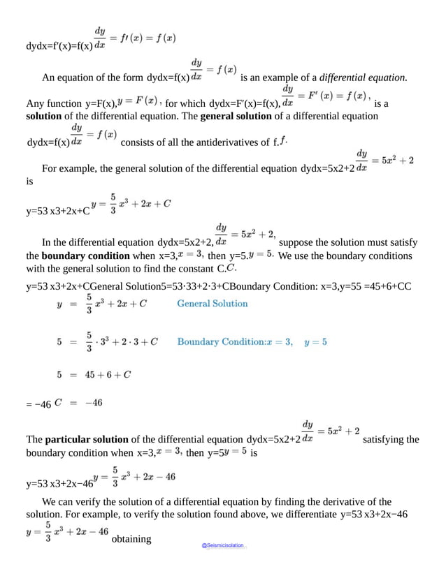
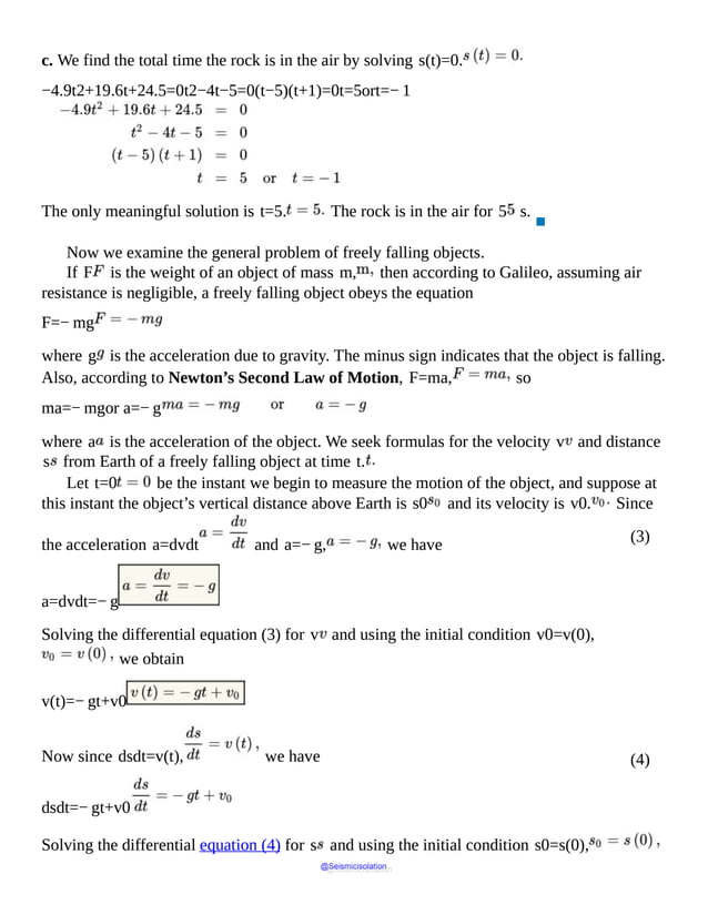
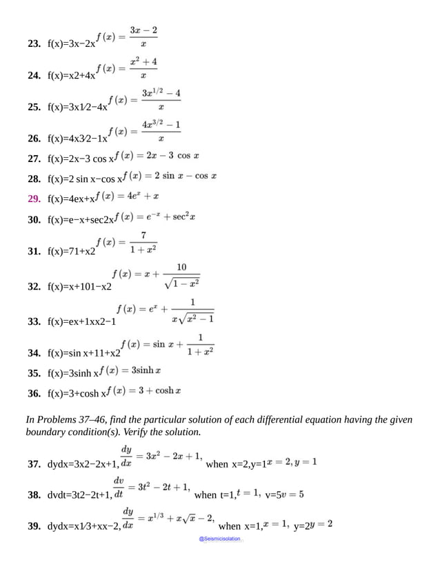
961. Chapter Review
Things to Know
4.1 Related Rates
Steps for solving a related rate problem (p. 264)
4.2 Maximum and Minimum Values; Critical Numbers
Definitions:
Absolute maximum; absolute minimum (p. 272)
Absolute maximum value; absolute minimum value (p. 272)
Local maximum; local minimum (p. 272)
Local maximum value; local minimum value (p. 272)
Critical number (p. 275)
Theorems:
Extreme Value Theorem If a function f is continuous on a closed interval [a,b],
then f has an absolute maximum and an absolute minimum on [a,b]. (p.
274)
If a function f has a local maximum or a local minimum at the number c, then
either f′(c)=0 or f′(c) does not exist. (p. 274)
Procedure:
Steps for finding the absolute extreme values of a function f that is continuous on a
closed interval [a,b]. (p. 277)
4.3 The Mean Value Theorem
Rolle’s Theorem (p. 284)
Mean Value Theorem (p. 285)
Corollaries to the Mean Value Theorem
If f′(x)=0 for all numbers x in (a,b), then f is constant on (a,b).
(p. 287)
If f′(x)=g′(x) for all numbers x in (a,b), then there is a number
C for which f(x)=g(x)+C on(a,b). (p. 288)
Increasing/Decreasing Function Test (p. 288)
4.4 Local Extrema and Concavity
@Seismicisolation
@Seismicisolation

962. Definitions:
Concave up; concave down (p. 299)
Inflection point (p. 300)
Theorems:
First Derivative Test (p. 294)
Test for concavity (p. 299)
A condition for an inflection point (p. 301)
Second Derivative Test (p. 303)
Procedure:
Steps for finding the inflection points of a function (p. 301)
4.5 Indeterminate Forms and L’Hôpital’s Rule
Definitions:
Indeterminate form at c of the type 00 or the type ∞∞ (p. 311)
Indeterminate form at c of the type 0⋅∞ or ∞−∞ (pp. 315–316)
Indeterminate form at c of the type 1∞, 00, or ∞0 (p. 317)
Theorem:
L’Hôpital’s Rule (p. 312)
Procedures:
Steps for finding a limit using L’Hôpital’s Rule (p. 312)
Steps for finding limx→c [f(x)]g(x), where [f(x)]g(x) is an
indeterminate form at c of the type 1∞, 00, or ∞0 (p. 317)
4.6 Using Calculus to Graph Functions
Procedure:
Steps for graphing a function y=f(x). (p. 321)
4.7 Optimization
Procedure:
Steps for solving optimization problems (p. 332)
4.8 Antiderivatives; Differential Equations
Definitions:
Antiderivative (p. 342)
General solution of a differential equation (p. 345)
@Seismicisolation
@Seismicisolation

963. Particular solution of a differential equation (p. 345)
Boundary condition (p. 345)
Initial condition (p. 347)
Basic Antiderivatives See Table 6 (p. 344)
Antidifferentiation Properties:
Sum Rule and Difference Rule: If functions F1 and F2 are antiderivatives of the
functions f1 and f2, respectively, then F1+F2 is an antiderivative of
f1+f2 and F1−F2 is an antiderivative of f1−f2. (p. 344)
Constant Multiple Rule: If k is a real number and if F is an antiderivative of f,
then kF is an antiderivative of kf. (p. 344)
Theorems:
If a function F is an antiderivative of a function f on an interval I, then any other
antiderivative of f has the form F(x)+C, where C is an (arbitrary)
constant. (p. 343)
Newton’s First Law of Motion (p. 351)
Newton’s Second Law of Motion (p. 350)
Objectives
Section You should be able to … Examples Review Exercises
4.1 1 Solve related rate problems (p. 263) 1–5 1–3
4.2
1 Identify absolute maximum and minimum
values and local
1 4, 5
extreme values of a function (p. 272)
2 Find critical numbers (p. 275) 2 6a, 7
3 Find absolute maximum and absolute minimum
values (p. 276)
3–6 8, 9
4.3 1 Use Rolle’s Theorem (p. 284) 1 10
2 Work with the Mean Value Theorem (p. 285) 2, 3 11, 12, 28
3 Identify where a function is increasing and
decreasing (p. 288)
4–7 23a, 24a
4.4
1 Use the First Derivative Test to find local
extrema (p. 294)
1, 2, 3 6b, 13a–15a
2 Use the First Derivative Test with rectilinear
motion (p. 297)
4 16
3 Determine the concavity of a function (p. 298) 5, 6 23b, 24b
4 Find inflection points (p. 300) 7 23c, 24c
5 Use the Second Derivative Test to find local
extrema (p. 302)
8, 9 13b–15b
4.5
1 Identify indeterminate forms of the type 00
1 41–44
@Seismicisolation
@Seismicisolation

964. and ∞∞ (p. 310)
2 Use L’Hôpital’s Rule to find a limit (p. 312) 2–6 45, 47, 49–52, 55
3 Find the limit of an indeterminate form of the 7–10 46, 48, 53, 54, 56
type 0⋅∞,∞−∞, 00,
1∞, or ∞0 (p. 315)
4.6 1 Graph a function using calculus (p. 320) 1–7 17–22, 25, 26, 27
4.7 1 Solve optimization problems (p. 332) 1–6 29, 30, 61–63
4.8 1 Find antiderivatives (p. 342) 1, 2 31–38
2 Solve a differential equation (p. 345) 3, 4 57–60
3 Solve applied problems modeled by differential
equations (p. 347)
5–7 39, 40, 64
Review Exercises
1. Related rates A spherical snowball is melting at the rate of 2 cm3 ⁄min.
How fast is the surface area changing when the radius is 5 cm?
2. Related rates A lighthouse is 3 km from a straight shoreline. Its light makes one
revolution every 8 s. How fast is the light moving along the shore when it makes an
angle of 30 ∘ with the shoreline?
3. Related rates Two planes at the same altitude are approaching an airport, one from the
north and one from the west. The plane from the north is flying at 250mi⁄h
and is 30 mi from the airport. The plane from the west is flying at 200 mi⁄h
and is 20 mi from the airport. How fast are the planes approaching each other at that
instant?
In Problems 4 and 5, use the graphs below to determine whether each function has an
absolute extremum and/or a local extremum or neither at the indicated points.
4.
@Seismicisolation
@Seismicisolation

965. 5.
6. Critical Numbers f(x)=x22x−1
a. Find all the critical numbers of f.
b. Find the local extrema of f.
7. Critical Numbers Find all the critical numbers of f(x)= cos (2x) on
the closed interval [0,π].
In Problems 8 and 9, find the absolute maximum value and absolute minimum value of each
function on the indicated interval.
8. f(x)=x−sin (2x) on [0,2π]
9. f(x)= 32 x4−2x3−6x2+5 on [−2,3]
10. Rolle’s Theorem Verify that the hypotheses for Rolle’s Theorem are satisfied for the
function f(x)=x3−4x2+4x on the interval [0,2]. Find the
coordinates of the point(s) at which there is a horizontal tangent line to the graph of f.
11. Mean Value Theorem Verify that the hypotheses for the Mean Value Theorem are
satisfied for the function f(x)=2x−1x on the interval [1,4]. Find a
point on the graph of f that has a tangent line whose slope equals the slope of the
secant line joining (1,1) to 4,74.
12. Mean Value Theorem Does the Mean Value Theorem apply to the function f(x)=x
@Seismicisolation
@Seismicisolation

966. on the interval [0,9]? If not, why not? If so, find the number c
referred to in the theorem.
In Problems 13–15, find the local extrema of each function:
a. Using the First Derivative Test.
b. Using the Second Derivative Test, if possible. If the Second Derivative Test cannot be
used, explain why.
13. f(x)=x3−x2−8x+1
14. f(x)=x2−24x2⁄3
15. f(x)=x4e−2x
16. Rectilinear Motion The position s of an object from the origin at time t is given by
s=s(t)=t4+2t3−36t2. Draw figures to illustrate the motion of
the object and its velocity.
In Problems 17–22, graph each function. Follow the steps given in Section 4.6.
17. f(x)=−x3−x2+2x
18. f(x)=x1⁄3(x2−9)
19. f(x)=xex
20. f(x)=x−3x2−4
21. f(x)=xx−3
22. f(x)=x3−3ln x
In Problems 23 and 24, for each function :
a. Determine the intervals where each function is increasing and decreasing.
b. Determine the intervals on which each function f is concave up and concave down.
c. Identify any inflection points.
23. f(x)=x4+12x2+36x−11
24. f(x)=3x4−2x3−24x2−7x+2
25. If y is a function and y′>0 for all x and y′′<0 for all x, which of the
@Seismicisolation
@Seismicisolation

967. following could be part of the graph of y=f(x)? See illustrations (A) through
(D).
26. Graph a function f that has the following properties:
f(−3)=2; f(−1)=−5; f(2)=−4;
f(6)=−1; f′(−3)=f′(6)=0;
limx→0− f(x)=−∞; limx→0+ f(x)=∞;
f′′(x)>0 if x<−3 or 0<x<4;
f′′(x)<0 if −3<x<0 or 4<x
27. Graph a function f that has the following properties:
f(−2)=2; f(5)=1; f(0)=0;
f′(x)>0 if x<−2 or 5<x;
f′(x)<0 if −2<x<2 or 2<x<5;
f′′(x)>0 if x<0 or 2<x and f′′(x)<0 if 0<x<2;
limx→2− f(x)=−∞; limx→2+ f(x)=∞
28. Mean Value Theorem For the function f(x)=xx+1, 0≤x≤b,
the number c satisfying the Mean Value Theorem is c=3. Find b.
29. Maximizing Volume An open box is to be made from a piece of cardboard by cutting
@Seismicisolation
@Seismicisolation

968. squares out of each corner and folding up the sides. If the size of the cardboard is 2 ft
by 3 ft, what size squares (in inches) should be cut out to maximize the volume of
the box?
30. Minimizing Distance Find the point on the graph of 2y=x2 nearest to the point
(4,1).
In Problems 31–38, find all the antiderivatives of each function.
31. f(x)=0
32. f(x)=x1⁄2
33. f(x)=cos x
34. f(x)=sec x tan x
35. f(x)=2x
36. f(x)=−2x−3
37. f(x)=4x3−9x2+10x−3
38. f(x)=ex+4x
39. Velocity A box moves down an inclined plane with an acceleration a(t)= t2(t
−3)cm⁄s2. It covers a distance of 10 cm in 2 s. What was the
original velocity of the box?
40. Free Fall Two objects begin a free fall from rest at the same height 1 s apart. How
long after the first object begins to fall will the two objects be 10 m apart?
In Problems 41–44, determine if the expression is an indeterminate form at 0 . If it is,
@Seismicisolation
@Seismicisolation

969. identify its type.
41. xe3x−x1− cos (2x)
42. 1xtan x
43. 1x2−1x2sec x
44. tan x−xx−sin x
In Problems 45–56, find each limit.
45. limx→π⁄2 sec2 xsec2(3x)
46. limx→0 2sin2 x−11−cos x
47. limx→0 ex−e−xsin x
48. limx→0− xcotπx
49. limx→0 tan x +sec x−1tan x −sec x+1
50. limx→a ax−x2a4−2a3x+2ax3−x4
51. limx→0 x−sin xx3
52. limx→0 tan x−sin xsin3 x
53. limx→∞ (1+4x)2⁄x
54. limx→1 [2x2−1−1x−1]
@Seismicisolation
@Seismicisolation

970. 55. limx→4 x2−16x2+x−20
56. limx→0+ (cotx)x
In Problems 57–60, find the particular solution of each differential equation having the given
boundary conditions. Verify the solution.
57. dydx=ex, when x=0, y=2
58. dydx=12 sec x tan x, when x=0, y=7
59. dydx=2x, when x=1, then y=4
60. d2ydx2=x2−4, when x=3, y=2, when x=2, y=2
61. Maximizing Profit A manufacturer has determined that the cost C of producing x
items is given by
C(x)=200+35x+0.02x2 dollars
Each item produced can be sold for $78. How many items should she produce to
maximize profit?
62. Optimization The sales of a new sound system over a period of time are expected to
follow the logistic curve
f(x)= 50001+5e−xx≥0
where x is measured in years. In what year is the sales rate a maximum?
63. Maximum Area Find the area of the rectangle of largest area in the fourth quadrant that
has vertices at (0,0), (x,0), x>0, and (0,y), y<0. The
fourth vertex is on the graph of y=ln x.
64. Differential Equation A motorcycle accelerates at a constant rate from 0 to 72 km⁄h
in 10 s. How far has it traveled in that time?
@Seismicisolation
@Seismicisolation

971. CHAPTER 4 PROJECT The U.S. Economy
Economic data are quite variable and very complicated, making them difficult to model.
The models we use here are rough approximations of the Unemployment Rate and Gross
Domestic Product (GDP).
The unemployment rate can be modeled by
U=U(t)=5 cos 2tπ2+sin 2tπ+60≤t≤25
where t is in years and t=0 represents January 1, 1985.
The GDP growth rate can be modeled by
G=G(t)=5 cos 2tπ+5+20≤t≤25
where t is in years and t=0 represents January 1, 1985. If the GDP growth rate is
increasing, the economy is expanding and if it is decreasing, the economy is contracting.
A recession occurs when GDP growth rate is negative.
1. During what years was the U.S. economy in recession?
@Seismicisolation
@Seismicisolation

972. 2. Find the critical numbers of U=U(t).
3. Determine the intervals on which U is increasing and on which it is decreasing.
4. Find all the local extrema of U.
5. Find the critical numbers of G=G(t).
6. Determine the intervals on which G is increasing and on which it is decreasing.
7. Find all the local extrema of G.
8. a. Find the inflection points of G.
b. Describe in economic terms what the inflection points of G represent.
9. Graph U=U(t) and G=G(t) on the same set of coordinate axes.
10. Okun’s Law states that an increase in the unemployment rate tends to coincide with a
decrease in the GDP growth rate.
a. During years of recession, what is happening to the unemployment rate? Explain
in economic terms why this makes sense.
b. Use your answer to part (a) to explain whether the functions U and G
generally agree with Okun’s Law.
c. If there are times when the functions do not satisfy Okun’s Law, provide an
explanation in economic terms for this.
11. What relationship, if any, exists between the inflection points of the GDP growth rate
and the increase/decrease of the unemployment rate? Explain in economic terms why
such a relationship makes sense.
12. One school of economic thought holds the view that when the economy improves
(increasing GDP), more jobs are created, resulting in a lower unemployment rate.
Others argue that once the unemployment rate improves (decreases), more people are
working and this increases GDP. Based on your analysis of the graphs of U and G,
which position do you support?
______________
For real data on the unemployment rate and GDP, see http://data.bls.gov and
http://www.tradingeconomics.com/united-states/gdp-growth
To read Arthur Okun’s paper, see http://cowles.econ.yale.edu/P/cp/p01b/p0190.pdf
@Seismicisolation
@Seismicisolation

973. 5 The Integral
5.1 Area
5.2 The Definite Integral
5.3 The Fundamental Theorem of Calculus
5.4 Properties of the Definite Integral
5.5 The Indefinite Integral; Method of Substitution
5.6 Separable First-Order Differential Equations; Uninhibited and Inhibited Growth and Decay Models
Chapter Review
Chapter Project
Managing the Klamath River
The Klamath River starts in the eastern lava plateaus of Oregon, passes through a
farming region of that state, and then crosses northern California. Because it is the
largest river in the region, runs through a variety of terrain, and has different land
uses. Historically, the Klamath supported large salmon runs. Now it is used to
irrigate agricultural lands and to generate electric power for the region.
Downstream, it runs through federal wild lands and is used for fishing, rafting, and
kayaking.
@Seismicisolation
@Seismicisolation

974. If a river is to be well-managed for such a variety of uses, its flow must be
understood. For that reason, the U.S. Geological Survey (USGS) maintains a
number of gauges along the Klamath. These typically measure the depth of the
river, which can then be expressed as a rate of flow in cubic feet per second (ft3⁄s
). In order to understand the river flow fully, we must be able to find the total
amount of water that flows down the river over any period of time.
CHAPTER 5 PROJECT The Chapter Project on page 426 examines ways to
obtain the total flow of a river over any period of time from data that provide flow
rates.
We began our study of calculus by asking two questions from geometry. The first, the
tangent problem, “What is the slope of the tangent line to the graph of a function?" led to the
derivative of a function.
The second question was the area problem, “Given a function f, defined and
nonnegative on a closed interval [a,b], what is the area of the region enclosed by the
graph of f, the x -axis, and the vertical lines x=a and x=b ?” Figure 1
illustrates this region. Answering the area problem question leads to the integral of a
function.
Figure 1 A is the area of the region enclosed by the graph of f, the x -axis, and the
lines x=a and x=b.
It
shows
a
shaded
area
The first two sections of Chapter 5 show how the concept of the integral evolves from the
area problem. At first glance, the area problem and the tangent problem look quite dissimilar.
However, much of calculus is built on a surprising relationship between the two problems
and their associated concepts. This relationship is the basis for the Fundamental Theorem of
Calculus, discussed in Section 5.3.
@Seismicisolation
@Seismicisolation

975. 5.1 Area
OBJECTIVES When you finish this section, you should be able to:
1 Approximate the area under the graph of a function
2 Find the area under the graph of a function
The area problem asks, “Given a function f, defined and nonnegative on a closed interval
[a,b], what is the area A of the region enclosed by the graph of f, the x -axis, and
the vertical lines x=a and x=b ?” To answer the question posed in the area
problem, we approximate the area A of the region by adding the areas of a finite number of
rectangles, as shown in Figure 2. This approximation of the area A will lead to the integral,
which gives the exact area A of the region. We begin by reviewing the formula for the area
of a rectangle.
Figure 2 The sum of the areas of the rectangles approximates the area of the region.
It
shows
a
shaded
area
A
equal
to
sum
of
finite
The area A of a rectangle with width w and height h is given by the geometry
formula
A=hw
See Figure 3. The graph of a constant function f(x)=h, for some positive
number h, is a horizontal line that lies above the x -axis. The region enclosed by this line,
the x -axis, and the lines x=a and x=b is the rectangle whose area A is the
product of the width (b−a) and the height h.
A=h(b−a)
@Seismicisolation
@Seismicisolation

976. Figure 3 A=h(b−a).
It
shows
a
shaded
area
A
equal
to
area
of
rectangle
with
height
h
and
width
b
minus
a,
under
the
curve
depicting
function
f
of
x
and
If the graph of y=f(x) consists of three horizontal lines, each of positive height
as shown in Figure 4, the area A enclosed by the graph of f, the x -axis, and the lines
x=a and x=b is the sum of the rectangular areas A1, A2, and A3.
Figure 4 A=A1+A2+A3
It
shows
a
shaded
area
A
equal
to
sum
of
areas
of
1 Approximate the Area Under the Graph of a Function
EXAMPLE 1 Approximating the Area Under the Graph of a Function
Approximate the area A of the region enclosed by the graph of f(x)=12 x+3,
the x -axis, and the lines x=2 and x=4.
Solution Figure 5 illustrates the area A to be approximated.
@Seismicisolation
@Seismicisolation

977. Figure 5
It
shows
shaded
area
A
under
the
line
depicting
function
f
of
x
and
bounded
by
x
axis
and
the
vertical
lines
x
equal
We begin by drawing a rectangle of width 4−2=2 and height f(2)=4.
The area of the rectangle, 2⋅4=8, approximates the area A, but it underestimates
A, as seen in Figure 6(a).
Figure 6
It
Alternatively, A can be approximated by a rectangle of width 4−2=2 and
height f(4)=5. See Figure 6(b). This approximation of the area equals 2⋅5=10,
@Seismicisolation
@Seismicisolation

978. but it overestimates A. We conclude that
8<A<10
The approximation of the area A of the region can be improved by dividing the closed
interval [2,4] into two subintervals, [2,3] and [3,4]. Now draw two
rectangles: one rectangle with width 3−2=1 and height f(2)=12⋅2+3=4
; the other rectangle with width 4−3=1 and height
f(3)=12⋅3+3=92. As Figure 7(a) illustrates, the sum of the areas of the
two rectangles
1⋅4+1⋅92=172=8.5
underestimates the area.
Figure 7
Repeat this process by drawing two rectangles, one of width 1 and height f(3)=92;
the other of width 1 and height f(4)=12⋅4+3=5. The sum
of the areas of these two rectangles,
1⋅92+1⋅5=192=9.5
@Seismicisolation
@Seismicisolation

979. overestimates the area as shown in Figure 7(b). We conclude that
8.5<A<9.5
obtaining a better approximation to the area.
▪
Observe that as the number n of subintervals of the interval [2,4 ] increases, the
approximation of the area A improves. For n=1, the error in approximating A is 1
square unit, but for n=2, the error is only 0.5 square unit.
NOTE The actual area in Figure 5 is 9 square units, obtained by using the formula for the area A of a
trapezoid with base b and parallel heights h1 and h2:
A=12 b(h1+h2)=12 (2)(4+5)=9.
NOW WORK Problem 5.
In general, the procedure for approximating the area A is based on the idea of summing
the areas of rectangles. We shall refer to the area A of the region enclosed by the graph of a
function y=f(x)≥0, the x -axis, and the lines x=a and x=b as the
area under the graph of f from a to b.
We make two assumptions about the function f :
f is continuous on the closed interval [a,b].
f is nonnegative on the closed interval [a,b].
We divide, or partition, the interval [a,b] into n nonoverlapping subintervals:
[x0,x1],[x1,x2],…,[xi−1,xi],…,[xn−1,xn]x0=a,xn=b
each of the same length. See Figure 8. Since there are n subintervals and the length of the
interval [a,b] is b−a, the common length Δx of each subinterval is
Δx=b−an
@Seismicisolation
@Seismicisolation

980. Figure 8
The
number
line
is
divided
into
n
partitions
with
length
of
each
partition
equal
to
delta
x.
Since f is continuous on the closed interval [a,b], it is continuous on every
subinterval [xi−1,xi] of [a,b]. By the Extreme Value Theorem, there is a
number in each subinterval where f attains its absolute minimum. Label these numbers c1,
c2, c3,…,cn, so that f(ci) is the absolute minimum value of f in the
subinterval [xi−1,xi]. Now construct n rectangles, each having Δx as its base
and f(ci) as its height, as illustrated in Figure 9. This produces n narrow rectangles of
uniform width Δx=b−an and heights f(c1),f(c2),…,f(cn),
respectively. The areas of the n rectangles are
Areaofthefirstrectangle=f(c1)ΔxAreaofthesecondrectangle=f(c2)Δx⋮Areaofthenth(andlast)rectangle
Figure 9 f(ci) is the absolute minimum value of f on [xi−1,xi].
It
shows
NEED TO REVIEW? The Extreme Value Theorem is discussed in Section 4.2, p. 274.
@Seismicisolation
@Seismicisolation

981. The sum sn of the areas of the n rectangles approximates the area A. That is,
A≈sn=f(c1)Δx+f(c2)Δx+⋯+f(ci)Δx+⋯+f(cn)Δx=∑i=1nf(ci)Δx
Since the rectangles used to approximate the area A lie under the graph of f, the sum sn,
called a lower sum, underestimates A. That is, sn≤A.
NEED TO REVIEW? Summation notation is discussed in Section P.8, pp. 71–72.
EXAMPLE 2 Approximating Area Using Lower Sums
Approximate the area A under the graph of f(x)=x2 from 0 to 10 by using
lower sums sn (rectangles that lie under the graph) for:
a. n=2 subintervals
b. n=5 subintervals
c. n=10 subintervals
Solution a. For n=2, we partition the closed interval [0,10] into two
subintervals [0,5] and [5,10], each of length Δx=10−02=5.
See Figure 10(a). To compute s2, we need to know where f attains its minimum value in
each subinterval. Since f is an increasing function on [0,10 ], the absolute minimum is
attained at the left endpoint of each subinterval. So, for n=2, the minimum of f on
[0,5] occurs at 0 and the minimum of f on [5,10] occurs at 5. The lower sum
s2 is
@Seismicisolation
@Seismicisolation

982. Figure 10
b. For n=5, partition the interval [0,10] into five subintervals [0,2], [2,4],
[4,6], [6,8], [8,10], each of length Δx=10−05=2.
See Figure 10(b). The lower sum s5 is
s5=∑i=15 f(ci)Δx=Δx∑i=15f(ci)=2[f(0)+f(2)+f(4)+f(6)+f(8)]=2(0+4+16+36+64)=240
c. For n=10, partition [0,10] into 10 subintervals, each of length
Δx=10−010=1. See Figure 10(c). The lower sum s10 is
s10=∑i=110 f(ci)Δx ​= ​Δx∑i=110f(ci) ​=​
1[f(0)​+​f(1)​+​f(2)​+...+​f(9)]=0+1+4+9+16+25+36+49+64+81=​285
▪
NOW WORK Problem 13(a).
In general, as Figure 11(a) illustrates, the error due to using lower sums sn (rectangles
that lie below the graph of f ) occurs because a portion of the region lies outside the
rectangles. To improve the approximation of the area, we increase the number of
subintervals. For example, in Figure 11(b), there are four subintervals and the error is
@Seismicisolation
@Seismicisolation

983. reduced; in Figure 11(c), there are eight subintervals and the error is further reduced. By
taking a finer and finer partition of the interval [a,b], that is, by increasing the number
n of subintervals without bound, we can make the sum of the areas of the rectangles as
close as we please to the actual area of the region. (A proof of this statement is usually found
in books on advanced calculus.)
Figure 11
For functions that are continuous on a closed interval, limn→∞sn always exists.
With this in mind, we now define the area under the graph of a function f from a to b.
DEFINITION Area A Under the Graph of a Function from a to b
Suppose a function f is nonnegative and continuous on a closed interval [a,b].
Partition [a,b] into n subintervals [x0,x1],[x1,x2],…,[xi−1,xi],…,[xn−1,xn],
each of length
Δx=b−an
In each subinterval [xi−1,xi], let f(ci) equal the absolute minimum value of
f on the subinterval. Form the lower sums
sn=∑i=1nf(ci)Δx=f(c1)Δx+⋯+f(cn)Δx
The area A under the graph of f from a to b is the number
A=limn→∞sn
@Seismicisolation
@Seismicisolation

984. The area A is defined using lower sums sn (rectangles that lie below the graph of f
). By a parallel argument, we can choose values C1,C2,…,Cn so that the
height f(Ci) of the i th rectangle is the absolute maximum value of f on the i th
subinterval, as shown in Figure 12. The corresponding upper sums Sn (rectangles that
extend above the graph of f ) overestimate the area A. So, Sn≥A. It can be shown
that as n increases without bound, the limit of the upper sums Sn equals the limit of the
lower sums sn. That is,
limn→∞sn=limn→∞Sn=A
Figure 12 f(Ci) is the absolute maximum value of f on [xi−1,xi].
NOW WORK Problem 13(b).
2 Find the Area Under the Graph of a Function
In the next example, instead of using a specific number of rectangles to approximate area, we
partition the interval [a,b] into n subintervals, obtaining n rectangles. By letting
n→∞, we find the actual area under the graph of f from a to b.
EXAMPLE 3 Finding Area Using Upper Sums
Find the area A under the graph of f(x)=3x from 0 to 10 using upper sums
Sn (rectangles that extend above the graph of f). That is, find A=limn→∞Sn.
Solution Figure 13 illustrates the area A. Partition the closed interval [0,10] into n
subintervals
@Seismicisolation
@Seismicisolation

985. [x0,x1],[x1,x2],…,[xi−1,xi],…,[xn−1,xn]
where
0=x0<x1<x2<⋯<xi<⋯<xn−1<xn=10
and each subinterval is of length
Δx=10−0n=10n
As illustrated in Figure 14, coordinates of the endpoints of each subinterval, written in terms
of n, are
x0=0,x1=10n,x2=210n,…,xi−1=(i−1)10n,xi=i10n,…,xn=n10n=10
Figure 13 f(x)=3x,0≤x≤10
@Seismicisolation
@Seismicisolation

986. Figure 14
To find A using upper sums Sn (rectangles that extend above the graph of f), we
need the absolute maximum value of f in each subinterval. Since f(x)=3x is an
increasing function, the absolute maximum occurs at the right endpoint xi=i10n=10in
of each subinterval. So, Ci=xi, f(Ci)=3xi, and
Using summation properties, we get
Sn=∑i=1n300n2 i=300n2∑i=1ni=300n2⋅n(n+1)2=150n+1n=1501+1n
NEED TO REVIEW? Summation properties are discussed in Section P.8, pp. 72–73.
RECALL ∑i=1ni=n(n+1)2 (p. 72)
Then
A=limn→∞Sn=limn→∞1501+1n=150limn→∞1+1n=150
The area A under the graph of f(x)=3x from 0 to 10 is 150 square units.
▪
@Seismicisolation
@Seismicisolation

987. NOTE The region under the graph of f(x)=3x from 0 to 10 is a triangle. So, we can
verify that A=150 by using the formula for the area A of a triangle with base b
and height h :
A=12 bh=12 (10)(30)=150
EXAMPLE 4 Finding Area Using Lower Sums
Find the area A under the graph of f(x)=16−x2 from 0 to 4 by using
lower sums sn (rectangles that lie below the graph of f ). That is, find A=limn→∞sn.
Solution Figure 15 shows the area under the graph of f and a typical rectangle that lies
below the graph. Partition the closed interval [0,4] into n subintervals
[x0,x1],[x1,x2],…,[xi−1,xi],…,[xn−1,xn]
where
0=x0<x1<⋯<xi<⋯<xn−1<xn=4
and each interval is of length
Δx=4−0n=4n
As Figure 16 illustrates, the endpoints of each subinterval, written in terms of n, are
x0=0,x1=14n,x2=24n,…,xi−1=(i−1)4n,xi=i 4n,…,xn=n4n=4
@Seismicisolation
@Seismicisolation

988. Figure 15 f(x)=16−x2,0≤x≤4
It
shows
a
shaded
area
A
under
the
curve
depicting
function
f
of
x
for
x
equal
to
0
and
x
equal
to
Figure 16
To find A using lower sums sn (rectangles that lie below the graph of f ), we must
find the absolute minimum value of f on each subinterval. Since the function f is a
decreasing function, the absolute minimum occurs at the right endpoint of each subinterval.
Since ci=i4n=4in and Δx=4n,
(ci)Δx=∑i=1n 16−4in24nci=4in;f(ci)=16−ci2;Δx=4n=∑i=1n 64n
64n∑i=1n1−64n3∑i=1ni2=64n (n)−64n3 n(n+1)(2n+1)6=64−323n2 2n2+3n+1=64−643−32n
1283−32n−323n2
RECALL ∑i=1n1=n ∑i=1ni2=n(n+1)(2n+1)6 (p. 72)
@Seismicisolation
@Seismicisolation

989. Then
A=limn→∞ sn=limn→∞1283−32n−323n2=1283
The area A under the graph of f(x)=16−x2 from 0 to 4 is 1283
square units. ▪
NOW WORK Problem 29.
The previous two examples illustrate just how complex it can be to find areas using lower
sums and/or upper sums. In the next section, we define an integral and show how it can be
used to find area. Then in Section 5.3, we present the Fundamental Theorem of Calculus,
which provides a relatively simple way to find area.
5.1 Assess Your Understanding
Concepts and Vocabulary
1. Explain how rectangles can be used to approximate the area of the region enclosed by
the graph of a function y=f(x)≥0, the x -axis, and the lines x=a and
x=b.
2. True or False When a closed interval [a,b] is partitioned into n subintervals each
of the same length, the length of each subinterval is a+bn.
3. If the closed interval [−2,4] is partitioned into 12 subintervals, each of the
same length, then the length of each subinterval is ______.
4. True or False If the area A under the graph of a function f that is continuous and
nonnegative on a closed interval [a,b] is approximated using upper sums Sn,
then Sn≥A and A=limn→∞Sn.
Skill Building
5. Approximate the area A of the region enclosed by the graph of f(x)=12 x+3,
the x -axis, and the lines x=2 and x=4 by partitioning the
closed interval [2,4] into four subintervals:
@Seismicisolation
@Seismicisolation

990. 2,52, 52,3, 3,72, 72,4
a. Using the left endpoint of each subinterval, draw four small rectangles that lie
below the graph of f and sum the areas of the four rectangles.
b. Using the right endpoint of each subinterval, draw four small rectangles that extend
above the graph of f and sum the areas of the four rectangles.
c. Compare the answers from parts (a) and (b) to the exact area A=9 and to the
estimates obtained in Example 1.
6. Approximate the area A of the region enclosed by the graph of f(x)=6−2x,
the x -axis, and the lines x=1 and x=3 by partitioning the
closed interval [1,3] into four subintervals:
1,32, 32,2,2,52,52,3
a. Using the right endpoint of each subinterval, draw four small rectangles that lie
below the graph of f and sum the areas of the four rectangles.
b. Using the left endpoint of each subinterval, draw four small rectangles that extend
above the graph of f and sum the areas of the four rectangles.
c. Compare the answers from parts (a) and (b) to the exact area A=4.
In Problems 7 and 8, refer to the graphs below. Approximate the shaded area under the
graph of f :
a. By constructing rectangles using the left endpoint of each subinterval.
b. By constructing rectangles using the right endpoint of each subinterval.
@Seismicisolation
@Seismicisolation

991. 7.
8.
In Problems 9–12, partition each interval into n subintervals each of the same length.
9. [1,4] with n=3
10. [0,9] with n=9
11. [−1,4] with n=10
12. [−4,4] with n=16
In Problems 13 and 14, refer to the graphs. Using the indicated subintervals, approximate
the shaded area:
a. By using lower sums sn (rectangles that lie below the graph of f ).
b. By using upper sums Sn (rectangles that extend above the graph of f ).
@Seismicisolation
@Seismicisolation

992. 13.
14.
15. Area Under a Graph
a. Graph y=x and indicate the area under the graph from 0 to 3.
b. Partition the interval [0,3] into n subintervals each of equal length.
c. Show that sn=∑i=1n(i−1) 3n2.
d. Show that Sn=∑i=1ni 3n2.
e. Show that limn→∞ sn=limn→∞Sn=92.
16. Area Under a Graph
@Seismicisolation
@Seismicisolation

993. a. Graph y=4x and indicate the area under the graph from 0 to 5.
b. Partition the interval [0,5] into n subintervals each of equal length.
c. Show that sn=∑i=1n(i−1)100n2.
d. Show that Sn=∑i=1ni 100n2.
e. Show that limn→∞ sn=limn→∞ Sn=50.
In Problems 17–22, approximate the area A under the graph of each function f from a
to b for n=4 and n=8 subintervals:
a. By using lower sums sn (rectangles that lie below the graph of f ).
b. By using upper sums Sn (rectangles that extend above the graph of f ).
17. f(x)=−x+10 on [0,8]
18. f(x)=2x+5 on [2,6]
19. f(x)=16−x2 on [0,4]
20. f(x)=x3 on [0,8]
21. f(x)=cos x on −π2,π2
22. f(x)=sin x on [0,π]
23. Rework Example 3 (p. 362) by using lower sums sn (rectangles that lie below the
graph of f ).
24. Rework Example 4 (p. 363) by using upper sums Sn (rectangles that extend above
the graph of f ).
In Problems 25–32, find the area A under the graph of f from a to b :
a. By using lower sums sn (rectangles that lie below the graph of f ).
b. By using upper sums Sn (rectangles that extend above the graph of f ).
c. Compare the work required in (a) and (b). Which is easier? Could you have predicted
this?
25. f(x)=2x+1 from a=0 to b=4
@Seismicisolation
@Seismicisolation

994. 26. f(x)=3x+1 from a=0 to b=4
27. f(x)=12−3x from a=0 to b=4
28. f(x)=5−x from a=0 to b=4
29. f(x)=4x2 from a=0 to b=2
30. f(x)=12 x2 from a=0 to b=3
31. f(x)=4−x2 from a=0 to b=2
32. f(x)=12−x2 from a=0 to b=3
Applications and Extensions
In Problems 33–38, find the area under the graph of f from a to b. Partition the closed
interval [a,b] into n subintervals
[x0,x1],[x1,x2],…,[xi− 1,xi],…,[xn−1,xn],
where a=x0<x1<⋯<xi<⋯<xn−1<xn=b, and
each subinterval is of length Δx=b−an. As the Figure below illustrates, the
endpoints of each subinterval, written in terms of n , are
x0=a,x1=a+b−an,x2=a+2b−an,…,xi−1=a+(i−1)b−an,xi=a+ib−an,…,xn=a+nb−an=b
33. f(x)=x+3 from a=1 to b=3
34. f(x)=3−x from a=1 to b=3
@Seismicisolation
@Seismicisolation

995. 35. f(x)=2x+5 from a=−1 to b=2
36. f(x)=2−3x from a=−2 to b=0
37. f(x)=2x2+1 from a=1 to b=3
38. f(x)=4−x2 from a=1 to b=2
In Problems 39–42, approximate the area A under the graph of each function f by
partitioning [a,b] into 20 subintervals of equal length and using an upper sum.
39. f(x)=xex on [0,8]
40. f(x)=ln x on [1,3]
41. f(x)=1x on [1,5]
42. f(x)=1x2 on [2,6]
43.
a. Graph y=4x from x=1 to x=4 and shade the area under its graph.
b. Partition the interval [1,4] into n subintervals of equal length.
c. Show that the lower sum sn is
sn=∑i=1n41+3in 3n
d. Show that the upper sum Sn is
Sn=∑i=1n41+3(i−1)n 3n
e. Complete the following table:
n 5 10 50 100
sn
Sn
f. Use the table to give an upper and lower bound for the area.
Challenge Problems
@Seismicisolation
@Seismicisolation

996. 44. Area Under a Graph Approximate the area under the graph of f(x)=x from
a≥0 to b by using lower sums sn and upper sums Sn for a partition of [a,b]
into n subintervals, each of length b−an. Show that
sn<b2−a22<Sn
45. Area Under a Graph Approximate thearea under the graph of f(x)=x2 from
a≥0 to b by using lower sums sn and upper sums Sn for a partition of [a,b]
into n subintervals, each of length b−an. Show that
sn<b3−a33<Sn
46. Area of a Right Triangle Use lower sums sn (rectangles that lie inside the triangle)
and upper sums Sn (rectangles that extend outside the triangle) to find the area of a
right triangle of height H and base B.
47. Area of a Trapezoid Use lower sums sn (rectangles that lie inside the trapezoid) and
upper sums Sn (rectangles that extend outside the trapezoid) to find the area of a
trapezoid of heights H1 and H2 and base B.
1. = NOW WORK problem
= Graphing technology recommended
= Computer Algebra System recommended
@Seismicisolation
@Seismicisolation

997. 5.2 The Definite Integral
OBJECTIVES When you finish this section, you should be able to:
1 Form Riemann sums
2 Define a definite integral as the limit of Riemann sums
3 Approximate a definite integral using Riemann sums
4 Know conditions that guarantee a definite integral exists
5 Find a definite integral using the limit of Riemann sums
6 Form Riemann sums from a table
The area A under the graph of y=f(x) from a to b is obtained by finding
A=limn→∞sn=limn→∞∑i=1nf(ci)Δx=limn→∞Sn=limn→∞∑i=1nf(Ci)Δx
where the following assumptions are made:
The function f is continuous on the closed interval [a,b].
The function f is nonnegative on the closed interval [a,b].
The closed interval [a,b] is partitioned into n subintervals, each of length
Δx=b−an
f(ci) is the absolute minimum value of f on the i th subinterval, i=1,2,…,n.
f(Ci) is the absolute maximum value of f on the i th subinterval, i=1,2,…,n.
@Seismicisolation
@Seismicisolation

998. ORIGINS Riemann sums are named after the German mathematician Georg Friedrich Bernhard Riemann
(1826–1866). Early in his life, Riemann was home schooled. At age 14, he was sent to a lyceum (high school)
and then the University of Göttingen to study theology. Once at Göttingen, he asked for and received
permission from his father to study mathematics. He completed his Ph.D. under Karl Friedrich Gauss (1777–
1855). In his thesis, Riemann used topology to analyze complex functions. Later he developed a theory of
geometry to describe real space. His ideas were far ahead of their time and were not truly appreciated until they
provided the mathematical framework for Einstein’s Theory of Relativity.
In Section 5.1, we found the area A under the graph of f from a to b by choosing
either the number ci, where f has an absolute minimum on the i th subinterval, or the
number Ci, where f has an absolute maximum on the i th subinterval. Suppose we
arbitrarily choose a number ui in each subinterval [xi−1,xi], and draw rectangles
of height f(ui) and length Δx. Then from the definitions of absolute minimum
value and absolute maximum value
f(ci)≤f(ui)≤f(Ci)
and, since Δx>0,
f(ci)Δx≤f(ui)Δx≤f(Ci)Δx
Then
∑i=1nf(ci)Δx≤∑i=1nf(ui)Δx≤∑i=1nf(Ci)Δxsn≤∑i=1nf(ui)Δx≤Sn
Since limn→∞sn=limn→∞Sn=A, by the Squeeze Theorem, we have
limn→∞∑i=1nf(ui)Δx=A @Seismicisolation
@Seismicisolation

999. NEED TO REVIEW? The Squeeze Theorem is discussed in Section 1.4, pp. 115–116.
In other words, we can use any number ui in the i th subinterval to find the area A.
1 Form Riemann Sums
We now investigate sums of the form
∑i=1nf(ui)Δxi
using the following more general assumptions:
The function f is defined on a closed interval [a,b].
The function f is not necessarily continuous on [a,b].
The function f is not necessarily nonnegative on [a,b].
The lengths Δxi=xi−xi−1 of the subintervals [xi−1,xi], i=1,2,
…,n of [a,b] are not necessarily equal.
The number ui may be any number in the subinterval [xi−1,xi], i=1,2,…,n.
The sums ∑i=1nf(ui)Δxi, called Riemann sums for f on [a,b], are
the foundation of integral calculus.
EXAMPLE 1 Finding Riemann Sums
For the function f(x)=x2−3, 0≤x≤6, partition the interval [0,6]
into four subintervals [0,1], [1,2], [2,4], [4,6] and find the Riemann
sum for which
a. ui is the left endpoint of each subinterval.
b. ui is the midpoint of each subinterval.
Solution In forming Riemann sums ∑i=1nf(ui)Δxi, n is the number of
subintervals in the partition, f(ui) is the value of f at the number ui chosen in the i
th subinterval, and Δxi is the length of the i th subinterval. The 4 subintervals have
length
@Seismicisolation
@Seismicisolation

1000. Δx1=1−0=1Δx2=2−1=1Δx3=4−2=2Δx4=6−4=2
a. Figure 17 shows the graph of f, the partition of the interval [0,6] into the 4
subintervals, and values of f(ui) at the left endpoint of each subinterval, namely,
f(u1)=f(0)=−3f(u2)=f(1)=−2f(u3)=f(2)=1f(u4)=f(4)=13
The Riemann sum is found by adding the products f(ui)Δxi for i=1,2,3,4.
∑i=14f(ui)Δxi=f(u1)Δx1+f(u2)Δx2+f(u3)Δx3+f(u4)Δx4=−3⋅1+(−2)⋅1+1⋅2+13⋅2=23
Figure 17 f(x)=x2−3,0≤x≤6
b. See Figure 18. If ui is chosen as the midpoint of each subinterval, then the value of f(ui)
at the midpoint of each subinterval is
f(u1)=f12=−114f(u2)=f32=−34f(u3)=f(3)=6f(u4)=f(5)=22
@Seismicisolation
@Seismicisolation

1001. The Riemann sum is found by adding the products f(ui)Δxi for i=1,2,3,4.
∑i=14f(ui)Δxi=f(u1)Δx1+f(u2)Δx2+f(u3)Δx3+f(u4)Δx4=−114⋅1+
−34⋅1+6⋅2+22⋅2=1052=52.5
▪
Figure 18 f(x)=x2−3,0≤x≤6
NOW WORK Problem 9.
2 Define a Definite Integral as the Limit of Riemann Sums
Suppose a function f is defined on a closed interval [a,b], and we partition the interval
[a,b] into n subintervals
[x0,x1],[x1,x2],[x2,x3],…,[xi−1,xi],…,[xn−1,xn]
@Seismicisolation
@Seismicisolation

1002. where
a=x0<x1<x2<⋯<xi−1<xi<⋯<xn−1<xn=b
These subintervals are not necessarily of the same length. Denote the length of the first
subinterval by Δx1=x1−x0, the length of the second subinterval by
Δx2=x2−x1, and so on. In general, the length of the i th subinterval is
Δxi=xi−xi−1
for i=1,2,…,n. This set of subintervals of the interval [a,b] is called a
partition of [a,b]. The length of the largest subinterval in a partition is called the norm
of the partition and is denoted by maxΔxi.
DEFINITION Definite Integral
Let f be a function defined on the closed interval [a,b]. Partition [a,b] into n
subintervals of length Δxi=xi−xi−1, i=1,2,…,n. Choose a
number ui in each subinterval, evaluate f(ui), and form the Riemann sums
∑i=1nf(ui)Δxi. If limmax Δxi→0∑i=1nf(ui) Δxi=I
exists and does not depend on the choice of the partition or on
the choice of ui, then the number I is called the Riemann integral or definite integral
of f from a to b and is denoted by the symbol ∫abf(x)dx. That is,
∫abf(x)dx=limmax Δxi→0∑​i=1nf(ui)Δxi
When the above limit exists, then we say that f is integrable over [a,b] or that
∫abf(x)dx exists.
If f is integrable over [a,b], then limmax Δxi→0 ∑i=1nf(ui) Δxi
exists for any choice of ui in the i th subinterval, so we are free to
choose the ui any way we please. The choices could be the left endpoint of each
@Seismicisolation
@Seismicisolation

1003. subinterval, or the right endpoint, or the midpoint, or any other number in each subinterval.
Also, limmax Δxi→0 ∑i=1nf(ui) Δxi is independent of the partition
of the closed interval [a,b], provided max Δxi can be made as close as we
please to 0. It is this flexibility that makes the definite integral so important in engineering,
physics, chemistry, geometry, and economics.
EXAMPLE 2 Expressing the Limit of Riemann Sums as a Definite Integral
The Riemann sums for f(x)=x2−3 on the closed interval [0,6] are
∑i=1nf(ui)Δxi=∑i=1nui2−3Δxi
where [0,6] is partitioned into n subintervals [xi−1,xi] of length Δxi and
ui is some number in the subinterval [xi−1,xi], i=1,2,…,n.
Assuming that the limit of the Riemann sums exists as max Δxi→0, express
the limit as a definite integral.
Solution Since limmax Δxi→0∑i=1n(ui2−3)Δxi exists, then
limmax Δxi→0∑i=1n(ui2−3)Δxi=∫06(x2−3) dx
▪
NOW WORK Problem 19.
For the definite integral ∫abf(x)dx, the number a is called the lower limit of
integration, the number b is called the upper limit of integration, the symbol ∫ is called
the integral sign, f(x) is called the integrand, and dx is the differential of the
independent variable x. The variable used in the definite integral is an artificial or a
dummy variable because it may be replaced by any other symbol. For example,
∫abf(x)dx∫abf(t)dt∫abf(s)ds∫abf(θ)dθ
all denote the definite integral of f from a to b, and if any one of them exists, they all
exist and equal the same number. @Seismicisolation
@Seismicisolation

1004. NOTE The integral sign ∫ is an elongated “S” to remind you of summation.
EXAMPLE 3 Expressing a Definite Integral as the Limit of Riemann Sums
Express ∫−14(x3−2)dx as the limit of Riemann sums.
Solution The integrand is f(x)=x3−2. The lower limit of integration is −1
and the upper limit of integration is 4, so the interval [−1,4] is partitioned. Partition
the interval [−1,4] into n subintervals of length Δxi,i=1,2,…,n.
Let max Δxi denote the largest of these lengths. If ui is any number in the i th
subinterval, the Riemann sums of f on [−1,4] are
∑i=1nf(ui)Δxi=∑i=1n(ui3−2)Δxi
Then
∫−14 (x3​−​2)​dx​=limmax Δxi→0∑i=1n(ui3−2)Δxi
▪
NOW WORK Problem 33.
In defining the definite integral ∫abf(x)dx, we assumed that a<b. To
remove this restriction, we give the following definitions.
DEFINITION
If f(a) is defined, then
∫aaf(x)dx=0
(2)
If a>b and if ∫baf(x)dx exists, then
∫abf(x)dx=−∫baf(x)dx
(3)
@Seismicisolation
@Seismicisolation

1005. IN WORDS Interchanging the limits of integration reverses the sign of the definite integral.
EXAMPLE 4 Using (2) and (3)
a. ∫11x2dx=0
b. ∫23x2dx=−∫23x2dx
▪
NOW WORK Problem 17.
3 Approximate a Definite Integral Using Riemann Sums
Suppose f is integrable over the closed interval [a,b]. Then
∫​abf(x)​dx​=​limmax Δxi→0∑​i=1nf(ui)Δxi
To approximate ∫abf(x)dx using Riemann sums, we usually partition [a,b]
into n subintervals, each of the same length Δx=b−an. Then Δxi=Δx
for each i=1,2,3,…,n and
∫abf(x)dx≈∑i=1nf(ui)Δx
where ui is usually chosen as the left endpoint, the right endpoint, or the midpoint of the
ith subinterval [xi−1,xi].
EXAMPLE 5 Approximating a Definite Integral Using Riemann Sums
Approximate ∫19(x−3)2dx by partitioning [1,9] into four subintervals each
of length 2
a. using a Left Riemann sum. (Choose ui as the left endpoint of the ith subinterval.)
b. using a Right Riemann sum. (Choose ui as the right endpoint of the ith subinterval.)
@Seismicisolation
@Seismicisolation

1006. c. using a Midpoint Riemann sum. (Choose ui as the midpoint of the ith subinterval.)
NOTE
Riemann sums formed using the left endpoint of each subinterval are called Left Riemann sums.
Riemann sums formed using the midpoint of each subinterval are called Midpoint Riemann sums.
Riemann sums formed using the right endpoint of each subinterval are called Right Riemann sums.
Solution For the given partition Δx=9−14=2 and the four subintervals are
[1,3],[3,5],[5,7],[7,9]
a. We choose ui to be the left endpoint of the ith subinterval. Then u1=1, u2=3,
u3=5, u4=7, and
∫19(x−3)2dx≈∑i=14f(ui)Δx=[f(1)+f(3)+f(5)+f(7)]Δx=[4+0+4+16]⋅2=48
b. We choose ui to be the right endpoint of the ith subinterval. Then u1=3, u2=5,
u3=7, u4=9, and
∫19(x−3)2dx≈∑i=14f(ui)Δx=[f(3)+f(5)+f(7)+f(9)]Δx=[0+4+16+36]⋅2=112
c. We choose ui to be the midpoint of the ith subinterval. Then u1=2, u2=4,
u3=6, u4=8, and
∫19(x−3)2dx≈∑i=14f(ui)Δx=[f(2)+f(4)+f(6)+f(8)]Δx=[1+1+9+25]⋅2=72
▪
NOW WORK Problem 39(a) and (b).
@Seismicisolation
@Seismicisolation

1007. 4 Know Conditions That Guarantee a Definite Integral Exists
Below we state two theorems that give conditions that guarantee a function f is integrable.
The proofs of these two results may be found in advanced calculus texts.
NEED TO REVIEW? Continuity is discussed in Section 1.3, pp. 102–109.
THEOREM Existence of the Definite Integral
If a function f is continuous on a closed interval [a,b], then the definite integral
∫abf(x)dx exists.
IN WORDS If a function f is continuous on [a,b], then it is integrable over [a,b]. But if f is not
continuous on [a,b], then f may or may not be integrable over [a,b].
The hypothesis of the theorem deserves special attention. First, f is defined on a closed
interval, and second, f is continuous on that interval. There are some functions that are
continuous on an open interval (or even a half-open interval) for which the integral does not
exist. Also, there are many examples of discontinuous functions for which the integral exists.
The second theorem that guarantees a function f is integrable requires that the function
be bounded.
DEFINITION Bounded Function
A function f is bounded on an interval if there are two numbers m and M for
which m≤f(x)≤M for all x in the interval.
For example, the function f(x)=x2 is bounded on the interval [−1,3]
because there are two numbers, m=0 and M=9 for which 0≤f(x)≤9
for all x in the interval.
THEOREM Existence of the Definite Integral
If a function f is bounded on a closed interval [a,b] and has at most a finite number
of points of discontinuity on [a,b], then ∫abf(x)dx exists.
In most of our work with applications of definite integrals, the integrand will be
continuous on a closed interval [a,b], guaranteeing the integral exists.
For example, if f is continuous and nonnegative on a closed interval [a,b], the
@Seismicisolation
@Seismicisolation

1008. area under the graph of f exists and equals ∫abf(x)dx.
RECALL If f is integrable on [a,b ] then ∫abf(x)dx exists.
5 Find a Definite Integral Using the Limit of Riemann Sums
Suppose f is integrable over the closed interval [a,b ]. To find
∫​abf(x)​dx​=​limmax Δxi→0∑​i=1nf(ui)Δxi
using Riemann sums, we usually partition [a,b] into n subintervals, each of the same
length Δx=b−an. Such a partition is called a regular partition. For a regular
partition, the norm of the partition is
maxΔxi=b−an
Since limn→∞ b−an=0, it follows that for a regular partition, the two
statements
maxΔxi→0andn→∞
are interchangeable. As a result, for regular partitions Δx=b−an,
∫​abf(x)​dx=limmax Δxi→0∑​i=1nf(ui)Δxi​=limn→∞∑​i=1nf(ui)Δx
The next theorem uses Riemann sums to establish a formula to find the definite integral
of a constant function.
THEOREM
If f(x)=h, where h is some constant, then
∫abhdx=h(b−a)
@Seismicisolation
@Seismicisolation

1009. Proof The constant function f(x)=h is continuous on the set of real numbers and so
is integrable. Form the Riemann sums for f on the closed interval [a,b] using a regular
partition. Then Δxi=Δx=b−an, i=1,2,…,n. The Riemann
sums of f on the interval [a,b] are
∑i=1nf(ui)Δxi=∑i=1nf(ui)Δx=∑i=1nhΔx=∑i=1nhb−an=hb−an∑i=1n1=hb−an⋅n=h(b−a)
Then
limn→∞∑​i=1nf(ui)Δx​=​limn→∞ [h(b​−​a)]​=​h(b​−​a)
So,
∫abhdx=h(b−a)
▪
RECALL ∑i=1n1=n (p. 72)
EXAMPLE 6 Integrating a Constant Function
a. ∫123dx=3(2−1)=3
b. ∫26 dx=1(6−2)=4
c. ∫−34(−2)dx=(−2)[4−(−3)]=−14
@Seismicisolation
@Seismicisolation

1010. ▪
NOW WORK Problem 13.
EXAMPLE 7 Finding a Definite Integral Using the Limit of Riemann Sums
a. Find ∫03(3x−8)dx.
b. Determine whether the integral represents an area.
Solution a. The integrand f(x)=3x−8 is continuous on the closed interval
[0,3], so the function f is integrable over [0,3]. Since we can use any partition
of [0,3] whose norm can be made as close to 0 as we please, and we can choose any ui
in each subinterval, we use a regular partition and choose ui as the right endpoint of
each subinterval. This will result in a simple expression for the Riemann sums.
Partition [0,3] into n subintervals, each of length Δx=3−0n=3n.
The endpoints of each subinterval of the partition, written in terms of n, are
x0=0,x1=3n,x2=23n,…,xi−1=(i−1)3n,xi=i3n,…,xn=n3n=3
The Riemann sums of f(x)=3x−8 from 0 to 3, using ui=xi=3in
(the right endpoint) and Δx=3n, are
RECALL ∑i=1ni= n(n+1)2 ∑i=1n1=n (p. 72)
@Seismicisolation
@Seismicisolation

1011. Now
∫03(3x−8)dx=limn→∞−212+272n=−212
b. Figure 19 shows the graph of f(x)=3x−8 on [0,3]. Since f is not
nonnegative on [0,3], ∫03(3x−8)dx does not represent an area. The fact
that the integral is negative is further evidence that this is not an area problem.
Figure 19 f(x)=3x−8,0≤x≤3
▪
When finding a definite integral, do not presume it represents area. As you will see the
definite integral has many interpretations. Interestingly enough, definite integrals are used to
find the volume of a solid of revolution, the length of a graph, the work done by a variable
force, and other quantities.
NOW WORK Problem 51.
EXAMPLE 8 Finding a Definite Integral Using Technology
a. Use a graphing calculator to find ∫1⁄24ln x dx.
b. Use a computer algebra system to find ∫1⁄24ln x dx.
Solution a. A graphing calculator provides only an approximate numerical answer to the
@Seismicisolation
@Seismicisolation

1012. integral ∫1⁄24ln x dx. As shown in Figure 20,
∫1⁄24ln x dx≈2.391751035
Figure 20
b. Because a computer algebra system manipulates symbolically, it can find an exact value of
the definite integral.
∫1⁄24ln x dx=172 ln 2−72
▪
An approximate numerical value of the definite integral is 2.3918.
NOW WORK Problem 39(c).
6 Form Riemann Sums from a Table
When a function is defined using a table, it is still possible to form a Riemann sum for the
function.
EXAMPLE 9 Finding a Riemann Sum from a Table
An object in rectilinear motion moves with velocity v. Table 1 displays v (in meters per
second) of the object for select times t, in seconds.
a. Find a Riemann sum for v on the interval [1,8].
b. What are the units of the Riemann sum?
c. Interpret the Riemann sum in the context of the problem.
@Seismicisolation
@Seismicisolation

1013. TABLE 1
t 1 2.5 3 5 8
v(t) 6 0 −4 2 5
Solution a. Partition the interval [1,8] into four subintervals [1,2.5], [2.5,3],
[3,5], and [5,8]. On each subinterval choose ui,i=1,2,3,4
as the left endpoint of the ith subinterval. (Alternatively the right endpoints or any
combination of left and right endpoints could be chosen.) The Riemann sum of v over the
interval [1,8] is
∑i=14v(ui)Δti=v(1)Δt1+v(2.5)Δt2+v(3)Δt3+v(5)Δt4=6(2.5−1)+0(3−2.5)+(−4)
(5−3)+2(8−5)=(6)(1.5)+(0)(0.5)+(−4)(2)+(2)(3)=7
b. Each term in the Riemann sum is the product of the velocity (in m⁄s ) and the time (in
s) so the units of the Riemann sum are meters.
c. The Riemann sum approximates the net displacement (the sum of the signed distances) of
the object over the interval [1,8].
▪
NOW WORK Problem 63.
5.2 Assess Your Understanding
Concepts and Vocabulary
1. True or False In a Riemann sum ∑i=1nf(ui)Δxi,ui is always the left
endpoint, the right endpoint, or the midpoint of the ith subinterval, i=1,2,…,n.
2. Multiple Choice In a regular partition of [0,40] into 20 subintervals, Δx=
[(a)20(b)0.5(c)2(d)4].
3. True or False A function f defined on the closed interval [a,b] has an infinite
number of Riemann sums.
@Seismicisolation
@Seismicisolation

1014. 4. In the notation for a definite integral ∫abf(x)dx,a is called the __________;
b is called the __________; ∫ is called the __________; and f(x) is called
the__________.
5. If f(a) is defined, ∫aaf(x)dx= __________.
6. True or False If a function f is integrable over a closed interval [a,b], then
∫abf(x)dx=∫baf(x)dx.
7. True or False If a function f is continuous on a closed interval [a,b], then the
definite integral ∫abf(x)dx exists.
8. Multiple Choice Since ∫02(3x−8)dx=−10, then ∫20(3x−8)dx=
[(a) − 10 (b) 10 (c) 5 (d) 0].
Skill Building
In Problems 9 and 10, find the Riemann sum for f(x)=x , 0≤x≤2 , for the
partition and the numbers ui given below.
9. Partition: 0,14,14,12,12,34,34,1,[1,2]
u1=18,u2=38,u3=58,u4=78,u5=98
10. Partition: 0,12, 12,1, 1,32, 32,2
u1=12,u2=1,u3=32,u4=2
In Problems 11 and 12, find the Riemann sum for f(x)=3x+1 , 0≤x≤8 ,
by partitioning the interval [0,8] into four subintervals, each of the same length.
11. Choose ui as the left endpoint of each subinterval.
12. Choose ui as the right endpoint of each subinterval.
In Problems 13–18, find each definite integral.
@Seismicisolation
@Seismicisolation

1015. 13. ∫−34e dx
14. ∫03(−π)dx
15. ∫30(−π)dt
16. ∫722 ds
17. ∫442θdθ
18. ∫−1−18 dr
In Problems 19–26, write the limit of the Riemann sums as a definite integral. Here ui is in
the subinterval [xi−1,xi] , i=1,2,…n and Δxi=xi−xi−1,i=1,2,…n
. Assume each limit exists.
19. limmax Δxi→0∑i=1n(eui+2)Δxi on [0,2]
20. limmax Δxi→0∑i=1nlnui Δxi on [1,8]
21. limmax Δxi→0∑i=1ncos ui Δxi on [0,2π]
22. limmax Δxi→0∑i=1n(cos ui+sin ui)Δxi on [0,π]
23. limmax Δxi→0∑i=1n2ui2Δxi on [1,4]
24. limmax Δxi→0∑i=1nui1/3Δxi on [0,8]
25. limmax Δxi→0∑i=1nuilnui Δxi Δxi on [1,e]
@Seismicisolation
@Seismicisolation

1016. 26. limmax Δxi→0∑i=1nln(ui+1)Δxi on [0,e]
In Problems 27–30, the graph of a function is shown. Express the shaded area as a definite
integral.
27.
28.
29.
@Seismicisolation
@Seismicisolation

1017. 30.
In Problems 31 and 32, the graph of a function f defined on an interval [a,b] is given.
a. Partition the interval [a,b] into six subintervals (not necessarily of the same size)
using the points shown on each graph.
b. Using Riemann sums, approximate ∫abf(x)dx by choosing ui as the left
endpoint of each subinterval.
c. Using Riemann sums, approximate ∫abf(x)dx by choosing ui as the right
endpoint of each subinterval.
31.
@Seismicisolation
@Seismicisolation

1018. 32.
In Problems 33–38, express each definite integral as the limit of Riemann sums.
33. ∫0πsin x dx
34. ∫−π⁄4π⁄4tan x dx
35. ∫14(x−2)1⁄3dx
36. ∫14(x+2)1⁄3dx
37. ∫14(|x|−2)dx
38. ∫−24|x|dx
In Problems 39–46, approximate each definite integral ∫abf(x)dx by
a. Partitioning [a,b] into 4 subintervals and choosing ui as the left endpoint of the
ith subinterval.
b. Partitioning [a,b] into 8 subintervals and choosing ui as the right endpoint of
the ith subinterval.
c. Use technology to find each integral.
@Seismicisolation
@Seismicisolation

1019. 39. ∫08(x2−4)dx
40. ∫19(9−x2)dx
41. ∫−44(x2−x)dx
42. ∫−26(x2−4x)dx
43. ∫02πsin2x dx
44. ∫02πcos2x dx
45. ∫08exdx
46. ∫19ln x dx
In Problems 47–50,
a. Approximate each definite integral by completing the table of Riemann sums using a
regular partition of [a,b] .
n 10 50 100
Using left endpoints
Using right endpoints
Using the midpoint
b. Use technology to find each definite integral.
47. ∫15(2+x)dx
48. ∫−13(ex+e−x)dx
49. ∫−1131+x2 dx
@Seismicisolation
@Seismicisolation

1020. 50. ∫021x2+4 dx
In Problems 51–54,
a. Find each definite integral using Riemann sums.
b. Determine whether the integral represents an area.
51. ∫01(x−4)dx
52. ∫03(3x−1)dx
53. ∫02(2x+1)dx
54. ∫04(1−x)dx
55. The interval [−3,5] is partitioned into eight subintervals each of the same length.
a. What is the largest Riemann sum of f(x)=2x+6 that can be found
using this partition?
b. What is the smallest Riemann sum?
c. Compute the average of these sums.
d. What integral has been approximated, and what is the integral’s exact value?
56. The interval [2,7] is partitioned into five subintervals, each of the same length.
a. What is the largest Riemann sum of g(x)=28−4x that can be formed
using this partition?
b. What is the smallest Riemann sum?
c. Find the average of these sums.
d. What integral has been approximated and what is the integral’s exact value?
Applications and Extensions
In Problems 57–60, for the given function f:
a. Graph f.
b. Express the area under the graph of f as an integral.
c. Evaluate the integral. @Seismicisolation
@Seismicisolation

1021. d. Confirm the answer to (c) using geometry.
57. f(x)=9−x2, 0≤x≤3
58. f(x)=25−x2, −5≤x≤5
59. f(x)=3−6x−x2, 0≤x≤6
60. f(x)=4x−x2+2,0≤x≤4
61. Find an approximate value of ∫121x dx by finding Riemann sums
corresponding to a partition of [1,2] into four subintervals, each of the same length,
and evaluating the integrand at the midpoint of each subinterval. Compare your answer
with the actual value, ln 2=0.6931….
62.
a. Find the approximate value of ∫024−x2 dx by finding Riemann sums corresponding to a
partition of [0,2] into 16 subintervals, each of the same length, and evaluating the integrand at the left
endpoint of each subinterval.
b. Can ∫024−x2 dx be interpreted as area? If it can, describe the area; if it cannot, explain why.
c. Find the actual value of ∫024−x2 dx by graphing y=4−x2 and using a
familiar formula from geometry.
63. An object in rectilinear motion has acceleration a. The table below shows a (in
meters per second squared) of the object for select times t, in seconds.
t 1 2 3.5 5 7
a(t) 6 4 4 2 3
a. Find a Left Riemann sum for a on the interval [1,7 ].
b. What are the units of the Riemann sum?
c. Interpret the Riemann sum in the context of the problem.
64. An object in rectilinear motion moves with velocity v. The table below shows v (in
meters per second) for select times t, in seconds.
t 0 1 3.5 6 9
v(t) 4 5 9 6 5
@Seismicisolation
@Seismicisolation

1022. a. Find a Right Riemann sum for v on the interval [0,9].
b. What are the units of the Riemann sum?
c. Interpret the Riemann sum in the context of the problem.
65. The table below gives the rate of change of revenue R (in millions of dollars per year)
of a manufacturing company for selected times t, in years.
t 1 2 3 4 5
dRdt
6 10 12 10 14
a. Find a Right Riemann sum for dRdt on the interval [1,5].
b. What are the units of the Riemann sum?
c. Interpret the Riemann sum in the context of the problem.
66. The table below shows the rate of change of volume V with respect to time t (in
liters per minute) of a balloon for selected times t, in minutes.
t 1 2.5 3 4 5
dVdt
6 5 4 3 1
a. Find a Left Riemann sum for dVdt on the interval [1,5].
b. What are the units of the Riemann sum?
c. Interpret the Riemann sum in the context of the problem.
67. Units of an Integral In the definite integral ∫05F(x)dx, F represents a
force measured in newtons and x, 0≤x≤5, is measured in meters. What are
the units of ∫05F(x)dx?
68. Units of an Integral In the definite integral ∫050C(x)dx, C represents
the concentration of a drug in grams per liter and x, 0≤x≤50, is measured
in liters of alcohol. What are the units of ∫050C(x)dx?
69. Units of an Integral In the definite integral ∫abv(t)dt, v represents velocity
measured in meters per second and time t is measured in seconds. What are the units of
∫abv(t)dt?
@Seismicisolation
@Seismicisolation

1023. 70. Units of an Integral In the definite integral ∫abS(t)dt, S represents the rate
of sales of a corporation measured in millions of dollars per year and time t is
measured in years. What are the units of ∫abS(t)dt?
In Problems 71–74, write the limit of the Riemann sums as an integral. The partition is into n
subintervals each of the same length.
71. limn→∞ 1n 1n+2n+⋯+nn
72. limn→∞ 1n 1n3+2n3+⋯+nn3
73. limn→∞ 3n 3n+6n+⋯+3nn
74. limn→∞ 4n[e4⁄n+e8⁄n+⋯+e4n⁄n]
Challenge Problems
75. Consider the Dirichlet function f, where
f(x)=1ifxis rational0ifxis irrational
Show that ∫01f(x)dx does not exist. (Hint: Evaluate the Riemann sums in two
different ways: first by using rational numbers for ui and then by using irrational
numbers for ui. )
76. It can be shown (with a certain amount of work) that if f(x) is integrable on the
interval [a,b], then so is |f(x)|. Is the converse true?
77. If only regular partitions are allowed, then we could not always partition an interval
[a,b] in a way that automatically partitions subintervals [a,c] and [c,b] for
a<c<b. Why not?
1. = NOW WORK problem
= Graphing technology recommended
= Computer Algebra System recommended
@Seismicisolation
@Seismicisolation

1024. 5.3 The Fundamental Theorem of Calculus
OBJECTIVES When you finish this section, you should be able to:
1 Use Part 1 of the Fundamental Theorem of Calculus
2 Use Part 2 of the Fundamental Theorem of Calculus
3 Interpret the integral of a rate of change
4 Interpret the integral as an accumulation function
In this section, we discuss the Fundamental Theorem of Calculus, a method for finding
integrals more easily, avoiding the need to find the limit of Riemann sums. The Fundamental
Theorem is aptly named because it links the two branches of calculus: differential calculus
and integral calculus. As it turns out, the Fundamental Theorem of Calculus has two parts,
each of which relates an integral to an antiderivative.
We begin with a function f that is continuous on a closed interval [a,b]. Then the
definite integral ∫abf(x)dx exists and is equal to a real number. Now if x denotes
any number in [a,b], the definite integral ∫axf(t)dt exists and depends on x.
That is, ∫axf(t)dt is a function of x, which we name I, for “integral.”
I(x)=∫axf(t)dt
The domain of I is the closed interval [a,b]. The integral that defines I has a variable
upper limit of integration x. The t that appears in the integrand is a dummy variable. Part
1 of the Fundamental Theorem of Calculus states that if we differentiate I with respect to x,
we get back the original function f. That is, ∫axf(t)dt is an antiderivative of f.
NEED TO REVIEW? Antiderivatives are discussed in Section 4.8, pp. 342–345.
THEOREM Fundamental Theorem of Calculus, Part 1
Let f be a function that is continuous on a closed interval [a,b]. The function I
defined by
I(x)=∫axf(t)dt
has the properties that it is continuous on [a,b] and differentiable on (a,b).
@Seismicisolation
@Seismicisolation

1025. (1)
(2)
(3)
Moreover,
I′(x)=ddx ∫axf(t)dt=f(x)
for all x in (a,b).
The proof of Part 1 of the Fundamental Theorem of Calculus is given in Appendix B.
However, if the integral ∫axf(t)dt represents area, we can provide justification for
the theorem using geometry.
Figure 21 shows the graph of a function f that is nonnegative and continuous on a
closed interval [a,b]. Then I(x)=∫axf(t)dt equals the area under the
graph of f from a to x.
I(x)=∫axf(t)dt=theareaunder thegraphofffromatoxI(x+h)=∫ax+hf(t)dt=theareaunder
thegraphofffromatox+hI(x+h)− I(x)=theareaunder thegraphofffromxtox+hI(x+h)
− I(x)h=theareaunder thegraphofffromxtox+hh
Based on the definition of a derivative,
limh→0I(x+h)−I(x)h=I′(x)
Since f is continuous, limh→0 f(x+h)= f(x). As h→0, the area
under the graph of f from x to x+h gets closer to the area of a rectangle with width
h and height f(x). That is,
limh→0 theareaunder thegraphofffromxtox+hh=limh→0 h[f(x)]h=f(x)
Combining (1), (2), and (3), it follows that I′(x)= f(x).
@Seismicisolation
@Seismicisolation

1026. Figure 21
It
shows
a
shaded
area
A
under
the
curve
depicting
function
f
of
x
for
x
equal
to
a
and
x
equal
to
b
along
with
a
shaded
1 Use Part 1 of the Fundamental Theorem of Calculus
EXAMPLE 1 Using Part 1 of the Fundamental Theorem of Calculus
a. ddx∫0xt+1 dt=x+1
b. ddx∫2xs3−12s2+s+1 ds=x3−12x2+x+1
▪
NOW WORK Problem 5.
EXAMPLE 2 Using Part 1 of the Fundamental Theorem of Calculus
Find ddx∫43x2+1et+t dt.
Solution The upper limit of integration is a function of x, so we use the Chain Rule along
with Part 1 of the Fundamental Theorem of Calculus.
NEED TO REVIEW? The Chain Rule is discussed in Section 3.1, pp. 208–211.
@Seismicisolation
@Seismicisolation

1027. ▪
NOW WORK Problem 11.
EXAMPLE 3 Using Part 1 of the Fundamental Theorem of Calculus
Find ddx∫x35(t4+1)1⁄3 dt.
Solution To use Part 1 of the Fundamental Theorem of Calculus, the variable must be part
of the upper limit of integration. So, we use the fact that ∫abf(x)dx=−∫baf(x)dx
to interchange the limits of integration.
ddx∫x35(t4+1)1⁄3 dt=ddx −∫5x3(t4+1)1⁄3 dt=−ddx∫5x3(t4+1)1⁄3 dt
Now use the Chain Rule. Let y=∫5x3(t4+1)1⁄3dt and u(x)=x3.
▪
NOTE In these examples, the differentiation is with respect to the variable that appears in the upper or lower
limit of integration and the answer is a function of that variable.
NOW WORK Problem 15.
@Seismicisolation
@Seismicisolation

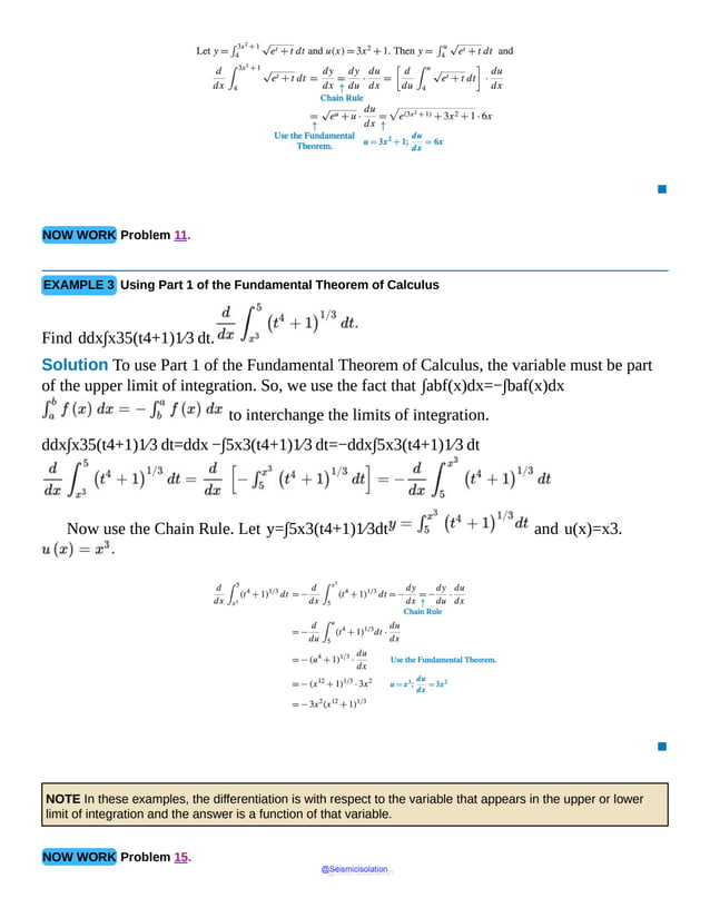
1028. 2 Use Part 2 of the Fundamental Theorem of Calculus
Part 1 of the Fundamental Theorem of Calculus establishes a relationship between the
derivative and the definite integral. Part 2 of the Fundamental Theorem of Calculus provides
a method for finding a definite integral without using Riemann sums.
THEOREM Fundamental Theorem of Calculus, Part 2
Let f be a function that is continuous on a closed interval [a,b]. If F is any
antiderivative of f on [a,b], then
∫abf(x)dx=F(b)−F(a)
IN WORDS If F′(x)= f(x), then ∫abf(x)dx= F(b)− F(a). That
is, if you can find an antiderivative of f, you can integrate f.
Proof Let I(x)=∫axf(t)dt. Then from Part 1 of the Fundamental Theorem
of Calculus, I= I(x) is continuous for a≤ x≤ b and differentiable for
a< x< b. So,
ddx∫axf(t)dt= f(x)a< x< b
That is, ∫axf(t)dt is an antiderivative of f. So, if F is any antiderivative of f,
then
F(x)=∫axf(t)dt+C
where C is some constant. Since F is continuous on [a,b], we have
F(a)=∫aaf(t)dt+CF(b)=∫abf(t)dt+C
Since, ∫aaf(t)dt=0, subtracting F(a) from F(b) gives
F(b)− F(a)=∫abf(t)dt
Since t is a dummy variable, we can replace t by x and the result follows.
▪
RECALL Any two antiderivatives of a function differ by a constant.
@Seismicisolation
@Seismicisolation

1029. NOTE For any constant C, [F(b)+C]-[F(a)+C]= F(b)- F(a).
In other words, it does not matter which antiderivative of f is chosen when using Part 2 of the Fundamental
Theorem of Calculus, since the same answer is obtained for every antiderivative.
As an aid in computation, we introduce the notation
∫abf(x)dx=F(x)ab=F(b)−F(a)
The notation F(x)ab also suggests that to find ∫abf(x)dx, we first find an
antiderivative F(x) of f(x). Then we write F(x)ab to represent F(b)
− F(a).
EXAMPLE 4 Using Part 2 of the Fundamental Theorem of Calculus
Use Part 2 of the Fundamental Theorem of Calculus to find:
a. ∫−21x2 dx
b. ∫0π⁄6cos x dx
c. ∫03⁄211−x2 dx
d. ∫121x dx
NOTE Table 6 in Section 4.8, page 344, provides a list of common antiderivatives.
Solution a. The function f(x)=x2 is continuous on the closed interval [−2,1].
An antiderivative of f is F(x)=x33. By Part 2 of the Fundamental
Theorem of Calculus,
∫−21x2dx=x33−21=133−−233=13+83=93=3
@Seismicisolation
@Seismicisolation

1030. b. The function f(x)=cos x is continuous on the closed interval 0,π6. An
antiderivative of f is F(x)=sin x. By Part 2 of the Fundamental Theorem of
Calculus,
∫0π⁄6cos x dx=sin x0π⁄6=sin π6−sin 0=12
c. The function f(x)=11−x2 is continuous on the closed interval 0,32.
An antiderivative of f is F(x)=sin−1x, provided | x|<1.
By Part 2 of the Fundamental Theorem of Calculus,
∫03⁄211−x2 dx=sin−1x03⁄2=sin−132−sin−10=π3−0=π3
d. The function f(x)=1x is continuous on the closed interval [1, 2]. An
antiderivative of f is F(x)=ln|x |. By Part 2 of the Fundamental Theorem of
Calculus,
∫121x dx=ln|x|12=ln 2−ln 1=ln 2−0=ln 2
▪
NOW WORK Problems 25 and 31.
EXAMPLE 5 Finding the Area Under a Graph
Find the area under the graph of f(x)=ex from −1 to 1.
Solution Figure 22 shows the graph of f(x)=ex on the closed interval [−1,1].
Since f is continuous on the closed interval [−1,1], the area A under the graph of f
from −1 to 1 is given by
A=∫−11ex dx=ex−11=e1−e−1= e−1e
@Seismicisolation
@Seismicisolation

1031. ▪
Figure 22 f(x)=ex,−1≤ x≤1
NOW WORK Problem 53.
3 Interpret the Integral of a Rate of Change
Part 2 of the Fundamental Theorem of Calculus states that, under certain conditions, if F is
an antiderivative of f, then
∫abf(x)dx= F(b)− F(a)
Since F is an antiderivative of f, then F′= f so
∫abF′(x)dx= F(b)− F(a)
In other words,
The integral from a to b of the rate of change of F equals the change
in F from a to b
That is,
∫abF′(x)dx=F(b)−F(a)
(4)
EXAMPLE 6 Interpreting an Integral Whose Integrand Is a Rate of Change
@Seismicisolation
@Seismicisolation

1032. The population of the United States is growing at the rate of P′(t)=2.867(1.009)t
million people per year, where t is the number of years since 2015.
a. Find ∫05P′(t)dt.
b. Interpret ∫05P′(t)dt in the context of the problem.
c. If the population of the United States was 320 million people in 2015, what is the
projected population in 2020?
Source: U.S. Census Bureau
Solution a. We use the Fundamental Theorem of Calculus, Part 2.
∫052.867(1.009)tdt=2.8671.009tln 1.00905An antiderivative
ofat is atlna.=2.8671.0095ln 1.009−1.0090ln 1.009=2.8671.0095−1ln 1.009≈14.661
b. Since P′(t) is the rate of change of the population P (in millions) with respect to
time t, in years,
∫05P′(t)dt= P(5)− P(0)
is the projected change in the population (in millions) of the United States from 2015 (t=0
) to 2020 (t=5 ). The population of the United States is projected to increase by
14.661 million people from 2015 to 2020.
c. The projected population of the United States in 2020 is
P(5)= P(0)+∫05P′(t)dt=320+14.661=334.661millionpeople
▪
NOW WORK Problem 63.
@Seismicisolation
@Seismicisolation

1033. Economists use calculus to identify the benefits and/or costs of an economic decision.
Marginal analysis is the process of identifying the benefits and/or costs of an economic
decision based on examining the incremental effect on total revenue and total cost caused by
a very small (just one unit) change in the output or input of each alternative.
Marginal profit P′(x) is the rate of change in profit that results from producing
and selling one more unit. Based on statement (4),
∫x1x2P′(t)dt= P(x2)− P(x1)= changeinprofitx1 to x2
EXAMPLE 7 Interpreting an Integral Whose Integrand Is Marginal Profit
The marginal profit P′ in dollars per unit for producing and selling x units of a product is
given by
P′(x)=x
Suppose 100 units have been produced and sold. Find the additional profit P from
producing and selling 21 more units.
Solution After 100 units have been sold, the profit from producing and selling 21 additional
units is given by
∫100121x dx=∫100121x1⁄2 dx=x3⁄232100121=2x3⁄23100121=23 (1213⁄2)−23 (1003⁄2)=23 (1331
The company earns $220.67 from selling an additional 21 units.
▪
The profit earned from producing and selling the first hundred units is ∫0100P
′(x)dx=23⋅1003⁄2=666.67, or $6.67 per unit. The
profit earned from producing and selling the additional 21 units is $220.67, or
$10.51 per additional unit. The profit margin is improving as sales increase.
NOW WORK Problem 65.
4 Interpret the Integral as an Accumulation Function
@Seismicisolation
@Seismicisolation

1034. If f is a function that is continuous and nonnegative on an interval [a,b], then the
definite integral ∫abf(x)dx exists and equals the area A under the graph of f
from a to b. See Figure 23(a).
Figure 23 (a) A=∫abf(x)dx
It
shows
a
shaded
area
under
the
curve
depicting
function
f
of
x
and
bounded
by
x
axis
and
the
vertical
Suppose we define the function F to be
F(x)=∫axf(t)dta≤x≤b
Since the independent variable x of F is the upper limit of integration of the definite
integral, we can interpret F as the area under the graph of f from a to the number x,
as shown in Figure 23(b). Notice that when x= a, then F(a)=∫aaf(t)dt=0
and when x= b, then F(b)=∫abf(t)dt= A.
Notice also that as x increases from a to b, the function F
also increases, accumulating more area as x goes from a to b. It is for this reason we
can describe F(x)=∫axf(t)dt as an accumulation function.
@Seismicisolation
@Seismicisolation

1035. Figure 23 (b) F(x)=∫axf(t)dt, a≤ x≤ b
A
perpendicular
from
the
point
x
which
lies
between
the
points
a
and
b
on
the
horizontal
axis
points
toward
the
curve.
It
shows
a
shaded
Now suppose f is not required to be nonnegative on the interval [a,b]. Then f
may be nonnegative on some subinterval(s) of [a,b] and negative on others. We examine
how this affects F(x)=∫axf(t)dt.
See Figure 24. On the interval [a,c1], the function f is nonnegative. As x
increases from a to c1, F(x)=∫axf(t)dt accumulates value and is
increasing. On the interval [c1,c2], f(t)≤0. As a result, the Riemann sums
∑i=1nf(ui)Δti for f on the interval [c1,c2] are negative.
Figure 24 F(x)=∫axf(t)dt
A
So as x increases from a to c2, the accumulation function F increases from a to
c1 and then starts to decrease as x goes from c1 to c2, possibly becoming negative.
@Seismicisolation
@Seismicisolation

1036. Then from c2 to b, the accumulation function F starts to increase again. The net
accumulation from a to b, given by ∫abf(t)dt, can be a positive number, a
negative number, or zero.
DEFINITION Accumulation Function
Let f be a function that is continuous on the closed interval [a,b]. The accumulation
function F associated with f over the interval [a,b] is defined as
F(x)=∫axf(t)dta≤ x≤ b
EXAMPLE 8 Interpreting an Integral as an Accumulation Function
The graph of f(t)=sint,0≤t≤2π is shown in Figure 25.
Figure 25 f(t)=sin t, 0≤ t≤2π
It
shows
a
shaded
area
under
the
curve
depicting
a. Find the accumulation function F associated with f over the interval [0,2π ].
b. Find F π2, F(π), F 3π2, and F(2π).
c. Interpret the results found in (b).
Solution a. The accumulation function F associated with f(t)=sin t over the
interval [0,2π] is
F(x)=∫0xsin tdt=−cos t0x=−cos x−(−cos 0)=−cos x+1
@Seismicisolation
@Seismicisolation

1037. b. Now use F(x)=−cos x+1 to determine F at the required numbers.
F π2=−cos π2+1=1F (π)=−cos π+1=1+1=2F 3π2=−cos 3π2+1=0+1=1F (2π)=−cos (2π)+1=
−1+1=0
c. The sine function is positive over the interval (0,π) and is negative over the interval
(π,2π). The accumulation function F of f(t)=sint increases from 0 to 1
to 2 as x increases from 0 to π and then will decrease from 2 to 1 to 0 as x
goes from π to 2π. The net accumulation over the interval [0,2π] equals 0.
▪
NOW WORK Problem 45.
5.3 Assess Your Understanding
Concepts and Vocabulary
1. According to Part 1 of the Fundamental Theorem of Calculus, if a function f is
continuous on a closed interval [a,b], then ddx∫axf(t)dt=________
for all numbers x in (a,b).
2. True or False By Part 2 of the Fundamental Theorem of Calculus, ∫abx dx= b− a.
3. True or False By Part 2 of the Fundamental Theorem of Calculus, ∫abf(x)dx= f(b)− f(a).
4. True or False ∫abF′(x)dx can be interpreted as the rate of change in F
from a to b.
Skill Building
In Problems 5–18, find each derivative using Part 1 of the Fundamental Theorem of
@Seismicisolation
@Seismicisolation

1038. Calculus.
5. ddx∫1xt2+1 dt
6. ddx∫3xt+1t dt
7. ddt∫0t(3+x2)3⁄2dx
8. ddx∫−4xt3+81⁄3dt
9. ddx∫1xln u du
10. ddt∫4texdx
11. ddx∫12x3t2+1 dt
12. ddx∫1xt4+5 dt
13. ddx∫2x5sec t dt
14. ddx∫31⁄xsin5t dt
15. ddx∫x5sin (t2)dt
16. ddx∫x3(t2−5)10 dt
17. ddx∫5x25(6t)2⁄3 dt
@Seismicisolation
@Seismicisolation

1039. 18. ddx∫x20e10t dt
In Problems 19–36, use Part 2 of the Fundamental Theorem of Calculus to find each definite
integral.
19. ∫−23dx
20. ∫−232 dx
21. ∫−12x3dx
22. ∫131x3 dx
23. ∫01u du
24. ∫18y3 dy
25. ∫π⁄6π⁄2csc2x dx
26. ∫0π⁄2cos x dx
27. ∫0π⁄4sec x tan xdx
28. ∫π⁄6π⁄2csc x cot x dx
29. ∫−10ex dx
30. ∫−10e−x dx
31. ∫1e1x dx @Seismicisolation
@Seismicisolation

1040. 32. ∫e11x dx
33. ∫0111+x2 dx
34. ∫02⁄211−x2 dx
35. ∫−18x2⁄3 dx
36. ∫04x3⁄2 dx
In Problems 37–42, find ∫abf(x)dx over the domain of f indicated in the graph.
37.
@Seismicisolation
@Seismicisolation

1041. 38.
39.
40.
@Seismicisolation
@Seismicisolation

1042. 41.
42.
In Problems 43–50,
a. Write the accumulation function F associated with f over the indicated interval as an
integral.
b. Find F at the given numbers.
c. Graph F.
43. f(t)=cos t, 0≤ t≤4π3 ; Fπ6, F π2 , F 4π3
44. f(t)=sin (2t) , 0≤ t≤3π2 ; F π6 , F π2 , F 3π2
@Seismicisolation
@Seismicisolation

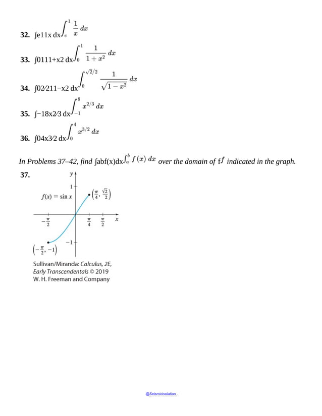
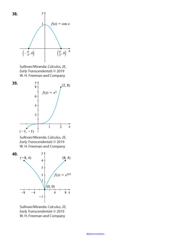
1043. 45. f(t)=t3 , −2≤ t≤3 ; F (−1) , F (0) , F (3)
46. f(t)=t3 , −8≤ t≤8 ; F (−1) , F (0) , F (8)
47. f(t)=4−t2, −1≤ t≤3 ; F(0),F(2),F(3)
48. f(t)=8−t3, 0≤ t≤4 ; F(1),F(2),F(4)
49. f(t)=t−2, 0≤ t≤9 ; F(1),F(4),F(9)
50. f(t)=t2−2t−3, 0≤ t≤5 ; F(1),F(3),F(5)
Applications and Extensions
51. Given that f(x)=(2x3−3)2 and f′(x)=12x2(2x3−3),
find ∫02[12x2(2x3−3)]dx.
52. Given that f(x)=(x2+5)3 and f′(x)=6x(x2+5)2,
find ∫−126x(x2+5)2 dx.
53. Area Find the area under the graph of f(x)=11−x2 from 0 to 12.
54. Area Find the area under the graph of f(x)=cosh x from −1 to 1.
55. Area Find the area under the graph of f(x)=1x2+1 from 0 to 3.
56. Area Find the area under the graph of f(x)=11+x2 from 0 to r, where
r>0. What happens as r→∞ ?
57. Area Find the area under the graph of y=1x from x=1 to x= r,
where r>1. Then examine the behavior of this area as r→∞.
58. Area Find the area under the graph of y=1x2 from x=1 to x= r,
where r>1. Then examine the behavior of this area as r→∞.
59. Interpreting an Integral The function R= R(t) models the rate of sales of a
corporation measured in millions of dollars per year as a function of the time t in years.
Interpret the integral ∫02R(t)dt=23 in the context of the problem.
60. Interpreting an Integral The function v= v(t) models the speed v in meters
@Seismicisolation
@Seismicisolation

1044. per second of an object at time t in seconds. Interpret the integral ∫010v(t)dt=4.8
in the context of the problem.
61. Interpreting an Integral Helium is leaking from a large advertising balloon at a rate of
H(t) cubic centimeters per minute, where t is measured in minutes.
a. Write an integral that models the change in the amount of helium in the balloon
over the interval a≤ t≤ b.
b. What are the units of the integral from (a)?
c. Interpret ∫0300H(t)dt=−100 in the context of the problem.
62. Interpreting an Integral Water is being added to a reservoir at a rate of w(t)
kiloliters per hour, where t is measured in hours.
a. Write an integral that models the change in the amount of water in the reservoir
over the interval a≤ t≤ b.
b. What are the units of the integral from (a)?
c. Interpret ∫036w(t)dt=100 in the context of the problem.
63. Population Growth The growth rate of a colony of bacteria is B′(t)=3.455(1.259)t
grams per hour, where t is the number of hours since time t=0.
a. Find ∫06B′(t)dt.
b. Interpret ∫06B′(t)dt in the context of the problem.
c. If 15 grams of bacteria are present at time t=0, how many grams of bacteria
are present after 6 h?
64. Return on Investment An investment in a hedge fund is growing at a continuous rate
of A′(t)=1105.17(1.105)t dollars per year.
a. Find ∫010A′(t)dt.
b. Interpret ∫010A′(t)dt in the context of the problem.
c. If initially $1000 is invested, what is the value of the investment after 10 years.
65. Increase in Revenue The marginal revenue function R′(x) for selling x units of
a product is R′(x)=x3 (in hundreds of dollars per unit).
@Seismicisolation
@Seismicisolation

1045. a. Interpret ∫abR′(x)dx in the context of the problem.
b. How much additional revenue is attained if sales increase from 40 to 50 units?
66. Increase in Cost The marginal cost function C′(x) of producing x thousand
units of a product is C′(x)=2x+6 thousand dollars.
a. Interpret ∫abC′(x)dx in the context of the problem.
b. What does it cost the company to increase production from 10,000 units to 13,000
units?
67. Free Fall The speed v of an object dropped from rest is given by v(t)=9.8t,
where v is in meters per second and time t is in seconds.
a. Express the distance traveled in the first 5.2 s as an integral.
b. Find the distance traveled in 5.2 s.
68. Area Find h so that the area under the graph of y2=x3,0≤ x≤4,y≥0,
is equal to the area of a rectangle of base 4 and height h.
69. Area If P is a polynomial that is positive for x>0, and for each k>0 the
area under the graph of P from x=0 to x= k is k3+3k2+6k,
find P.
70. Put It Together If f(x)=∫0x1t3+2 dt, which of the following is
false?
a. f is continuous at x for all x≥0
b. f(1)>0
c. f(0)=12
d. f′(1)=13
In Problems 71–74:
a. Use Part of 2 the Fundamental Theorem of Calculus to find each definite integral.
b. Determine whether the integrand is an even function, an odd function, or neither.
c. Can you make a conjecture about the definite integrals in (a) based on the analysis from
(b)? @Seismicisolation
@Seismicisolation

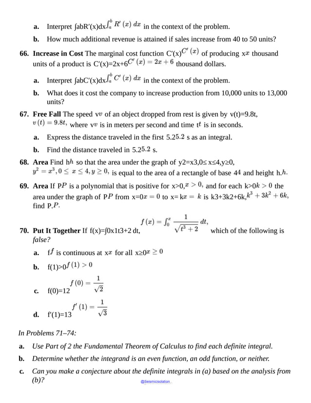
1046. 71. ∫04x2dx and ∫−44x2dx
72. ∫04x3dx and ∫−44x3dx
73. ∫0π⁄4sec2x dx and ∫−π⁄4π⁄4sec2 x dx
74. ∫0π⁄4sin x dx and ∫−π⁄4π⁄4sin x dx
75. Area Find c, 0< c<1, so that the area under the graph of y=x2 from
0 to c equals the area under the same graph from c to 1.
76. Area Let A be the area under the graph of y=1x from x= m to x=2m,
m>0. Which of the following is true about the area A ?
a. A is independent of m.
b. A increases as m increases.
c. A decreases as m increases.
d. A decreases as m increases when m<12 and increases as m increases
when m>12.
e. A increases as m increases when m<12 and decreases as m increases
when m>12.
77. Put It Together If F is a function whose derivative is continuous for all real x, find
limh→0 1h∫cc+hF′(x)dx
78. Suppose the closed interval 0,π2 is partitioned into n subintervals, each of
length Δx, and ui is an arbitrary number in the subinterval [xi−1,xi],
i=1,2,…, n. Explain why
limn→∞∑i=1n(cos ui) Δx=1
@Seismicisolation
@Seismicisolation

1047. 79. The interval [0,4] is partitioned into n subintervals, each of length Δx , and a
number ui is chosen in the subinterval [xi−1,xi], i=1,2,…, n.
Find limn→∞∑i=1n(eui Δx)
80. If u and ν are differentiable functions and f is a continuous function, find a formula
for
ddx ∫u(x)ν(x)f(t)dt
81. Suppose that the graph of y= f(x) contains the points (0,1) and (2,5).
Find ∫02f′(x)dx. (Assume that f′ is continuous.)
82. If f′ is continuous on the interval [a,b], show that
∫abf(x)f′(x)dx=12[f(b)]2−[f(a)]2
Hint: Look at the derivative of F(x)=f(x)22.
83. If f′′ is continuous on the interval [a,b], show that
∫abxf′′(x)dx= bf′(b)− af′(a)− f(b)+f(a)
Hint: Look at the derivative of F(x)= xf′(x)− f(x).
Challenge Problems
84. What conditions on f and f′ guarantee that f(x)=∫0xf′(t)dt ?
85. Suppose that F is an antiderivative of f on the interval [a,b]. Partition [a,b]
into n subintervals, each of length Δxi=xi−xi−1, i=1,2,…,n.
a. Apply the Mean Value Theorem for derivatives to F in each subinterval [xi−1,xi]
to show that there is a number ui in the subinterval for which F(xi)
− F(xi−1)= f(ui)Δxi.
b. Show that ∑i=1n[F(xi)− F(xi−1)]= F(b)− F(a).
@Seismicisolation
@Seismicisolation

1048. c. Use parts (a) and (b) to explain why
∫abf(x)dx= F(b)− F(a).
(In this alternate proof of Part 2 of the Fundamental Theorem of Calculus, the
continuity of f is not assumed.)
86. Given y=x2−1(4− x), 1≤ x≤ a, for what number a
will ∫1ay dx have a maximum value?
87. Find a>0, so that the area under the graph of y= x+1x from a to
(a+1) is minimum.
88. If n is a known positive integer, for what number c is
∫1cxn−1 dx=1n
89. Let f(x)=∫0xdt1−t2,0< x<1.
a. Find ddx f(sin x).
b. Is f one-to-one?
c. Does f have an inverse?
1. = NOW WORK problem
= Graphing technology recommended
= Computer Algebra System recommended
@Seismicisolation
@Seismicisolation

1049. (1)
5.4 Properties of the Definite Integral
OBJECTIVES When you finish this section, you should be able to:
1 Use properties of the definite integral
2 Work with the Mean Value Theorem for Integrals
3 Find the average value of a function
4 Interpret integrals involving rectilinear motion
We have seen that there are properties of limits that make it easier to find limits, properties of
continuity that make it easier to determine continuity, and properties of derivatives that make
it easier to find derivatives. Here we investigate several properties of the definite integral that
will make it easier to find integrals.
1 Use Properties of the Definite Integral
Properties (1) through (4) in this section require that a function be integrable.
Remember, in Section 5.2 we stated two theorems that guarantee a function f is
integrable.
A function f that is continuous on a closed interval [a,b] is integrable over [a,b].
A function f that is bounded on a closed interval [a,b] and has at most a finite
number of discontinuities on [a,b] is integrable over [a,b].
Proofs of most of the properties in this section require the use of the definition of the
definite integral. However, if the condition is added that the integrand has an antiderivative,
then the Fundamental Theorem of Calculus can be used to establish the properties. We will
use this added condition in the proofs included here.
NOTE From now on, we will refer to Parts 1 and 2 of the Fundamental Theorem of Calculus simply as the
Fundamental Theorem of Calculus.
THEOREM The Integral of the Sum of Two Functions
If two functions f and g are integrable on the closed interval [a,b], then
∫ab[f(x)+g(x)]dx=∫abf(x)dx+∫abg(x)dx
@Seismicisolation
@Seismicisolation

1050. (2)
IN WORDS The integral of a sum equals the sum of the integrals.
Proof For the proof, we assume that the functions f and g are continuous on [a,b]
and that F and G are antiderivatives of f and g, respectively, on (a,b). Then F
′=f and G′=g on (a,b).
Also, since (F+G)′=F′+G′=f+g, then F+G is an
antiderivative of f+g on (a,b). Now
∫ab[f(x)+g(x)]dx=F(x)+G(x)ab=[F(b)+G(b)]−[F(a)+G(a)]=[F(b)−F(a)]+[G(b)
−G(a)]=∫abf(x)dx+∫abg(x) dx
▪
EXAMPLE 1 Using Property (1) of the Definite Integral
∫01(x2+ex)dx=∫01x2dx+∫01ex dx=x3301+ex01=133−0+e1−e0=13+e−1=e−23
▪
NOW WORK Problem 17.
THEOREM The Integral of a Constant Times a Function
If a function f is integrable on the closed interval [a,b] and k is a constant, then
∫abkf (x)dx=k∫abf (x)dx
IN WORDS A constant factor can be factored out of an integral.
@Seismicisolation
@Seismicisolation

1051. You are asked to prove this theorem in Problem 105 if f is continuous on the interval
[a,b] and f has an antiderivative on the interval (a,b).
EXAMPLE 2 Using Property (2) of the Definite Integral
▪
NOW WORK Problem 19.
Properties (1) and (2) can be extended as follows:
THEOREM
Suppose each of the functions f1, f2,…,fn is integrable on the closed interval
[a,b]. If k1, k2, …, kn are constants, then
∫ab k1f1(x)+k2f2(x)+⋯+knfn(x)dx=k1∫abf1(x)dx+k2∫abf2(x)dx+⋯+kn∫abfn(x)dx
You are asked to prove this theorem in Problem 106 if each function is continuous on the
interval [a,b] and each function has an antiderivative on the interval (a,b).
EXAMPLE 3 Using Property (3) of the Definite Integral
Find ∫123x3−6x2−5x+42x dx.
Solution The function f(x)=3x3−6x2−5x+42x is continuous
on the closed interval [1,2] so it is integrable on [1,2]. Using algebra and
properties of the definite integral,
∫123x3−6x2−5x+42x dx=∫12 32 x2−3x−52+2xdx=32∫12x2dx−3∫12xdx
−52∫12dx+2∫121xdxUse property (3).=32x3312−3x2212−52x12+2ln|x|12Use the
Fundamental Theorem of Calculus.=12 (8−1)−32 (4−1)−52 (2−1)+2(ln 2−ln 1)=−72+2 ln 2
@Seismicisolation
@Seismicisolation

1052. (4)
▪
NOW WORK Problem 29.
The next property states that a definite integral of a function f from a to b can be
evaluated in pieces.
THEOREM
If a function f is integrable on an interval containing the numbers a, b, and c, then
∫abf(x)dx=∫acf(x)dx+∫cbf (x)dx
A proof of this theorem for a function f that is continuous on [a,b ] is given in
Appendix B. A proof for the more general case can be found in most advanced calculus
books.
In particular, if f is continuous and nonnegative on a closed interval [a,b] and if c
is a number between a and b, then property (4) has a simple geometric interpretation, as
seen in Figure 26.
@Seismicisolation
@Seismicisolation

1053. Figure 26
The
area
under
the
curve
is
divided
into
two
partitions
A
sub(1)
and
A
sub(2)
with
vertical
lines
drawn
from
x
equal
to
EXAMPLE 4 Using Property (4) of the Definite Integral
a. If f is integrable on the closed interval [2,7], then
∫27f (x)dx=∫24f (x)dx+∫47f (x)dx
b. If g is integrable on the closed interval [3,25], then
∫310g (x)dx=∫325g (x)dx+∫2510g (x)dx
▪
Example 4(b) illustrates that the number c need not lie between a and b.
NOW WORK Problem 47.
Property (4) is useful when integrating piecewise-defined functions.
EXAMPLE 5 Using Property (4) to Find the Area Under the Graph of a Piecewise-defined Function
Find the area A under the graph of
@Seismicisolation
@Seismicisolation

1054. f (x)=x2if0≤x<10100if10≤x≤15
from 0 to 15.
Solution See Figure 27. Since f is continuous and nonnegative on the closed interval
[0,15], then ∫015f(x)dx exists and equals the area A under the graph of
f from 0 to 15. We break the integral at x=10, where the rule for the function
changes.
∫015f (x)dx=∫010f (x)dx+∫1015f (x)dx=∫010x2 dx+∫1015100dx=x33010+100x1015=10003+500
The area under the graph of f is approximately 833.333 square units.
▪
Figure 27 A=∫015f (x)dx
The
curve
increases
NOW WORK Problem 39.
The next property establishes bounds on a definite integral.
@Seismicisolation
@Seismicisolation

1055. (5)
THEOREM Bounds on an Integral
If a function f is continuous on a closed interval [a,b] and if m and M denote
the absolute minimum value and the absolute maximum value, respectively, of f on [a,b],
then
m(b−a)≤∫abf (x)dx≤M(b−a)
A proof of this theorem is given in Appendix B.
If f is nonnegative on [a,b], then the inequalities in (5) have a geometric
interpretation. In Figure 28, the area of the shaded region is ∫abf (x)dx. The
rectangle of width b−a and height m has area m(b−a). The rectangle of
width b−a and height M has area M(b−a). The areas of the three regions
are numerically related by the inequalities in the theorem.
Figure 28
It
shows
a
shaded
area
under
the
EXAMPLE 6 Using Property (5) of Definite Integrals
a. Find an upper bound and a lower bound for the area A under the graph of f (x)=sinx
from 0 to π.
b. Find the actual area under the graph.
Solution The graph of f is shown in Figure 29. Since f (x)≥0 for all x in the
@Seismicisolation
@Seismicisolation

1056. closed interval [0,π], the area A under its graph is given by the definite integral,
∫0πsin xdx.
Figure 29 f (x)=sin x,0≤x≤π
a. From the Extreme Value Theorem, f has an absolute minimum value and an absolute
maximum value on the interval [0, π]. The absolute maximum of f occurs at x=π2,
and its value is f π2=sin π2=1. The absolute minimum occurs at
x=0 and at x=π ; the absolute minimum value is f (0)=sin 0=0=f (π).
Using the inequalities in (5), the area under the graph of f is
bounded as follows:
0≤∫0πsin xdx≤π
NEED TO REVIEW? The Extreme Value Theorem is discussed in Section 4.2, p. 274.
b. The actual area under the graph is
A=∫0πsin xdx=−cos x0π=−cos π+cos 0=1+1=2 square units
▪
NOW WORK Problem 57.
2 Work with the Mean Value Theorem for Integrals
@Seismicisolation
@Seismicisolation

1057. (6)
Suppose f is a function that is continuous and nonnegative on a closed interval [a,b].
Figure 30 suggests that the area under the graph of f from a to b, ∫abf (x)dx,
is equal to the area of some rectangle of width b−a and height f (u) for some
choice (or choices) of u in the interval [a,b].
Figure 30 ∫abf (x)dx=f (u)(b−a)
It
shows
a
shaded
area
of
a
rectangle
with
width
b
minus
a
and
height
f
of
u.
In more general terms, for every function f that is continuous on a closed interval [a,b],
there is some number u (not necessarily unique) in the interval [a,b] for which
∫abf (x)dx=f (u)(b−a)
This result is known as the Mean Value Theorem for Integrals.
THEOREM Mean Value Theorem for Integrals
If a function f is continuous on a closed interval [a,b], there is a real number u,
a≤u≤b, for which
∫abf (x)dx=f (u)(b−a)
Proof Let f be a function that is continuous on a closed interval [a,b].
If f is a constant function, say, f (x)=k, on [a,b], then
∫abf (x)dx=∫abkdx=k(b−a)=f (u)(b−a)
@Seismicisolation
@Seismicisolation

1058. for any choice of u in [a,b].
If f is not a constant function on [a,b], then by the Extreme Value Theorem, f
has an absolute maximum and an absolute minimum on [a,b]. Suppose f assumes its
absolute minimum at the number c so that f (c)=m ; and suppose f assumes its
absolute maximum at the number C so that f (C)=M. Then by the Bounds on an
Integral Theorem (5), we have
m(b−a)≤∫abf (x)dx≤M(b−a)for all x in [a,b]
Divide each part by (b−a) and replace m by f (c) and M by f (C).
Then
f (c)≤1b−a∫abf (x)dx≤f (C)
Since 1b−a∫abf (x)dx is a real number between f (c) and f (C), it
follows from the Intermediate Value Theorem that there is a real number u between c and
C, for which
f (u)=1b−a∫abf (x)dx
That is, there is a real number u, a≤u≤b, for which
∫abf (x)dx=f (u)(b−a)
▪
NEED TO REVIEW? The Intermediate Value Theorem is discussed in Section 1.3, pp. 109–110.
EXAMPLE 7 Using the Mean Value Theorem for Integrals
Find the number(s) u guaranteed by the Mean Value Theorem for Integrals for ∫26x2dx.
Solution Since the function f (x)=x2 is continuous on the closed interval [2, 6],
the Mean Value Theorem for Integrals guarantees there is a number u, 2≤u≤6,
for which
@Seismicisolation
@Seismicisolation

1059. ∫26x2dx=f (u)(6−2)=4u2f (u)=u2
Integrating, we have
∫26x2dx=x3326=13 (216−8)=2083
Then
2083=4u2u2=5232≤u≤6u=523≈4.163Disregard the negative solution since u>0.
▪
NOW WORK Problem 59.
3 Find the Average Value of a Function
We know from the Mean Value Theorem for Integrals that if a function f is continuous on a
closed interval [a,b], there is a real number u, a≤u≤b, for which
∫abf (x)dx=f (u)(b−a)
This means that if the function f is also nonnegative on the closed interval [a,b],
the area enclosed by a rectangle of height f (u) and width b−a equals the area
under the graph of f from a to b. See Figure 31. Consequently, f (u) can be thought
of as an average value, or mean value, of f over [a,b].
@Seismicisolation
@Seismicisolation

1060. (7)
Figure 31 ∫abf (x)dx=f (u)(b−a)
It
shows
a
shaded
area
of
a
rectangle
with
width
b
minus
a
and
height
f
of
u.
We can obtain the average value of f over [a,b] for any function f that is
continuous on the closed interval [a,b] by partitioning [a,b] into n subintervals
[a,x1],[x1,x2],…,[xi−1,xi],…,[xn−1,b]
each of length Δx=b−an, and choosing a number ui in each of the n
subintervals. Then an approximation of the average value of f over the interval [a,b]
is
f (u1)+f (u2)+⋯+f (un)n
Now multiply (7) by b−ab−a to obtain
f (u1)+f (u2)+⋯+f (un)n=1b−a f (u1)b−an+f (u2)b−an+⋯+f (un)b−an=1b
−a[f (u1)Δx+f (u2)Δx+⋯+f (un)Δx]=1b−a∑i=1nf(ui) Δ x
@Seismicisolation
@Seismicisolation

1061. (8)
This sum approximates the average value of f. As the length of each subinterval gets
smaller, the sums become better approximations to the average value of f on [a,b].
Furthermore, ∑i = 1nf (ui) Δ x are Riemann sums, so limx→∞ ∑i = 1nf(ui) Δ x
is a definite integral. This suggests the following definition:
DEFINITION Average Value of a Function over an Interval
Let f be a function that is continuous on the closed interval [a,b]. The average
value ȳ of f over [a,b] is
ȳ=1b−a∫abf (x)dx
IN WORDS The average value ȳ of a function f equals the value f (u) in the Mean Value Theorem for
Integrals.
EXAMPLE 8 Finding the Average Value of a Function
Find the average value of f (x)=x3 on the closed interval [0,2].
Solution The average value of f (x)=x3 on the closed interval [0,2] is given
by
ȳ=1b−a∫abf (x)dx=12−0∫02x3dx=12x4402=12 164=2
@Seismicisolation
@Seismicisolation

1062. The average value of f on [0,2] is ȳ=2.
▪
The function f and its average value are graphed in Figure 32.
Figure 32 f (x)=x3,0≤x≤2
NOW WORK Problem 65.
4 Interpret Integrals Involving Rectilinear Motion
For an object in rectilinear motion moving with velocity v,
The net displacement of an object whose motion begins at t=a and ends at t=b
is given by
∫abv(t)dt
The total distance traveled by the object from t=a to t=b is given by
∫ab|v(t)|dt
If v(t)≥0, for a≤t≤b, then the net displacement and the total
distance traveled are equal.
Remember speed and velocity are not the same thing. Speed measures how fast an object
is moving regardless of direction. Velocity measures both the speed and the direction of an
@Seismicisolation
@Seismicisolation

1063. object. Because of this, velocity can be positive, negative, or zero. Speed is the absolute
value of velocity. So ∫abv(t)dt is a sum of signed distances and ∫ab|v(t)|dt
is a sum of actual distances traveled.
EXAMPLE 9 Interpreting an Integral Involving Rectilinear Motion
An object in rectilinear motion is moving along a horizontal line with velocity
v(t)=3t2−18t+15 (in meters per minute) for time 0≤t≤6
min.
a. Find the net displacement of the object from t=0 to t=6. Interpret the result
in the context of the problem.
b. Find the total distance traveled by the object from t=0 to t=6 and interpret the
result.
Solution a. The net displacement of the object from t=0 to t=6 is given by
∫06v(t)dt=∫06(3t2−18t+15)dt=t3−9t2+15t06=63−9⋅62+15⋅6−0=−18
After moving from t=0 to t=6, the object is 18 m to the left of where it was at
t=0.
b. The total distance traveled by the object from t=0 to t=6 min is given by
∫06|v(t)|dt.
Since v(t)=3t2−18t+15=3(t−1)(t−5)
we find that v(t)≥0 if 0≤t≤1 or if 5≤t≤6 and v(t)≤0
if 1≤t≤5. Now express |v(t)| as the piecewise-defined function
|v(t)|=v(t)=3t2−18t+15if0≤t≤1−v(t)=−(3t2−18t+15)if1<t<5v(t)=3t2−18t+15if5≤t≤6
Then
∫06|v(t)|dt=∫01v(t)dt+∫15[−v(t)]dt+∫56v(t)dt=[t3−9t2+15t]01−[t3−9t2+15t]15+
[t3−9t2+15t]56=(7−0)−(−25−7)+[−18−(−25)]=7+32+7=46
@Seismicisolation
@Seismicisolation

1064. The object traveled a total distance of 46 m from t=0 to t=6 min.
▪
Figure 33 shows the distinction between the net displacement and the total distance
traveled by the object assuming that the object is at the origin when the motion starts.
Figure 33
NOW WORK Problem 79.
5.4 Assess Your Understanding
Concepts and Vocabulary
1. True or False ∫23(x2+x)dx=∫23x2dx+∫23xdx
2. True or False ∫035ex2dx=∫035dx⋅∫03ex2dx
3. True or False
∫05(x3+1)dx=∫0−3(x3+1)dx+∫−35(x3+1)dx
4. If f is continuous on an interval containing the numbers a, b, and c, and if
∫ac f (x)dx=3 and ∫cb f (x)dx=−5, then ∫ab f (x)dx=
@Seismicisolation
@Seismicisolation

1065. ____________.
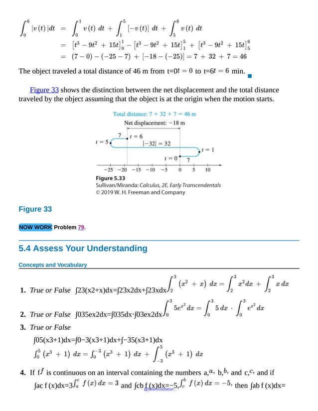
5. If a function f is continuous on the closed interval [a,b], then ȳ=1b−a∫abf (x)dx
is the ________ of f over [a, b].
6. True or False If a function f is continuous on a closed interval [a, b] and if m
and M denote the absolute minimum value and the absolute maximum value,
respectively, of f on [a, b], then
m≤∫abf (x)dx≤M
Skill Building
In Problems 7–16, find each definite integral given that ∫13f (x)dx=5,
∫13g(x)dx=−2, ∫35f (x)dx=2, ∫35g(x)dx=1.
7. ∫13[f (x)−g(x)]dx
8. ∫13[f (x)+g(x)]dx
9. ∫13[5f (x)−3g(x)]dx
10. ∫13[3f (x)+4g(x)]dx
11. ∫15[2f (x)−3g(x)]dx
12. ∫15[f (x)−g(x)]dx
13. ∫13[5f (x)−3g(x)+7]dx
14. ∫13[f (x)+4g(x)+2x]dx
15. ∫15[2f (x)−g(x)+3x2]dx @Seismicisolation
@Seismicisolation

1066. 16. ∫15[5f (x)−3g(x) −4]dx
In Problems 17–36, find each definite integral using the Fundamental Theorem of Calculus
and properties of the definite integral.
17. ∫01(t2−t3⁄2)dt
18. ∫−20(x+x2)dx
19. ∫π⁄2π4 sin xdx
20. ∫0π⁄23 cos xdx
21. ∫−π⁄4π⁄4(1+2sec xtan x)dx
22. ∫0π⁄4(1+sec2 x)dx
23. ∫14(x−4x)dx
24. ∫01(t25+1)dt
25. ∫−23[(x−1)(x+3)]dx
26. ∫01(z2+1)2dz
27. ∫12x2−12x4dx
28. ∫1e5s2+ss2 ds
29. ∫01e2x−1exdx
@Seismicisolation
@Seismicisolation

1067. 30. ∫01e2x+4e−xdx
31. ∫π⁄3π⁄2x sin x+2xdx
32. ∫π⁄6π⁄2x cos x−4xdx
33. ∫12x2 sinh x+2x2dx
34. ∫14x cosh x−xxdx
35. ∫01⁄2 5+11−x2dx
36. ∫01 1+51+x2dx
In Problems 37–42, use properties of integrals and the Fundamental Theorem of Calculus to
find each integral.
37. ∫−21f (x)dx, where f (x)=1ifx<0x2+1ifx≥0
38. ∫−12f (x)dx, where f (x)=x+1ifx<0x2+1ifx≥0
39. ∫−22f (x)dx, where f (x)=3xif−2≤x<02x2if0≤x≤2
40. ∫04h(x)dx, where h(x)=x−2if0≤x≤22−xif2<x≤4
@Seismicisolation
@Seismicisolation

1068. 41. ∫−π⁄2π⁄2f (x)dx, where f (x)=x2+xif−π2≤x≤0sin xif0<x<π422ifπ4≤x≤π2
42. ∫05f (x)dx, where f (x)=x3−8x−2if0≤x<14x+3if1≤x≤5
In Problems 43–46, the domain of f is a closed interval [a,b] . Find ∫ab f (x)dx
.
43.
@Seismicisolation
@Seismicisolation

1069. 44.
45.
@Seismicisolation
@Seismicisolation

1070. 46.
In Problems 47–50, use properties of definite integrals to verify each statement. Assume that
all integrals involved exist.
47. ∫311 f (x) dx − ∫711 f (x) dx = ∫37 f (x) dx
48. ∫−26 f (x) dx−∫36f (x) dx=∫−23 f (x) dx
49. ∫04f (x) dx−∫46f (x) dx=∫06f (x) dx
50. ∫−13f (x) dx−∫53f (x) dx=∫−15f (x) dx
In Problems 51–58, use the Bounds on an Integral Theorem to obtain a lower estimate and
an upper estimate for each integral.
51. ∫13(5x+1)dx
52. ∫01(1−x)dx
53. ∫π⁄4π⁄2sin xdx
@Seismicisolation
@Seismicisolation

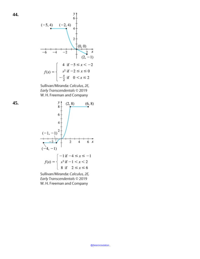
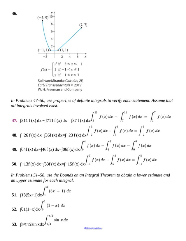
1071. 54. ∫π⁄6π⁄3cos xdx
55. ∫011+x2dx
56. ∫−111+x4dx
57. ∫01exdx
58. ∫1101x dx
In Problems 59–64, for each integral find the number(s) u guaranteed by the Mean Value
Theorem for Integrals.
59. ∫03(2x2+1)dx
60. ∫02(2−x3)dx
61. ∫04x2dx
62. ∫04(−x)dx
63. ∫02πcos xdx
64. ∫−π⁄4π⁄4 sec x tan xdx
In Problems 65–74, find the average value of each function f over the given interval.
65. f (x)=ex over [0,1]
66. f (x)=1x over [1,e]
67. f (x)=x2⁄3 over [−1,1]
@Seismicisolation
@Seismicisolation

1072. 68. f (x)=x over [0,4]
69. f (x)=sin x over 0,π2
70. f (x)=cos x over 0,π2
71. f (x)=1−x2 over [−1,1]
72. f (x)=16−x2 over [−4,4]
73. f (x)=ex − sin x over 0, π2
74. f (x)=x+ cos x over 0, π2
In Problems 75–78, find:
a. The area under the graph of the function over the indicated interval.
b. The average value of each function over the indicated interval.
c. Interpret the results geometrically.
75. [−1,2]
76. [−2,1]
@Seismicisolation
@Seismicisolation

1073. 77. [−1,2]
78. 0, 3π4
In Problems 79–82, an object in rectilinear motion is moving along a horizontal line with
velocity v over the indicated interval.
a. Find the net displacement of the object. Interpret the result in the context of the
problem.
@Seismicisolation
@Seismicisolation

1074. b. Find the total distance traveled by the object and interpret the result.
79. v(t)=6t2+12t−18 m⁄min;0≤t≤3
80. v(t)=t2−2t−8 m⁄min;0≤t≤6
81. v(t)=t3+2t2−8t m⁄s;−2≤t≤3
82. v(t)=t3+5t2−6t m⁄s;−1≤t≤3
Applications and Extensions
In Problems 83–86, find the indicated derivative.
83. ddx∫x4xt2+4dt
84. ddx∫xx2(t2+4)3⁄2dt
85. ddx∫x2x3ln tdt
86. ddx∫−xx2et2dt
In Problems 87–90, find each definite integral using the Fundamental Theorem of Calculus
and properties of definite integrals.
87. ∫−23(x+|x |)dx
88. ∫03|x−1|dx
89. ∫02|3x−1|dx
90. ∫05|2−x|dx
91. Average Temperature A rod 3 m long is heated to 25x∘C, where x is the
distance in meters from one end of the rod. Find the average temperature of the rod.
92. Average Daily Rainfall The rainfall per day, x days after the beginning of the year, is
@Seismicisolation
@Seismicisolation

1075. modeled by the function r(x)=0.00002(6511+366x−x2),
measured in centimeters. Find the average daily
rainfall for the first 180 days of the year.
93. Structural Engineering A structural engineer designing a member of a structure must
consider the forces that will act on that member. Most often, natural forces like snow,
wind, or rain distribute force over the entire member. For practical purposes, however,
an engineer determines the distributed force as a single resultant force acting at one
point on the member. If the distributed force is given by the function W=W(x),
in newtons per meter (N⁄M) , then the magnitude FR of the
resultant force is
FR=∫abW(x)dx
The position x of the resultant force measured in meters from the origin is given
by
x−=∫ab x W(x)dx∫abW(x)dx
If the distributed force is W(x)=0.75x3, 0≤x≤5, find:
a. The magnitude of the resultant force.
b. The position from the origin of the resultant force.
Source: Problem contributed by the students at Trine University, Avalon, IN.
94. Chemistry: Enthalpy In chemistry, enthalpy is a measure of the total energy of a
system. For a nonreactive process with no phase change, the change in enthalpy ΔH
is given by ΔH= ∫T1T2CpdT, where Cp is the specific heat of the
system in question. The specific heat per mol of the chemical benzene is
Cp=0.126+(2.34×10−6)T,
where Cp is in kJ⁄ mol∘C, and T is in degrees Celsius.
a. What are the units of the change in enthalpy ΔH?
b. What is the change in enthalpy ΔH associated with increasing the temperature of 1.0 mol of benzene from
20∘C to 40∘C ?
c. What is the change in enthalpy ΔH associated with increasing the temperature of 1.0 mol of benzene from
20∘C to 60∘C ?
d. Does the enthalpy of benzene increase, decrease, or remain constant as the temperature increases?
@Seismicisolation
@Seismicisolation

1076. Source: Problem contributed by the students at Trine University, Avalon, IN.
95. Average Mass Density The mass density of a metal bar of length 3 m is given by
ρ(x)=1000+x−x kilograms per cubic meter, where x is the
distance in meters from one end of the bar. What is the average mass density over the
length of the entire bar?
96. Average Velocity The velocity at time t, in m⁄s , of an object in rectilinear motion
is given by v(t)=4π cos t. What is the average velocity of the object over
the interval 0≤t≤π ?
97. Average Area What is the average area ofall circles whose radii are between 1 and 3 m?
98. Area
a. Use properties of integrals and the Fundamental Theorem of Calculus to find the area under the graph of y=3−|x|
from −3 to 3.
b. Check your answer by using elementary geometry.
99. Area
a. Use properties of integrals and the Fundamental Theorem of Calculus to find the area under the graph of y=1−12 x
from −2 to 2.
b. Check your answer by using elementary geometry. See the figure.
The
curve
of
function
f
of
x
is
a
100. Area Let A be the area in the first quadrant that is enclosed by the graphs of y=3x2,
y=3x, the x -axis, and the line x=k, where k>1, as
shown in the figure.
a. Find the area A as a function of k.
b. When the area is 7, what is k ?
c. If the area A is increasing at the constant rate of 5 square units per second, at what rate is k increasing when
k=15 ?
@Seismicisolation
@Seismicisolation

1077. It
shows
shaded
area
between
the
curves
for
y
equal
3x
square,
y
equals
3
by
x
and
a
vertical
line
x
equals
k.
101. Rectilinear Motion A car starting from rest accelerates at the rate of 3 m⁄s2.
Find its average speed over the first 8 s.
102. Rectilinear Motion A car moving at a constant speed of 80 miles per hour begins to
decelerate at the rate of 10 mi/h2. Find its average speed over the next 10 min.
103. Average Slope
a. Use the definition of average value of a function to find the average slope of the graph of y=f (x),
where a≤x≤b. (Assume that f′ is continuous.)
b. Give a geometric interpretation.
104. What theorem guarantees that the average slope found in Problem 103 is equal to f′(u)
for some u in [a,b]? What different theorem guarantees the same thing?
(Do you see the connection between these theorems?)
105. Prove that if a function f is continuous on a closed interval [a,b] and if k is a
constant, then ∫abkf (x)dx=k∫abf (x)dx. Assume f has an
antiderivative.
106. Prove that if the functions f1, f2,…,fn are continuous on a closed interval
[a,b] and if k1, k2,…,kn are constants, then
∫ab[k1 f1(x)+k2 f2(x)+⋯+kn fn(x)]dx=k1∫abf1(x)dx+k2∫abf2(x)dx+⋯+kn∫abfn(x)dx
Assume each function f has an antiderivative.
@Seismicisolation
@Seismicisolation

1078. 107. Area The area under the graph of y =cos x from −π2 to π2 is
separated into two parts by the line x=k, −π2<k<π2, as shown in
the figure. If the area under the graph of y from −π2 to k is three times the area
under the graph of y from k to π2, find k.
It
shows
shaded
area
between
the
curve
for
y
equals
sin
x
and
vertical
line
x
equals
k.
108. Displacement of a Damped Spring The net displacement x in meters of a damped
spring from its equilibrium position at time t seconds is given by
x(t)=1510 e−t sin 15t+32 e−t cos 15t
a. What is the net displacement of the spring at t=0?
b. Graph the displacement for the first 2 s of the spring’s motion.
c. Find the average displacement of the spring for the first 2 s of its motion.
109. Area Let
f (x)=|x4+3.44x3 − 0.5041x2 − 5.0882x+1.1523|
be defined on the interval [−3,1]. Find the area under the graph of f.
110. If f is continuous on [a,b], show that the functions defined by
f (x)=∫cxf (t)dtG(x)=∫dxf (t)dt
for any choice of c and d in (a,b) always differ by a constant. Also show that
f (x)−G(x)=∫cdf (t)dt
@Seismicisolation
@Seismicisolation

1079. 111. Put It Together Suppose a<c<b and the function f is continuous on [a,b]
and differentiable on (a,b). Which of the following is not necessarily true?
I. ∫abf (x)dx=∫acf (x)dx+∫cbf (x)dx.
II. There is a number d in (a,b) for which
f′(d)=f (b)−f (a)b−a
III. ∫abf (x)dx≥0.
IV. limx→c f (x) = f (c).
V. If k is a real number, then ∫ab kf (x)dx=k∫ab f (x)dx.
112. Minimizing Area Find b>0 so that the area enclosed in the first quadrant by the
graph of y=1+b−bx2 and the coordinate axes is a minimum.
113. Area Find the area enclosed by the graph of x+y=1 and the coordinate
axes.
Challenge Problems
114. Average Speed For a freely falling object starting from rest, v0=0, find:
a. The average speed v−t with respect to the time t in seconds over the closed interval [0,5].
b. The average speed v−s with respect to the distance s of the object from its position at t=0 over the
closed interval [0,s1], where s1 is the distance the object falls from t=0 to t=5 s.
(Hint: The derivation of the formulas for freely falling objects is given in Section 4.8,
pp. 349–350.)
115. Average Speed If an object falls from rest for 3 s, find:
a. Its average speed with respect to time.
b. Its average speed with respect to the distance it travels in 3s.
Express the answers in terms of g, the acceleration due to gravity.
116. Free Fall For a freely falling object starting from rest, v0=0, find:
a. The average velocity v−t with respect to the time t over the closed interval [0,t1].
b. The average velocity v−s with respect to the distance s of the object from its position at t=0 over the
@Seismicisolation
@Seismicisolation

1080. closed interval [0,s1], where s1 is the distance the object falls in time t1. Assume s(0)=0.
117. Put It Together
a. What is the domain of f (x)=2|x−1|x2 ?
b. What is the range of f ?
c. For what values of x is f continuous?
d. For what values of x is the derivative of f continuous?
e. Find ∫01 f (x)dx.
118. Probability A function f that is continuous on the closed interval [a,b], and for
which (i) f (x)≥0 for numbers x in [a,b] and 0 elsewhere and (ii)
∫ab f (x)dx=1, is called a probability density function. If a≤c<d≤b,
the probability of obtaining a value between c and d is defined as
∫cd f (x)dx.
a. Find a constant k so that f (x)=kx is a probability density function on [0,2].
b. Find the probability of obtaining a value between 1 and 1.5.
119. Cumulative Probability Distribution Refer to Problem 118. If f is a probability
density function, the cumulative distribution function F for f is defined as
f (x)=∫axf (t)dta≤x≤b
Find the cumulative distribution function F for the probability density function
f (x)=kx of Problem 118(a).
120. For the cumulative distribution function f (x)=x−1, on the interval [1,2]
:
a. Find the probability density function f corresponding to F.
b. Find the probability of obtaining a value between 1.5 and 1.7.
121. Let f (x)=x3−6x2+11x−6. Find ∫13|f (x)|dx.
122. a. Prove that if functions f and g are continuous on a closed interval [a,b] and if f (x)≥g(x)
on [a,b], then
∫abf (x)dx≥∫abg(x)dx.
@Seismicisolation
@Seismicisolation

1081. b. Show that for x>1, ln x<2(x−1).
123. Prove that the average value of a line segment y=m(x−x1)+y1 on
the interval [x1,x2] equals the y -coordinate of the midpoint of the line segment
from x1 to x2.
124. Prove that if a function f is continuous on a closed interval [a,b] and if f (x)≥0
on [a,b], then ∫abf (x)dx≥0.
125.
a. Prove that if f is continuous on a closed interval [a,b] and ∫abf (x)dx=0, there is at
least one number c in [a,b] for which f (c)=0.
b. Give a counter example to the statement above if f is not required to be continuous.
126. Prove that if f is continuous on [a,b], then
∫abf (x)dx≤∫ab|f (x)|dx.
Give a geometric interpretation of the inequality.
1. = NOW WORK problem
= Graphing technology recommended
= Computer Algebra System recommended
@Seismicisolation
@Seismicisolation

1082. 5.5 The Indefinite Integral; Method of Substitution
OBJECTIVES When you finish this section, you should be able to:
1 Find indefinite integrals
2 Use properties of indefinite integrals
3 Find an indefinite integral using substitution
4 Find a definite integral using substitution
5 Integrate even and odd functions
The Fundamental Theorem of Calculus establishes an important relationship between definite
integrals and antiderivatives: the definite integral ∫abf(x)dx can be found easily if
an antiderivative of f can be found. Because of this, it is customary to use the integral
symbol ∫ as an instruction to find all the antiderivatives of a function.
1 Find Indefinite Integrals
DEFINITION Indefinite Integral
The expression ∫f(x)dx, called the indefinite integral of f, is defined as,
∫f(x)dx=F(x)+C
where F is any function for which ddx F(x)=f(x) and C is a number,
called the constant of integration.
IN WORDS The indefinite integral ∫f(x)dx is a symbol for all the antiderivatives of f.
CAUTION In writing an indefinite integral ∫f(x)dx, remember to include the “dx.”
For example,
∫(x2+1)dx=x33+x+Cddxx33+x+C=3x23+1+0=x2+1
@Seismicisolation
@Seismicisolation

1083. The process of finding either the indefinite integral ∫f(x)dx or the definite integral
∫ab f(x)dx is called integration, and in both cases the function f is called the
integrand.
It is important to distinguish between the definite integral ∫ab f(x)dx and the
indefinite integral ∫ f(x)dx. The definite integral is a number that depends on the
limits of integration a and b. In contrast, the indefinite integral of f is a family of
functions F(x)+C, C a constant, for which F′(x)=f(x). For
example,
∫02x2dx=x3302=83∫x2dx=x33+C
IN WORDS The definite integral ∫ab f(x)dx is a number; the indefinite integral ∫ f(x)dx
is a family of functions.
We list the indefinite integrals of some important functions in Table 2. Each entry results
from a differentiation formula.
TABLE 2 Basic Integral Formulas
∫dx=x+C ∫sin xdx=−cos x+C
∫xadx=xa+1a+1+C; a≠
−1
∫cos xdx=sin x+C
∫x
−1dx=∫1xdx=ln|x|+C
∫sec2 xdx=tan x+C
∫exdx=ex+C
∫ sec x tan xdx=sec x+C
∫axdx=axln a+C; a>0,
a≠1
∫csc x cot xdx=
−csc x+C
@Seismicisolation
@Seismicisolation

1084. ∫csc2 xdx=−cot x+C
EXAMPLE 1 Finding Indefinite Integrals
Find:
a. ∫x4 dx
b. ∫x dx
c. ∫sin xcos2 x dx
Solution a. The antiderivatives of f(x)=x4 are F(x)=x55+C, so
∫x4dx=x55+C
b. The antiderivatives of f(x)=x=x1⁄2 are F(x)=x3⁄232+C=2x3⁄23+C,
so
∫xdx=2x3⁄23+C
c. No integral in Table 2 corresponds to ∫sin xcos2x dx, so we begin by using
trigonometric identities to rewrite sin xcos2x in a form whose antiderivative is
recognizable.
sin xcos2x=sin xcos x⋅cos x=1cos x⋅sin xcos x=sec x tan x
Then
@Seismicisolation
@Seismicisolation

1085. (1)
(2)
(3)
▪
NEED TO REVIEW? Trigonometric identities are discussed in Appendix A.4, pp. A-32 to A-35.
NOW WORK Problems 9 and 11.
2 Use Properties of Indefinite Integrals
Since the definite integral and the indefinite integral are closely related, properties of
indefinite integrals are very similar to those of definite integrals:
Derivative of an Indefinite Integral:
ddx ∫f(x)dx=f(x)
Property (1) is a consequence of the definition of ∫f(x)dx. For example,
ddx∫x2+1 dx=x2+1ddt∫et cos tdt=et cos t
Indefinite Integral of the Sum of Two Functions:
∫[f(x)+g(x)]dx=∫f(x)dx+∫g(x)dx
IN WORDS The indefinite integral of a sum of two functions equals the sum of the indefinite integrals.
The proof of property (2) follows directly from properties of derivatives, and is left as an
exercise. See Problem 144.
Indefinite Integral of a Constant Times a Function: If k is a constant,
∫kf(x)dx=k∫f(x)dx
To prove property (3), differentiate the right side of (3).
IN WORDS To find the indefinite integral of a constant k times a function f, find the indefinite integral of f
and then multiply by k.
@Seismicisolation
@Seismicisolation

1086. EXAMPLE 2 Using Properties of Indefinite Integrals
a. ∫(2x1⁄3+5x
−1)dx=∫2x1⁄3dx+∫5xdx=2∫x1⁄3dx+5∫1xdx=2⋅x4⁄343+5ln|x|+C=3x4⁄32+5ln|x|+C
b.∫ 12x5+1xdx=12∫1x5dx+∫1xdx=12∫x−5dx+∫x−1⁄2dx=12x−4−4+x1⁄212+C=−3x4+2x+C
▪
NOW WORK Problem 17.
Sometimes an appropriate algebraic manipulation is required before integrating.
EXAMPLE 3 Using Properties of Indefinite Integrals
▪
NOW WORK Problem 13.
3 Find an Indefinite Integral Using Substitution
Indefinite integrals that cannot be found using Table 2 sometimes can be found using the
method of substitution. In the method of substitution, we change the variable to transform the
@Seismicisolation
@Seismicisolation

1087. integrand into a form that is in the table.
For example, to find ∫(x2+5)32x dx, we use the substitution u=x2+5.
The differential of u=x2+5 is du=2x dx. Now we write
(x2+5)32x dx in terms of u and du, and integrate the simpler integral.
We can verify the result by differentiating it using the Power Rule for Functions.
ddx (x2+5)44+C=14 4(x2+5)3(2x)+0=(x2+5)32x
NEED TO REVIEW? Differentials are discussed in Section 3.5, pp. 241–242.
NOTE When using the method of substitution, once the substitution u is chosen, write the original integral in
terms of u and du.
The method of substitution is based on the Chain Rule, which states that if f and g are
differentiable functions, then for the composite function f∘g,
ddx[(f∘g)(x)]=ddx f(g(x))=f′(g(x)) g′(x)
The Chain Rule provides a template for finding integrals of the form
∫f′(g(x))g′(x)dx
If, in the integral, we let u=g(x), then the differential du=g′(x)dx,
and we have
NEED TO REVIEW? The Chain Rule is discussed in Section 3.1, pp. 208–211.
Replacing g(x) by u and g′(x)dx by du is called substitution.
Substitution is a strategy for finding indefinite integrals when the integrand is a composite
function.
@Seismicisolation
@Seismicisolation

1088. EXAMPLE 4 Finding Indefinite Integrals Using Substitution
Find:
a. ∫sin (3x+2)dx
b. ∫xx2+1 dx
c. ∫exx dx
Solution a. Since we know ∫sin x dx, we let u=3x+2. Then du=3 dx
so dx=du3.
b. Since we know ∫x dx, let u=x2+1. Then du=2x dx, so
xdx=du2.
∫xx2+1 dx=∫x2+1xdx=∫u du2=12∫u1⁄2du=12 u3⁄232+C=(x2+1)3⁄23+C
c. Let u=x=x1⁄2. Then du=12 x−1⁄2dx=dx2x, so
dxx=2du.
∫exx dx=∫ex⋅dxx=∫eu⋅2du=2eu+C=2ex+C
@Seismicisolation
@Seismicisolation

1089. ▪
NOW WORK Problems 21 and 27.
When an integrand equals the product of an expression involving a function and its
derivative (or a multiple of its derivative), then substitution is often a good strategy. In
Example 4(c), ∫exx dx, we used the substitution u=x, because
dudx=ddxx=12x is a multiple of 1x
Similarly, in Example 4(b), ∫xx2+1 dx, the factor x in the integrand makes
the substitution u=x2+1 work. On the other hand, if we try to use this same
substitution to integrate ∫x2+1 dx, then
and the resulting integral is more complicated than the original integral.
The idea behind substitution is to obtain an integral ∫h(u)du that is simpler than
the original integral ∫f(x)dx. When a substitution does not simplify the integral,
try other substitutions. If none of these work, other integration methods should be tried.
Some of these methods are explored in Chapter 7.
EXAMPLE 5 Finding Indefinite Integrals Using Substitution
Find:
a. ∫exex+4 dx
b. ∫5x2dx4x3−1
Solution a. Here the numerator equals the derivative of the denominator. So, we use the
substitution u=ex+4. Then du=exdx.
@Seismicisolation
@Seismicisolation

1090. (4)
b. Notice that the numerator equals the derivative of the denominator, except for a constant
factor. So, we try the substitution u=4x3−1. Then du=12x2dx, so
5x2dx=512 du.
∫5x2dx4x3−1=∫512 duu=512∫duu=512 lnu+C=512 ln4x3−1+C
▪
In Example 5(a) and 5(b), the integrands had a numerator that was the derivative of the
denominator. In general, we have the following formula:
∫ g′(x)g(x) dx=lng(x)+C
IN WORDS If the numerator of the integrand equals the derivative of the denominator, then the integral equals
a logarithmic function.
Notice that in formula (4) the integral equals the natural logarithm of the absolute value
of the function g. The absolute value is necessary since the domain of the logarithm
function is the set of positive real numbers. When g is known to be positive, as in Example
5(a), the absolute value is not required.
NOW WORK Problem 33.
EXAMPLE 6 Using Substitution to Establish an Integration Formula
Show that:
a. ∫tan xdx=−ln cos x +C=ln|sec x|+C
b. ∫sec x dx=ln|sec x+tan x|+C
Solution a. Since tan x=sin xcos x, let u=cos x. Then du=
−sin x dx and
@Seismicisolation
@Seismicisolation

1091. b. To find ∫sec x dx, multiply the integrand by sec x+tan xsec x+tan x.
∫sec x dx=∫sec x⋅sec x+tan xsec x+tan x dx=∫sec2x+sec x tan xsec x+tan x dx
Now the numerator equals the derivative of the denominator. So by (4)
∫sec x dx=lnsec x+tan x+C
▪
NOW WORK Problem 43.
As we saw in Example 6(b), sometimes we need to manipulate an integral so that a basic
integration formula can be used. Unlike differentiation, integration has no prescribed method;
some ingenuity and a lot of practice are required. To illustrate, two different substitutions are
used to solve Example 7.
EXAMPLE 7 Finding an Indefinite Integral Using Substitution
Find ∫x4+x dx.
Solution Substitution I Let u=4+x. Then x=u−4 and du=dx.
Substituting gives
Substitution II Let u=4+x, so u2=4+x and x=u2−4. Then
@Seismicisolation
@Seismicisolation

1092. dx=2u du and
▪
NOW WORK Problem 51.
EXAMPLE 8 Finding Indefinite Integrals Using Substitution
Find:
a. ∫dx4−x2
b. ∫dx9+4x2
Solution a. ∫dx4−x2 resembles ∫11−x2 dx=sin−1x+C.
We begin by rewriting the integrand as
14−x2=141−x24=121−x22
Now let u=x2. Then du=dx2
b. ∫dx9+4x2 resembles ∫11+x2 dx=tan−1x+C.
Rewrite the integrand as @Seismicisolation
@Seismicisolation

1093. 19+4x2=191+4x29=191+2x32
Now let u=2x3. Then du=23 dx, so dx=32 du.
∫dx9+4x2=∫dx91+2x32=∫32 du9(1+u2)=16∫du1+u2=16 tan−1 u+C=16 tan−12x3+C
▪
NOW WORK Problem 55.
4 Find a Definite Integral Using Substitution
Two approaches can be used to find a definite integral using substitution:
Method 1: Find the related indefinite integral using substitution, and then use the
Fundamental Theorem of Calculus.
Method 2: Find the definite integral directly by making a substitution in the integrand
and using the substitution to change the limits of integration.
EXAMPLE 9 Finding a Definite Integral Using Substitution
Find ∫02 x 4−x2 dx.
Solution
Method 1: Use the related indefinite integral and then use the Fundamental Theorem of
Calculus. The related indefinite integral ∫x 4−x2 dx can be found using the
substitution u=4−x2. Then du=−2x dx, so x dx=−du2.
@Seismicisolation
@Seismicisolation

1094. ∫x 4−x2 dx=∫u −du2=−12∫u1⁄2du=−12⋅u3⁄232+C=−13 (4−x2)3⁄2+C
Then by the Fundamental Theorem of Calculus,
∫02x4−x2 dx=−13(4−x2)3⁄202=−130−43⁄2=83
Method 2: Find the definite integral directly by making a substitution in the integrand and
changing the limits of integration. Let u=4−x2 ; then du=−2x dx.
Now use the function u=4−x2 to change the limits of integration.
The lower limit of integration is x=0 so, in terms of u, it changes to
u=4−02=4.
The upper limit of integration is x=2 so the upper limit changes to u=4−22=0.
Then
▪
CAUTION When using substitution to find a definite integral directly, remember to change the limits of
integration.
NOW WORK Problem 61.
EXAMPLE 10 Finding a Definite Integral Using Substitution
Find ∫0π⁄21−cos (2θ)2 dθ.
Solution Use properties of integrals to simplify before integrating.
@Seismicisolation
@Seismicisolation

1095. ∫0π⁄21−cos (2θ)2 dθ=12∫0π⁄21−cos (2θ)dθ=12 ∫0π⁄2dθ−∫0π⁄2cos (2θ)dθ=12∫0π⁄2dθ
−12∫0π⁄2cos (2θ)dθ=12θ0π⁄2−12∫0π⁄2cos (2θ)dθ=π4−12∫0π⁄2cos (2θ)dθ
In the integral on the right, use the substitution u=2θ. Then du=2dθ so
dθ=du2. Now change the limits of integration:
• when θ=0 then u = 2(0)=0 • when θ=π2 then u = 2(π2)=π
Now
∫0π⁄2cos (2θ)dθ=∫0πcos u du2=12sin u0π=12 sin π−sin 0=0
Then,
∫0π⁄21−cos (2θ)2 dθ=π4−12∫0π⁄2cos (2θ)dθ=π4
▪
NOW WORK Problem 69.
5 Integrate Even and Odd Functions
Integrals of even and odd functions can be simplified due to symmetry. Figure 34 illustrates
the conclusions of the theorem that follows.
@Seismicisolation
@Seismicisolation

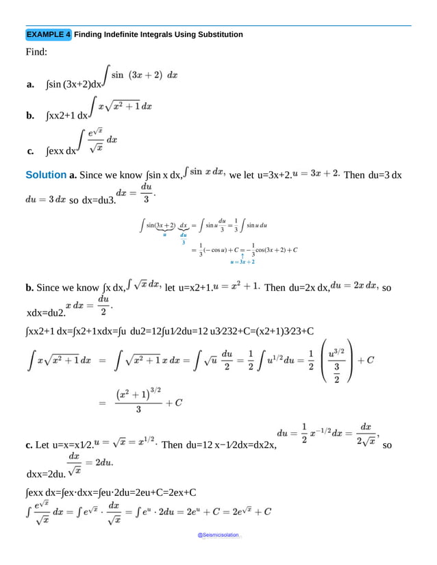
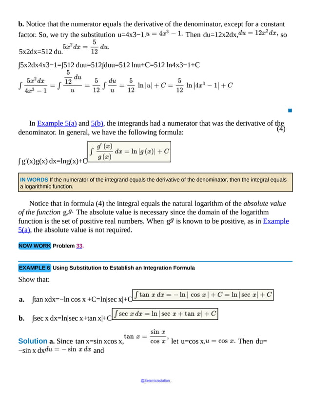
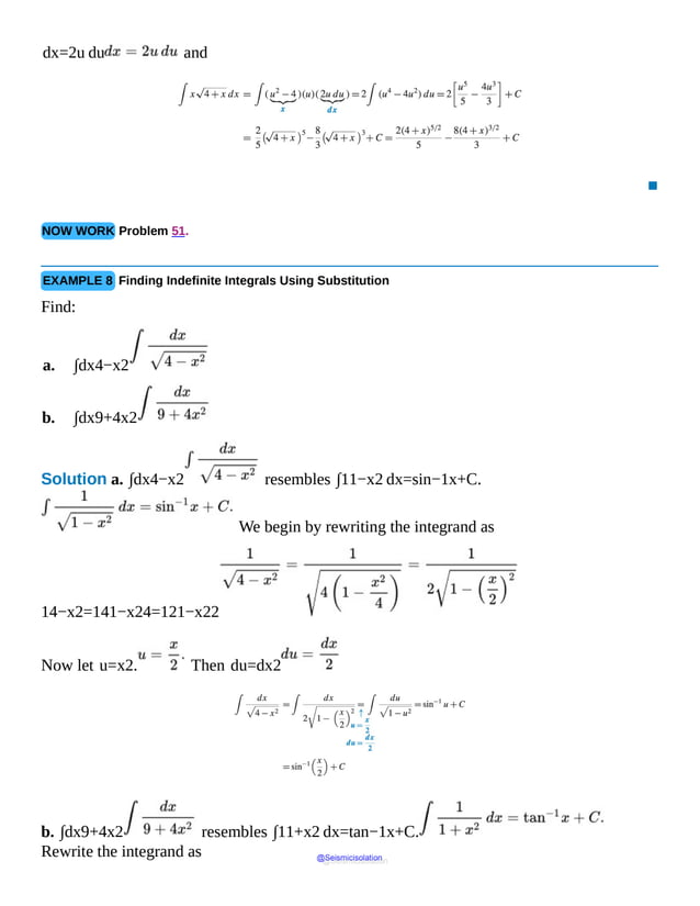
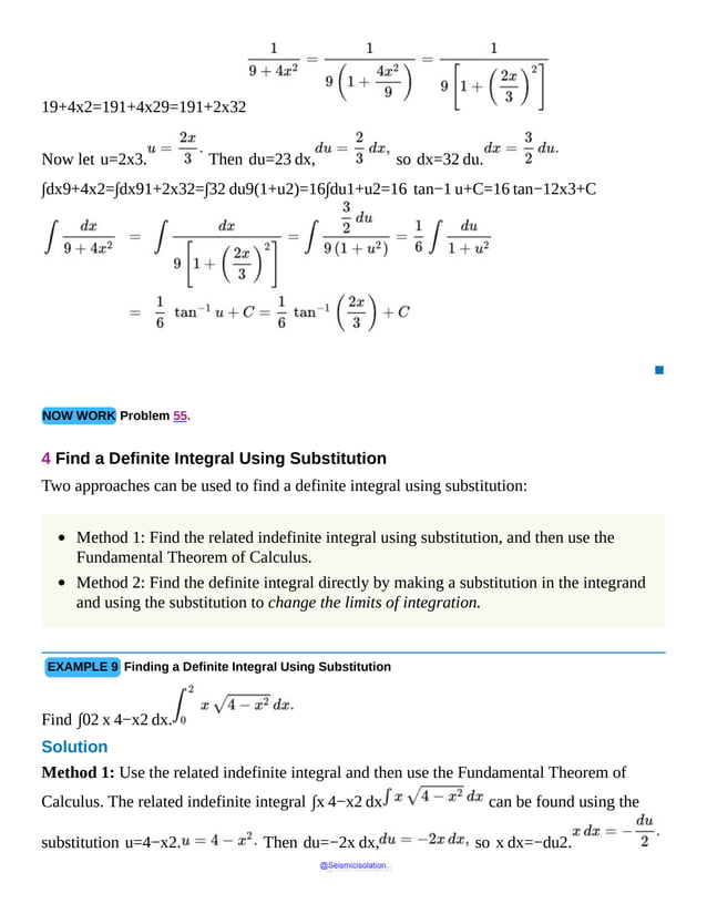
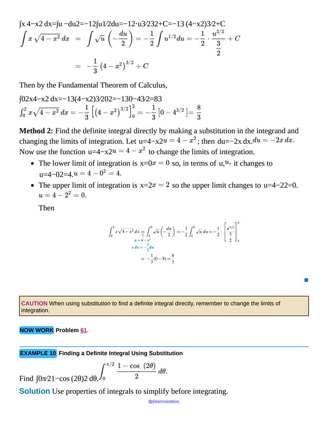
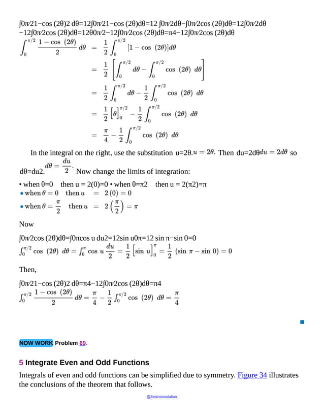
1096. (5)
Figure 34
The
graphs
show
curves
for
even
function
f
of
x
and
odd
function
g
of
x
respectively
under
the
closed
interval
[minus
a,
a].
RECALL A function f is even if f(−x)=f(x) and is odd if f(−x)=−f(x) for all
x in the domain of f.
THEOREM The Integrals of Even and Odd Functions
Let a function f be continuous on a closed interval [−a,a], a>0.
If f is an even function, then
∫−aaf(x)dx=2∫0af(x)dx
If f is an odd function, then
∫−aaf(x)dx=0
The property for even functions is proved here; the proof for odd functions is left as an
exercise. See Problem 135.
Proof f is an even function: Since f is continuous on the closed interval [−a,a],
a>0, and 0 is in the interval −a,a, we have
∫−aaf(x)dx=∫−a0f(x)dx+∫0af(x)dx=−∫0−af(x)dx+∫0af(x)dx
In −∫0−af(x)dx, we use the substitution u=−x. Then du=−dx.
Also, if x=0, then u=0, and if x=−a, then u=a.
@Seismicisolation
@Seismicisolation

1097. Therefore,
Combining (5) and (6), we obtain
∫−aaf(x)dx=∫0af(x)dx+∫0af(x)dx=2∫0af(x)dx
▪
To use the theorem involving even or odd functions, three conditions must be met:
The function f must be even or odd.
The function f must be continuous on the closed interval [−a,a], a>0.
The limits of integration must be −a and a, a>0.
EXAMPLE 11 Integrating an Even or Odd Function
Find:
a. ∫−33(x7−4x3+x)dx
b. ∫−22(x4−x2+3)dx
Solution a. If f(x)=x7−4x3+x, then
f(−x)=(−x)7−4(−x)3+(−x)=−(x7−4x3+x)=−f(x)
Since f is an odd function,
∫−33(x7−4x3+x)dx=0
b. If g(x)=x4−x2+3, then g(−x)=(−x)4−(−x)2+3=x4−x2+3=g(x).
Since g is an even function,
∫−22(x4−x2+3)dx=2∫02(x4−x2+3)dx=2x55−x33+3x02=2325−83+6=29215
@Seismicisolation
@Seismicisolation

1098. ▪
NOW WORK Problems 79 and 81.
EXAMPLE 12 Using Properties of Integrals
If f is an even function and ∫02f(x)dx=−6 and ∫−50f(x)dx=8,
find ∫25f(x)dx.
Solution ∫25f(x)dx=∫20f(x)dx+∫05f(x)dx
Now ∫20f(x)dx=−∫02f(x)dx=6.
Since f is even, ∫05f(x)dx= ∫−50f(x)dx=8. Then
∫25f(x)dx=∫20f(x)dx+∫05f(x)dx=6+8=14
▪
NOW WORK Problem 87.
5.5 Assess Your Understanding
Concepts and Vocabulary
1. ddx ∫f(x)dx= ________
2. True or False If k is a constant, then ∫kf(x)dx=∫k dx⋅∫f(x)dx
3. If a is a real number, a≠−1, then ∫xadx= ________.
4. True or False When finding the indefinite integral of a function f, a constant of
@Seismicisolation
@Seismicisolation

1099. integration C is added to the result because ∫f(x)dx denotes all the
antiderivatives of f.
5. If the substitution u=2x+3 is used with ∫sin (2x+3)dx, the
result is ∫ ______ du.
6. True or False If the substitution u=x2+3 is used with ∫01x(x2+3)3dx,
then ∫01x(x2+3)3dx=12∫01u3du.
7. Multiple Choice ∫−44x3dx=[(a)128(b)4(c)0(d)64]
8. True or False ∫05x2dx=12∫−55x2dx
Skill Building
In Problems 9–20, find each indefinite integral.
9. ∫x2⁄3dx
10. ∫t−4dt
11. ∫11−x2 dx
12. ∫11+x2 dx
13. ∫5x2+2xex−1x dx
14. ∫xex+1x dx
15. ∫tan xcos x dx
16. ∫1sin2x dx
@Seismicisolation
@Seismicisolation

1100. 17. ∫251−x2 dx
18. ∫−4xx2−1 dx
19. ∫sinh tdt
20. ∫cosh tdt
In Problems 21–26, find each indefinite integral using the given substitution.
21. ∫e3x+1dx ; let u=3x+1
22. ∫dxx ln x ; let u=ln x
23. ∫(1−t2)6tdt; let u=(1−t2)
24. ∫sin5x cos xdx; let u=sin x
25. ∫x2dx1−x6 ; let u=x3
26. ∫e−x6+e−xdx; let u=6+e−x
In Problems 27–60, find each indefinite integral.
27. ∫sin (3x)dx
28. ∫x sin x2dx
29. ∫sin x cos2xdx
@Seismicisolation
@Seismicisolation

1101. 30. ∫tan2 x sec2 xdx
31. ∫e1⁄xx2 dx
32. ∫ex3x23 dx
33. ∫xdxx2−1
34. ∫5xdx1−x2
35. ∫ex1+ex dx
36. ∫dxx (ln x)7
37. ∫1x(1+x)4 dx
38. ∫dxx(1+x)
39. ∫3exex−14 dx
40. ∫[ln(5x)]3x dx
41. ∫cos xdx2 sin x−1
42. ∫cos (2x)dxsin (2x)
43. ∫sec (5x)dx
@Seismicisolation
@Seismicisolation

1102. 44. ∫tan (2x)dx
45. ∫tan x sec2 xdx
46. ∫(2+3 cot x)3⁄2 csc2xdx
47. ∫sin xcos2x dx
48. ∫cos xsin2x dx
49. ∫sin x⋅ecos xdx
50. ∫sec2 x⋅etan xdx
51. ∫xx+3 dx
52. ∫x4−x dx
53. ∫[sin x+cos (3x)]dx
54. ∫[x2+3x+2]dx
55. ∫dxx2+25
56. ∫cos x1+sin2x dx
57. ∫dx9−x2
58. ∫dx16−9x2
@Seismicisolation
@Seismicisolation

1103. 59. ∫sinh x cosh xdx
60. ∫sech2x tanh xdx
In Problems 61–68, find each definite integral two ways:
a. By finding the related indefinite integral and then using the Fundamental Theorem of
Calculus;
b. By making a substitution in the integrand and using the substitution to change the
limits of integration.
c. Which method did you prefer? Why?
61. ∫−20x(x2+3)2 dx
62. ∫−11(x2−1)5xdx
63. ∫01x2ex3+1dx
64. ∫01xex2−2dx
65. ∫16xx+3 dx
66. ∫26x2x−2 dx
67. ∫02x⋅32x2dx
68. ∫01x⋅10−x2dx
In Problems 69–78, find each definite integral.
69. ∫131x21−1x dx
@Seismicisolation
@Seismicisolation

1104. 70. ∫0π⁄4sin (2x)5−2 cos (2x) dx
71. ∫02e2xe2x+1 dx
72. ∫13e3xe3x−1 dx
73. ∫23dxx ln x
74. ∫23dxx(ln x)2
75. ∫0πexcos (ex)dx
76. ∫0πe−xcos (e−x)dx
77. ∫01xdx1+x4
78. ∫01ex1+e2x dx
In Problems 79–86, use properties of even and odd functions to find each integral.
79. ∫−22(x2−4)dx
80. ∫−11(x3−2x)dx
81. ∫−π⁄2π⁄213 sin θdθ
82. ∫−π⁄4π⁄4sec2 xdx
83. ∫−1131+x2 dx
@Seismicisolation
@Seismicisolation

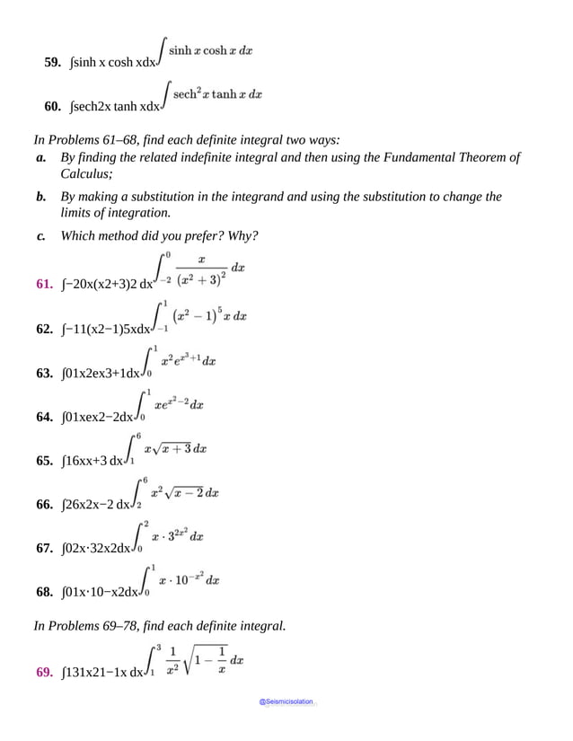
1105. 84. ∫−55(x1⁄3+x)dx
85. ∫−55|2x|dx
86. ∫−11[| x|−3]dx
87. If f is an odd function and ∫03f(x)dx=6 and ∫35f(x)dx=2,
find ∫−35f(x)dx.
88. If f is an odd function and ∫−510f(x)dx=8, find ∫510f(x)dx.
89. If f is an even function and ∫04f(x)dx=−2 and ∫06f(x)dx=6,
find ∫−46f(x)dx.
90. If f is an even function and ∫−30f(x)dx=4 and ∫−50f(x)dx=1,
find ∫35f(x)dx.
Applications and Extensions
In Problems 91 and 92, find each indefinite integral by
a. Using substitution.
b. Expanding the integrand.
91. ∫(x+1)2dx
92. ∫(x2+1)2xdx
In Problems 93 and 94, find each integral three ways:
a. By using substitution.
b. By using even-odd properties of the definite integral.
c. By using trigonometry to simplify the integrand before integrating.
d. Verify the results are equivalent.
@Seismicisolation
@Seismicisolation

1106. 93. ∫−π⁄2π⁄2cos (2x+π)dx
94. ∫−π⁄4π⁄4sin (7θ−π)dθ
95. Area Find the area under the graph of f(x)=x22x+1 from 0 to 4.
96. Area Find the area under the graph of f(x)=x(x2+1)2 from 0 to 2.
97. Area Find the area under the graph of y=13x2+1 from x=0 to x=1.
98. Area Find the area under the graph of y=1xx2−4 from x=3 to x=4.
99. Area Find the area under the graph of the catenary,
y=a cosh xa+b−a
from x=0 to x=a.
100. Area Find b so that the area under the graph of
y=(x+1)x2+2x+4
is 563 for 0≤x≤b.
101. Average Value Find the average value of y=tanx on the interval 0,π4.
102. Average Value Find the average value of y=sec x on the interval 0,π4.
103. If ∫02f(x−3)dx=8, find ∫−3−1f(x)dx.
104. If ∫−21f(x+1)dx=52, find ∫−12f(x)dx.
105. If ∫04gx2dx=8, find ∫02g(x)dx.
@Seismicisolation
@Seismicisolation

1107. 106. If ∫01g(3x)dx=6, find ∫03g(x)dx.
In Problems 107–112, find each integral. (Hint: Begin by using a Change of Base formula.)
107. ∫dxxlog10x
108. ∫dxxlog3x5
109. ∫10100dxxlogx
110. ∫832dxxlog2x
111. ∫39dxxlog3x
112. ∫10100dxxlog5x
113. If ∫1bt2(5t3−1)1⁄2dt=3845, find b.
114. If ∫a3t9−t2dt=6, find a.
In Problems 115–128, find each integral.
115. ∫x+1x2+1 dx
116. ∫2x−31+x2 dx
117. ∫2x2+3−4x+96xx2+3+2x2dx
118. ∫(z2+1)4−3z(z2+1)3dz
119. ∫x+4x3x dx
@Seismicisolation
@Seismicisolation

1108. 120. ∫zdzz+z2+4
121. ∫t4+tt dt
122. ∫01x+1x2+3 dx
123. ∫32x+1dx
124. ∫23x+5dx
125. ∫sin x4−cos2x dx
126. ∫sec2 xdx1−tan2x
127. ∫01(z2+5)(z3+15z−3)196−(z3+15z−3)2 dz
128. ∫217dxx−1+(x−1)5⁄4
129. Use an appropriate substitution to show that
∫01xm(1−x)n dx=∫01xn(1−x)m dx
where m, n are positive integers.
130. Find ∫−11f(x)dx, for the function given below
f(x)=x+1ifx<0cos (πx)ifx≥0
131. If f is continuous on [a,b], show that
@Seismicisolation
@Seismicisolation

1109. ∫abf(x)dx=∫abf(a+b−x)dx
132. If ∫01f(x)dx=2, find
a. ∫00.5f(2x)dx
b. ∫03f13 xdx
c. ∫01⁄5f(5x)dx
d. Find the upper and lower limits of integration so that
∫abfx4dx=8
e. Generalize (d) so that ∫abf(kx)dx=1k⋅2 for k>0.
133. If ∫02f(s)ds=5, find
a. ∫−11f(s+1)ds
b. ∫−3−1f(s+3)ds
c. ∫46f(s−4)ds
d. Find upper and lower limits of integration so that
∫abf(s−2)ds=5
e. Generalize (d) so that ∫abf(s−k)ds=5 for k>0.
134. Find ∫0b|2x|dx for any real number b.
135. If f is an odd function, show that ∫−aaf(x)dx=0.
136. Find the constant k, where 0≤k≤3, for which
@Seismicisolation
@Seismicisolation

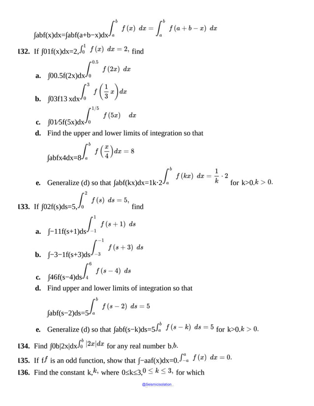
1110. ∫03xx2+16 dx=3kk2+16
137. If n is a positive integer, for what number c>0 is
∫0cxn−1 dx=1n?
138. If f is a continuous function defined on the interval [0,1], show that
∫0πx f(sin x)dx=π2∫0πf(sin x)dx
139. Prove that ∫csc xdx=lncsc x−cotx+C. [Hint: Multiply
and divide by (csc x−cot x). ]
140. Describe a method for finding ∫ab|f(x)|dx in terms of F(x)=∫f(x)dx
when f has finitely many zeros.
141. Find ∫a+bxn dx where a and b are real numbers, b≠0, and n≥2
is an integer.
142. If f is continuous for all x, which of the following integrals have the same value?
a. ∫abf(x)dx
b. ∫0b−af(x+a)dx
c. ∫a+cb+cf(x+c)dx
143. Area Let f(x)=ksin (kx), where k is a positive constant.
a. Find the area of the region under one arch of the graph of f.
b. Find the area of the triangle formed by the x -axis and the tangent lines to one arch
of f at the points where the graph of f crosses the x -axis.
144. Prove that ∫[f(x)+g(x)]dx=∫f(x)dx+∫g(x)dx.
145. Derive the integration formula ∫axdx=axln a+C, a>0, a≠1.
(Hint: Begin with the derivative of y=ax. )
@Seismicisolation
@Seismicisolation

1111. 146. Use the formula from Problem 145 to find
a. ∫2xdx
b. ∫3xdx
147. Electric Potential The electric field strength a distance z from the axis of a ring of
radius R carrying a charge Q is given by the formula
E(z)=Qz(R2+z2)3⁄2
If the electric potential V is related to E by E=−dVdz, what is V(z)
?
148. Impulse During a Rocket Launch The impulse J due to a force F is the product of
the force times the amount of time t for which the force acts. When the force varies
over time,
J=∫t1t2f(t)dt.
We can model the force acting on a rocket during launch by an exponential function
F(t)=Aebt, where A and b are constants that depend on the
characteristics of the engine. At the instant lift-off occurs (t=0 ), the force must
equal the weight of the rocket.
@Seismicisolation
@Seismicisolation

1112. a. Suppose the rocket weighs 25,000 N (a mass of about 2500kg or a weight
of 5500lb ), and 30 s after lift-off the force acting on the rocket equals twice
the weight of the rocket. Find A and b.
b. Find the impulse delivered to the rocket during the first 30 seconds after the launch.
Challenge Problems
149. Air Resistance on a Falling Object If an object of mass m is dropped, the air
resistance on it when it has speed v can be modeled as Fair=−kv, where the
constant k depends on the shape of the object and the condition of the air. The minus
sign is necessary because the direction of the force is opposite to the velocity. Using
Newton’s Second Law of Motion, this force leads to a downward acceleration a(t)=ge
−kt⁄m. (You are asked to prove this in Problem 150.) Using the equation
for a(t), find:
a. v(t), if the object starts from rest v0=v(0)=0, with the positive
direction downward.
b. s(t), if the object starts from the position s0=s(0)=0, with the
positive direction downward.
c. What limits do a(t), v(t), and s(t) approach if the object falls for a
very long time (t→∞ )? Interpret each result and explain if it is physically
reasonable.
d. Graph a=a(t), v=v(t), s=s(t). Do the graphs support the
conclusions obtained in part (c)? Use g=9.8 m⁄s2, k=5, and
m=10 kg.
150. Air Resistance on a Falling Object (Refer to Problem 149.) If an object of mass m
is dropped, the air resistance on it when it has speed v can be modeled as
Fair=−kv
where the constant k depends on the shape of the object and the condition of the air.
The minus sign is necessary because the direction of the force is opposite to the
velocity. Using Newton’s Second Law of Motion, show that the downward acceleration
of the object is
a(t)=ge−kt⁄m
where g is the acceleration due to gravity.
(Hint: The velocity of the object obeys the differential equation
@Seismicisolation
@Seismicisolation

1113. m dvdt=mg−kv
Solve the differential equation for v and use the fact that ma=mg−kv. )
151. Find ∫x6+3x4+3x2+x+1(x2+1)2 dx.
152. Find ∫x4x+x3dx.
153. Find ∫3x+2xx+1dx.
154. Find ∫dx(x ln x)[ln(ln x)].
155.
a. Find y′ if y=lntanx2+π4.
b. Use the result to show that
∫ sec xdx=lntan x2+π4+C
c. Show that lntan x2+π4=ln sec x+tan x.
156.
a. Find y′ if y=xsin−1x+1−x2.
b. Use the result to show that
∫sin−1xdx=x sin−1x+1−x2+C
157.
a. Find y′ if y=12 xa2−x2+12 a2sin−1xa, a>0.
b. Use the result to show that
∫a2−x2 dx=12 xa2−x2+12 a2sin−1xa+C
158. a. Find y′ if y=ln csc x−cot x.
b. Use the result to show that
∫cscxdx=ln csc x−cot x+C
@Seismicisolation
@Seismicisolation

1114. 159. Gudermannian Function
a. Graph y=gd(x)=ta