This document summarizes key exercises from Chapter 1 of a textbook on systems of linear equations and matrices. It provides examples of determining whether equations are linear or nonlinear, constructing augmented matrices to represent systems of linear equations, row reducing matrices to solve systems, and checking solutions. Matrix row echelon form and reduced row echelon form are discussed. Solutions are provided for sample systems of linear equations.
![Chapter 1: Systems of Linear Equations and Matrices SSM: Elementary Linear Algebra
2
(b)
3 0 5
2
7 3
1 4
0 7
2 1
⎡ ⎤
−
⎢ ⎥
−
⎢ ⎥
−
⎢ ⎥
⎣ ⎦
corresponds to
1 3
1 2 3
2 3
3 2 5
7 4 3
2 7
.
x x
x x x
x x
− =
+ + = −
− + =
(c) 7 3 5
2 1
0
1 2 4 1
⎡ ⎤
−
⎢ ⎥
⎣ ⎦
corresponds to
1 2 3 4
1 2 3
7 2 3 5
2 4 1
x x x x
x x x
+ + − =
+ + =
.
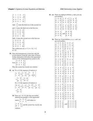
(d)
0 0 0 7
1
0 0 0
1 2
0 0 0 3
1
0 0 0 1 4
⎡ ⎤
⎢ ⎥
−
⎢ ⎥
⎢ ⎥
⎢ ⎥
⎣ ⎦
corresponds to
1
2
3
4
7
2
3
4
.
x
x
x
x
=
= −
=
=
13. (a) The augmented matrix for 1
1
1
2 6
3 8
9 3
x
x
x
− =
=
= −
is
6
2
3 8
9 3
.
⎡ ⎤
−
⎢ ⎥
⎢ ⎥
−
⎢ ⎥
⎣ ⎦
(b) The augmented matrix for
1 2 3
2 3
6 3 4
5 1
x x x
x x
− + =
− =
is 6 3
1 4
0 5 1 1
.
⎡ ⎤
−
⎢ ⎥
⎣ − ⎦
(c) The augmented matrix for
2 4 5
1 2 3
1 2 3 4 5
2 3 0
3 1
6 2 2 3 6
x x x
x x x
x x x x x
− + =
− − + = −
+ − + − =
is
0 0 3 0
2 1
3 0 0
1 1 1
6 3 6
2 1 2
.
⎡ ⎤
−
⎢ ⎥
− − −
⎢ ⎥
−
−
⎢ ⎥
⎣ ⎦
(d) The augmented matrix for 1 5 7
x x
− = is
[1 0 0 0 −1 7].
15. If (a, b, c) is a solution of the system, then
2
1 1 1,
ax bx c y
+ + = 2
2 2 2,
ax bx c y
+ + = and
2
3 3 3
ax bx c y
+ + = which simply means that the
points are on the curve.
17. The solutions of 1 2
x kx c
+ = are 1 ,
x c kt
= −
2
x t
= where t is any real number. If these
satisfy 1 2 ,
x lx d
+ = then c − kt + lt = d or
c − d = (k − l) t for all real numbers t. In
particular, if t = 0, then c = d, and if t = 1, then
k = l.
True/False 1.1
(a) True; 1 2 0
n
x x x
= = = = will be a solution.
(b) False; only multiplication by nonzero constants
is acceptable.
(c) True; if k = 6 the system has infinitely many
solutions, while if k ≠ 6, the system has no
solution.
(d) True; the equation can be solved for one variable
in terms of the other(s), yielding parametric
equations that give infinitely many solutions.
(e) False; the system 3 5 7
2 9 20
6 10 14
x y
x y
x y
− = −
+ =
− = −
has the
solution x = 1, y = 2.
(f) False; multiplying an equation by a nonzero
constant c does not change the solutions of the
system.
(g) True; subtracting one equation from another is
the same as multiplying an equation by −1 and
adding it to another.
(h) False; the second row corresponds to the
equation 1 2
0 0 1
x x
+ = − or 0 = −1 which is false.
Section 1.2
Exercise Set 1.2
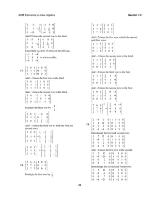
1. (a) The matrix is in both row echelon and
reduced row echelon form.
(b) The matrix is in both row echelon and
reduced row echelon form.](https://image.slidesharecdn.com/elementary-linear-algebra-chapter1-220420115526/85/Elementary-linear-algebra-chapter-1-pdf-2-320.jpg)
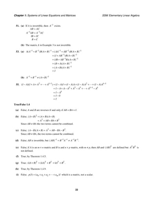
![SSM: Elementary Linear Algebra Section 1.3
13
(k)
1 3 12 2 8
3 1 1
tr 2 tr 4 1 2 2 2
0 2 1
2 5 6 4 6
1 3 3 0 1 1 3 2 1 1 3 1 12 2 8
tr 4 3 1 0 4 1 1 2 4 1 1 1 2 2 2
2 3 5 0 2 1 5 2 2 1 5 1 6 4 6
( )
( ) ( ) ( ) ( ) ( ) ( )
( ) ( ) ( ) ( ) ( ) ( )
( ) ( ) ( ) ( ) ( ) ( )
T T T
C A E
⎛ ⎞
−
⎡ ⎤ ⎡ ⎤
−
⎡ ⎤
⎜ ⎟
⎢ ⎥ ⎢ ⎥
+ = +
⎢ ⎥
⎜ ⎟
⎢ ⎥ ⎢ ⎥
⎣ ⎦
⎜ ⎟
⎣ ⎦ ⎣ ⎦
⎝ ⎠
⋅ + ⋅ − ⋅ + ⋅ ⋅ + ⋅ −
⎡ ⎤ ⎡
⎢ ⎥ ⎢
= ⋅ + ⋅ − ⋅ + ⋅ ⋅ + ⋅ +
⎢ ⎥
⋅ + ⋅ − ⋅ + ⋅ ⋅ + ⋅
⎣ ⎦ ⎣
3 5 4 12 2 8
tr 12 2 5 2 2 2
6 8 7 6 4 6
15 3 12
tr 14 0 7
12 12 13
15 0 13
28
⎛ ⎞
⎤
⎜ ⎟
⎥
⎜ ⎟
⎢ ⎥
⎜ ⎟
⎦
⎝ ⎠
⎛ ⎞
−
⎡ ⎤ ⎡ ⎤
⎜ ⎟
⎢ ⎥ ⎢ ⎥
= − +
⎜ ⎟
⎢ ⎥ ⎢ ⎥
⎜ ⎟
⎣ ⎦ ⎣ ⎦
⎝ ⎠
⎛ ⎞
⎡ ⎤
⎜ ⎟
⎢ ⎥
=
⎜ ⎟
⎢ ⎥
⎜ ⎟
⎣ ⎦
⎝ ⎠
= + +
=
(l)
6 1 3 1 3 3 0
tr tr 1 1 2 4 1 1 2
4 1 3 2 5 1 1
6 1 1 4 3 2 6 3 1 1 3 5
tr 1 1 1 4 2 2 1 3 1 1 2 5
4 1 1 4 3 2 4 3 1 1 3 5
(( ) )
( ) ( ) ( ) ( ) ( ) ( )
( ) ( ) ( ) ( ) ( ) ( )
( ) ( ) ( ) ( ) ( ) ( )
T
T T
EC A
⎛ ⎞
⎛ ⎞
⎡ ⎤ ⎡ ⎤ ⎡ ⎤
⎜ ⎟
⎜ ⎟
⎢ ⎥ ⎢ ⎥ ⎢ ⎥
= − −
⎜ ⎟
⎜ ⎟
⎢ ⎥ ⎢ ⎥ ⎢ ⎥
⎜ ⎟
⎜ ⎟
⎣ ⎦ ⎣ ⎦ ⎣ ⎦
⎝ ⎠
⎝ ⎠
⎛ ⋅ + ⋅ + ⋅ ⋅ + ⋅ + ⋅
⎡ ⎤
⎜ ⎢ ⎥
= − ⋅ + ⋅ + ⋅ − ⋅ + ⋅ + ⋅
⎢ ⎥
⋅ + ⋅ + ⋅ ⋅ + ⋅ + ⋅
⎣ ⎦
⎝
3 0
1 2
1 1
16 34 3 0
tr 7 8 1 2
14 28 1 1
3 0
16 7 14
tr 1 2
34 8 28
1 1
16 3 7 1 14 1 16
tr
34 34 0
( ) ( ) ( ) (
( ( )
T
T
⎛ ⎞
⎞ ⎡ ⎤
⎜ ⎟
⎟ ⎢ ⎥
−
⎜ ⎟
⎜ ⎟ ⎢ ⎥
⎜ ⎟
⎜ ⎟
⎣ ⎦
⎠
⎝ ⎠
⎛ ⎞
⎛ ⎞
⎡ ⎤ ⎡ ⎤
⎜ ⎟
⎜ ⎟
⎢ ⎥ ⎢ ⎥
= −
⎜ ⎟
⎜ ⎟
⎢ ⎥ ⎢ ⎥
⎜ ⎟
⎜ ⎟
⎣ ⎦ ⎣ ⎦
⎝ ⎠
⎝ ⎠
⎛ ⎞
⎡ ⎤
⎡ ⎤
⎜ ⎟
⎢ ⎥
= −
⎢ ⎥
⎜ ⎟
⎢ ⎥
⎣ ⎦
⎜ ⎟
⎣ ⎦
⎝ ⎠
⋅ − ⋅ + ⋅ ⋅0)+ (7⋅2) + (14⋅1)
=
⋅3) −(8⋅1) + (28⋅1) ⋅ 8 2 28 1
55 28
tr
122 44
55 44
99
( ) ( )
⎛ ⎞
⎡ ⎤
⎜ ⎟
⎢ ⎥
+ ⋅ + ⋅
⎣ ⎦
⎝ ⎠
⎛ ⎞
⎡ ⎤
= ⎜ ⎟
⎢ ⎥
⎣ ⎦
⎝ ⎠
= +
=
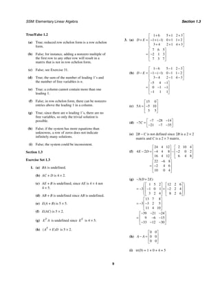
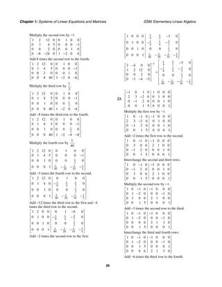
7. (a) The first row of AB is the first row of A times B.
1
6 2 4
3 2 7 0 1 3
7 7 5
18 0 49 6 2 49 12 6 35
67 41 41
[ ] [ ]
[ ]
[ ]
B
−
⎡ ⎤
⎢ ⎥
= −
⎢ ⎥
⎣ ⎦
= + + − − + − +
=
a](https://image.slidesharecdn.com/elementary-linear-algebra-chapter1-220420115526/85/Elementary-linear-algebra-chapter-1-pdf-13-320.jpg)
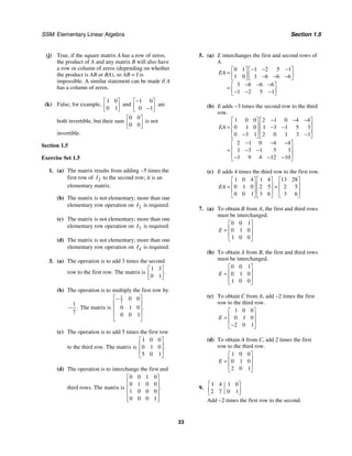
![Chapter 1: Systems of Linear Equations and Matrices SSM: Elementary Linear Algebra
14
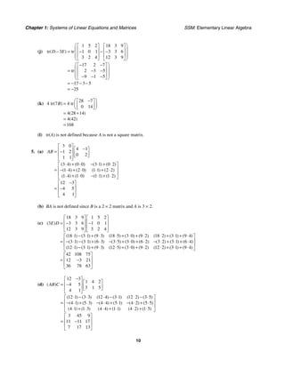
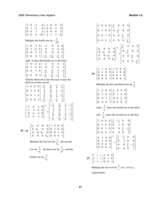
(b) The third row of AB is the third row of A
times B.
3
6 2 4
0 4 9 0 1 3
7 7 5
0 0 63 0 4 63 0 12 45
63 67 57
[ ]
[ ]
[ ]
[ ]
B
−
⎡ ⎤
⎢ ⎥
=
⎢ ⎥
⎣ ⎦
= + + + + + +
=
a
(c) The second column of AB is A times the
second column of B.
2
3 2 7 2
6 5 4 1
0 4 9 7
6 2 49
12 5 28
0 4 63
41
21
67
[ ]
A
− −
⎡ ⎤ ⎡ ⎤
⎢ ⎥ ⎢ ⎥
=
⎢ ⎥ ⎢ ⎥
⎣ ⎦ ⎣ ⎦
− − +
⎡ ⎤
⎢ ⎥
= − + +
⎢ ⎥
+ +
⎣ ⎦
⎡ ⎤
⎢ ⎥
=
⎢ ⎥
⎣ ⎦
b
(d) The first column of BA is B times the first
column of A.
1
6 2 4 3
0 1 3 6
7 7 5 0
18 12 0
0 6 0
21 42 0
6
6
63
[ ]
B
−
⎡ ⎤ ⎡ ⎤
⎢ ⎥ ⎢ ⎥
=
⎢ ⎥ ⎢ ⎥
⎣ ⎦ ⎣ ⎦
− +
⎡ ⎤
⎢ ⎥
= + +
⎢ ⎥
+ +
⎣ ⎦
⎡ ⎤
⎢ ⎥
=
⎢ ⎥
⎣ ⎦
a
(e) The third row of AA is the third row of A
times A.
3
3 2 7
0 4 9 6 5 4
0 4 9
0 24 0 0 20 36 0 16 81
24 56 97
[ ]
[ ]
[ ]
[ ]
A
−
⎡ ⎤
⎢ ⎥
=
⎢ ⎥
⎣ ⎦
= + + + + + +
=
a
(f) The third column of AA is A times the third
column of A.
3
3 2 7 7
6 5 4 4
0 4 9 9
21 8 63
42 20 36
0 16 81
76
98
97
[ ]
A
−
⎡ ⎤ ⎡ ⎤
⎢ ⎥ ⎢ ⎥
=
⎢ ⎥ ⎢ ⎥
⎣ ⎦ ⎣ ⎦
− +
⎡ ⎤
⎢ ⎥
= + +
⎢ ⎥
+ +
⎣ ⎦
⎡ ⎤
⎢ ⎥
=
⎢ ⎥
⎣ ⎦
a
9. (a)
3 12 76
48 29 98
24 56 97
AA
−
⎡ ⎤
⎢ ⎥
=
⎢ ⎥
⎣ ⎦
3 3 2
48 3 6 6 5
24 0 4
− −
⎡ ⎤ ⎡ ⎤ ⎡ ⎤
⎢ ⎥ ⎢ ⎥ ⎢ ⎥
= +
⎢ ⎥ ⎢ ⎥ ⎢ ⎥
⎣ ⎦ ⎣ ⎦ ⎣ ⎦
12 3 2 7
29 2 6 5 5 4 4
56 0 4 9
−
⎡ ⎤ ⎡ ⎤ ⎡ ⎤ ⎡ ⎤
⎢ ⎥ ⎢ ⎥ ⎢ ⎥ ⎢ ⎥
= − + +
⎢ ⎥ ⎢ ⎥ ⎢ ⎥ ⎢ ⎥
⎣ ⎦ ⎣ ⎦ ⎣ ⎦ ⎣ ⎦
76 3 2 7
98 7 6 4 5 9 4
97 0 4 9
−
⎡ ⎤ ⎡ ⎤ ⎡ ⎤ ⎡ ⎤
⎢ ⎥ ⎢ ⎥ ⎢ ⎥ ⎢ ⎥
= + +
⎢ ⎥ ⎢ ⎥ ⎢ ⎥ ⎢ ⎥
⎣ ⎦ ⎣ ⎦ ⎣ ⎦ ⎣ ⎦
(b)
64 14 38
21 22 18
77 28 74
BB
⎡ ⎤
⎢ ⎥
=
⎢ ⎥
⎣ ⎦
64 6 4
21 6 0 7 3
77 7 5
⎡ ⎤ ⎡ ⎤ ⎡ ⎤
⎢ ⎥ ⎢ ⎥ ⎢ ⎥
= +
⎢ ⎥ ⎢ ⎥ ⎢ ⎥
⎣ ⎦ ⎣ ⎦ ⎣ ⎦
14 6 2 4
22 2 0 1 1 7 3
28 7 7 5
−
⎡ ⎤ ⎡ ⎤ ⎡ ⎤ ⎡ ⎤
⎢ ⎥ ⎢ ⎥ ⎢ ⎥ ⎢ ⎥
= − + +
⎢ ⎥ ⎢ ⎥ ⎢ ⎥ ⎢ ⎥
⎣ ⎦ ⎣ ⎦ ⎣ ⎦ ⎣ ⎦
38 6 2 4
18 4 0 3 1 5 3
74 7 7 5
−
⎡ ⎤ ⎡ ⎤ ⎡ ⎤ ⎡ ⎤
⎢ ⎥ ⎢ ⎥ ⎢ ⎥ ⎢ ⎥
= + +
⎢ ⎥ ⎢ ⎥ ⎢ ⎥ ⎢ ⎥
⎣ ⎦ ⎣ ⎦ ⎣ ⎦ ⎣ ⎦
11. (a)
2 3 5
9 1 1
1 5 4
,
A
−
⎡ ⎤
⎢ ⎥
= −
⎢ ⎥
⎣ ⎦
1
2
3
,
x
x
x
⎡ ⎤
⎢ ⎥
=
⎢ ⎥
⎣ ⎦
x
7
1
0
⎡ ⎤
⎢ ⎥
= −
⎢ ⎥
⎣ ⎦
b
The equation is
1
2
3
2 3 5 7
9 1 1 1
1 5 4 0
.
x
x
x
− ⎡ ⎤
⎡ ⎤ ⎡ ⎤
⎢ ⎥
⎢ ⎥ ⎢ ⎥
− = −
⎢ ⎥
⎢ ⎥ ⎢ ⎥
⎣ ⎦ ⎣ ⎦
⎣ ⎦](https://image.slidesharecdn.com/elementary-linear-algebra-chapter1-220420115526/85/Elementary-linear-algebra-chapter-1-pdf-14-320.jpg)
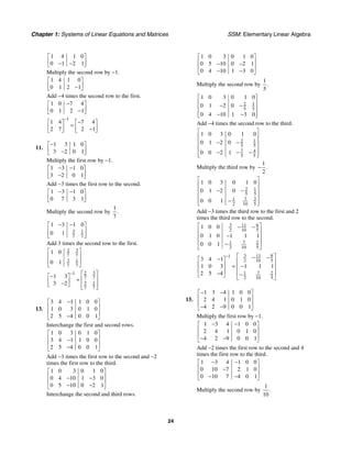
![SSM: Elementary Linear Algebra Section 1.3
15
(b)
4 0 3 1
5 1 0 8
2 5 9 1
0 3 1 7
,
A
−
⎡ ⎤
⎢ ⎥
−
= ⎢ ⎥
− −
⎢ ⎥
−
⎢ ⎥
⎣ ⎦
1
2
3
4
,
x
x
x
x
⎡ ⎤
⎢ ⎥
= ⎢ ⎥
⎢ ⎥
⎢ ⎥
⎣ ⎦
x
1
3
0
2
⎡ ⎤
⎢ ⎥
= ⎢ ⎥
⎢ ⎥
⎢ ⎥
⎣ ⎦
b
The equation is
1
2
3
4
4 0 3 1 1
5 1 0 8 3
2 5 9 1 0
0 3 1 7 2
.
x
x
x
x
⎡ ⎤
−
⎡ ⎤ ⎡ ⎤
⎢ ⎥
⎢ ⎥ ⎢ ⎥
−
⎢ ⎥ =
⎢ ⎥ ⎢ ⎥
− − ⎢ ⎥
⎢ ⎥ ⎢ ⎥
⎢ ⎥
−
⎢ ⎥ ⎢ ⎥
⎣ ⎦ ⎣ ⎦
⎣ ⎦
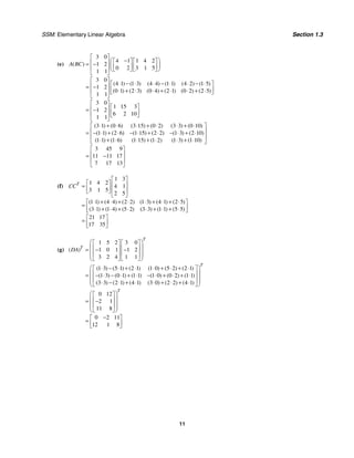
13. (a) The system is
1 2 3
1 2 3
2 3
5 6 7 2
2 3 0
4 3
x x x
x x x
x x
+ − =
− − + =
− =
(b) The system is
1 2 3
1 2
1 2 3
2
2 3 2
5 3 6 9
x x x
x x
x x x
+ + =
+ =
− − = −
15.
2
2
1 1 0
1 1 1 0 2 1
0 2 3 1
1 2 1 1
1
2 1
2 1
[ ]
[ ]
[ ]
[ ]
k
k
k
k k
k k k
k k
⎡ ⎤ ⎡ ⎤
⎢ ⎥ ⎢ ⎥
⎢ ⎥ ⎢ ⎥
−
⎣ ⎦ ⎣ ⎦
⎡ ⎤
⎢ ⎥
= + + −
⎢ ⎥
⎣ ⎦
= + + + −
= + +
The only solution of 2
2 1 0
k k
+ + = is k = −1.
17.
3 4 2
1 2 2
a d c
a b d c
−
⎡ ⎤ ⎡ ⎤
=
⎢ ⎥ ⎢ ⎥
− + + −
⎣ ⎦ ⎣ ⎦
gives the
equations
4
2 3
2 1
2
a
d c
d c
a b
=
− =
+ = −
+ = −
a = 4 ⇒ b = −6
d − 2c = 3, d + 2c = −1 ⇒ 2d = 2, d = 1
d = 1 ⇒ 2c = −2, c = −1
The solution is a = 4, b = −6, c = −1, d = 1.
19. The ij-entry of kA is .
ij
ka If 0
ij
ka = for all i, j
then either k = 0 or 0
ij
a = for all i, j, in which
case A = 0.
21. The diagonal entries of A + B are ,
ii ii
a b
+ so
11 11 22 22
11 22 11 22
tr
tr( tr
( )
( ) ( ) ( )
( ) ( )
) ( )
nn nn
nn nn
A B
a b a b a b
a a a b b b
A B
+
= + + + + + +
= + + + + + + +
= +
23. (a)
11
22
33
44
55
66
0 0 0 0 0
0 0 0 0 0
0 0 0 0 0
0 0 0 0 0
0 0 0 0 0
0 0 0 0 0
a
a
a
a
a
a
⎡ ⎤
⎢ ⎥
⎢ ⎥
⎢ ⎥
⎢ ⎥
⎢ ⎥
⎢ ⎥
⎢ ⎥
⎣ ⎦
(b)
11 12 13 14 15 16
22 23 24 25 26
33 34 35 36
44 45 46
55 56
66
0
0 0
0 0 0
0 0 0 0
0 0 0 0 0
a a a a a a
a a a a a
a a a a
a a a
a a
a
⎡ ⎤
⎢ ⎥
⎢ ⎥
⎢ ⎥
⎢ ⎥
⎢ ⎥
⎢ ⎥
⎢ ⎥
⎣ ⎦
(c)
11
21 22
31 32 33
41 42 43 44
51 52 53 54 55
61 62 63 64 65 66
0 0 0 0 0
0 0 0 0
0 0 0
0 0
0
a
a a
a a a
a a a a
a a a a a
a a a a a a
⎡ ⎤
⎢ ⎥
⎢ ⎥
⎢ ⎥
⎢ ⎥
⎢ ⎥
⎢ ⎥
⎢ ⎥
⎣ ⎦
(d)
11 12
21 22 23
32 33 34
43 44 45
54 55 56
65 66
0 0 0 0
0 0 0
0 0 0
0 0 0
0 0 0
0 0 0 0
a a
a a a
a a a
a a a
a a a
a a
⎡ ⎤
⎢ ⎥
⎢ ⎥
⎢ ⎥
⎢ ⎥
⎢ ⎥
⎢ ⎥
⎢ ⎥
⎣ ⎦
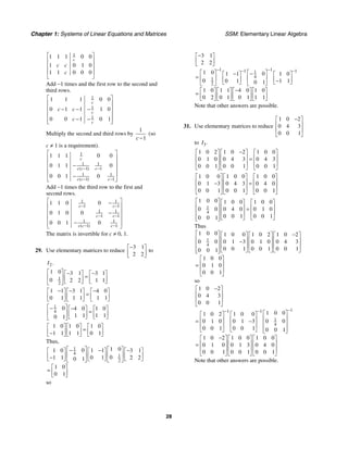
25. 1 1 1 2
2 2 2
1 1
0 1
x x x x
f
x x x
+
⎛ ⎞ ⎡ ⎤ ⎛ ⎞
⎡ ⎤
= =
⎜ ⎟ ⎜ ⎟
⎢ ⎥
⎢ ⎥
⎣ ⎦
⎝ ⎠ ⎣ ⎦ ⎝ ⎠
(a)
1 1 1 2
1 1 1
f
+
⎛ ⎞ ⎛ ⎞ ⎛ ⎞
= =
⎜ ⎟ ⎜ ⎟ ⎜ ⎟
⎝ ⎠ ⎝ ⎠ ⎝ ⎠
y
1
x
2
1
x f(x)](https://image.slidesharecdn.com/elementary-linear-algebra-chapter1-220420115526/85/Elementary-linear-algebra-chapter-1-pdf-15-320.jpg)
![Chapter 1: Systems of Linear Equations and Matrices SSM: Elementary Linear Algebra
16
(b)
2 2 0 2
0 0 0
f
+
⎛ ⎞ ⎛ ⎞ ⎛ ⎞
= =
⎜ ⎟ ⎜ ⎟ ⎜ ⎟
⎝ ⎠ ⎝ ⎠ ⎝ ⎠
y
1
x
2
1
f(x) = x
(c)
4 4 3 7
3 3 3
f
+
⎛ ⎞ ⎛ ⎞ ⎛ ⎞
= =
⎜ ⎟ ⎜ ⎟ ⎜ ⎟
⎝ ⎠ ⎝ ⎠ ⎝ ⎠
y
5
x
8
4
x f(x)
(d)
2 2 2 0
2 2 2
f
−
⎛ ⎞ ⎛ ⎞ ⎛ ⎞
= =
⎜ ⎟ ⎜ ⎟ ⎜ ⎟
− − −
⎝ ⎠ ⎝ ⎠ ⎝ ⎠
y
–1
x
2
x
–2
1
f(x)
27. Let [ ].
ij
A a
=
11 12 13 11 12 13
21 22 23 21 22 23
31 32 33 31 32 33
0
a a a a x a y a z
x
a a a y a x a y a z
z
a a a a x a y a z
x y
x y
+ +
⎡ ⎤ ⎡ ⎤
⎡ ⎤
⎢ ⎥ ⎢ ⎥
⎢ ⎥ = + +
⎢ ⎥ ⎢ ⎥
⎢ ⎥
+ +
⎢ ⎥ ⎢ ⎥
⎣ ⎦
⎣ ⎦ ⎣ ⎦
+
⎡ ⎤
⎢ ⎥
= −
⎢ ⎥
⎣ ⎦
The matrix equation yields the equations
11 12 13
21 22 23
31 32 33 0
a x a y a z x y
a x a y a z x y
a x a y a z
+ + = +
+ + = −
+ + =
.
For these equations to be true for all values of x,
y, and z it must be that 11 1,
a = 12 1,
a = 21 1,
a =
22 1,
a = − and 0
ij
a = for all other i, j. There is
one such matrix,
1 1 0
1 1 0
0 0 0
.
A
⎡ ⎤
⎢ ⎥
= −
⎢ ⎥
⎣ ⎦
29. (a) Both
1 1
1 1
⎡ ⎤
⎢ ⎥
⎣ ⎦
and
1 1
1 1
− −
⎡ ⎤
⎢ ⎥
− −
⎣ ⎦
are square roots
of
2 2
2 2
.
⎡ ⎤
⎢ ⎥
⎣ ⎦
(b) The four square roots of
5 0
0 9
⎡ ⎤
⎢ ⎥
⎣ ⎦
are
5 0
0 3
,
⎡ ⎤
⎢ ⎥
⎣ ⎦
5 0
0 3
,
⎡ ⎤
−
⎢ ⎥
⎣ ⎦
5 0
0 3
,
⎡ ⎤
⎢ ⎥
−
⎣ ⎦
and
5 0
0 3
.
⎡ ⎤
−
⎢ ⎥
−
⎣ ⎦
True/False 1.3
(a) True; only square matrices have main diagonals.
(b) False; an m × n matrix has m row vectors and
n column vectors.
(c) False; matrix multiplication is not commutative.
(d) False; the ith row vector of AB is found by
multiplying the ith row vector of A by B.
(e) True
(f) False; for example, if
1 3
4 1
A
⎡ ⎤
= ⎢ ⎥
−
⎣ ⎦
and
1 0
0 2
,
B
⎡ ⎤
= ⎢ ⎥
⎣ ⎦
then
1 6
4 2
AB
⎡ ⎤
= ⎢ ⎥
−
⎣ ⎦
and
tr(AB) = −1, while tr(A) = 0 and tr(B) = 3.
(g) False; for example, if
1 3
4 1
A
⎡ ⎤
= ⎢ ⎥
−
⎣ ⎦
and
1 0
0 2
,
B
⎡ ⎤
= ⎢ ⎥
⎣ ⎦
then
1 4
6 2
( ) ,
T
AB
⎡ ⎤
= ⎢ ⎥
−
⎣ ⎦
while
1 8
3 2
.
T T
A B
⎡ ⎤
= ⎢ ⎥
−
⎣ ⎦
(h) True; for a square matrix A the main diagonals
of A and T
A are the same.
(i) True; if A is a 6 × 4 matrix and B is an m × n
matrix, then T
A is a 4 × 6 matrix and T
B is an
n × m matrix. So T T
B A is only defined if m = 4,
and it can only be a 2 × 6 matrix if n = 2.
(j) True, 11 22
11 22
tr
tr
( )
( )
( )
nn
nn
cA ca ca ca
c a a a
c A
= + + +
= + + +
=
(k) True; if A − C = B − C, then ,
ij ij ij ij
a c b c
− = −
so it follows that .
ij ij
a b
=](https://image.slidesharecdn.com/elementary-linear-algebra-chapter1-220420115526/85/Elementary-linear-algebra-chapter-1-pdf-16-320.jpg)
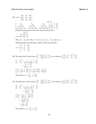
![SSM: Elementary Linear Algebra Section 1.4
17
(l) False; for example, if
1 2
3 4
,
A
⎡ ⎤
= ⎢ ⎥
⎣ ⎦
1 5
3 7
,
B
⎡ ⎤
= ⎢ ⎥
⎣ ⎦
and
1 0
0 0
,
C
⎡ ⎤
= ⎢ ⎥
⎣ ⎦
then
1 0
3 0
.
AC BC
⎡ ⎤
= = ⎢ ⎥
⎣ ⎦
(m) True; if A is an m × n matrix, then for both AB
and BA to be defined B must be an n × m matrix.
Then AB will be an m × m matrix and BA will be
an n × n matrix, so m = n in order for the sum to
be defined.
(n) True; since the jth column vector of AB is
A[jth column vector of B], a column of zeros in
B will result in a column of zeros in AB.
(o) False;
1 0 1 5 1 5
0 0 3 7 0 0
⎡ ⎤ ⎡ ⎤ ⎡ ⎤
=
⎢ ⎥ ⎢ ⎥ ⎢ ⎥
⎣ ⎦ ⎣ ⎦ ⎣ ⎦
Section 1.4
Exercise Set 1.4
5. 1
3
1
5 20
1 1
5 10
1 4 3
4 2
2 4 3 4
1 4 3
4 2
20
( )
B− ⎡ ⎤
= ⎢ ⎥
−
⋅ − − ⎣ ⎦
⎡ ⎤
= ⎢ ⎥
−
⎣ ⎦
⎡ ⎤
=
⎢ ⎥
−
⎢ ⎥
⎣ ⎦
7.
1
1 2
1
3
0
1 1
3 0 3 0
0 2 0 2
2 3 0 6 0
D−
⎡ ⎤
⎡ ⎤ ⎡ ⎤ ⎢ ⎥
= = =
⎢ ⎥ ⎢ ⎥
⋅ − ⎣ ⎦ ⎣ ⎦ ⎢ ⎥
⎣ ⎦
9. Here,
1
2
( )
x x
a d e e−
= = + and
1
2
( ),
x x
b c e e−
= = − so
2 2
2 2 2 2
1 1
4 4
1 1
2 2
4 4
1
( ) ( )
( ) ( )
.
x x x x
x x x x
ad bc e e e e
e e e e
− −
− −
− = + − −
= + + − − +
=
Thus,
1
1 1
2 2
1 1
2 2
1 1
2 2
1 1
2 2
( ) ( )
( ) ( )
( ) ( )
.
( ) ( )
x x x x
x x x x
x x x x
x x x x
e e e e
e e e e
e e e e
e e e e
−
− −
− −
− −
− −
⎡ ⎤
+ −
⎢ ⎥
⎢ ⎥
− +
⎣ ⎦
⎡ ⎤
+ − −
⎢ ⎥
=
⎢ ⎥
− − +
⎣ ⎦
11.
2 4
3 4
;
T
B
⎡ ⎤
= ⎢ ⎥
−
⎣ ⎦
1 1
1 1
5 5
3 1
20 10
1 4 4
3 2
8 12
( ) ( )
T T
B B
− −
⎡ ⎤
−
−
⎡ ⎤ ⎢ ⎥
= = =
⎢ ⎥
+ ⎣ ⎦ ⎢ ⎥
⎣ ⎦
13.
70 45
122 79
ABC
⎡ ⎤
= ⎢ ⎥
⎣ ⎦
1 1 79 45
122 70
70 79 122 45
1 79 45
122 70
40
( )
ABC − −
⎡ ⎤
= ⎢ ⎥
−
⋅ − ⋅ ⎣ ⎦
−
⎡ ⎤
= ⎢ ⎥
−
⎣ ⎦
1 1 1
1 4 1 4
2 6 2 6
6 1 4 2 2
( ) ( )
C− − − − −
⎡ ⎤ ⎡ ⎤
= =
⎢ ⎥ ⎢ ⎥
− − − ⎣ ⎦ ⎣ ⎦
1 1 1
4 3 4 3
4 2 4 2
2 4 3 4 20
( )
B− ⎡ ⎤ ⎡ ⎤
= =
⎢ ⎥ ⎢ ⎥
− −
⋅ − − ⎣ ⎦ ⎣ ⎦
1 1 2 1 2 1
5 3 5 3
3 2 1 5
A− − −
⎡ ⎤ ⎡ ⎤
= =
⎢ ⎥ ⎢ ⎥
− −
⋅ − ⋅ ⎣ ⎦ ⎣ ⎦
1 1 1 1 1 4 4 3 2 1
2 6 4 2 5 3
40
1 79 45
122 70
40
C B A
− − − ⎛ ⎞
− − −
⎡ ⎤ ⎡ ⎤ ⎡ ⎤
= ⎜ ⎟
⎢ ⎥ ⎢ ⎥ ⎢ ⎥
− −
⎣ ⎦ ⎣ ⎦ ⎣ ⎦
⎝ ⎠
−
⎡ ⎤
= ⎢ ⎥
−
⎣ ⎦
15. 1 1
7 7
1 2 7
1 3
3 2 1 7
2 7
1
1 3
2 7
1 3
(( ) )
( )( )
A A − −
=
− −
⎡ ⎤
= ⎢ ⎥
− −
− − − ⋅ ⎣ ⎦
− −
⎡ ⎤
= − ⎢ ⎥
− −
⎣ ⎦
⎡ ⎤
= ⎢ ⎥
⎣ ⎦
Thus
2
7
3
1
7 7
1
.
A
⎡ ⎤
⎢ ⎥
=
⎢ ⎥
⎣ ⎦
17. 1 1
5 2
13 13
4 1
13 13
2 2
1 5 2
4 1
1 5 2 4
1 5 2
4 1
13
(( ) )
I A I A − −
+ = +
−
⎡ ⎤
= ⎢ ⎥
− −
− ⋅ − ⋅ ⎣ ⎦
−
⎡ ⎤
= − ⎢ ⎥
− −
⎣ ⎦
⎡ ⎤
−
⎢ ⎥
=
⎢ ⎥
⎣ ⎦](https://image.slidesharecdn.com/elementary-linear-algebra-chapter1-220420115526/85/Elementary-linear-algebra-chapter-1-pdf-17-320.jpg)
![SSM: Elementary Linear Algebra Section 10.4
219
3 2 3 2
2
2
000088
6
( ) ( )
. ,
y y M M h
c
h
− +
= − = 4 3 4 3
3
2
000092
6
( ) ( )
. ,
y y M M h
c
h
− +
= − = −
5 4 5 4
4
2
000212
6
( ) ( )
. ,
y y M M h
c
h
− +
= − = −
1 1 99815
. ,
d y
= = 2 2 99987
. ,
d y
= = 3 3 99973
. ,
d y
= = 4 4 99823
. .
d y
= =
The resulting natural spline is
3
3 2
3 2
3 2
00000042 10 000214 10 99815 10 0
00000024 0000126 000088 99987 0 10
00000004 10 0000054 10 000092 10 99973 10 20
00000022 20 0000066 20 0
. ( ) . ( ) . ,
. ( ) . ( ) . ( ) . ,
( )
. ( ) . ( ) . ( ) . ,
. ( ) . ( ) .
x x x
x x x x
S x
x x x x
x x
− + + + + − ≤ ≤
− + + ≤ ≤
=
− − − − − − + ≤ ≤
− − − − − 00212 20 99823 20 30
( ) . , .
x x
⎧
⎪
⎪
⎨
⎪
⎪ − + ≤ ≤
⎩
Assuming the maximum is attained in the interval [0, 10] we set ( )
S x
′ equal to zero in this interval:
2
00000072 0000252 000088 0
( ) . . . .
S x x x
′ = − + =
To three significant digits the root of this quadratic equation in the interval [0, 10] is x = 3.93, and
S(3.93) = 1.00004.
5. The linear system (24) for the cubic runout spline becomes
2
3
4
6 0 0 0001116
1 4 1 0000816
0 0 6 0000636
.
.
.
.
M
M
M
⎡ ⎤ −
⎡ ⎤ ⎡ ⎤
⎢ ⎥
⎢ ⎥ ⎢ ⎥
= −
⎢ ⎥
⎢ ⎥ ⎢ ⎥
−
⎣ ⎦ ⎣ ⎦
⎣ ⎦
Solving this system yields 2 0000186
. ,
M = − 3 0000131
. ,
M = − 4 0000106
. .
M = −
From (22) and (23) we have 1 2 3
2 0000241
. ,
M M M
= − = − 5 4 3
2 0000081
. .
M M M
= − = −
Solving for the ai’s, bi’s, ci’s, and di’s from Equations (14) we have 2 1
1 00000009
6
( )
. ,
M M
a
h
−
= =
3 2
2 00000009
6
( )
. ,
M M
a
h
−
= = 4 3
3 00000004
6
( )
. ,
M M
a
h
−
= = 5 4
4 00000004
6
( )
. .
M M
a
h
−
= =
1
1 0000121
2
. ,
M
b = = − 2
2 0000093
2
. ,
M
b = = − 3
3 0000066
2
. ,
M
b = = − 4
4 0000053
2
. ,
M
b = = −
2 1 2 1
1
2
000282
6
( ) ( )
. ,
y y M M h
c
h
− +
= − = 3 2 3 2
2
2
000070
6
( ) ( )
. ,
y y M M h
c
h
− +
= − =
4 3 4 3
3
2
000087
6
( ) ( )
. ,
y y M M h
c
h
− +
= − = − 5 4 5 4
4
2
000207
6
( ) ( )
. ,
y y M M h
c
h
− +
= − = −
1 1 99815
. ,
d y
= = 2 2 99987
. ,
d y
= = 3 3 99973
. ,
d y
= = 4 4 99823
. .
d y
= =
The resulting cubic runout spline is
3 2
3 2
3 2
3
00000009 10 0000121 10 000282 10 99815 10 0
00000009 0000093 000070 99987 0 10
00000004 10 0000066 10 000087 10 99973 10 20
00000004 20 0000
. ( ) . ( ) . ( ) . ,
. ( ) . ( ) . ( ) . ,
( )
. ( ) . ( ) . ( ) . ,
. ( ) .
x x x x
x x x x
S x
x x x x
x
+ − + + + + − ≤ ≤
− + + ≤ ≤
=
− − − − − + ≤ ≤
− − 2
053 20 000207 20 99823 20 30
( ) . ( ) . , .
x x x
⎧
⎪
⎪
⎨
⎪
⎪ − − − + ≤ ≤
⎩
Assuming the maximum is attained in the interval [0, 10], we set ( )
S x
′ equal to zero in this interval:
2
00000027 0000186 000070 0
( ) . . . .
S x x x
′ = − + =
To three significant digits the root of this quadratic equation in the interval [0, 10] is 4.00 and S(4.00) = 1.00001.](https://image.slidesharecdn.com/elementary-linear-algebra-chapter1-220420115526/85/Elementary-linear-algebra-chapter-1-pdf-52-320.jpg)
![SSM: Elementary Linear Algebra Section 10.6
223
7. Let 1 2
[ ]T
x x
=
x be the state vector, with
1 probability
x = that John is happy and
2 probability
x = that John is sad. The transition
matrix P will be
4 2
5 3
1 1
5 3
P
⎡ ⎤
⎢ ⎥
=
⎢ ⎥
⎣ ⎦
since the columns
must sum to one. We find the steady state vector
for P by solving
1 2
5 3 1
1 2
2
5 3
0
0
,
q
q
⎡ ⎤
− ⎡ ⎤ ⎡ ⎤
⎢ ⎥ =
⎢ ⎥ ⎢ ⎥
− ⎣ ⎦
⎢ ⎥ ⎣ ⎦
⎣ ⎦
i.e.,
1 2
1 2
5 3
,
q q
= so
10
3
1
.
s
⎡ ⎤
= ⎢ ⎥
⎢ ⎥
⎣ ⎦
q Let
3
13
s = and get
10
13
3
13
,
⎡ ⎤
⎢ ⎥
=
⎢ ⎥
⎣ ⎦
q so
10
13
is the probability that John will
be happy on a given day.
8. The state vector 1 2 3
[ ]T
x x x
=
x will
represent the proportion of the population living
in regions 1, 2, and 3, respectively. In the
transition matrix, ij
p will represent the
proportion of the people in region j who move to
region i, yielding
90 15 10
05 75 05
05 10 85
. . .
.
. . .
. . .
P
⎡ ⎤
⎢ ⎥
=
⎢ ⎥
⎣ ⎦
1
2
3
10 15 10 0
05 25 05 0
05 10 15 0
. . .
. . .
. . .
q
q
q
⎡ ⎤
− −
⎡ ⎤ ⎡ ⎤
⎢ ⎥
⎢ ⎥ ⎢ ⎥
=
− −
⎢ ⎥
⎢ ⎥ ⎢ ⎥
− −
⎣ ⎦ ⎣ ⎦
⎣ ⎦
First reduce to row echelon form
13
7
4
7
1 0
0 1
0 0 0
,
⎡ ⎤
−
⎢ ⎥
−
⎢ ⎥
⎢ ⎥
⎣ ⎦
yielding
13
7
4
7
1
.
s
⎡ ⎤
⎢ ⎥
= ⎢ ⎥
⎢ ⎥
⎣ ⎦
q Set
7
24
s = and get
13
24
4
24
7
24
,
q
⎡ ⎤
⎢ ⎥
= ⎢ ⎥
⎢ ⎥
⎢ ⎥
⎣ ⎦
i.e., in the long run
13
24
1
or 54
6
%
⎛ ⎞
⎜ ⎟
⎝ ⎠
of the people reside in region 1,
4 2
or 16
24 3
%
⎛ ⎞
⎜ ⎟
⎝ ⎠
in region 2, and
7 1
or 29
24 6
%
⎛ ⎞
⎜ ⎟
⎝ ⎠
in region 3.
Section 10.6
Exercise Set 10.6
1. Note that the matrix has the same number of
rows and columns as the graph has vertices, and
that ones in the matrix correspond to arrows in
the graph.
(a)
0 0 0 1
1 0 1 1
1 1 0 1
0 0 0 0
⎡ ⎤
⎢ ⎥
⎢ ⎥
⎢ ⎥
⎢ ⎥
⎣ ⎦
(b)
0 1 1 0 0
0 0 0 0 1
1 0 0 1 0
0 0 1 0 0
0 0 1 0 0
⎡ ⎤
⎢ ⎥
⎢ ⎥
⎢ ⎥
⎢ ⎥
⎢ ⎥
⎣ ⎦
(c)
0 1 0 1 0 0
1 0 0 0 0 0
0 1 0 1 1 1
0 0 0 0 0 1
0 0 0 0 0 1
0 0 1 0 1 0
⎡ ⎤
⎢ ⎥
⎢ ⎥
⎢ ⎥
⎢ ⎥
⎢ ⎥
⎢ ⎥
⎣ ⎦
2. See the remark in problem 1; we obtain
(a) P
1 P
2
P
3
P
4
(b)
P
1
P
4
P3
P
5
P2](https://image.slidesharecdn.com/elementary-linear-algebra-chapter1-220420115526/85/Elementary-linear-algebra-chapter-1-pdf-56-320.jpg)
![Chapter 10: Applications of Linear Algebra SSM: Elementary Linear Algebra
226
(b) If player R uses strategy 1 2 3
[ ]
p p p
against player C’s strategy
1
4
1
4
1
4
1
4
⎡ ⎤
⎢ ⎥
⎢ ⎥
⎢ ⎥
⎢ ⎥
⎢ ⎥
⎢ ⎥
⎣ ⎦
his payoff
will be 1 2 3
1 9
4 4
.
A
⎛ ⎞ ⎛ ⎞
= + −
−
⎜ ⎟ ⎜ ⎟
⎝ ⎠ ⎝ ⎠
p q p p p Since
1,
p 2,
p and 3
p are nonnegative and add
up to 1, this is a weighted average of the
numbers
1
4
,
−
9
4
, and −1. Clearly this is the
largest if 1 3 0
p p
= = and 2 1;
p = that is,
0 1 0
[ ].
=
p
(c) As in (b), if player C uses
1 2 3 4
[ ]T
q q q q against 1 1
2 2
0 ,
⎡ ⎤
⎣ ⎦
we get 1 2 3 4
1
6 3
2
.
A q q q q
= − + + −
p q
Clearly this is minimized over all strategies
by setting 1 1
q = and 2 3 4 0.
q q q
= = =
That is 1 0 0 0
[ ] .
T
=
q
2. As per the hint, we will construct a 3 × 3 matrix
with two saddle points, say 11 33 1.
a a
= = Such a
matrix is
1 2 1
0 7 0
1 2 1
.
A
⎡ ⎤
⎢ ⎥
=
⎢ ⎥
⎣ ⎦
Note that
13 31 1
a a
= = are also saddle points.
3. (a) Calling the matrix A, we see 22
a is a saddle
point, so the optimal strategies are pure,
namely: 0 1
* [ ],
=
p
0
1
* ,
⎡ ⎤
= ⎢ ⎥
⎣ ⎦
q the value of
the game is 22 3.
v a
= =
(b) As in (a), 21
a is a saddle point, so optimal
strategies are 0 1 0
* [ ],
=
p
1
0
* ,
⎡ ⎤
= ⎢ ⎥
⎣ ⎦
q the
value of the game is 21 2.
v a
= =
(c) Here, 32
a is a saddle point, so optimal
strategies are 0 0 1
* [ ],
=
p
0
1
0
*
⎡ ⎤
⎢ ⎥
=
⎢ ⎥
⎣ ⎦
q and
32 2.
v a
= =
(d) Here, 21
a is a saddle point, so
0 1 0 0
* [ ],
=
p
1
0
0
*
⎡ ⎤
⎢ ⎥
=
⎢ ⎥
⎣ ⎦
q and
21 2.
v a
= = −
4. (a) Calling the matrix A, the formulas of
Theorem 10.7.2 yield 5 3
8 8
* ,
⎡ ⎤
=
⎣ ⎦
p
1
8
7
8
* ,
⎡ ⎤
⎢ ⎥
=
⎢ ⎥
⎣ ⎦
q
27
8
v = (A has no saddle points).
(b) As in (a), 40 20 2 1
3 3
60 60
* ,
⎡ ⎤ ⎡ ⎤
= =
⎣ ⎦
⎣ ⎦
p
10 1
6
60
5
50
6
60
* ,
⎡ ⎤ ⎡ ⎤
⎢ ⎥ ⎢ ⎥
= =
⎢ ⎥ ⎢ ⎥
⎣ ⎦
⎣ ⎦
q
1400 70
60 3
v = = (Again, A
has no saddle points).
(c) For this matrix, 11
a is a saddle point, so
1 0
* [ ],
=
p
1
0
* ,
⎡ ⎤
= ⎢ ⎥
⎣ ⎦
q and 11 3.
v a
= =
(d) This matrix has no saddle points, so, as in
(a), 3 3
2 2
5 5 5 5
* ,
− −
− −
⎡ ⎤ ⎡ ⎤
= =
⎣ ⎦ ⎣ ⎦
p
3 3
5 5
2 2
5 5
* ,
−
−
−
−
⎡ ⎤ ⎡ ⎤
⎢ ⎥ ⎢ ⎥
= =
⎢ ⎥ ⎢ ⎥
⎣ ⎦ ⎣ ⎦
q and
19 19
5 5
.
v
−
= =
−
(e) Again, A has no saddle points, so as in (a),
3 10
13 13
* ,
⎡ ⎤
=
⎣ ⎦
p
1
13
12
13
* ,
⎡ ⎤
⎢ ⎥
=
⎢ ⎥
⎣ ⎦
q and
29
13
.
v
−
=
5. Let
11 payoff
a = to R if the black ace and black two
are played = 3.
12 payoff
a = to R if the black ace and red three
are played = −4.
21 payoff
a = to R if the red four and black two
are played = −6.
22 payoff
a = to R if the red four and red three](https://image.slidesharecdn.com/elementary-linear-algebra-chapter1-220420115526/85/Elementary-linear-algebra-chapter-1-pdf-59-320.jpg)
![Chapter 10: Applications of Linear Algebra SSM: Elementary Linear Algebra
228
120
100
106 67
;
.
⎡ ⎤
⎢ ⎥
=
⎢ ⎥
⎣ ⎦
p i.e., the price of tomatoes was
$120, corn was $100, and lettuce was $106.67.
5. Taking the CE, EE, and ME in that order, we
form the consumption matrix C, where the
ij
c =
amount (per consulting dollar) of the i-th
engineer’s services purchased by the j-th
engineer. Thus,
0 2 3
1 0 4
3 4 0
. .
.
. .
. .
C
⎡ ⎤
⎢ ⎥
=
⎢ ⎥
⎣ ⎦
We want to solve (I − C)x = d, where d is the
demand vector, i.e.
1
2
3
1 2 3 500
1 1 4 700
3 4 1 600
. .
.
. .
. .
x
x
x
⎡ ⎤
− −
⎡ ⎤ ⎡ ⎤
⎢ ⎥
⎢ ⎥ ⎢ ⎥
=
− −
⎢ ⎥
⎢ ⎥ ⎢ ⎥
− −
⎣ ⎦ ⎣ ⎦
⎣ ⎦
In row-echelon form this reduces to
1
2
3
1 2 3 500
0 1 43877 765 31
0 0 1 1556 19
. .
.
. .
.
x
x
x
⎡ ⎤
− −
⎡ ⎤ ⎡ ⎤
⎢ ⎥
⎢ ⎥ ⎢ ⎥
=
−
⎢ ⎥
⎢ ⎥ ⎢ ⎥
⎣ ⎦ ⎣ ⎦
⎣ ⎦
Back-substitution yields the solution
1256 48
1448 12
1556 19
.
.
.
.
⎡ ⎤
⎢ ⎥
=
⎢ ⎥
⎣ ⎦
x
The CE received $1256, the EE received $1448,
and the ME received $1556.
6. (a) The solution of the system (I − C)x = d is
1
( ) .
I C −
= −
x d The effect of increasing the
demand i
d for the ith industry by one unit
is the same as adding
0
0
1
0
0
⎡ ⎤
⎢ ⎥
⎢ ⎥
⎢ ⎥
⎢ ⎥
⎢ ⎥
⎢ ⎥
⎢ ⎥
⎢ ⎥
⎣ ⎦
#
#
to d where the 1
is in the ith row. The new solution is
1 1
0 0
0 0
1 1
0 0
0 0
( ) ( )
I C I C
− −
⎛ ⎞
⎡ ⎤ ⎡ ⎤
⎜ ⎟
⎢ ⎥ ⎢ ⎥
⎜ ⎟
⎢ ⎥ ⎢ ⎥
⎜ ⎟
⎢ ⎥ ⎢ ⎥
− + = + −
⎜ ⎟
⎢ ⎥ ⎢ ⎥
⎜ ⎟
⎢ ⎥ ⎢ ⎥
⎜ ⎟
⎢ ⎥ ⎢ ⎥
⎜ ⎟
⎢ ⎥ ⎢ ⎥
⎜ ⎟
⎢ ⎥ ⎢ ⎥
⎣ ⎦ ⎣ ⎦
⎝ ⎠
d x
# #
# #
which has the effect of adding the ith
column of 1
( )
I C −
− to the original solution.
(b) The increase in value is the second column
of 1
( ) ,
I C −
−
542
1
690
503 170
.
⎡ ⎤
⎢ ⎥
⎢ ⎥
⎣ ⎦
Thus the value of
the coal-mining operation must increase by
542
503
.
7. The i-th column sum of E is
1
,
n
ji
j
e
=
∑ and the
elements of the i-th column of I − E are the
negatives of the elements of E, except for the
ii-th, which is 1 .
ii
e
− So, the i-th column sum of
I − E is
1
1 1 1 0.
n
ji
j
e
=
− = − =
∑ Now, ( )T
I E
− has
zero row sums, so the vector 1 1 1
[ ]T
=
x "
solves 0
( ) .
T
I E
− =
x This implies
0
det( ) .
T
I E
− = But det( ) det( ),
T
I E I E
− = −
so (I − E)p = 0 must have nontrivial (i.e.,
nonzero) solutions.
The CE received $1256, the EE received $1448,
and the ME received $1556.
8. Let C be a consumption matrix whose column
sums are less than one; then the row sums of T
C
are less than one. By Corollary 10.8.4, T
C is
productive so 1
0
( ) .
T
I C −
− ≥ But
1 1
1
0
( ) ((( ) )) )
(( ) )
.
T T
T T
I C I C
I C
− −
−
− = −
= −
≥
Thus, C is productive.
Section 10.9
Exercise Set 10.9
1. Using Equation (18), we calculate
2
3 3
2
30
15
2
50 100
7
2
.
s
Yld s
s s
Yld
= =
= =
+
So all the trees in the second class should be
harvested for an optimal yield (since s = 1000)
of $15,000.](https://image.slidesharecdn.com/elementary-linear-algebra-chapter1-220420115526/85/Elementary-linear-algebra-chapter-1-pdf-61-320.jpg)
![SSM: Elementary Linear Algebra Section 10.12
233
(c) 1 0
1 1
4 4
1 1 1
4 4 2
1 1
4 4 1
1 1 2
4 4
1
2
1
2
0 0 0
0
0 0 0
0 0
0 0
0
0 0
0
0
( ) ( )
M
= +
⎡ ⎤ ⎡ ⎤
⎢ ⎥ ⎡ ⎤ ⎢ ⎥
⎢ ⎥ ⎢ ⎥ ⎢ ⎥
= +
⎢ ⎥ ⎢ ⎥ ⎢ ⎥
⎢ ⎥ ⎢ ⎥ ⎢ ⎥
⎢ ⎥
⎢ ⎥ ⎣ ⎦ ⎢ ⎥
⎣ ⎦
⎢ ⎥
⎣ ⎦
⎡ ⎤
⎢ ⎥
⎢ ⎥
=
⎢ ⎥
⎢ ⎥
⎢ ⎥
⎣ ⎦
t t b
1
8
5
2 1 8
1
8
5
8
( ) ( )
,
M
⎡ ⎤
⎢ ⎥
⎢ ⎥
= + = ⎢ ⎥
⎢ ⎥
⎢ ⎥
⎢ ⎥
⎣ ⎦
t t b
3
16
11
3 2 16
3
16
11
16
( ) ( )
M
⎡ ⎤
⎢ ⎥
⎢ ⎥
= + = ⎢ ⎥
⎢ ⎥
⎢ ⎥
⎢ ⎥
⎣ ⎦
t t b
7
32
23
4 3 32
7
32
23
32
( ) ( )
,
M
⎡ ⎤
⎢ ⎥
⎢ ⎥
= + = ⎢ ⎥
⎢ ⎥
⎢ ⎥
⎢ ⎥
⎣ ⎦
t t b
15
64
47
5 4 64
15
64
47
64
( ) ( )
M
⎡ ⎤
⎢ ⎥
⎢ ⎥
= + = ⎢ ⎥
⎢ ⎥
⎢ ⎥
⎢ ⎥
⎣ ⎦
t t b
15 1
1
64 64
4
47 3 1
5 64 64
4
15 1 1
4 64
64
3 1
47
4 64
64
( )
⎡ ⎤ ⎡ ⎤
⎡ ⎤ −
⎢ ⎥ ⎢ ⎥
⎢ ⎥
⎢ ⎥ −
⎢ ⎥
⎢ ⎥
− = − =
⎢ ⎥ ⎢ ⎥
⎢ ⎥
−
⎢ ⎥ ⎢ ⎥
⎢ ⎥
⎢ ⎥ ⎢ ⎥
⎢ ⎥
−
⎢ ⎥ ⎢ ⎥ ⎢ ⎥
⎣ ⎦ ⎣ ⎦
⎣ ⎦
t t
(d) Using
percentage error
computed value actual value
100
actual value
%
−
= ×
we have that the percentage error for 1
t and
3
t was
0371
100 12 9
2871
.
% . %,
.
−
× = − and for
2
t and 4
t was
0371
100 5 2
7129
.
% . %.
.
× =
2. The average value of the temperature on the
circle is
1
2
( ) ,
f r d
r
π
π
θ θ
π −
∫ where r is the radius
of the circle and f(θ) is the temperature at the
point of the circumference where the radius to
that point makes the angle θ with the horizontal.
Clearly f(θ) = 1 for
2 2
π π
θ
−
< < and is zero
otherwise. Consequently, the value of the
integral above (which equals the temperature at
the center of the circle) is
1
2
.
3. As in 1(c), but using M and b as in the problem
statement, we obtain
1 0
3 5 5 5 3
1 1
4 4 2 4 2 4 4
1 1
( ) ( )
T
M
= +
⎡ ⎤
= ⎣ ⎦
t t b
2 1
13 9 9 13 7 15
11 21
16 8 16 8 16 16 16 8
1
( ) ( )
.
T
M
= +
⎡ ⎤
=
⎣ ⎦
t t b
Section 10.12
Exercise Set 10.12
1. (c) The linear system
31 31 32
1
28
20
* * *
[ ]
x x x
= + −
32 31 32
1
24 3 3
20
* * *
[ ]
x x x
= + −
can be rewritten as
31 32
31 32
19 28
3 23 24
* *
* *
,
x x
x x
+ =
− + =
which has the solution
31
32
31
22
27
22
*
*
.
x
x
=
=
2. (a) Setting
( ) ( )
1 1 1 0 0
0 01 02 31 32
0 0
( ) ( ) ( ) ( ) ( ) ( , ),
, ,
x x x x
= = =
x and
using part (b) of Exercise 1, we have](https://image.slidesharecdn.com/elementary-linear-algebra-chapter1-220420115526/85/Elementary-linear-algebra-chapter-1-pdf-66-320.jpg)
![Chapter 10: Applications of Linear Algebra SSM: Elementary Linear Algebra
234
1
31
1
28 1 40000
20
( )
[ ] .
x = =
1
32
1
24 1 20000
20
( )
[ ] .
x = =
2
31
1
28 1 4 1 2 1 41000
20
( )
[ . . ] .
x = + − =
2
32
1
24 3 1 4 3 1 2 1 23000
20
( )
[ ( . ) ( . )] .
x = + − =
3
31
1
28 1 41 1 23 1 40900
20
( )
[ . . ] .
x = + − =
3
32
1
24 3 1 41 3 1 23 1 22700
20
( )
[ ( . ) ( . )] .
x = + − =
4
31
1
28 1 409 1 227 1 40910
20
( )
[ . . ] .
x = + − =
4
32
1
24 3 1 409 3 1 227
20
1 22730
( )
[ ( . ) ( . )]
.
x = + −
=
5
31
1
28 1 4091 1 2273 1 40909
20
( )
[ . . ] .
x = + − =
5
32
1
24 3 1 4091 3 1 2273
20
1 22727
( )
[ ( . ) ( . )]
.
x = + −
=
6
31
1
28 1 40909 1 22727
20
1 40909
( )
[ . . ]
.
x = + −
=
6
32
1
24 3 1 40909 3 1 22727
20
1 22727
( )
[ ( . ) ( . )]
. .
x = + −
=
(b) ( )
1 0 0
0 31 32
1 1
( ) ( ) ( )
( , ) ,
x x
= =
x
1
31
1
28 1 1 1 4
20
( )
[ ] .
x = + − =
2
32
1
24 3 1 3 1 1 2
20
( )
[ ( ) ( )] .
x = + − =
Since 1
3
( )
x in this part is the same as 1
3
( )
x in part (a), we will get 2
3
( )
x as in part (a) and therefore 3 6
3 3
( ) ( )
, ...,
x x
will also be the same as in part (a).
(c) ( )
1 0 0
0 31 32
148 15
( ) ( ) ( )
( , ) ,
x x
= − =
x
1
31
1
28 148 15 9 55000
20
( )
[ ( )] .
x = + − − =
1
32
1
24 3 148 3 15 25 65000
20
( )
[ ( ) ( )] .
x = + − − =
2
31
1
28 9 55 25 65 0 59500
20
( )
[ . . ] .
x = + − =](https://image.slidesharecdn.com/elementary-linear-algebra-chapter1-220420115526/85/Elementary-linear-algebra-chapter-1-pdf-67-320.jpg)
![SSM: Elementary Linear Algebra Section 10.12
235
2
32
1
24 3 9 55 3 25 65
20
1 21500
( )
[ ( . ) ( . )]
.
x = + −
= −
3
31
1
28 0 595 1 215
20
1 49050
( )
[ . . ]
.
x = + +
=
3
32
1
24 3 0 595 3 1 215
20
1 47150
( )
[ ( . ) ( . )]
.
x = + +
=
4
31
1
28 1 4905 1 4715 1 40095
20
( )
[ . . ] .
x = + − =
4
32
1
24 3 1 4905 3 1 4715
20
1 20285
( )
[ ( . ) ( . )]
.
x = + −
=
5
31
1
28 1 40095 1 20285
20
1 40991
( )
[ . . ]
.
x = + −
=
5
32
1
24 3 1 40095 3 1 20285
20
1 22972
( )
[ ( . ) ( . )]
.
x = + −
=
6
31
1
28 1 40991 1 22972 1 40901
20
( )
[ . . ] .
x = + − =
6
32
1
24 3 1 40991 3 1 22972
20
1 22703
( )
[ ( . ) ( . )]
.
x = + −
=
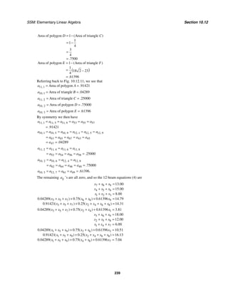
4. Referring to the figure below and starting with 1
0 0 0
( )
( , ) :
=
x
1
0
( )
x is projected to 1
1
( )
x on 1,
L 1
1
( )
x is projected to 1
2
( )
x on 2,
L 1
2
( )
x is projected to 1
3
( )
x on 3,
L and so on.
L1 x1 x1
x2
x0
x3
A
B
x2
x2 = 1
x1 – x2 = 0 x1 – x2 = 2
x1
L3
L2
(1)
(1)
(1)
(1)
(2)
As seen from the graph the points of the limit cycle are 1 ,
∗
=
x A 2 ,
∗
=
x B 3 .
∗
=
x A
Since 1
∗
x is the point of intersection of 1
L and 3
L it follows on solving the system
12
11 12
1
0
*
x
x x
∗
∗
=
− =
that 1 1 1
*
( , ).
=
x Since 2 21 22
( , )
x x
∗ ∗ ∗
=
x is on 2,
L it follows that 21 22 2.
x x
∗ ∗
− = Now 1 2
∗ ∗
x x is perpendicular to 2,
L](https://image.slidesharecdn.com/elementary-linear-algebra-chapter1-220420115526/85/Elementary-linear-algebra-chapter-1-pdf-68-320.jpg)
![Chapter 10: Elementary Linear Algebra SSM: Elementary Linear Algebra
250
1
2
,
x ≠ otherwise we obtain the 2-cycle
1 1
2 2
1
2
0
0 0
.
⎡ ⎤ ⎡ ⎤ ⎡ ⎤
→ →
⎢ ⎥ ⎢ ⎥ ⎢ ⎥
⎣ ⎦ ⎣ ⎦ ⎣ ⎦
Similarly, starting with a point of the form
0
y
⎡ ⎤
⎢ ⎥
⎣ ⎦
with 0 < y < 1, we obtain a 4-cycle
0 0 1 0
0 1 0
y y
y y y
−
⎡ ⎤ ⎡ ⎤ ⎡ ⎤ ⎡ ⎤ ⎡ ⎤
→ → → →
⎢ ⎥ ⎢ ⎥ ⎢ ⎥ ⎢ ⎥ ⎢ ⎥
−
⎣ ⎦ ⎣ ⎦ ⎣ ⎦ ⎣ ⎦ ⎣ ⎦
if
1
2
,
y ≠ otherwise we obtain the 2-cycle
1
2
1 1
2 2
0 0
0
.
⎡ ⎤ ⎡ ⎤ ⎡ ⎤
→ →
⎢ ⎥ ⎢ ⎥ ⎢ ⎥
⎣ ⎦ ⎣ ⎦ ⎣ ⎦
Thus every point not in
the interior of S is a periodic point with 1, 2,
or 4. Finally because no point in S can have
a dense set of iterates, it follows that the
mapping cannot be chaotic.
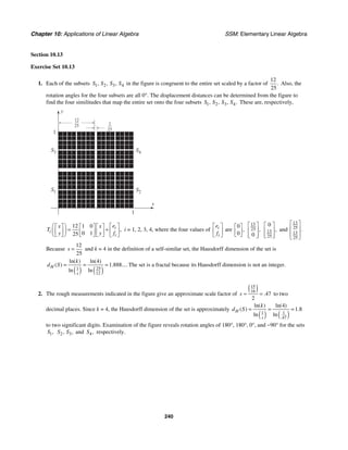
9. As per the hint, we wish to find the regions in S
that map onto the four indicated regions in the
figure below.
I'
II'
III'
IV'
(1, 1)
(0, 1)
(0, 0) (1, 0)
( , 0)
( , 1)
1
2
1
2
We first consider region ′
I with vertices (0, 0),
1
1
2
,
,
⎛ ⎞
⎜ ⎟
⎝ ⎠
and (1, 1). We seek points 1 1
( , ),
x y
2 2
( , ),
x y and 3 3
( , ),
x y with entries that lie in
[0, 1], that map onto these three points under the
mapping
1 1
1 2
x x a
y y b
⎡ ⎤ ⎡ ⎤ ⎡ ⎤ ⎡ ⎤
→ +
⎢ ⎥ ⎢ ⎥ ⎢ ⎥ ⎢ ⎥
⎣ ⎦ ⎣ ⎦ ⎣ ⎦ ⎣ ⎦
for certain
integer values of a and b to be determined. This
leads to the three equations
1
2
1
2 2
2
3
3
1 1 0
1 2 0
1 1
1 2 1
1 1 1
1 2 1
,
,
.
x a
y b
x a
y b
x a
y b
⎡ ⎤
⎡ ⎤ ⎡ ⎤ ⎡ ⎤
+ =
⎢ ⎥
⎢ ⎥ ⎢ ⎥ ⎢ ⎥
⎣ ⎦ ⎣ ⎦ ⎣ ⎦
⎣ ⎦
⎡ ⎤
⎡ ⎤
⎡ ⎤ ⎡ ⎤
+ = ⎢ ⎥
⎢ ⎥
⎢ ⎥ ⎢ ⎥
⎣ ⎦ ⎣ ⎦
⎣ ⎦ ⎣ ⎦
⎡ ⎤
⎡ ⎤ ⎡ ⎤ ⎡ ⎤
+ =
⎢ ⎥
⎢ ⎥ ⎢ ⎥ ⎢ ⎥
⎣ ⎦ ⎣ ⎦ ⎣ ⎦
⎣ ⎦
The inverse of the matrix
1 1
1 2
⎡ ⎤
⎢ ⎥
⎣ ⎦
is
2 1
1 1
.
−
⎡ ⎤
⎢ ⎥
−
⎣ ⎦
We multiply the above three matrix equations by
this inverse and set
2 1
1 1
.
c a
d b
−
⎡ ⎤ ⎡ ⎤ ⎡ ⎤
=
⎢ ⎥ ⎢ ⎥ ⎢ ⎥
−
⎣ ⎦ ⎣ ⎦ ⎣ ⎦
Notice
that c and d must be integers. This leads to
1
1
1
2 2
1
2 2
3
3
2 1 0
1 1 0
0
2 1
1 1 1
2 1 1 1
1 1 1 0
,
,
.
x c c
y d d
x c c
y d d
x c c
y d d
−
⎡ ⎤ ⎡ ⎤ ⎡ ⎤ ⎡ ⎤ ⎡ ⎤
= − = −
⎢ ⎥ ⎢ ⎥ ⎢ ⎥ ⎢ ⎥ ⎢ ⎥
−
⎣ ⎦ ⎣ ⎦ ⎣ ⎦ ⎣ ⎦
⎣ ⎦
⎡ ⎤ ⎡ ⎤
−
⎡ ⎤ ⎡ ⎤ ⎡ ⎤ ⎡ ⎤
= − = −
⎢ ⎥ ⎢ ⎥
⎢ ⎥ ⎢ ⎥ ⎢ ⎥ ⎢ ⎥
−
⎣ ⎦ ⎣ ⎦ ⎣ ⎦
⎣ ⎦ ⎣ ⎦ ⎣ ⎦
⎡ ⎤ −
⎡ ⎤ ⎡ ⎤ ⎡ ⎤ ⎡ ⎤ ⎡ ⎤
= − = −
⎢ ⎥ ⎢ ⎥ ⎢ ⎥ ⎢ ⎥ ⎢ ⎥ ⎢ ⎥
−
⎣ ⎦ ⎣ ⎦ ⎣ ⎦ ⎣ ⎦ ⎣ ⎦
⎣ ⎦
The only integer values of c and d that will give
values of i
x and i
y in the interval [0, 1] are
c = d = 0. This then gives a = b = 0 and the
mapping
1 1
1 2
x x
y y
⎡ ⎤ ⎡ ⎤ ⎡ ⎤
→
⎢ ⎥ ⎢ ⎥ ⎢ ⎥
⎣ ⎦ ⎣ ⎦ ⎣ ⎦
maps the three
points (0, 0),
1
0
2
,
,
⎛ ⎞
⎜ ⎟
⎝ ⎠
and (1, 0) to the three
points (0, 0),
1
1
2
,
,
⎛ ⎞
⎜ ⎟
⎝ ⎠
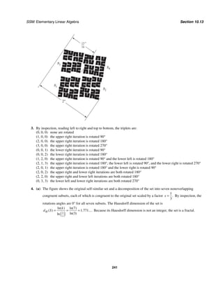
and (1, 1), respectively.
The three points (0, 0),
1
0
2
,
,
⎛ ⎞
⎜ ⎟
⎝ ⎠
and (1, 0) define
the triangular region labeled I in the diagram
below, which then maps onto the region .
′
I
I
II
III
IV
(1, 1)
(0, 1)
(0, 0) (1, 0)
(1, )
1
2
(0, )
1
2
For region ,
′
II the calculations are as follows:](https://image.slidesharecdn.com/elementary-linear-algebra-chapter1-220420115526/85/Elementary-linear-algebra-chapter-1-pdf-83-320.jpg)
![Chapter 10: Elementary Linear Algebra SSM: Elementary Linear Algebra
254
SL HK
19 12 8 11
so the corresponding plaintext and ciphertext
vectors are
1 1
1 19
18 12
⎡ ⎤ ⎡ ⎤
= ↔ =
⎢ ⎥ ⎢ ⎥
⎣ ⎦ ⎣ ⎦
p c
2 2
13 8
25 11
⎡ ⎤ ⎡ ⎤
= ↔ =
⎢ ⎥ ⎢ ⎥
⎣ ⎦ ⎣ ⎦
p c
We want to reduce 1
2
19 12
8 11
T
T
C
⎡ ⎤ ⎡ ⎤
= =
⎢ ⎥ ⎢ ⎥
⎣ ⎦
⎢ ⎥
⎣ ⎦
c
c
to I by
elementary row operations and simultaneously
apply these operations to 1
2
1 18
13 25
.
T
T
P
⎡ ⎤ ⎡ ⎤
= =
⎢ ⎥ ⎢ ⎥
⎣ ⎦
⎢ ⎥
⎣ ⎦
p
p
The calculations are as follows:
19 12 1 18
8 11 13 25
⎡ ⎤
⎢ ⎥
⎣ ⎦
Form the matrix
[ ].
C P
1 132 11 198
8 11 13 25
⎡ ⎤
⎢ ⎥
⎣ ⎦
Multiply the first row
by 1
19 11 (mod 26).
−
=
1 2 11 16
8 11 13 25
⎡ ⎤
⎢ ⎥
⎣ ⎦
Replace 132 and 198 by
their residues modulo
26.
1 2 11 16
0 5 75 103
⎡ ⎤
⎢ ⎥
− − −
⎣ ⎦
−8 times the first row to
the second.
1 2 11 16
0 21 3 1
⎡ ⎤
⎢ ⎥
⎣ ⎦
Replace the entries in
the second row by their
residues modulo 26.
1 2 11 16
0 1 15 5
⎡ ⎤
⎢ ⎥
⎣ ⎦
Multiply the second row
by 1
21 5 (mod 26).
−
=
1 0 19 6
0 1 15 5
−
⎡ ⎤
⎢ ⎥
⎣ ⎦
Add −2 times the
second row to the first.
1 0 7 6
0 1 15 5
⎡ ⎤
⎢ ⎥
⎣ ⎦
Replace −19 by its
residue modulo 26.
Thus 1 7 6
15 5
( )T
A− ⎡ ⎤
= ⎢ ⎥
⎣ ⎦
so the deciphering
matrix is 1 7 15
6 5
A− ⎡ ⎤
= ⎢ ⎥
⎣ ⎦
(mod 26).
Since 1
35 90 55 23(mod 26),
det( )
A−
= − = − =
1 1
1 5 15
23
6 7
5 15
17
6 7
85 255
102 119
7 5
(mod 26)
2 15
( )
A A− −
−
=
−
⎡ ⎤
= ⎢ ⎥
−
⎣ ⎦
−
⎡ ⎤
= ⎢ ⎥
−
⎣ ⎦
−
⎡ ⎤
= ⎢ ⎥
−
⎣ ⎦
⎡ ⎤
= ⎢ ⎥
⎣ ⎦
is the enciphering matrix.
5. From Table 1 the numerical equivalent of the
known plaintext is
AT OM
1 20 15 13
and the numerical equivalent of the
corresponding ciphertext is
JY QO
10 25 17 15
The corresponding plaintext and ciphertext
vectors are:
1 1
1 10
20 25
⎡ ⎤ ⎡ ⎤
= ↔ =
⎢ ⎥ ⎢ ⎥
⎣ ⎦ ⎣ ⎦
p c
2 2
15 17
13 15
⎡ ⎤ ⎡ ⎤
= ↔ =
⎢ ⎥ ⎢ ⎥
⎣ ⎦ ⎣ ⎦
p c
We want to reduce
10 25
17 15
C
⎡ ⎤
= ⎢ ⎥
⎣ ⎦
to I by
elementary row operations and simultaneously
apply these operations to
1 20
15 13
.
P
⎡ ⎤
= ⎢ ⎥
⎣ ⎦
The calculations are as follows:
10 25 1 20
17 15 15 13
⎡ ⎤
⎢ ⎥
⎣ ⎦
Form the matrix
[ ].
C P
27 40 16 33
17 15 15 13
⎡ ⎤
⎢ ⎥
⎣ ⎦
Add the second row to
the first (since 1
10−
does not exist mod 26).
1 14 16 7
17 15 15 13
⎡ ⎤
⎢ ⎥
⎣ ⎦
Replace the entries in
the first row by their
residues modulo 26.
1 14 16 7
0 223 257 106
⎡ ⎤
⎢ ⎥
− − −
⎣ ⎦
Add −17 times the first
row to the second.](https://image.slidesharecdn.com/elementary-linear-algebra-chapter1-220420115526/85/Elementary-linear-algebra-chapter-1-pdf-87-320.jpg)
![SSM: Elementary Linear Algebra Section 10.15
255
1 14 16 7
0 11 3 24
⎡ ⎤
⎢ ⎥
⎣ ⎦
Replace the entries in
the second row by their
residues modulo 26.
1 14 16 7
0 1 57 456
⎡ ⎤
⎢ ⎥
⎣ ⎦
Multiply the second row
by 1
11 19
−
= (mod 26).
1 14 16 7
0 1 5 14
⎡ ⎤
⎢ ⎥
⎣ ⎦
Replace the entries in
the second row by their
residues modulo 26.
1 0 54 189
0 1 5 14
− −
⎡ ⎤
⎢ ⎥
⎣ ⎦
Add −14 times the
second row to the first.
1 0 24 19
0 1 5 14
⎡ ⎤
⎢ ⎥
⎣ ⎦
Replace −54 and −189
by their residues
modulo 26.
Thus 1 24 19
5 14
( ) ,
T
A− ⎡ ⎤
= ⎢ ⎥
⎣ ⎦
and so the
deciphering matrix is 1 24 5
19 14
.
A− ⎡ ⎤
= ⎢ ⎥
⎣ ⎦
From Table 1 the numerical equivalent of the
given ciphertext is
LN GI HG YB VR EN JY
12 14 7 9 8 7 25 2 22 18 5 14 10 25
QO
17 15
To obtain the plaintext pairs, we multiply each
ciphertext vector by 1
:
A−
24 5 12 358 20
19 14 14 424 8
24 5 7 213 5
19 14 9 259 25
24 5 8 227 19
19 14 7 250 16
24 5 25 610 12
(mod 26)
19 14 2 503 9
24 5
T
H
E
Y
S
P
L
I
⎡ ⎤ ⎡ ⎤ ⎡ ⎤ ⎡ ⎤
= =
⎢ ⎥ ⎢ ⎥ ⎢ ⎥ ⎢ ⎥
⎣ ⎦ ⎣ ⎦ ⎣ ⎦ ⎣ ⎦
⎡ ⎤ ⎡ ⎤ ⎡ ⎤ ⎡ ⎤
= =
⎢ ⎥ ⎢ ⎥ ⎢ ⎥ ⎢ ⎥
⎣ ⎦ ⎣ ⎦ ⎣ ⎦ ⎣ ⎦
⎡ ⎤ ⎡ ⎤ ⎡ ⎤ ⎡ ⎤
= =
⎢ ⎥ ⎢ ⎥ ⎢ ⎥ ⎢ ⎥
⎣ ⎦ ⎣ ⎦ ⎣ ⎦ ⎣ ⎦
⎡ ⎤ ⎡ ⎤ ⎡ ⎤ ⎡ ⎤
= =
⎢ ⎥ ⎢ ⎥ ⎢ ⎥ ⎢ ⎥
⎣ ⎦ ⎣ ⎦ ⎣ ⎦ ⎣ ⎦
22 618 20
19 14 18 670 20
24 5 5 190 8
19 14 14 291 5
24 5 10 365 1
19 14 25 540 20
24 5 17 483 15
19 14 15 533 13
T
T
H
E
A
T
O
M
⎡ ⎤ ⎡ ⎤ ⎡ ⎤ ⎡ ⎤
= =
⎢ ⎥ ⎢ ⎥ ⎢ ⎥ ⎢ ⎥
⎣ ⎦ ⎣ ⎦ ⎣ ⎦ ⎣ ⎦
⎡ ⎤ ⎡ ⎤ ⎡ ⎤ ⎡ ⎤
= =
⎢ ⎥ ⎢ ⎥ ⎢ ⎥ ⎢ ⎥
⎣ ⎦ ⎣ ⎦ ⎣ ⎦ ⎣ ⎦
⎡ ⎤ ⎡ ⎤ ⎡ ⎤ ⎡ ⎤
= =
⎢ ⎥ ⎢ ⎥ ⎢ ⎥ ⎢ ⎥
⎣ ⎦ ⎣ ⎦ ⎣ ⎦ ⎣ ⎦
⎡ ⎤ ⎡ ⎤ ⎡ ⎤ ⎡ ⎤
= =
⎢ ⎥ ⎢ ⎥ ⎢ ⎥ ⎢ ⎥
⎣ ⎦ ⎣ ⎦ ⎣ ⎦ ⎣ ⎦
which yields the message THEY SPLIT THE
ATOM.
6. Since we want a Hill 3-cipher, we will group the
letters in triples. From Table 1 the numerical
equivalents of the known plaintext are
I H A V E C O M E
9 8 1 22 5 3 15 13 5
and the numerical equivalent of the
corresponding ciphertext are
H P A F Q G G D U
8 16 1 6 17 7 7 4 21
The corresponding plaintext and ciphertext
vectors are
1 1
9 8
8 16
1 1
⎡ ⎤ ⎡ ⎤
⎢ ⎥ ⎢ ⎥
= ↔ =
⎢ ⎥ ⎢ ⎥
⎣ ⎦ ⎣ ⎦
p c
2 2
22 6
5 17
3 7
⎡ ⎤ ⎡ ⎤
⎢ ⎥ ⎢ ⎥
= ↔ =
⎢ ⎥ ⎢ ⎥
⎣ ⎦ ⎣ ⎦
p c
3 3
15 7
13 4
5 21
⎡ ⎤ ⎡ ⎤
⎢ ⎥ ⎢ ⎥
= ↔ =
⎢ ⎥ ⎢ ⎥
⎣ ⎦ ⎣ ⎦
p c
We want to reduce
8 16 1
6 17 7
7 4 21
C
⎡ ⎤
⎢ ⎥
=
⎢ ⎥
⎣ ⎦
to I by
elementary row operations and simultaneously
apply these operations to
9 8 1
22 5 3
15 13 5
.
P
⎡ ⎤
⎢ ⎥
=
⎢ ⎥
⎣ ⎦
The calculations are as follows:
8 16 1 9 8 1
6 17 7 22 5 3
7 4 21 15 13 5
⎡ ⎤
⎢ ⎥
⎢ ⎥
⎣ ⎦
Form the matrix
[ ].
C P
15 20 22 24 21 6
6 17 7 22 5 3
7 4 21 15 13 5
⎡ ⎤
⎢ ⎥
⎢ ⎥
⎣ ⎦
Add the third row
to the first since 1
8−
does not exist modulo
26.
1 140 154 168 147 42
6 17 7 22 5 3
7 4 21 15 13 5
⎡ ⎤
⎢ ⎥
⎢ ⎥
⎣ ⎦
Multiply the first row
by 1
15 7
−
= (mod 26).](https://image.slidesharecdn.com/elementary-linear-algebra-chapter1-220420115526/85/Elementary-linear-algebra-chapter-1-pdf-88-320.jpg)
![SSM: Elementary Linear Algebra Section 10.16
257
7. (a) Multiply each of the triples of the message
by
1 1 0
0 1 1
1 1 1
A
⎡ ⎤
⎢ ⎥
=
⎢ ⎥
⎣ ⎦
and reduce the results
modulo 2.
1 1 0 1 2 0
0 1 1 1 1 1
1 1 1 0 2 0
⎡ ⎤ ⎡ ⎤ ⎡ ⎤ ⎡ ⎤
⎢ ⎥ ⎢ ⎥ ⎢ ⎥ ⎢ ⎥
= =
⎢ ⎥ ⎢ ⎥ ⎢ ⎥ ⎢ ⎥
⎣ ⎦ ⎣ ⎦ ⎣ ⎦ ⎣ ⎦
1 1 0 1 1 1
0 1 1 0 1 1
1 1 1 1 2 0
⎡ ⎤ ⎡ ⎤ ⎡ ⎤ ⎡ ⎤
⎢ ⎥ ⎢ ⎥ ⎢ ⎥ ⎢ ⎥
= =
⎢ ⎥ ⎢ ⎥ ⎢ ⎥ ⎢ ⎥
⎣ ⎦ ⎣ ⎦ ⎣ ⎦ ⎣ ⎦
1 1 0 1 2 0
0 1 1 1 2 0
1 1 1 1 3 1
⎡ ⎤ ⎡ ⎤ ⎡ ⎤ ⎡ ⎤
⎢ ⎥ ⎢ ⎥ ⎢ ⎥ ⎢ ⎥
= =
⎢ ⎥ ⎢ ⎥ ⎢ ⎥ ⎢ ⎥
⎣ ⎦ ⎣ ⎦ ⎣ ⎦ ⎣ ⎦
The encoded message is 010110001.
(b) Reduce [ ]
A I to 1
I A−
⎡ ⎤
⎣ ⎦ modulo 2.
1 1 0 1 0 0
0 1 1 0 1 0
1 1 1 0 0 1
⎡ ⎤
⎢ ⎥
⎢ ⎥
⎣ ⎦
Form the matrix
[ ].
A I
1 1 0 1 0 0
0 1 1 0 1 0
2 2 1 1 0 1
⎡ ⎤
⎢ ⎥
⎢ ⎥
⎣ ⎦
Add the first row to
the third row.
1 1 0 1 0 0
0 1 1 0 1 0
0 0 1 1 0 1
⎡ ⎤
⎢ ⎥
⎢ ⎥
⎣ ⎦
Replace 2 by its
residue modulo 2.
1 1 0 1 0 0
0 1 2 1 1 1
0 0 1 1 0 1
⎡ ⎤
⎢ ⎥
⎢ ⎥
⎣ ⎦
Add the third row
to the second row.
1 1 0 1 0 0
0 1 0 1 1 1
0 0 1 1 0 1
⎡ ⎤
⎢ ⎥
⎢ ⎥
⎣ ⎦
Replace 2 by its
residue modulo 2.
1 2 0 2 1 1
0 1 0 1 1 1
0 0 1 1 0 1
⎡ ⎤
⎢ ⎥
⎢ ⎥
⎣ ⎦
Add the second row
to the first row.
1 0 0 0 1 1
0 1 0 1 1 1
0 0 1 1 0 1
⎡ ⎤
⎢ ⎥
⎢ ⎥
⎣ ⎦
Replace 2 by its
residue modulo 2.
Thus 1
0 1 1
1 1 1
1 0 1
.
A−
⎡ ⎤
⎢ ⎥
=
⎢ ⎥
⎣ ⎦
0 1 1 0 1
1 1 1 1 1
1 0 1 0 0
⎡ ⎤ ⎡ ⎤ ⎡ ⎤
⎢ ⎥ ⎢ ⎥ ⎢ ⎥
=
⎢ ⎥ ⎢ ⎥ ⎢ ⎥
⎣ ⎦ ⎣ ⎦ ⎣ ⎦
0 1 1 1 1 1
1 1 1 1 2 0
1 0 1 0 1 1
⎡ ⎤ ⎡ ⎤ ⎡ ⎤ ⎡ ⎤
⎢ ⎥ ⎢ ⎥ ⎢ ⎥ ⎢ ⎥
= =
⎢ ⎥ ⎢ ⎥ ⎢ ⎥ ⎢ ⎥
⎣ ⎦ ⎣ ⎦ ⎣ ⎦ ⎣ ⎦
0 1 1 0 1
1 1 1 0 1
1 0 1 1 1
⎡ ⎤ ⎡ ⎤ ⎡ ⎤
⎢ ⎥ ⎢ ⎥ ⎢ ⎥
=
⎢ ⎥ ⎢ ⎥ ⎢ ⎥
⎣ ⎦ ⎣ ⎦ ⎣ ⎦
The decoded message is 110101111, which
is the original message.
8. Since 29 is a prime number, by Corollary
10.15.2 a matrix A with entries in 29
Z is
invertible if and only if det(A) ≠ 0 (mod 29).
Section 10.16
Exercise Set 10.16
1. Use induction on n, the case n = 1 being already
given. If the result is true for n − 1, then
1
1 1 1
1 1 1
1 1
1
( )( )
( )
,
n n
n
n
n
n
M M M
PD P PDP
PD P P DP
PD DP
PD P
−
− − −
− − −
− −
−
=
=
=
=
=
proving the result.
2. Using Table 1 and notations of Example 1, we
derive the following equations:
1 1
1 1
2 4
n n n
a a b
− −
= +
1 1 1
1 1 1
2 2 2
n n n n
b a b c
− − −
= + +
1 1
1 1
4 2
.
n n n
c b c
− −
= +
The transition matrix is thus
1 1
2 4
1 1 1
2 2 2
1 1
4 2
0
0
.
M
⎡ ⎤
⎢ ⎥
= ⎢ ⎥
⎢ ⎥
⎢ ⎥
⎣ ⎦
The characteristic polynomial of M is](https://image.slidesharecdn.com/elementary-linear-algebra-chapter1-220420115526/85/Elementary-linear-algebra-chapter-1-pdf-90-320.jpg)
![Chapter 10: Elementary Linear Algebra SSM: Elementary Linear Algebra
258
3 2
3 1
2 2
1
1
2
det( )
( ) ,
I M
⎛ ⎞ ⎛ ⎞
λ − = λ − λ + λ
⎜ ⎟ ⎜ ⎟
⎝ ⎠ ⎝ ⎠
⎛ ⎞
= λ λ − λ −
⎜ ⎟
⎝ ⎠
so the eigenvalues of M are 1,
λ = 2
1
2
,
λ = and
3 0.
λ = Corresponding eigenvectors (found by
solving (λI − M)x = 0) are [ ]
1 1 2 1 ,
T
=
e
[ ]
2 1 0 1 ,
T
= −
e and [ ]
3 1 2 1 .
T
= −
e Thus
( )
1
1 1 1
4 4 4
1 1
1
2 2
2
1 1 1
4 4 4
1 0 0
1 1 1
0
2 0 2 0 0
1 1 1 0 0 0
.
n
n
n
M
PD P−
=
⎡ ⎤
⎡ ⎤
⎡ ⎤ ⎢ ⎥
⎢ ⎥
⎢ ⎥
= −
− ⎢ ⎥
⎢ ⎥
⎢ ⎥ ⎢ ⎥
⎢ ⎥
−
⎣ ⎦ −
⎢ ⎥
⎣ ⎦ ⎣ ⎦
This yields
( ) ( )
( ) ( )
1 1
1 1 1 1 1
4 2 4 4 2 0
1 1 1
0
2 2 2
1 1 0
1 1 1 1 1
4 2 4 4 2
( )
.
n
n
n
n
n n
n n
a
b
c
a
b
c
+ +
+ +
⎡ ⎤
⎢ ⎥
=
⎢ ⎥
⎢ ⎥
⎣ ⎦
⎡ ⎤
+ −
⎢ ⎥ ⎡ ⎤
⎢ ⎥ ⎢ ⎥
= ⎢ ⎥ ⎢ ⎥
⎢ ⎥
⎢ ⎥ ⎣ ⎦
− +
⎢ ⎥
⎣ ⎦
x
Remembering that 0 0 0 1,
a b c
+ + = we obtain
1 1
0 0 0 0 0
1
0 0
1 1 1 1 1
4 4 4 2 2
1 1
4 2
( )
n n
n
n
a a b c a c
a c
+ +
+
⎛ ⎞ ⎛ ⎞
= + + + −
⎜ ⎟ ⎜ ⎟
⎝ ⎠ ⎝ ⎠
⎛ ⎞
= + −
⎜ ⎟
⎝ ⎠
0 0 0
1 1 1 1
2 2 2 2
n
b a b c
= + + =
1 1
0 0 0 0 0
1
0 0
1 1 1 1 1
4 4 2 2 2
1 1
4 2
( ).
n n
n
n
c a b c a c
a c
+ +
+
⎛ ⎞ ⎛ ⎞
= + + − +
⎜ ⎟ ⎜ ⎟
⎝ ⎠ ⎝ ⎠
⎛ ⎞
= − −
⎜ ⎟
⎝ ⎠
Since
1
1
2
n+
⎛ ⎞
⎜ ⎟
⎝ ⎠
approaches zero as ,
n → ∞ we
obtain
1
4
,
n
a →
1
2
,
n
b → and
1
4
n
c → as
.
n → ∞
3. Call 1
M the matrix of Example 1, and 2
M the
matrix of Exercise 2. Then
2 0
2 1
( ) ( )
( )
n n
M M
=
x x and
2 1 0
1 2 1
( ) ( )
( ) .
n n
M M M
+
=
x x We have
3
1 1
1 1 1
2 8 4
2 4 2
1 1 1 1 1 1
1
2 1 2 2 2 2 2 2
2
1 1 1 1
4 2 8 4
0 1 0
0 1
0 0
0 0 0
.
M M
⎡ ⎤
⎡ ⎤ ⎡ ⎤
⎢ ⎥
⎢ ⎥ ⎢ ⎥
= = ⎢ ⎥
⎢ ⎥ ⎢ ⎥
⎢ ⎥
⎢ ⎥ ⎢ ⎥
⎢ ⎥
⎢ ⎥ ⎣ ⎦
⎣ ⎦ ⎣ ⎦
The characteristic polynomial of this matrix is
3 2
5 1
4 4
,
λ − λ + λ so the eigenvalues are 1 1,
λ =
2
1
4
,
λ = 3 0.
λ = Corresponding eigenvectors
are 1 5 6 1
[ ] ,
T
=
e 2 1 0 1
[ ] ,
T
= −
e and
3 1 2 1
[ ] .
T
= −
e Thus,
( )
2 1
1
1 1 1
12 12 12
1 1 2
1
3 6 3
4
1 1 1
4 4 4
1 0 0
5 1 1
6 0 2 0 0
1 1 1 0 0 0
( )
.
n
n
n
M M
PD P−
=
⎡ ⎤
⎡ ⎤
−
⎡ ⎤ ⎢ ⎥
⎢ ⎥
⎢ ⎥ −
= ⎢ ⎥
− ⎢ ⎥
⎢ ⎥ ⎢ ⎥
⎢ ⎥
⎣ ⎦ −
⎢ ⎥
⎣ ⎦ ⎣ ⎦
Using the notation of Example 1 (recall that
0 0 0 1),
a b c
+ + = we obtain
2 0 0 0
5 1
2 4
12 6 4
( )
n n
a a b c
= + − −
⋅
2
1
2
n
b =
2 0 0 0
1 1
2 4
12 6 4
( )
n n
c a b c
= − − −
⋅
and
2 1 0 0 0
2 1
2 4
3 6 4
( )
n n
a a b c
+ = + − −
⋅
2 1 0 0 0
1 1
2 4
3 6 4
( )
n n
b a b c
+ = − − −
⋅
2 1 0.
n
c + =
4. The characteristic polynomial of M is
1
1
2
( ) ,
⎛ ⎞
λ − λ −
⎜ ⎟
⎝ ⎠
so the eigenvalues are 1 1
λ =
and 2
1
2
.
λ = Corresponding eigenvectors are
easily found to be 1 1 0
[ ]T
=
e and
2 1 1
[ ] .
T
= −
e From this point, the verification
of Equation (7) is in the text.](https://image.slidesharecdn.com/elementary-linear-algebra-chapter1-220420115526/85/Elementary-linear-algebra-chapter-1-pdf-91-320.jpg)
![SSM: Elementary Linear Algebra Section 10.19
261
contains 79.2% of the population. Thus the yield is 57.9% of 79.2%, or 45.8% of the population.
2. The Leslie matrix of Example 1 has 1 845
. ,
b = 2 975
. ,
b = 3 965
. ,
b = etc. This, together with the harvesting data
from Equations (13) and the formula of Equation (5) yields
1 1 845 824 795 755 699 626 5323 0 0 0 0
[ . . . . . . . ]T
=
x
1 2 090 845 824 795 755 699 626 532 418 0 0 0
[ . . . . . . . . . ] .
T
L =
x
The total of the entries of 1
Lx is 7.584. The proportion of sheep harvested is 1 1 2 9 1 9 1 51
( ) ( ) . ,
h L h L
+ =
x x or
19.9% of the population.
4. In this situation we have 0,
I
h ≠ and 1 2 1 1 0.
I I n
h h h h h
− +
= = = = = = =
Equation (4) then takes the form
1 2 1 3 1 2 1 2 1 1 1 2 1 2 1
1 1 1 1
( ) ( ) ( ) .
I I I I I I n n I
a a b a b b a b b b h a b b b h a b b b h
− + −
+ + + + − + − + + − =
1 2 1 1 1 2 1 2 1 1 2 1 1 1 2 2
1 1
( )[ ] .
I I I I I n n I I
h a b b b a b b b a b b b a a b a b b b
− + − − −
− + + + = − − − −
So 1 2 1 1 1 2 2
1 2 1 1 2 1
1 2 1 1 1 2 2 1 2 1 1 2 1
1 2 1 1 2 1
1 2 1 1 2 1
1
1
1
1
I I
I
I I n n
I I I I n n
I I n n
I I n n
a a b a b b b
h
a b b b a b b b
a a b a b b b a b b b a b b b
a b b b a b b b
R
a b b b a b b b
− −
− −
− − − −
− −
− −
+ + + −
= +
+ +
+ + + − + + +
=
+ +
−
=
+ +
5. Here 1,
J
h = 0,
I
h ≠ and all the other hk’s are zero. Then Equation (4) becomes
1 2 1 1 1 2 2 1 2 1 1 1 2 2
1 1
( )[ ] .
I I I I I J J
a a b a b b b h a b b b a b b b
− − − − −
+ + + + − + + =
We solve for I
h to obtain 1 2 1 1 1 2 2
1 2 1 1 1 2 2
1 2 1 1 1 2 2
1 2 1 1 1 2 2
1
1
1
.
I I
I
I I J J
J J
I I J J
a a b a b b b
h
a b b b a b b b
a a b a b b b
a b b b a b b b
− −
− − −
− −
− − −
+ + + −
= +
+ +
+ + + −
=
+ +
Section 10.19
Exercise Set 10.19
1. From Theorem 10.19.1, we compute
2 2 2
0 0
1 2
3
( ) ,
a t dt
π
π π
π
= − =
∫
2 2
2
0
1 4
( ) cos ,
k
a t kt dt
k
π
π
π
= − =
∫ and
2 2
0
1
0
( ) sin .
k
b t kt dt
π
π
π
= − =
∫ So the least-squares trigonometric polynomial of order 3 is
2
4
4 2 3
3 9
cos cos cos .
t t t
π
+ + +
2. From Theorem 10.19.2, we compute 2 2
0 0
2 2
3
,
T
a t dt T
T
= =
∫
2
2
2 2
0
2 2
cos
T
k
k t T
a t dt
T T k
π
π
= =
∫ and
2
2
0
2 2
sin .
T
k
k t T
b t dt
T T k
π
π
= = −
∫
So the least-squares trigonometric polynomial of order 4 is
2 2 2
2
2 1 4 1 6 1 8 2 1 4 1 6 1 8
3 4 9 16 2 3 4
.
cos cos cos cos sin sin sin sin
T T T
t t t t t t t t
T T T T T T T T
π π π π π π π π
π
π
⎛ ⎞ ⎛ ⎞
+ −
+ + + + + +
⎜ ⎟ ⎜ ⎟
⎝ ⎠ ⎝ ⎠](https://image.slidesharecdn.com/elementary-linear-algebra-chapter1-220420115526/85/Elementary-linear-algebra-chapter-1-pdf-94-320.jpg)
![Chapter 10: Elementary Linear Algebra SSM: Elementary Linear Algebra
262
3. From Theorem 10.19.2,
2
0 0 0
1 1 2
( ) sin .
a f t dt t dt
π π
π π π
= = =
∫ ∫ (Note the upper limit on the second integral),
0
2
0
1
2
2
1
1
1
1
1
1
0 1 1
1
0 if is odd
2
if is even.
1
sin cos
[ sin sin cos cos
[ ( ) ]
( )
k
k
a t kt dt
k kt t kt t
k
k
k
k
k
−
=
⎛ ⎞
+
= ⎜ ⎟
−
⎝ ⎠
⎛ ⎞
+ − −
= ⎜ ⎟
−
⎝ ⎠
⎧
⎪
= ⎨−
⎪ −
⎩
∫
π
π
π
π
π
π
0
1
1 if 1
2
0 if 1
sin sin .
k
k
b kt t dt
k
π
π
⎧
⎪ =
= = ⎨
⎪
⎩
∫
So the least-squares trigonometric polynomial of order 4 is
1 1 2 2
2 4
2 3 15
sin cos cos .
t t t
π π π
+ − −
4. From Theorem 10.19.2,
2
0 0
1 1 4
2
sin .
a t dt
π
π π
= =
∫
2
0
2
1 1
2
4
4 1
4
2 1 2 1
sin cos
( )
,
( )( )
k
a t kt dt
k
k k
π
π
π
π
=
= −
−
= −
− +
∫
2
0
1 1
0
2
sin sin .
k
b t kt dt
π
π
= =
∫
So the least-square trigonometric polynomial of order n is
2 3
2 4
1 3 3 5 5 7 2 1 2 1
cos cos cos cos
.
( )( )
t t t nt
n n
π π
⎛ ⎞
+ + + +
− ⎜ ⎟
⋅ ⋅ ⋅ − +
⎝ ⎠
5. From Theorem 10.19.2,
1
2
1
2
0 0 0
2 2 2
2
( ) ( ) .
T T T
T
T
a f t dt t dt T t dt
T T T
= = + − =
∫ ∫ ∫
1
2
1
2
0
2 2
2 2
2 2 2 2
4
1 1
4
0 if is even
8
if is odd
2
cos ( )cos
(( ) )
.
( )
T T
k T
k
k t k t
a t dt T t dt
T T T T
T
k
k
T
k
k
π π
π
π
= + −
= − −
⎧
⎪
= ⎨
⎪
⎩
∫ ∫
So the least-squares trigonometric polynomial of order n is:
2 2 2 2
2
1 2 1 6 1 10 1 2
8
4 2 6 10 2
cos cos cos cos
( )
t t t nt
T T
T T T T
n
π π π π
π
⎛ ⎞
+ + + +
− ⎜ ⎟
⎝ ⎠
if n is even; the last term involves n − 1 if n is odd.](https://image.slidesharecdn.com/elementary-linear-algebra-chapter1-220420115526/85/Elementary-linear-algebra-chapter-1-pdf-95-320.jpg)
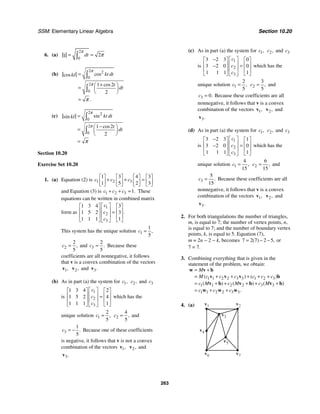
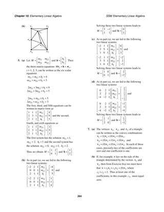
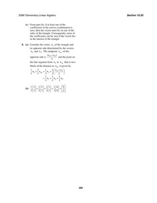
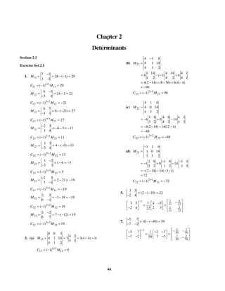
![SSM: Elementary Linear Algebra Section 2.1
45
9.
2
2
3 5
3 2 5 3
3 2
5 6 15
5 21
( )( ) ( )( )
a
a a
a
a a
a a
−
= − − − −
− −
= − + +
= − +
11.
2 1 4 2 1 4 2 1
3 5 7 3 5 7 3 5
1 6 2 1 6 2 1 6
2 5 2 1 7 1 4 3 6 4 5 1 2 7 6 1 3 2
20 7 72 20 84 6
65
[( )( )( ) ( )( )( ) ( )( )( )] [( )( )( ) ( )( )( ) ( )( )( )]
[ ] [ ]
− − −
− = −
= − + − + − + − − +
= − − + − + +
= −
13.
3 0 0 3 0 0 3 0
2 1 5 2 1 5 2 1
1 9 4 1 9 4 1 9
3 1 4 0 5 1 0 2 9 0 1 1 3 5 9 0 2 4
12 135
123
[( )( )( ) ( )( )( ) ( )( )( )] [ ( )( ) ( )( )( ) ( )( )( )]
− = − −
− −
= − − + + − − + + −
= −
= −
15.
2
2
2 4 5
2 8 5
2 3
1 3
det( ) ( )( ) ( )
( )( )
A = λ − λ + − −
= λ + λ − +
= λ + λ −
= λ − λ +
det(A) = 0 for λ = 1 or −3.
17. det(A) = (λ − 1)(λ + 1) − 0 = (λ − 1)(λ + 1)
det(A) = 0 for λ = 1 or −1.
19. (a)
3 0 0
1 5 2 5 2 1
2 1 5 3 0 0
9 4 1 4 1 9
1 9 4
3 4 45
123
( )
− −
− = − +
− −
−
= −
= −
(b)
3 0 0
1 5 0 0 0 0
2 1 5 3 2 1
9 4 9 4 1 5
1 9 4
3 4 45 2 0 0 0 0
123
( ) ( ) ( )
−
− = − +
− − −
−
= − − − + −
= −
(c)
3 0 0
0 0 3 0 3 0
2 1 5 2 1 5
9 4 1 4 1 9
1 9 4
2 0 0 12 0 5 27 0
12 135
123
( )
( ) ( ) ( )
− = − + − −
− −
−
= − − − − − − −
= −
= −](https://image.slidesharecdn.com/elementary-linear-algebra-chapter1-220420115526/85/Elementary-linear-algebra-chapter-1-pdf-100-320.jpg)
![Chapter 2: Determinants SSM: Elementary Linear Algebra
46
(d)
3 0 0
2 5 3 0 3 0
2 1 5 0 1 9
1 4 1 4 2 5
1 9 4
12 0 9 15 0
12 135
123
( )
( ) ( )
− = − + − −
− −
−
= − − − − −
= −
= −
(e)
3 0 0
0 0 3 0 3 0
2 1 5 1 9 4
1 5 2 5 2 1
1 9 4
0 0 9 15 0 4 3 0
135 12
123
( )
( ) ( ) ( )
− = − + −
− −
−
= − − − − − −
= − +
= −
(f)
3 0 0
2 1 3 0 3 0
2 1 5 0 5 4
1 9 1 9 2 1
1 9 4
5 27 0 4 3 0
135 12
123
( )
( ) ( )
−
− = − + −
−
−
= − − − − −
= − +
= −
21. Expand along the second column.
3 7
5 5 15 7 40
1 5
det( ) [ ( )]
A
−
= = − − − = −
−
23. Expand along the first column.
2 2 2
2 2 2
3 3 3 3 3 3
1 1 1
0
det( )
( ) ( ) ( )
k k k k k k
A
k k k k k k
k k k k k k
= − +
= − − − + −
=
25. Expand along the third column, then along the first rows of the 3 × 3 matrices.
3 3 5 3 3 5
3 2 2 2 3 2 2 2
2 10 2 4 1 0
2 2 2 2 2 2 2 2 2 2 2 2
3 3 3 5 3 3 3 5
10 2 2 2 2 10 1 0 4 0 4 1
3 3 24 3 8 5 16 3 3 2 3 8 5 6
3 128 3 48
240
det( )
[ ( ) ( ) ( )] [ ( ) ( ) ( )]
( ) ( )
A = − − − −
⎛ ⎞ ⎛ ⎞
− − − −
= − + − − +
⎜ ⎟ ⎜ ⎟
⎝ ⎠ ⎝ ⎠
= − − + − − + −
= − − −
= −
27.
1 0 0
0 1 0 1 1 1 1
0 0 1
( )( )( )
− = − = −](https://image.slidesharecdn.com/elementary-linear-algebra-chapter1-220420115526/85/Elementary-linear-algebra-chapter-1-pdf-101-320.jpg)
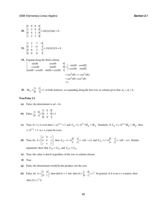
![Chapter 2: Determinants SSM: Elementary Linear Algebra
48
(i) False; let
1 0
0 1
A
⎡ ⎤
= ⎢ ⎥
⎣ ⎦
and
1 0
0 1
,
B
−
⎡ ⎤
= ⎢ ⎥
−
⎣ ⎦
then
det(A) = det(B) = 1, but det(A + B) = 0.
(j) True; let
a b
A
c d
⎡ ⎤
= ⎢ ⎥
⎣ ⎦
so that
2
2
2
a bc ab bd
A
ac cd bc d
⎡ ⎤
+ +
= ⎢ ⎥
+ +
⎢ ⎥
⎣ ⎦
and
2 2 2
2 2 2 2 2 2 2 2
2 2 2 2
2
2
2
2
det( ) ( )( ) ( )( )
( )
( )
(det( ))
A a bc bc d ab bd ac cd
a bc a d bcd b c a bc abcd bcd
a d abcd b c
ad bc
A
= + + − + +
= + + + − + +
= − +
= −
=
Section 2.2
Exercise Set 2.2
1. det(A) = (−2)(4) − (3)(1) = −8 − 3 = −11
2 1
3 4
T
A
−
⎡ ⎤
= ⎢ ⎥
⎣ ⎦
2 4 1 3 8 3 11
det( ) ( )( ) ( )( )
T
A = − − = − − = −
3. 2 2 6 1 4 5 3 1 3 3 2 5 2 4 3 1 1 6
24 20 9 30 24 6
5
det( ) [( )( )( ) ( )( )( ) ( )( )( )] [( )( )( ) ( )( )( ) ( )( )( )]
[ ] [ ]
A = + − + − − + − + −
= − − − − −
= −
2 2 6 1 3 3 5 1 4 5 2 3 2 3 4 1 1 6
24 9 20 30 24 6
5
det( ) [( )( )( ) ( )( )( ) ( )( )( )] [( )( )( ) ( )( )( ) ( )( )( )]
[ ] [ ]
T
A = + − + − − + − + −
= − − − − −
= −
5. The matrix is 4
I with the third row multiplied by −5.
1 0 0 0
0 1 0 0
5
0 0 5 0
0 0 0 1
= −
−
7. The matrix is 4
I with the second and third rows interchanged.
1 0 0 0
0 0 1 0
1
0 1 0 0
0 0 0 1
= −
9. The matrix is 4
I with −9 times the fourth row added to the second row.
1 0 0 0
0 1 0 9
1
0 0 1 0
0 0 0 1
−
=](https://image.slidesharecdn.com/elementary-linear-algebra-chapter1-220420115526/85/Elementary-linear-algebra-chapter-1-pdf-103-320.jpg)
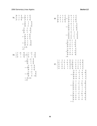
![Chapter 2: Determinants SSM: Elementary Linear Algebra
50
19. Exercise 14: First add multiples of the first row
to the remaining rows, then expand by cofactors
along the first column. Repeat these steps with
the 3 × 3 determinant, then evaluate the 2 × 2
determinant.
1 2 3 1 1 2 3 1
5 9 6 3 0 1 9 2
1 2 6 2 0 0 3 1
2 8 6 1 0 12 0 1
1 9 2
0 3 1
12 0 1
1 9 2
0 3 1
0 108 23
3 1
108 23
3 23 1 108
39
( )( ) ( )( )
− −
− − −
=
− − − − −
−
− −
= − −
−
− −
= − −
− −
=
= − − −
=
Exercise 15: Add −2 times the second row to the
first row, then expand by cofactors along the
first column. For the 3 × 3 determinant, add
multiples of the first row to the remaining row,
then expand by cofactors of the first column.
Finally, evaluate the 2 × 2 determinant.
2 1 3 1 0 1 1 1
1 0 1 1 1 0 1 1
0 2 1 0 0 2 1 0
0 1 2 2 0 1 2 3
1 1 1
1 2 1 0
1 2 3
1 1 1
0 1 2
0 1 4
1 2
1 4
4 2
6
( )
( )
−
=
−
= −
−
= − −
−
= −
= − − −
=
Exercise 16: Add
1
2
− times the first row to the
second row, then expand by cofactors along the
fourth column. For the 3 × 3 determinant, add −2
times the second row to the third row, then
expand by cofactors along the second column.
Finally, evaluate the 2 × 2 determinant.
1 1 1 1 1
2 2 2 2 2
2 1 1 2 1 1
3 3 3 3 3 3
1 2 1 2
3 3 3 3
1 1
2 2
2 1 1
3 3 3
1 2
3 3
1 1
2 2
2 1 1
3 3 3
5 2
3 3
1 1
2 2
5 2
3 3
0 1 1 1 0 1 1 1
1 0 0
0 0
0 0 0 0
0
1
0
0
0
1
3
1 1 5
3 3 6
1
6
( )
=
− −
= −
−
= −
− −
⎛ ⎞
= −⎜ ⎟
− −
⎝ ⎠
⎡ ⎤
⎛ ⎞
= − − − −
⎜ ⎟
⎢ ⎥
⎝ ⎠
⎣ ⎦
= −
Exercise 17: Add 2 times the first row to the
second row, then expand by cofactors along the
first column two times. For the 3 × 3
determinant, add −2 times the first row to the
second row, then expand by cofactors along the
first column. Finally, evaluate the 2 × 2
determinant.
1 3 1 5 3 1 3 1 5 3
2 7 0 4 2 0 1 2 6 8
0 0 1 0 1 0 0 1 0 1
0 0 2 1 1 0 0 2 1 1
0 0 0 1 1 0 0 0 1 1
1 2 6 8
0 1 0 1
0 2 1 1
0 0 1 1
1 0 1
1 2 1 1
0 1 1
1 0 1
0 1 1
0 1 1
1 1
1 1
1 1
2
( )
[ ( )]
− − − −
=
−
=
= −
= − −
−
= −
= − − −
= −](https://image.slidesharecdn.com/elementary-linear-algebra-chapter1-220420115526/85/Elementary-linear-algebra-chapter-1-pdf-105-320.jpg)
![SSM: Elementary Linear Algebra Section 2.3
51
21. Interchange the second and third rows, then the
first and second rows to arrive at the determinant
whose value is given.
6
d e f d e f a b c
g h i a b c d e f
a b c g h i g h i
= − = = −
23. Remove the common factors of 3 from the first
row, −1 from the second row, and 4 from the
third row to arrive at the determinant whose
value is given.
3 3 3
3
4 4 4 4 4 4
3
4 4 4
12
12 6
72
( )
a b c a b c
d e f d e f
g h i g h i
a b c
d e f
g h i
a b c
d e f
g h i
− − − = − − −
= −
= −
= − −
=
25. Add −1 times the third row to the first row to
arrive at the matrix whose value is given.
6
a g b h c i a b c
d e f d e f
g h i g h i
+ + +
= = −
27. Remove the common factor of −3 from the first
row, then add 4 times the second row to the third
to arrive at the matrix whose value is given.
3 3 3
4 4 4
3
4 4 4
3
3 6
18
( )
a b c
d e f
g d h e i f
a b c
d e f
g d h e i f
a b c
d e f
g h i
− − −
− − −
= −
− − −
= −
= − −
=
29.
2 2 2
2 2 2 2
2 2 2 2
2 2 2 2
1 1 1
1 1 1
0
0
( )( ) ( )( )
( )( )( ) ( )( )( )
( )( )[ ( )]
( )( )( )
a b c
a b c
b a c a
b a c a
b a c a
b a c a
b a c a c a b a
b a c a c a c a b a b a
b a c a c a b a
b a c a c b
= − −
− −
− −
=
− −
= − − − − −
= − + − − − + −
= − − + − +
= − − −
True/False 2.2
(a) True; interchanging two rows of a matrix causes
the determinant to be multiplied by −1, so two
such interchanges result in a multiplication by
(−1)(−1) = 1.
(b) True; consider the transposes of the matrices so
that the column operations performed on A to get
B are row operations on .
T
A
(c) False; adding a multiple of one row to another
does not change the determinant. In this case,
det(B) = det(A).
(d) False; multiplying each row by its row number
causes the determinant to be multiplied by the
row number, so det(B) = n! det(A).
(e) True; since the columns are identical, they are
proportional, so det(A) = 0 by Theorem 2.2.5.
(f) True; −1 times the second and fourth rows can
be added to the sixth row without changing
det(A). Since this introduces a row of zeros,
det(A) = 0.
Section 2.3
Exercise Set 2.3
1. det(A) = −4 − 6 = −10
2
2 4
2 16 24 40 2 10
6 8
det( ) ( )
A
−
= = − − = − = −](https://image.slidesharecdn.com/elementary-linear-algebra-chapter1-220420115526/85/Elementary-linear-algebra-chapter-1-pdf-106-320.jpg)
![Chapter 2: Determinants SSM: Elementary Linear Algebra
52
3. det(A) = [20 − 1 + 36] − [6 + 8 − 15] = 56
3
4 2 6
2 6 4 2
2 8 10
160 8 288 48 64 120
448
2 56
det( )
[ ] [ ]
( ) ( )
A
− −
− = − − −
− − −
= − + − − − − +
= −
= −
5.
9 1 8
31 1 17
10 0 2
18 170 0 80 0 62
170
det( )
[ ] [ ]
AB
−
=
= − − − + −
= −
1 3 6
17 11 4
10 5 2
22 120 510 660 20 102
170
det( )
[ ] [ ]
BA
− −
=
= − − + − − −
= −
2 1
2 2 8 3 10
3 4
det( ) ( )
A = = − =
1 10 0 15 0 7 17
det( ) [ ] [ ]
B = − + − + − = −
3 0 3
10 5 2
5 0 3
3 3
5
5 3
5 9 15
30
det( )
( )
det( ) det( )
A B
A B
+ =
=
= −
= −
≠ +
7. Add multiples of the second row to the first and
third row to simplify evaluating the determinant.
0 3 5
3 5
1 1 0 1 9 10 1
2 3
0 2 3
det( ) ( )
A = − − = − − = − = −
Since det(A) ≠ 0, A is invertible.
9. Expand by cofactors of the first column.
1 3
2 2 2 4
0 2
det( ) ( )
A
−
= = =
Since det(A) ≠ 0, A is invertible.
11. The third column of A is twice the first column,
so det(A) = 0 and A is not invertible.
13. Expand by cofactors of the first row.
1 0
2 2 6 12
3 6
det( ) ( )
A = = =
Since det(A) ≠ 0, A is invertible.
15.
2
2
3 2 4
5 6 4
5 2
det( ) ( )( )
A k k
k k
k k
= − − −
= − + −
= − +
Use the quadratic formula to solve
2
5 2 0.
k k
− + =
2
5 5 4 1 2 5 17
2 1 2
( ) ( ) ( )( )
( )
k
− − ± − − ±
= =
A is invertible for
5 17
2
.
k
±
≠
17. 2 12 36 4 18 12
8 8
det( ) [ ] [ ]
A k k
k
= + + − + +
= +
A is invertible for k ≠ −1.
19. A is the same matrix as in Exercise 7, which was
shown to be invertible (det(A) = −1). The
cofactors of A are 11 3,
C = − 12 3 3
( ) ,
C = − − =
13 4 2 2,
C = − + = − 21 15 20 5
( ) ,
C = − − =
22 6 10 4,
C = − = − 23 8 10 2
( ) ,
C = − − =
31 0 5 5,
C = + = 32 0 5 5
( ) ,
C = − + = − and
33 2 5 3.
C = − + =
The matrix of cofactors is
3 3 2
5 4 2
5 5 3
.
− −
⎡ ⎤
⎢ ⎥
−
⎢ ⎥
−
⎣ ⎦
1
3 5 5
1 1
adj 3 4 5
1 2 2 3
3 5 5
3 4 5
2 2 3
( )
det( )
A A
A
−
−
⎡ ⎤
⎢ ⎥
= = − −
⎢ ⎥
− −
⎣ ⎦
− −
⎡ ⎤
⎢ ⎥
= −
⎢ ⎥
− −
⎣ ⎦
21. A is the same matrix as in Exercise 9, which was
shown to be invertible (det(A) = 4). The
cofactors of A are 11 2,
C = 12 0,
C = 13 0,
C =
21 6 6
( ) ,
C = − − = 22 4,
C = 23 0,
C =
31 9 5 4,
C = − = 32 6 6
( ) ,
C = − − = and 33 2.
C =](https://image.slidesharecdn.com/elementary-linear-algebra-chapter1-220420115526/85/Elementary-linear-algebra-chapter-1-pdf-107-320.jpg)
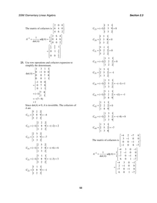
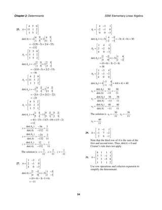
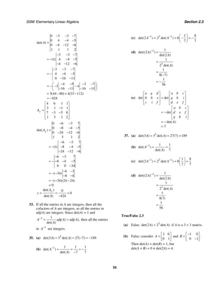
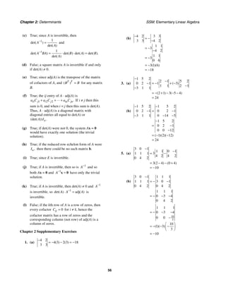
![SSM: Elementary Linear Algebra Chapter 2 Supplementary Exercises
57
7. (a)
3 6 0 1
3 1 4 2 1 4 2 3 1
2 3 1 4
3 0 1 1 6 1 1 1 1 1 0 1
1 0 1 1
2 2 2 9 2 2 9 2 2
9 2 2 2
1 1 1 4 1 1 1 1 1 1 3 1 2 3
3 3 2 6 2 1 4 1 1
2 2 1 1 2 2 9 2 9 2 2 2 9 2
3 3 2 2 2 1 4 6 2 2 2 2 9 4 2 9 6 2 4
( )
[ ( ) ( )] [ ( ) ( ) ( )] [ ( ) (
− −
−
= − − − − −
−
− − − − −
− −
⎛ ⎞ ⎛ ⎞ ⎛ ⎞
− − − −
= + − − − + − − − −
⎜ ⎟ ⎜ ⎟ ⎜ ⎟
− − − − − − − −
⎝ ⎠ ⎝ ⎠ ⎝ ⎠
= − + + + − − − + − + + − − − − − − + − + 27
30 330 31
329
)]
= + −
=
(b)
31
3
329
15
3 6 0 1 1 0 1 1
2 3 1 4 2 3 1 4
1 0 1 1 3 6 0 1
9 2 2 2 9 2 2 2
1 0 1 1
0 3 1 6
0 6 3 2
0 2 11 11
1 0 1 1
0 3 1 6
0 0 5 14
0 0 7
1 0 1 1
0 3 1 6
0 0 5 14
0 0 0
329
1 3 5
15
329
( )( )( )
−
− −
= −
−
− − − −
−
−
= −
−
−
−
−
= − −
−
−
−
= − −
−
⎛ ⎞
= − −
⎜ ⎟
⎝ ⎠
=
9. Exercise 3:
1 5 2 1 5 2 1 5
0 2 1 0 2 1 0 2
3 1 1 3 1 1 3 1
1 2 1 5 1 3 2 0 1 2 2 3 1 1 1 5 0 1
13 11
24
[( )( )( ) ( )( )( ) ( )( )( )] [( )( )( ) ( )( )( ) ( )( )( )]
( )
− − −
− = −
− − −
= − + − − + − − + − − +
= − −
=
Exercise 4:
1 2 3 1 2 3 1 2
4 5 6 4 5 6 4 5
7 8 9 7 8 9 7 8
1 5 9 2 6 7 3 4 8 3 5 7 1 6 8 2 4 9
225 225
0
[( )( )( ) ( )( )( ) ( )( )( )] [( )( )( ) ( )( )( ) ( )( )( )]
( )
− − − − − − − −
− − − = − − − − −
− − − − − − − −
= − − − + − − − + − − − − − − − + − − − + − − −
= − − −
=](https://image.slidesharecdn.com/elementary-linear-algebra-chapter1-220420115526/85/Elementary-linear-algebra-chapter-1-pdf-112-320.jpg)
![Chapter 2: Determinants SSM: Elementary Linear Algebra
58
Exercise 5:
3 0 1 3 0 1 3 0
1 1 1 1 1 1 1 1
0 4 2 0 4 2 0 4
3 1 2 0 1 0 1 1 4 1 1 0 3 1 4 0 1 2
2 12
10
[( )( )( ) ( )( )( ) ( )( )( )] [( )( )( ) ( )( )( ) ( )( )( )]
− −
=
= + + − − − + +
= −
= −
Exercise 6:
5 1 4 5 1 4 5 1
3 0 2 3 0 2 3 0
1 2 2 1 2 2 1 2
5 0 2 1 2 1 4 3 2 4 0 1 5 2 2 1 3 2
22 26
48
[( )( )( ) ( )( )( ) ( )( )( )] [( )( )( ) ( )( )( ) ( )( )( )]
− − −
=
− − −
= − + + − − + − − +
= − −
= −
11. The determinants for Exercises 1, 3, and 4 were evaluated in Exercises 1, 3, and 9.
Exercise 2:
7 1
7 6 1 2 44
2 6
( ) ( )( )
−
= − − − − = −
− −
The determinants of the matrices in Exercises 1−3 are nonzero, so those matrices are invertible. The matrix in
Exercise 4 is not invertible, since its determinant is zero.
13.
2
2
5 3
5 3 3 2
2 3
15 5 6
5 21
( ) ( )( )
b
b b
b
b b
b b
−
= − − − −
− −
= − − + −
= − + −
15.
0 0 0 0 3
0 0 0 4 0
5 2 1 4 3
0 0 1 0 0
0 2 0 0 0
5 0 0 0 0
120
( )( )( )( )( )
−
−
= − − −
−
= −
17. Let
4 2
3 3
.
A
−
⎡ ⎤
= ⎢ ⎥
⎣ ⎦
Then det(A) = −18. The cofactors of A are 11 3,
C = 12 3,
C = − 21 2,
C = − and 22 4.
C = − The
matrix of cofactors is
3 3
2 4
.
−
⎡ ⎤
⎢ ⎥
− −
⎣ ⎦
1 1
1 6 9
1 2
6 9
1 1 3 2
adj
3 4
18
( )
det( )
A A
A
−
⎡ ⎤
−
−
⎡ ⎤ ⎢ ⎥
= = =
⎢ ⎥
− −
− ⎣ ⎦ ⎢ ⎥
⎣ ⎦
19. Let
1 5 2
0 2 1
3 1 1
.
A
−
⎡ ⎤
⎢ ⎥
= −
⎢ ⎥
−
⎣ ⎦
Then det(A) = 24.
The cofactors of A are 11 2 1 3,
C = + = 12 0 3 3
( ) ,
C = − − = 13 0 6 6,
C = + = 21 5 2 3
( ) ,
C = − − = − 22 1 6 5,
C = − + =
23 1 15 14
( ) ,
C = − − + = − 31 5 4 9,
C = − − = − 32 1 0 1
( ) ,
C = − − = − and 33 2 0 2.
C = − − = −](https://image.slidesharecdn.com/elementary-linear-algebra-chapter1-220420115526/85/Elementary-linear-algebra-chapter-1-pdf-113-320.jpg)
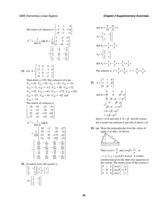
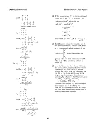
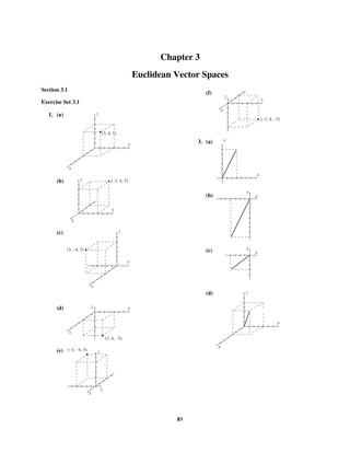
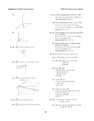
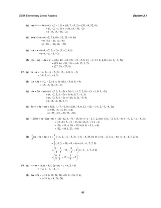
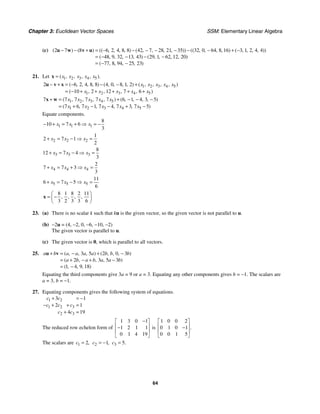
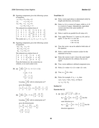
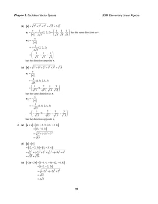
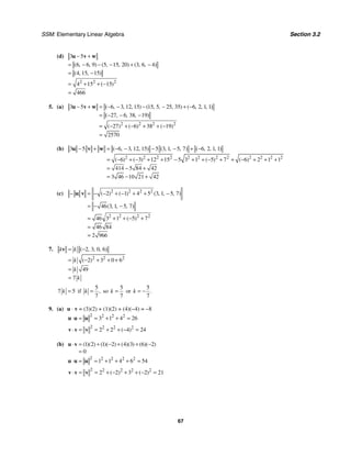
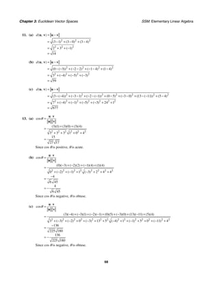
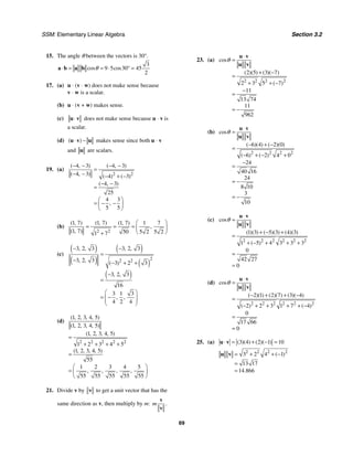
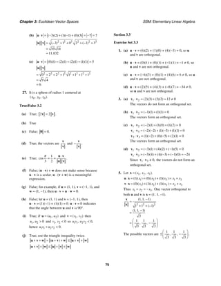
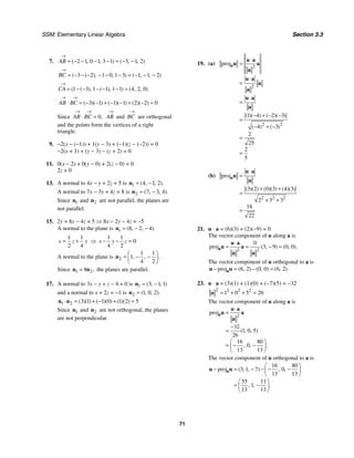
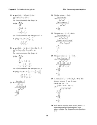
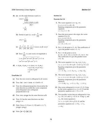
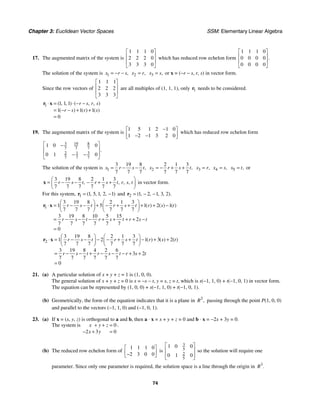
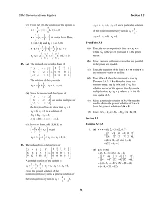
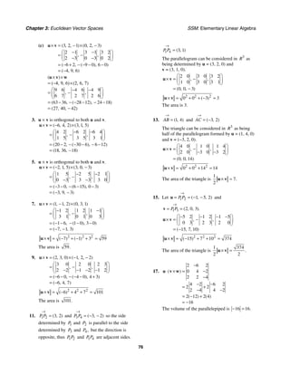
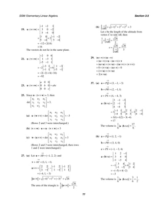
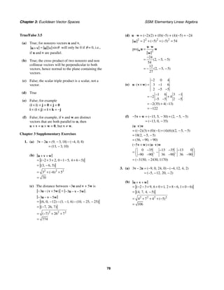
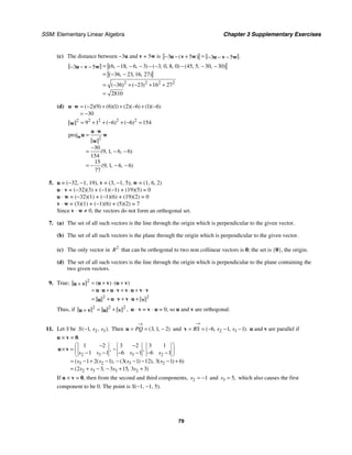
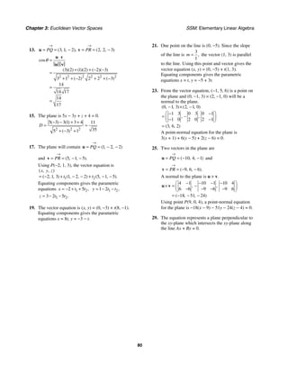
![81
Chapter 4
General Vector Spaces
Section 4.1
Exercise Set 4.1
1. (a) 1 2 3 4
1 3 2 4
2 6
( , ) ( , )
( , )
( , )
+ = − +
= − + +
=
u v
3u = 3(−1, 2) = (0, 6)
(b) The sum of any two real numbers is a real number. The product of two real numbers is a real number and 0 is
a real number.
(c) Axioms 1−5 hold in V because they also hold in 2
.
R
(e) Let 1 2
( , )
u u
=
u with 1 0.
u ≠ Then 1 2 2
1 1 0
( , ) ( , ) .
u u u
= = ≠
u u
3. The set is a vector space with the given operations.
5. The set is not a vector space. Axiom 5 fails to hold because of the restriction that x ≥ 0. Axiom 6 fails to hold for
k 0.
7. The set is not a vector space. Axiom 8 fails to hold because 2 2 2
( ) .
k m k m
+ ≠ +
9. The set is a vector space with the given operations.
11. The set is a vector space with the given operations.
23. Hypothesis
Add to both sides.
Axiom 3
Axiom 5
Axiom 4
( ) ( ) ( ) ( )
[ ( )] [ ( )]
+ = +
+ + − = + + − −
+ + − = + + −
+ = +
=
u w v w
u w w v w w w
u w w v w w
u 0 v 0
u v
25. (1) Axiom 7
(2) Axiom 4
(3) Axiom 5
(4) Axiom 1
(5) Axiom 3
(6) Axiom 5
(7) Axiom 4
True/False 4.1
(a) False; vectors are not restricted to being directed line segments.
(b) False; vectors are not restricted to being n-tuples of real numbers.
(c) True](https://image.slidesharecdn.com/elementary-linear-algebra-chapter1-220420115526/85/Elementary-linear-algebra-chapter-1-pdf-136-320.jpg)
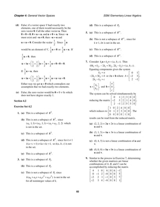
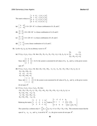
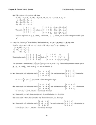
![SSM: Elementary Linear Algebra Section 4.3
85
(f) Since det(A) = 0, reduce the matrix
1 3 1 0
2 6 2 0
3 9 3 0
.
−
⎡ ⎤
⎢ ⎥
−
⎢ ⎥
−
⎣ ⎦
The matrix reduces to
1 3 1 0
0 0 0 0
0 0 0 0
.
−
⎡ ⎤
⎢ ⎥
⎢ ⎥
⎣ ⎦
The solution set
is x − 3y + z = 0, which is a plane through the origin.
17. Let f = f(x) and g = g(x) be elements of the set. Then
0
( ( ) ( ))
( ) ( )
b
a
b b
a a
f x g x dx
f x dx g x dx
+ = +
= +
=
∫
∫ ∫
f g
and f + g is in the set. Let k be any scalar. Then 0 0
( ) ( )
b b
a a
k kf x dx k f x dx k
= = = ⋅ =
∫ ∫
f so kf is in the set. Thus
the set is a subspace of C[a, b].
True/False 4.2
(a) True; this is part of the definition of a subspace.
(b) True; since a vector space is a subset of itself.
(c) False; for instance, the set W in Example 4 contains the origin (zero vector), but is not a subspace of 2
.
R
(d) False; 2
R is not a subset of 3
.
R
(e) False; if b ≠ 0, i.e., the system is not homogeneous, then the solution set does not contain the zero vector.
(f) True; this is by the definition of the span of a set of vectors.
(g) True; by Theorem 4.2.2.
(h) False; consider the subspaces { }
1 ( , )
W x y y x
= = and { }
2 ( , )
W x y y x
= = − in 2
.
R 1 1 1
( , )
=
v is in 1
W and
2 1 1
( , )
= −
v is in 2,
W but 1 2 2 0
( , )
+ =
v v is not in { }
1 2 ( , ) .
W W x y y x
∪ = = ±
(i) False; let 1 1 0
( , ),
=
v 2 0 1
( , ),
=
v 1 1 0
( , ),
= −
u and 2 0 1
( , ).
= −
u Then 1 2
{ , }
v v and 1 2
{ , }
u u both span 2
R but
1 2 1 2
{ , } { , }.
≠
u u v v
(j) True; the sum of two upper triangular matrices is upper triangular and the scalar multiple of an upper triangular
matrix is upper triangular.
(k) False; the span of x − 1, 2
1
( ) ,
x − and 3
1
( )
x − will only contain polynomials for which p(1) = 0, i.e., not all of 3.
P
Section 4.3
Exercise Set 4.3
1. (a) 2 1
5 ,
= −
u u i.e., 2
u is a scalar multiple of 1.
u
(b) Since there are 3 vectors and 3 2, the set is linearly dependent by Theorem 4.3.3.
(c) 2 1
2 ,
=
p p i.e., 2
p is a scalar multiple of 1.
p](https://image.slidesharecdn.com/elementary-linear-algebra-chapter1-220420115526/85/Elementary-linear-algebra-chapter-1-pdf-140-320.jpg)
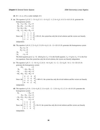
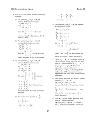

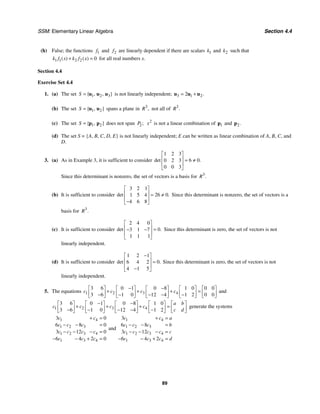
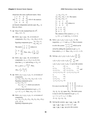
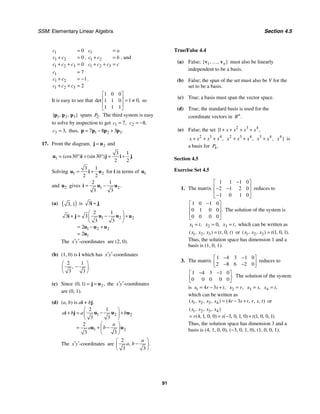
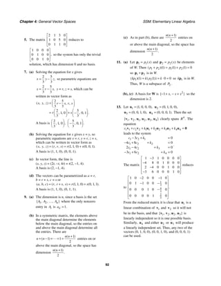
![SSM: Elementary Linear Algebra Section 4.6
93
15. Let 3 ( , , ).
a b c
=
v The equation
1 1 2 2 3 3
c c c
+ + =
v v v 0 leads to the system
1 3
1 2 3
1 2 3
0
2 5 0
3 3 0
c ac
c c bc
c c cc
+ =
− + + =
− + =
.
The matrix
1 0 0
2 5 0
3 3 0
a
b
c
⎡ ⎤
⎢ ⎥
−
⎢ ⎥
−
⎣ ⎦
reduces to
2 1
5 5
9 3
5 5
1 0 0
0 1 0
0 0 0
a
a b
a b c
⎡ ⎤
⎢ ⎥
+
⎢ ⎥
⎢ ⎥
− + +
⎣ ⎦
and the
homogeneous system has only the trivial
solution if
9 3
0
5 5
.
a b c
− + + ≠ Thus, adding any
vector 3 ( , , )
a b c
=
v with 9a − 3b − 5c ≠ 0 will
create a basis for 3
.
R
True/False 4.5
(a) True; by definition.
(b) True; any basis of 17
R will contain 17 linearly
independent vectors.
(c) False; to span 17
,
R at least 17 vectors are
required.
(d) True; since the dimension for 5
R is 5, then
linear independence is sufficient for 5 vectors to
be a basis.
(e) True; since the dimension of 5
R is 5, then
spanning is sufficient for 5 vectors to be a basis.
(f) True; if the set contains n vectors, it is a basis,
while if it contains more than n vectors, it can be
reduced to a basis.
(g) True; if the set contains n vectors, it is a basis,
while if it contains fewer than n vectors, it can be
enlarged to a basis.
(h) True; the set
1 0 1 0 0 1 0 1
0 1 0 1 1 0 1 0
, , ,
⎧ ⎫
⎡ ⎤ ⎡ ⎤ ⎡ ⎤ ⎡ ⎤
⎨ ⎬
⎢ ⎥ ⎢ ⎥ ⎢ ⎥ ⎢ ⎥
− −
⎣ ⎦ ⎣ ⎦ ⎣ ⎦ ⎣ ⎦
⎩ ⎭
form a
basis for 22.
M
(i) True; the set of n × n matrices has dimension
2
,
n while the set
2
2
{ , , , , }
n
I A A A
… contains
2
1
n + matrices.
(j) False; since 2
P has dimension three, then by
Theorem 4.5.6(c), the only three-dimensional
subspace of 2
P is 2
P itself.
Section 4.6
Exercise Set 4.6
1. (a) Since 1 2
{ , }
u u is the standard basis B for
2
,
R
3
7
[ ] .
s
⎡ ⎤
= ⎢ ⎥
−
⎣ ⎦
w
(b)
2 3 1 0
4 8 0 1
⎡ ⎤
⎢ ⎥
−
⎣ ⎦
reduces to
3
2
7 28
1 1
7 14
1 0
0 1
.
⎡ ⎤
−
⎢ ⎥
⎢ ⎥
⎣ ⎦
Thus
3
2
7 28
1 1
7 14
B S
P →
⎡ ⎤
−
⎢ ⎥
=
⎢ ⎥
⎣ ⎦
and
3 5
2
7 28 28
1 1 3
7 14 14
1
1
[ ] [ ] .
S B S B
P →
⎡ ⎤ ⎡ ⎤
− ⎡ ⎤
⎢ ⎥ ⎢ ⎥
= = =
⎢ ⎥
⎢ ⎥ ⎣ ⎦ ⎢ ⎥
⎣ ⎦ ⎣ ⎦
w w
(c)
1 0 1 0
1 2 0 1
⎡ ⎤
⎢ ⎥
⎣ ⎦
reduces to 1 1
2 2
1 0 1 0
0 1
.
⎡ ⎤
⎢ ⎥
−
⎣ ⎦
Thus 1 1
2 2
1 0
B S
P →
⎡ ⎤
= ⎢ ⎥
−
⎣ ⎦
and
1 1
2 2
1 1
2 2
1 0
[ ] [ ]
.
S B S B
P
a
b
a
a b
→
=
⎡ ⎤ ⎡ ⎤
= ⎢ ⎥ ⎢ ⎥
− ⎣ ⎦
⎣ ⎦
⎡ ⎤
= ⎢ ⎥
− +
⎣ ⎦
w w
3. (a) Since S is the standard basis B for 2,
P
4 3 1
( ) ( , , )
S = −
p or
4
3
1
[ ] .
S
⎡ ⎤
⎢ ⎥
= −
⎢ ⎥
⎣ ⎦
p](https://image.slidesharecdn.com/elementary-linear-algebra-chapter1-220420115526/85/Elementary-linear-algebra-chapter-1-pdf-148-320.jpg)
![Chapter 4: General Vector Spaces SSM: Elementary Linear Algebra
94
(b)
1 1 0 1 0 0
1 0 1 0 1 0
0 1 1 0 0 1
⎡ ⎤
⎢ ⎥
⎢ ⎥
⎣ ⎦
reduces to
1 1 1
2 2 2
1 1 1
2 2 2
1 1 1
2 2 2
1 0 0
0 1 0
0 0 1
.
⎡ ⎤
−
⎢ ⎥
−
⎢ ⎥
⎢ ⎥
−
⎢ ⎥
⎣ ⎦
Thus,
1 1 1
2 2 2
1 1 1
2 2 2
1 1 1
2 2 2
B S
P →
⎡ ⎤
−
⎢ ⎥
= −
⎢ ⎥
⎢ ⎥
−
⎢ ⎥
⎣ ⎦
and
1 1 1
2 2 2
1 1 1
2 2 2
1 1 1
2 2 2
2
1
1
0
2
1
[ ] [ ]
S B S B
P →
=
⎡ ⎤
−
⎡ ⎤
⎢ ⎥
⎢ ⎥
= −
⎢ ⎥ −
⎢ ⎥
⎢ ⎥
⎣ ⎦
−
⎢ ⎥
⎣ ⎦
⎡ ⎤
⎢ ⎥
=
⎢ ⎥
−
⎣ ⎦
p p
or 0 2 1
( ) ( , , ).
S = −
p
5. (a) From Theorem 4.6.2,
1 2 3
0 2 3
0 0 3
S B
P →
⎡ ⎤
⎢ ⎥
=
⎢ ⎥
⎣ ⎦
where B is the standard basis for 3
.
R Thus,
1 2 3 6 16
0 2 3 1 10
0 0 3 4 12
[ ] [ ]
B S B S
P →
⎡ ⎤ ⎡ ⎤ ⎡ ⎤
⎢ ⎥ ⎢ ⎥ ⎢ ⎥
= = =
−
⎢ ⎥ ⎢ ⎥ ⎢ ⎥
⎣ ⎦ ⎣ ⎦ ⎣ ⎦
w w
and w = (16, 10, 12).
(b) The basis in Exercise 3(a) is the standard
basis B for 2,
P so
3
0
4
[ ] [ ]
B S
⎡ ⎤
⎢ ⎥
= =
⎢ ⎥
⎣ ⎦
q q and
2
3 4 .
x
= +
q
(c) From Theorem 4.6.2,
1 1 0 0
1 1 0 0
0 0 1 0
0 0 0 1
S E
P →
−
⎡ ⎤
⎢ ⎥
= ⎢ ⎥
⎢ ⎥
⎢ ⎥
⎣ ⎦
where E is the
standard basis for 22.
M
Thus,
1 1 0 0 8
1 1 0 0 7
0 0 1 0 6
0 0 0 1 3
15
1
6
3
[ ] [ ]
E S E S
B P B
→
− −
⎡ ⎤ ⎡ ⎤
⎢ ⎥ ⎢ ⎥
= = ⎢ ⎥ ⎢ ⎥
⎢ ⎥ ⎢ ⎥
⎢ ⎥ ⎢ ⎥
⎣ ⎦ ⎣ ⎦
⎡ ⎤
⎢ ⎥
−
= ⎢ ⎥
⎢ ⎥
⎢ ⎥
⎣ ⎦
and
15 1
6 3
.
B
−
⎡ ⎤
= ⎢ ⎥
⎣ ⎦
7. (a)
2 4 1 1
2 1 3 1
−
⎡ ⎤
⎢ ⎥
− −
⎣ ⎦
reduces to
13 1
10 2
2
5
1 0
0 1 0
⎡ ⎤
−
⎢ ⎥
−
⎢ ⎥
⎣ ⎦
so
13 1
10 2
2
5
0
.
B B
P ′→
⎡ ⎤
−
⎢ ⎥
=
−
⎢ ⎥
⎣ ⎦
(b)
1 1 2 4
3 1 2 1
−
⎡ ⎤
⎢ ⎥
− −
⎣ ⎦
reduces to
5
2
13
2
1 0 0
0 1 2
⎡ ⎤
−
⎢ ⎥
− −
⎢ ⎥
⎣ ⎦
so
5
2
13
2
0
2
.
B B
P ′
→
⎡ ⎤
−
⎢ ⎥
=
− −
⎢ ⎥
⎣ ⎦
(c)
2 4 1 0
2 1 0 1
⎡ ⎤
⎢ ⎥
−
⎣ ⎦
reduces to
1 2
10 5
1 1
5 5
1 0
0 1
⎡ ⎤
⎢ ⎥
−
⎢ ⎥
⎣ ⎦
so
1 2
10 5
1 1
5 5
E B
P →
⎡ ⎤
⎢ ⎥
=
−
⎢ ⎥
⎣ ⎦
where E is the standard basis for 2
.
R
1 2
10 5
1 1
5 5
17
10
8
5
3
5
[ ] [ ]
B E B E
P →
=
⎡ ⎤ ⎡ ⎤
⎢ ⎥
= ⎢ ⎥
−
− ⎣ ⎦
⎢ ⎥
⎣ ⎦
⎡ ⎤
−
⎢ ⎥
=
⎢ ⎥
⎣ ⎦
w w
17
5
10
2
13 8
2 5
0
2
4
7
[ ] [ ]
B B B B
P
′ ′
→
=
⎡ ⎤
⎡ ⎤ −
−
⎢ ⎥
⎢ ⎥
=
⎢ ⎥
− −
⎢ ⎥
⎣ ⎦ ⎣ ⎦
−
⎡ ⎤
= ⎢ ⎥
−
⎣ ⎦
w w](https://image.slidesharecdn.com/elementary-linear-algebra-chapter1-220420115526/85/Elementary-linear-algebra-chapter-1-pdf-149-320.jpg)
![SSM: Elementary Linear Algebra Section 4.6
95
(d)
1 1 1 0
3 1 0 1
−
⎡ ⎤
⎢ ⎥
−
⎣ ⎦
reduces to
1 1
2 2
3 1
2 2
1 0
0 1
⎡ ⎤
−
⎢ ⎥
−
⎢ ⎥
⎣ ⎦
so
1 1
2 2
3 1
2 2
.
E B
P ′
→
⎡ ⎤
−
⎢ ⎥
=
−
⎢ ⎥
⎣ ⎦
1 1
2 2
3 1
2 2
3
5
4
7
[ ] [ ]
B E B E
P
′ ′
→
=
⎡ ⎤
− ⎡ ⎤
⎢ ⎥
= ⎢ ⎥
−
− ⎣ ⎦
⎢ ⎥
⎣ ⎦
−
⎡ ⎤
= ⎢ ⎥
−
⎣ ⎦
w w
9. (a)
3 1 1 2 2 1
1 1 0 1 1 2
5 3 2 1 1 1
−
⎡ ⎤
⎢ ⎥
−
⎢ ⎥
− −
⎣ ⎦
reduces to
5
2
1
2
1 0 0 3 2
0 1 0 2 3
0 0 1 5 1 6
⎡ ⎤
⎢ ⎥
− − −
⎢ ⎥
⎢ ⎥
⎣ ⎦
so
5
2
1
2
3 2
2 3
5 1 6
.
B B
P ′
→
⎡ ⎤
⎢ ⎥
= − − −
⎢ ⎥
⎢ ⎥
⎣ ⎦
(b)
2 2 1 1 0 0
1 1 2 0 1 0
1 1 1 0 0 1
⎡ ⎤
⎢ ⎥
−
⎢ ⎥
⎣ ⎦
reduces to
3 5
1
2 2 2
3
1 1
2 2 2
1 0 0
0 1 0
0 0 1 1 0 2
⎡ ⎤
−
⎢ ⎥
− −
⎢ ⎥
⎢ ⎥
−
⎣ ⎦
so
3 5
1
2 2 2
3
1 1
2 2 2
1 0 2
E B
P →
⎡ ⎤
−
⎢ ⎥
= − −
⎢ ⎥
⎢ ⎥
−
⎣ ⎦
where E is the
standard basis for 3
.
R
3 5
1
2 2 2
3
1 1
2 2 2
5
8
5
1 0 2
9
9
5
[ ] [ ]
B E B E
P →
=
⎡ ⎤
− −
⎡ ⎤
⎢ ⎥ ⎢ ⎥
= − −
⎢ ⎥ ⎢ ⎥
⎢ ⎥ −
⎣ ⎦
−
⎣ ⎦
⎡ ⎤
⎢ ⎥
= −
⎢ ⎥
−
⎣ ⎦
w w
5
2
1
2
7
2
23
2
3 2 9
9
2 3
5
5 1 6
6
[ ] [ ]
B B B B
P
′ ′
→
=
⎡ ⎤ ⎡ ⎤
⎢ ⎥ ⎢ ⎥
= −
− − −
⎢ ⎥ ⎢ ⎥
⎢ ⎥ −
⎣ ⎦
⎣ ⎦
⎡ ⎤
−
⎢ ⎥
= ⎢ ⎥
⎢ ⎥
⎣ ⎦
w w
(c)
3 1 1 1 0 0
1 1 0 0 1 0
5 3 2 0 0 1
−
⎡ ⎤
⎢ ⎥
⎢ ⎥
− −
⎣ ⎦
reduces to
1 1
2 2
1 1
2 2
1 0 0 1
0 1 0 1
0 0 1 1 2 1
⎡ ⎤
⎢ ⎥
− −
⎢ ⎥
⎢ ⎥
⎣ ⎦
so
1 1
2 2
1 1
2 2
1
1
1 2 1
.
E B
P ′
→
⎡ ⎤
⎢ ⎥
= − −
⎢ ⎥
⎢ ⎥
⎣ ⎦
1 1
2 2
1 1
2 2
7
2
23
2
1 5
8
1
5
1 2 1
6
[ ] [ ]
B E B E
P
′ ′
→
=
⎡ ⎤ −
⎡ ⎤
⎢ ⎥ ⎢ ⎥
= − −
⎢ ⎥ ⎢ ⎥
⎢ ⎥ −
⎣ ⎦
⎣ ⎦
⎡ ⎤
−
⎢ ⎥
= ⎢ ⎥
⎢ ⎥
⎣ ⎦
w w
11. (a) The span of 1
f and 2
f is the set of all linear
combinations 1 2 sin cos
a b a x b x
+ = +
f f
and this vector can be represented by (a, b).
Since 1 1 2
2
= +
g f f and 2 2
3 ,
=
g f it is
sufficient to compute
2 1
6
0 3
det .
⎡ ⎤
=
⎢ ⎥
⎣ ⎦
Since
this determinant is nonzero, 1
g and 2
g
form a basis for V.
(b) Since B can be represented as {(1, 0), (0, 1)}
2 0
1 3
.
B B
P ′→
⎡ ⎤
= ⎢ ⎥
⎣ ⎦
(c)
2 0 1 0
1 3 0 1
⎡ ⎤
⎢ ⎥
⎣ ⎦
reduces to
1
2
1 1
6 3
1 0 0
0 1
⎡ ⎤
⎢ ⎥
−
⎢ ⎥
⎣ ⎦
so
1
2
1 1
6 3
0
.
B B
P ′
→
⎡ ⎤
⎢ ⎥
=
−
⎢ ⎥
⎣ ⎦](https://image.slidesharecdn.com/elementary-linear-algebra-chapter1-220420115526/85/Elementary-linear-algebra-chapter-1-pdf-150-320.jpg)
![Chapter 4: General Vector Spaces SSM: Elementary Linear Algebra
96
(d)
2
5
[ ]B
⎡ ⎤
= ⎢ ⎥
−
⎣ ⎦
h since B is the standard basis
for V.
1
2
1 1
6 3
0 2 1
5 2
[ ] [ ]
B B B B
P
′ ′
→
⎡ ⎤ ⎡ ⎤ ⎡ ⎤
⎢ ⎥
= = =
⎢ ⎥ ⎢ ⎥
− −
− ⎣ ⎦ ⎣ ⎦
⎢ ⎥
⎣ ⎦
h h
13. (a)
1 2 3
2 5 3
1 0 8
B S
P →
⎡ ⎤
⎢ ⎥
=
⎢ ⎥
⎣ ⎦
(b)
1 2 3 1 0 0
2 5 3 0 1 0
1 0 8 0 0 1
⎡ ⎤
⎢ ⎥
⎢ ⎥
⎣ ⎦
reduces to
1 0 0 40 16 9
0 1 0 13 5 3
0 0 1 5 2 1
−
⎡ ⎤
⎢ ⎥
− −
⎢ ⎥
− −
⎣ ⎦
so
40 16 9
13 5 3
5 2 1
.
S B
P →
−
⎡ ⎤
⎢ ⎥
= − −
⎢ ⎥
− −
⎣ ⎦
(d)
40 16 9 5
13 5 3 3
5 2 1 1
239
77
30
[ ] [ ]
B S B S
P →
=
−
⎡ ⎤ ⎡ ⎤
⎢ ⎥ ⎢ ⎥
= − − −
⎢ ⎥ ⎢ ⎥
− −
⎣ ⎦ ⎣ ⎦
−
⎡ ⎤
⎢ ⎥
=
⎢ ⎥
⎣ ⎦
w w
1 2 3 239
2 5 3 77
1 0 8 30
5
3
1
[ ] [ ]
S B S B
P →
=
−
⎡ ⎤ ⎡ ⎤
⎢ ⎥ ⎢ ⎥
=
⎢ ⎥ ⎢ ⎥
⎣ ⎦ ⎣ ⎦
⎡ ⎤
⎢ ⎥
= −
⎢ ⎥
⎣ ⎦
w w
(e)
3
5
0
[ ]S
⎡ ⎤
⎢ ⎥
= −
⎢ ⎥
⎣ ⎦
w
40 16 9 3
13 5 3 5
5 2 1 0
200
64
25
[ ] [ ]
B S B S
P →
=
−
⎡ ⎤ ⎡ ⎤
⎢ ⎥ ⎢ ⎥
= − − −
⎢ ⎥ ⎢ ⎥
− −
⎣ ⎦ ⎣ ⎦
−
⎡ ⎤
⎢ ⎥
=
⎢ ⎥
⎣ ⎦
w w
15. (a)
1 2 1 1
2 3 3 4
⎡ ⎤
⎢ ⎥
⎣ ⎦
reduces to
1 0 3 5
0 1 1 2
⎡ ⎤
⎢ ⎥
− −
⎣ ⎦
so 2 1
3 5
1 2
.
B B
P →
⎡ ⎤
= ⎢ ⎥
− −
⎣ ⎦
(b)
1 1 1 2
3 4 2 3
⎡ ⎤
⎢ ⎥
⎣ ⎦
reduces to
1 0 2 5
0 1 1 3
⎡ ⎤
⎢ ⎥
− −
⎣ ⎦
so 1 2
2 5
1 3
.
B B
P →
⎡ ⎤
= ⎢ ⎥
− −
⎣ ⎦
(d)
1 2 1 0
2 3 0 1
⎡ ⎤
⎢ ⎥
⎣ ⎦
reduces to
1 0 3 2
0 1 2 1
−
⎡ ⎤
⎢ ⎥
−
⎣ ⎦
so 1
3 2
2 1
S B
P →
−
⎡ ⎤
= ⎢ ⎥
−
⎣ ⎦
where S is the
standard basis {(1, 0), (0, 1)} for 2
.
R Since
w is the standard basis vector (0, 1) for 2
,
R
1
2
1
[ ] .
B
⎡ ⎤
= ⎢ ⎥
−
⎣ ⎦
w
2 1 2 1
2 5 2
1 3 1
1
1
[ ] [ ]
B B B B
P →
=
⎡ ⎤ ⎡ ⎤
= ⎢ ⎥ ⎢ ⎥
− − −
⎣ ⎦ ⎣ ⎦
−
⎡ ⎤
= ⎢ ⎥
⎣ ⎦
w w
(e)
1 1 1 0
3 4 0 1
⎡ ⎤
⎢ ⎥
⎣ ⎦
reduces to
1 0 4 1
0 1 3 1
−
⎡ ⎤
⎢ ⎥
−
⎣ ⎦
so 2
4 1
3 1
.
S B
P →
−
⎡ ⎤
= ⎢ ⎥
−
⎣ ⎦
2 2
4 1 2 3
3 1 5 1
[ ] [ ]
B S B S
P →
−
⎡ ⎤ ⎡ ⎤ ⎡ ⎤
= = =
⎢ ⎥ ⎢ ⎥ ⎢ ⎥
− −
⎣ ⎦ ⎣ ⎦ ⎣ ⎦
w w
1 2 1 2
3 5 3
1 2 1
4
1
[ ] [ ]
B B B B
P →
=
⎡ ⎤ ⎡ ⎤
= ⎢ ⎥ ⎢ ⎥
− − −
⎣ ⎦ ⎣ ⎦
⎡ ⎤
= ⎢ ⎥
−
⎣ ⎦
w w](https://image.slidesharecdn.com/elementary-linear-algebra-chapter1-220420115526/85/Elementary-linear-algebra-chapter-1-pdf-151-320.jpg)
![SSM: Elementary Linear Algebra Section 4.6
97
17. (a)
3 1 1 2 2 1
1 1 0 1 1 2
5 3 2 1 1 1
−
⎡ ⎤
⎢ ⎥
−
⎢ ⎥
− −
⎣ ⎦
reduces to
5
2
1
2
1 0 0 3 2
0 1 0 2 3
0 0 1 5 1 6
⎡ ⎤
⎢ ⎥
− − −
⎢ ⎥
⎢ ⎥
⎣ ⎦
so
1 2
5
2
1
2
3 2
2 3
5 1 6
.
B B
P →
⎡ ⎤
⎢ ⎥
= − − −
⎢ ⎥
⎢ ⎥
⎣ ⎦
(b)
2 2 1 1 0 0
1 1 2 0 1 0
1 1 1 0 0 1
⎡ ⎤
⎢ ⎥
−
⎢ ⎥
⎣ ⎦
reduces to
3 5
1
2 2 2
3
1 1
2 2 2
1 0 0
0 1 0
0 0 1 1 0 2
,
⎡ ⎤
−
⎢ ⎥
− −
⎢ ⎥
⎢ ⎥
−
⎣ ⎦
so
1
3 5
1
2 2 2
3
1 1
2 2 2
1 0 2
S B
P →
⎡ ⎤
−
⎢ ⎥
= − −
⎢ ⎥
⎢ ⎥
−
⎣ ⎦
where S is the
standard basis for 3
.
R
1 1
3 5
1
2 2 2
3
1 1
2 2 2
5
8
5
1 0 2
9
9
5
[ ] [ ]
B S B S
P →
=
⎡ ⎤
− −
⎡ ⎤
⎢ ⎥ ⎢ ⎥
= − −
⎢ ⎥ ⎢ ⎥
⎢ ⎥ −
⎣ ⎦
−
⎣ ⎦
⎡ ⎤
⎢ ⎥
= −
⎢ ⎥
−
⎣ ⎦
w w
2 1 2 1
5
2
1
2
7
2
23
2
3 2 9
9
2 3
5
5 1 6
6
[ ] [ ]
B B B B
P →
=
⎡ ⎤ ⎡ ⎤
⎢ ⎥ ⎢ ⎥
= −
− − −
⎢ ⎥ ⎢ ⎥
⎢ ⎥ −
⎣ ⎦
⎣ ⎦
⎡ ⎤
−
⎢ ⎥
= ⎢ ⎥
⎢ ⎥
⎣ ⎦
w w
(c)
3 1 1 1 0 0
1 1 0 0 1 0
5 3 2 0 0 1
−
⎡ ⎤
⎢ ⎥
⎢ ⎥
− −
⎣ ⎦
reduces to
1 1
2 2
1 1
2 2
1 0 0 1
0 1 0 1
0 0 1 1 2 1
⎡ ⎤
⎢ ⎥
− −
⎢ ⎥
⎢ ⎥
⎣ ⎦
so
2
1 1
2 2
1 1
2 2
1
1
1 2 1
.
S B
P →
⎡ ⎤
⎢ ⎥
= − −
⎢ ⎥
⎢ ⎥
⎣ ⎦
2 2
1 1
2 2
1 1
2 2
7
2
23
2
1 5
8
1
5
1 2 1
6
[ ] [ ]
B S B S
P →
=
⎡ ⎤ −
⎡ ⎤
⎢ ⎥ ⎢ ⎥
= − −
⎢ ⎥ ⎢ ⎥
⎢ ⎥ −
⎣ ⎦
⎣ ⎦
⎡ ⎤
−
⎢ ⎥
= ⎢ ⎥
⎢ ⎥
⎣ ⎦
w w
19. (a) y
x
e
1
v
θ
1
From the diagram, it is clear that
1 2 2
[ ] (cos , sin ).
S θ θ
=
v
y
x
e
2
v
θ
2
From the diagram, the angle between the
positive y-axis and 2
v is
2 2
2
,
θ
θ
π
⎛ ⎞
= π −
−
⎜ ⎟
⎝ ⎠
so the angle between
2
v and the positive x-axis is
2
2
2
2
θ
θ
π
π
⎛ ⎞
− = −
π − −
⎜ ⎟
⎝ ⎠
and
2 2 2
2 2
2 2
[ ] cos , sin
(sin , cos )
S θ θ
θ θ
⎛ ⎞
π π
⎛ ⎞ ⎛ ⎞
= − −
⎜ ⎟ ⎜ ⎟
⎜ ⎟
⎝ ⎠ ⎝ ⎠
⎝ ⎠
= −
v
Thus by Theorem 4.6.2,
2 2
2 2
cos sin
sin cos
B S
P
θ θ
θ θ
→
⎡ ⎤
= ⎢ ⎥
−
⎣ ⎦](https://image.slidesharecdn.com/elementary-linear-algebra-chapter1-220420115526/85/Elementary-linear-algebra-chapter-1-pdf-152-320.jpg)
![Chapter 4: General Vector Spaces SSM: Elementary Linear Algebra
98
21. If w is a vector in the space and [ ]B′
w is the
coordinate vector of w relative to ,
B′ then
[ ] [ ]
B B
P ′
=
w w and [ ] [ ] ,
C B
Q
=
w w so
[ ] ( [ ] ) [ ] .
C B B
Q P QP
′ ′
= =
w w w The transition
matrix from B′ to C is QP. The transition matrix
from C to B′ is 1 1 1
( ) .
QP P Q
− − −
=
23. (a) By Theorem 4.6.2, P is the transition matrix
from B = {(1, 1, 0), (1, 0, 2), (0, 2, 1)} to S.
(b)
1 1 0 1 0 0
1 0 2 0 1 0
0 2 1 0 0 1
⎡ ⎤
⎢ ⎥
⎢ ⎥
⎣ ⎦
reduces to
4 1 2
5 5 5
1 1 2
5 5 5
2 2 1
5 5 5
1 0 0
0 1 0
0 0 1
.
⎡ ⎤
−
⎢ ⎥
−
⎢ ⎥
⎢ ⎥
−
⎢ ⎥
⎣ ⎦
Thus, P is the transition matrix from S to
4 1 2 1 1 2
5 5 5 5 5 5
2 2 1
5 5 5
, ,
, , , ,
, ,
B
⎧⎛ ⎞ ⎛ ⎞
= − −
⎨⎜ ⎟ ⎜ ⎟
⎝ ⎠ ⎝ ⎠
⎩
⎫
⎛ ⎞
− ⎬
⎜ ⎟
⎝ ⎠⎭
27. B must be the standard basis for ,
n
R since, in
particular [ ]
i B i
=
e e for the standard basis
vectors 1 2
, , , .
n
e e e
…
True/False 4.6
(a) True
(b) True; by Theorem 4.6.1.
(c) True
(d) True
(e) False; consider the bases 1 2 3
{ , , }
S = e e e and
3 1 2
2 3 5
{ , , }
B = e e e for 3
,
R then
0 3 0
0 0 5
2 0 0
B S
P →
⎡ ⎤
⎢ ⎥
=
⎢ ⎥
⎣ ⎦
which is not a diagonal
matrix.
(f) False; A would have to be invertible, not just
square.
Section 4.7
Exercise Set 4.7
1. Row vectors: 1 2 1 0 1
[ ],
= −
r
2 3 5 7 1
[ ],
= −
r 3 1 4 2 7
[ ]
=
r
Column vectors: 1
2
3
1
,
⎡ ⎤
⎢ ⎥
=
⎢ ⎥
⎣ ⎦
c 2
1
5
4
,
−
⎡ ⎤
⎢ ⎥
=
⎢ ⎥
⎣ ⎦
c
3
0
7
2
,
⎡ ⎤
⎢ ⎥
=
⎢ ⎥
⎣ ⎦
c 4
1
1
7
⎡ ⎤
⎢ ⎥
= −
⎢ ⎥
⎣ ⎦
c
3. (a)
1 3 2
4 6 10
−
⎡ ⎤
⎢ ⎥
−
⎣ ⎦
reduces to
1 0 1
0 1 1
,
⎡ ⎤
⎢ ⎥
−
⎣ ⎦
so
2 1 3
10 4 6
.
−
⎡ ⎤ ⎡ ⎤ ⎡ ⎤
= −
⎢ ⎥ ⎢ ⎥ ⎢ ⎥
−
⎣ ⎦ ⎣ ⎦ ⎣ ⎦
(b)
1 1 2 1
1 0 1 0
2 1 3 2
−
⎡ ⎤
⎢ ⎥
⎢ ⎥
⎣ ⎦
reduces to
1 0 1 0
0 1 1 0
0 0 0 1
⎡ ⎤
⎢ ⎥
⎢ ⎥
⎣ ⎦
so the system Ax = b is inconsistent and b is
not in the column space of A.
(c)
1 1 1 5
9 3 1 1
1 1 1 1
−
⎡ ⎤
⎢ ⎥
⎢ ⎥
−
⎣ ⎦
reduces to
1 0 0 1
0 1 0 3
0 0 1 1
,
⎡ ⎤
⎢ ⎥
−
⎢ ⎥
⎣ ⎦
so
5 1 1 1
3
1 9 3 1
1 1 1 1
.
−
⎡ ⎤ ⎡ ⎤ ⎡ ⎤ ⎡ ⎤
⎢ ⎥ ⎢ ⎥ ⎢ ⎥ ⎢ ⎥
= − +
⎢ ⎥ ⎢ ⎥ ⎢ ⎥ ⎢ ⎥
−
⎣ ⎦ ⎣ ⎦ ⎣ ⎦ ⎣ ⎦
(d)
1 1 1 2
1 1 1 0
1 1 1 0
−
⎡ ⎤
⎢ ⎥
−
⎢ ⎥
− −
⎣ ⎦
reduces to
1 0 0 1
0 1 1 1
0 0 0 0
,
⎡ ⎤
⎢ ⎥
− −
⎢ ⎥
⎣ ⎦
so the system
1
2
3
x
x
A
x
⎡ ⎤
⎢ ⎥ =
⎢ ⎥
⎣ ⎦
b
has the solution 1 1,
x = 2 1,
x t
= − 3 .
x t
=
Thus
2 1 1 1
1
0 1 1 1
0 1 1 1
( ) .
t t
−
⎡ ⎤ ⎡ ⎤ ⎡ ⎤ ⎡ ⎤
⎢ ⎥ ⎢ ⎥ ⎢ ⎥ ⎢ ⎥
= + − + −
⎢ ⎥ ⎢ ⎥ ⎢ ⎥ ⎢ ⎥
− −
⎣ ⎦ ⎣ ⎦ ⎣ ⎦ ⎣ ⎦](https://image.slidesharecdn.com/elementary-linear-algebra-chapter1-220420115526/85/Elementary-linear-algebra-chapter-1-pdf-153-320.jpg)
![SSM: Elementary Linear Algebra Section 4.7
99
(e)
1 2 0 1 4
0 1 2 1 3
1 2 1 3 5
0 1 2 2 7
⎡ ⎤
⎢ ⎥
⎢ ⎥
⎢ ⎥
⎢ ⎥
⎣ ⎦
reduces to
1 0 0 0 26
0 1 0 0 13
0 0 1 0 7
0 0 0 1 4
,
−
⎡ ⎤
⎢ ⎥
⎢ ⎥
−
⎢ ⎥
⎢ ⎥
⎣ ⎦
so
4 1 2 0 1
3 0 1 2 1
26 13 7 4
5 1 2 1 3
7 0 1 2 2
.
⎡ ⎤ ⎡ ⎤ ⎡ ⎤ ⎡ ⎤ ⎡ ⎤
⎢ ⎥ ⎢ ⎥ ⎢ ⎥ ⎢ ⎥ ⎢ ⎥
= − + − +
⎢ ⎥ ⎢ ⎥ ⎢ ⎥ ⎢ ⎥ ⎢ ⎥
⎢ ⎥ ⎢ ⎥ ⎢ ⎥ ⎢ ⎥ ⎢ ⎥
⎢ ⎥ ⎢ ⎥ ⎢ ⎥ ⎢ ⎥ ⎢ ⎥
⎣ ⎦ ⎣ ⎦ ⎣ ⎦ ⎣ ⎦ ⎣ ⎦
5. (a)
1 3 1
2 6 2
−
⎡ ⎤
⎢ ⎥
−
⎣ ⎦
reduces to
1 3 1
0 0 0
,
−
⎡ ⎤
⎢ ⎥
⎣ ⎦
and
the solution of Ax = b is 1 1 3 ,
x t
= + 2 ,
x t
=
or in vector form,
1 3
0 1
.
t
⎡ ⎤ ⎡ ⎤
= +
⎢ ⎥ ⎢ ⎥
⎣ ⎦ ⎣ ⎦
x
The general form of the solution of Ax = 0 is
3
1
.
t
⎡ ⎤
= ⎢ ⎥
⎣ ⎦
x
(b)
1 1 2 5
1 0 1 2
2 1 3 3
⎡ ⎤
⎢ ⎥
−
⎢ ⎥
⎣ ⎦
reduces to
1 0 1 2
0 1 1 7
0 0 0 0
,
−
⎡ ⎤
⎢ ⎥
⎢ ⎥
⎣ ⎦
and the solution of
Ax = b is 1 2 ,
x t
= − − 2 7 ,
x t
= − 3 ,
x t
= or
in vector form,
2 1
7 1
0 1
.
t
− −
⎡ ⎤ ⎡ ⎤
⎢ ⎥ ⎢ ⎥
= + −
⎢ ⎥ ⎢ ⎥
⎣ ⎦ ⎣ ⎦
x The
general form of the solution of Ax = 0 is
1
1
1
.
t
−
⎡ ⎤
⎢ ⎥
= −
⎢ ⎥
⎣ ⎦
x
(c)
1 2 1 2 1
2 4 2 4 2
1 2 1 2 1
3 6 3 6 3
− −
⎡ ⎤
⎢ ⎥
− −
⎢ ⎥
− − −
⎢ ⎥
− −
⎢ ⎥
⎣ ⎦
reduces to
1 2 1 2 1
0 0 0 0 0
0 0 0 0 0
0 0 0 0 0
,
− −
⎡ ⎤
⎢ ⎥
⎢ ⎥
⎢ ⎥
⎢ ⎥
⎣ ⎦
and the solution of
Ax = b is 1 1 2 2 ,
x r s t
= − + − − 2 ,
x r
=
3 ,
x s
= 4 ,
x t
= or in vector form
1 2 1 2
0 1 0 0
0 0 1 0
0 0 0 1
.
r s t
− − −
⎡ ⎤ ⎡ ⎤ ⎡ ⎤ ⎡ ⎤
⎢ ⎥ ⎢ ⎥ ⎢ ⎥ ⎢ ⎥
= + + +
⎢ ⎥ ⎢ ⎥ ⎢ ⎥ ⎢ ⎥
⎢ ⎥ ⎢ ⎥ ⎢ ⎥ ⎢ ⎥
⎢ ⎥ ⎢ ⎥ ⎢ ⎥ ⎢ ⎥
⎣ ⎦ ⎣ ⎦ ⎣ ⎦ ⎣ ⎦
x
The general form of the solution of Ax = 0 is
2 1 2
1 0 0
0 1 0
0 0 1
.
r s t
− −
⎡ ⎤ ⎡ ⎤ ⎡ ⎤
⎢ ⎥ ⎢ ⎥ ⎢ ⎥
= + +
⎢ ⎥ ⎢ ⎥ ⎢ ⎥
⎢ ⎥ ⎢ ⎥ ⎢ ⎥
⎢ ⎥ ⎢ ⎥ ⎢ ⎥
⎣ ⎦ ⎣ ⎦ ⎣ ⎦
x
(d)
1 2 3 1 4
2 1 2 1 1
1 3 1 2 3
4 7 0 5 5
−
⎡ ⎤
⎢ ⎥
− −
⎢ ⎥
− −
⎢ ⎥
− − −
⎢ ⎥
⎣ ⎦
reduces to
7 6
1
5 5 5
3 7
4
5 5 5
1 0
0 1
0 0 0 0 0
0 0 0 0 0
⎡ ⎤
− −
⎢ ⎥
⎢ ⎥
−
⎢ ⎥
⎢ ⎥
⎢ ⎥
⎣ ⎦
and the solution of
Ax = b is 1
6 7 1
5 5 5
,
x s t
= + +
2
7 4 3
5 5 5
,
x s t
= + − 3 ,
x s
= 4 ,
x t
= or in
vector form,
6 7 1
5
5 5
3
7 4
5 5
5
1 0
0
0 1
0
.
s t
⎡ ⎤ ⎡ ⎤ ⎡ ⎤
⎢ ⎥ ⎢ ⎥ ⎢ ⎥
⎢ ⎥ −
⎢ ⎥ ⎢ ⎥
= + +
⎢ ⎥ ⎢ ⎥ ⎢ ⎥
⎢ ⎥ ⎢ ⎥ ⎢ ⎥
⎢ ⎥ ⎢ ⎥
⎢ ⎥ ⎣ ⎦ ⎣ ⎦
⎣ ⎦
x
The general form of the solution of Ax = 0 is
7 1
5
5
3
4
5 5
1 0
0 1
.
s t
⎡ ⎤ ⎡ ⎤
⎢ ⎥ ⎢ ⎥
−
⎢ ⎥ ⎢ ⎥
= +
⎢ ⎥ ⎢ ⎥
⎢ ⎥ ⎢ ⎥
⎢ ⎥ ⎢ ⎥
⎣ ⎦ ⎣ ⎦
x
7. (a) A basis for the row space is 1 1 0 2
[ ],
=
r
2 0 0 1
[ ].
=
r A basis for the column
space is 1
1
0
0
,
⎡ ⎤
⎢ ⎥
=
⎢ ⎥
⎣ ⎦
c 2
2
1
0
.
⎡ ⎤
⎢ ⎥
=
⎢ ⎥
⎣ ⎦
c](https://image.slidesharecdn.com/elementary-linear-algebra-chapter1-220420115526/85/Elementary-linear-algebra-chapter-1-pdf-154-320.jpg)
![Chapter 4: General Vector Spaces SSM: Elementary Linear Algebra
100
(b) A basis for the row space is
1 1 3 0 0
[ ],
= −
r 2 0 1 0 0
[ ].
=
r
A basis for the column space is 1
1
0
0
0
,
⎡ ⎤
⎢ ⎥
= ⎢ ⎥
⎢ ⎥
⎢ ⎥
⎣ ⎦
c
2
3
1
0
0
.
−
⎡ ⎤
⎢ ⎥
= ⎢ ⎥
⎢ ⎥
⎢ ⎥
⎣ ⎦
c
(c) A basis for the row space is
1 1 2 4 5
[ ],
=
r 2 0 1 3 0
[ ],
= −
r
3 0 0 1 3
[ ],
= −
r 4 0 0 0 1
[ ].
=
r
A basis for the column space is 1
1
0
0
0
0
,
⎡ ⎤
⎢ ⎥
⎢ ⎥
= ⎢ ⎥
⎢ ⎥
⎢ ⎥
⎣ ⎦
c
2
2
1
0
0
0
,
⎡ ⎤
⎢ ⎥
⎢ ⎥
= ⎢ ⎥
⎢ ⎥
⎢ ⎥
⎣ ⎦
c 3
4
3
1
0
0
,
⎡ ⎤
⎢ ⎥
−
⎢ ⎥
= ⎢ ⎥
⎢ ⎥
⎢ ⎥
⎣ ⎦
c 4
5
0
3
1
0
.
⎡ ⎤
⎢ ⎥
⎢ ⎥
= −
⎢ ⎥
⎢ ⎥
⎢ ⎥
⎣ ⎦
c
(d) A basis for the row space is
1 1 2 1 5
[ ],
= −
r 2 0 1 4 3
[ ],
=
r
3 0 0 1 7
[ ],
= −
r 4 0 0 0 1
[ ].
=
r
A basis for the column space is 1
1
0
0
0
,
⎡ ⎤
⎢ ⎥
= ⎢ ⎥
⎢ ⎥
⎢ ⎥
⎣ ⎦
c
2
2
1
0
0
,
⎡ ⎤
⎢ ⎥
= ⎢ ⎥
⎢ ⎥
⎢ ⎥
⎣ ⎦
c 3
1
4
1
0
,
−
⎡ ⎤
⎢ ⎥
= ⎢ ⎥
⎢ ⎥
⎢ ⎥
⎣ ⎦
c 4
5
3
7
1
.
⎡ ⎤
⎢ ⎥
= ⎢ ⎥
−
⎢ ⎥
⎢ ⎥
⎣ ⎦
c
9. (a) A basis for the row space is 1 1 0 2
[ ],
=
r
2 0 0 1
[ ].
=
r A basis for the column
space is 1
1
0
0
,
⎡ ⎤
⎢ ⎥
=
⎢ ⎥
⎣ ⎦
c 2
2
1
0
.
⎡ ⎤
⎢ ⎥
=
⎢ ⎥
⎣ ⎦
c
(b) A basis for the row space is
1 1 3 0 0
[ ],
= −
r 2 0 1 0 0
[ ].
=
r
A basis for the column space is 1
1
0
0
0
,
⎡ ⎤
⎢ ⎥
= ⎢ ⎥
⎢ ⎥
⎢ ⎥
⎣ ⎦
c
2
3
1
0
0
.
−
⎡ ⎤
⎢ ⎥
= ⎢ ⎥
⎢ ⎥
⎢ ⎥
⎣ ⎦
c
(c) A basis for the row space is
1 1 2 4 5
[ ],
=
r 2 0 1 3 0
[ ],
= −
r
3 0 0 1 3
[ ],
= −
r 4 0 0 0 1
[ ].
=
r
A basis for the column space is 1
1
0
0
0
0
,
⎡ ⎤
⎢ ⎥
⎢ ⎥
= ⎢ ⎥
⎢ ⎥
⎢ ⎥
⎣ ⎦
c
2
2
1
0
0
0
,
⎡ ⎤
⎢ ⎥
⎢ ⎥
= ⎢ ⎥
⎢ ⎥
⎢ ⎥
⎣ ⎦
c 3
4
3
1
0
0
,
⎡ ⎤
⎢ ⎥
−
⎢ ⎥
= ⎢ ⎥
⎢ ⎥
⎢ ⎥
⎣ ⎦
c 4
5
0
3
1
0
.
⎡ ⎤
⎢ ⎥
⎢ ⎥
= −
⎢ ⎥
⎢ ⎥
⎢ ⎥
⎣ ⎦
c
(d) A basis for the row space is
1 1 2 1 5
[ ],
= −
r 2 0 1 4 3
[ ],
=
r
3 0 0 1 7
[ ],
= −
r 4 0 0 0 1
[ ].
=
r
A basis for the column space is 1
1
0
0
0
,
⎡ ⎤
⎢ ⎥
= ⎢ ⎥
⎢ ⎥
⎢ ⎥
⎣ ⎦
c
2
2
1
0
0
,
⎡ ⎤
⎢ ⎥
= ⎢ ⎥
⎢ ⎥
⎢ ⎥
⎣ ⎦
c 3
1
4
1
0
,
−
⎡ ⎤
⎢ ⎥
= ⎢ ⎥
⎢ ⎥
⎢ ⎥
⎣ ⎦
c 4
5
3
7
1
.
⎡ ⎤
⎢ ⎥
= ⎢ ⎥
−
⎢ ⎥
⎢ ⎥
⎣ ⎦
c
11. (a) A row echelon form of
1 1 4 3
2 0 2 2
2 1 3 2
− −
⎡ ⎤
⎢ ⎥
−
⎢ ⎥
−
⎣ ⎦
is
1
2
1 1 4 3
0 1 5 2
0 0 1
.
− −
⎡ ⎤
⎢ ⎥
− −
⎢ ⎥
−
⎢ ⎥
⎣ ⎦
Thus a basis for the
subspace is (1, 1, −4, −3), (0, 1, −5, −2),
1
0 0 1
2
.
, , ,
⎛ ⎞
−
⎜ ⎟
⎝ ⎠](https://image.slidesharecdn.com/elementary-linear-algebra-chapter1-220420115526/85/Elementary-linear-algebra-chapter-1-pdf-155-320.jpg)
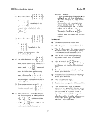
![Chapter 4: General Vector Spaces SSM: Elementary Linear Algebra
102
Section 4.8
Exercise Set 4.8
1. The reduced row echelon form of A is
6 4
7 7
17 2
7 7
1 0
0 1
0 0 0 0
,
⎡ ⎤
− −
⎢ ⎥
⎢ ⎥
⎢ ⎥
⎣ ⎦
so rank (A) = 2.
1 3 2
2 1 3
4 5 9
0 2 2
T
A
− −
⎡ ⎤
⎢ ⎥
= ⎢ ⎥
⎢ ⎥
⎢ ⎥
⎣ ⎦
and the reduced row
echelon form of T
A is
1 0 1
0 1 1
0 0 0
0 0 0
,
⎡ ⎤
⎢ ⎥
⎢ ⎥
⎢ ⎥
⎢ ⎥
⎣ ⎦
so
rank rank 2
( ) ( ) .
T
A A
= =
3. (a) Since rank (A) = 2, there are 2 leading
variables. Since nullity(A) = 3 − 2 = 1, there
is 1 parameter.
(b) Since rank(A) = 1, there is 1 leading
variable. Since nullity(A) = 3 − 1 = 2, there
are 2 parameters.
(c) Since rank(A) = 2, there are 2 leading
variables. Since nullity(A) = 4 − 2 = 2, there
are 2 parameters.
(d) Since rank(A) = 2, there are 2 leading
variables. Since nullity(A) = 5 − 2 = 3, there
are 3 parameters.
(e) Since rank(A) = 3, there are 3 leading
variables. Since nullity(A) = 5 − 3 = 2, there
are 2 parameters.
5. (a) Since A is 4 × 4, rank(A) + nullity(A) = 4,
and the largest possible value of rank(A) is
4, so the smallest possible value of
nullity(A) is 0.
(b) Since A is 3 × 5, rank(A) + nullity(A) = 5,
and the largest possible value of rank(A) is
3, so the smallest possible value of
nullity(A) is 2.
(c) Since A is 5 × 3, rank(A) + nullity(A) = 3,
and the largest possible value of rank(A) is
3, so the smallest possible value of
nullity(A) is 0.
7. (a) Since [ ]
rank( rank
) ,
A A
= b the system is
consistent, and since nullity(A) = 3 − 3 = 0,
there are 0 parameters in the general
solution.
(b) Since rank rank
( ) ,
A A
⎡ ⎤
⎣ ⎦
b the system is
inconsistent.
(c) Since rank rank
( ) ,
A A
⎡ ⎤
= ⎣ ⎦
b the system is
consistent, and since nullity(A) = 3 − 1 = 2,
there are 2 parameters in the general
solution.
(d) Since rank rank
( ) ,
A A
⎡ ⎤
= ⎣ ⎦
b the system is
consistent, and since nullity(A) = 9 − 2 = 7,
there are 7 parameters in the general
solution.
(e) Since rank rank
( ) ,
A A
⎡ ⎤
⎣ ⎦
b the system is
inconsistent.
(f) Since rank rank
( ,
A A
⎡ ⎤
= ⎣ ⎦
b the system is
consistent, and since nullity(A) = 4 − 0 = 4,
there are 4 parameters in the general
solution.
(g) Since rank rank
( ) ,
A A
⎡ ⎤
= ⎣ ⎦
b the system is
consistent, and since nullity(A) = 2 − 2 = 0,
there are 0 parameters in the general
solution.
9. The augmented matrix is
1
2
3
4
5
1 3
1 2
1 1
1 4
1 5
,
b
b
b
b
b
−
⎡ ⎤
⎢ ⎥
−
⎢ ⎥
⎢ ⎥
⎢ ⎥
−
⎢ ⎥
⎣ ⎦
which is
row equivalent to
2 1
2 1
3 2 1
4 2 1
5 2 1
1 0 3 2
0 1
0 0 4 3
0 0 2
0 0 8 7
.
b b
b b
b b b
b b b
b b b
−
⎡ ⎤
⎢ ⎥
−
⎢ ⎥
− +
⎢ ⎥
⎢ ⎥
+ −
⎢ ⎥
− +
⎣ ⎦
Thus,
the system is consistent if and only if
1 2 3
1 2 4
1 2 5
3 4 0
2 0
7 8 0
b b b
b b b
b b b
− + =
− + + =
− + =
which has the general solution 1 ,
b r
= 2 ,
b s
=
3 3 4 ,
b r s
= − + 4 2 ,
b r s
= − 5 7 8 .
b r s
= − +](https://image.slidesharecdn.com/elementary-linear-algebra-chapter1-220420115526/85/Elementary-linear-algebra-chapter-1-pdf-157-320.jpg)
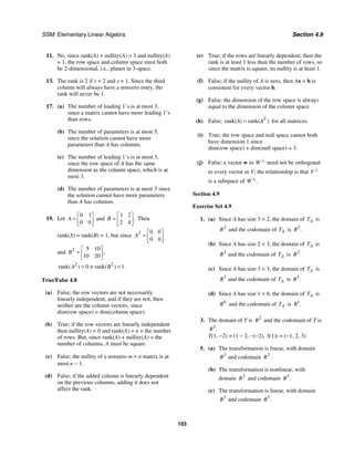
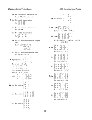
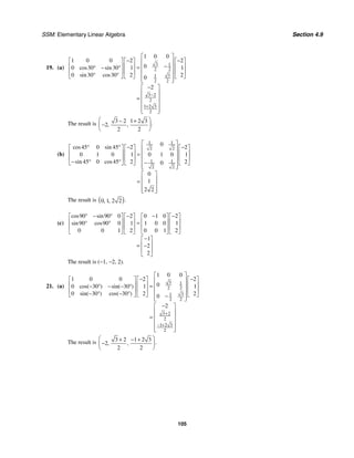
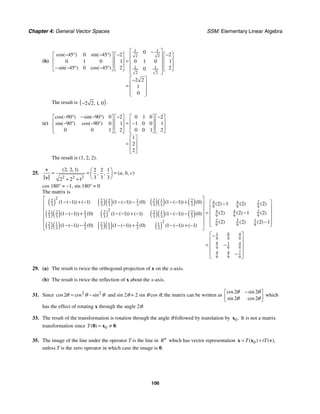
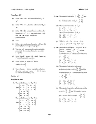
![Chapter 4: General Vector Spaces SSM: Elementary Linear Algebra
108
7. (a) The standard matrix for reflection about the yz-plane is
1 0 0
0 1 0
0 0 1
−
⎡ ⎤
⎢ ⎥
⎢ ⎥
⎣ ⎦
and the standard matrix for orthogonal
projection on the xz-plane is
1 0 0
0 0 0
0 0 1
.
⎡ ⎤
⎢ ⎥
⎢ ⎥
⎣ ⎦
1 0 0 1 0 0 1 0 0
0 0 0 0 1 0 0 0 0
0 0 1 0 0 1 0 0 1
− −
⎡ ⎤ ⎡ ⎤ ⎡ ⎤
⎢ ⎥ ⎢ ⎥ ⎢ ⎥
=
⎢ ⎥ ⎢ ⎥ ⎢ ⎥
⎣ ⎦ ⎣ ⎦ ⎣ ⎦
(b) The standard matrix for a rotation of 45° about the y-axis is
1 1
2 2
1 1
2 2
0
45 0 45
0 1 0 0 1 0
45 0 45 0
cos sin
sin cos
⎡ ⎤
° °
⎡ ⎤ ⎢ ⎥
⎢ ⎥ = ⎢ ⎥
⎢ ⎥ ⎢ ⎥
− ° ° −
⎣ ⎦ ⎢ ⎥
⎣ ⎦
and
the standard matrix for a dilation with factor 2
k = is
2 0 0
0 2 0
0 0 2
.
⎡ ⎤
⎢ ⎥
⎢ ⎥
⎢ ⎥
⎣ ⎦
1 1
2 2
1 1
2 2
0
2 0 0 1 0 1
0 1 0
0 2 0 0 2 0
1 0 1
0
0 0 2
⎡ ⎤
⎡ ⎤ ⎡ ⎤
⎢ ⎥
⎢ ⎥ ⎢ ⎥
=
⎢ ⎥
⎢ ⎥ ⎢ ⎥
⎢ ⎥
⎢ ⎥ −
⎢ ⎥
− ⎣ ⎦
⎣ ⎦ ⎢ ⎥
⎣ ⎦
(c) The standard matrix for orthogonal projection on the xy-plane is
1 0 0
0 1 0
0 0 0
⎡ ⎤
⎢ ⎥
⎢ ⎥
⎣ ⎦
and the standard matrix for
reflection about the yz-plane is
1 0 0
0 1 0
0 0 1
.
−
⎡ ⎤
⎢ ⎥
⎢ ⎥
⎣ ⎦
1 0 0 1 0 0 1 0 0
0 1 0 0 1 0 0 1 0
0 0 1 0 0 0 0 0 0
− −
⎡ ⎤ ⎡ ⎤ ⎡ ⎤
⎢ ⎥ ⎢ ⎥ ⎢ ⎥
=
⎢ ⎥ ⎢ ⎥ ⎢ ⎥
⎣ ⎦ ⎣ ⎦ ⎣ ⎦
9. (a) 1
1 0
0 0
[ ]
T
⎡ ⎤
= ⎢ ⎥
⎣ ⎦
and 2
0 0
0 1
[ ] .
T
⎡ ⎤
= ⎢ ⎥
⎣ ⎦
1 2 2 1
0 0
0 0
[ ][ ] [ ][ ]
T T T T
⎡ ⎤
= = ⎢ ⎥
⎣ ⎦
so 1 2 2 1.
T T T T
=](https://image.slidesharecdn.com/elementary-linear-algebra-chapter1-220420115526/85/Elementary-linear-algebra-chapter-1-pdf-163-320.jpg)
![SSM: Elementary Linear Algebra Section 4.10
109
(b) From Example 1, 1 2 1 2
2 1
1 2 1 2
cos( ) sin( )
[ ]
sin( ) cos( )
T T
θ θ θ θ
θ θ θ θ
+ − +
⎡ ⎤
= ⎢ ⎥
+ +
⎣ ⎦
1 2 1 2
1 1 2 2
1 1 2 2
1 2 1 2 1 2 1 2
1 2 1 2 1 2 1 2
1 2 1 2
1 2
[ ] [ ][ ]
cos sin cos sin
sin cos sin cos
cos cos sin sin cos sin sin cos
sin cos cos sin sin sin cos cos
cos( ) sin( )
sin( ) cos(
T T T T
θ θ θ θ
θ θ θ θ
θ θ θ θ θ θ θ θ
θ θ θ θ θ θ θ θ
θ θ θ θ
θ θ
=
− −
⎡ ⎤ ⎡ ⎤
= ⎢ ⎥ ⎢ ⎥
⎣ ⎦ ⎣ ⎦
− − −
⎡ ⎤
= ⎢ ⎥
+ − +
⎣ ⎦
+ − +
=
+ 1 2
2 1
)
[ ]
T T
θ θ
⎡ ⎤
⎢ ⎥
+
⎣ ⎦
=
Thus 1 2 2 1.
T T T T
=
(c) 1
1 0
0 0
[ ]
T
⎡ ⎤
= ⎢ ⎥
⎣ ⎦
and 2
cos sin
[ ] .
sin cos
T
θ θ
θ θ
−
⎡ ⎤
= ⎢ ⎥
⎣ ⎦
1 2
1 0
0 0
0 0
cos sin
[ ][ ]
sin cos
cos sin
T T
θ θ
θ θ
θ θ
−
⎡ ⎤ ⎡ ⎤
= ⎢ ⎥ ⎢ ⎥
⎣ ⎦ ⎣ ⎦
−
⎡ ⎤
= ⎢ ⎥
⎣ ⎦
2 1
1 0
0 0
0
0
cos sin
[ ][ ]
sin cos
cos
sin
T T
θ θ
θ θ
θ
θ
−
⎡ ⎤ ⎡ ⎤
= ⎢ ⎥ ⎢ ⎥
⎣ ⎦ ⎣ ⎦
⎡ ⎤
= ⎢ ⎥
⎣ ⎦
1 2 2 1
T T T T
≠
11. (a) Not one-to-one because the second row (column) is all 0’s, so the determinant is 0.
(b) One-to-one because the determinant is −1.
(c) One-to-one because the determinant is −1.
(d) One-to-one because the determinant is 2
0.
k ≠
(e) One-to-one because the determinant is 1.
(f) One-to-one because the determinant is −1.
(g) One-to-one because the determinant is 3
0.
k ≠
13. (a)
1 2
1 1
[ ]
T
⎡ ⎤
= ⎢ ⎥
−
⎣ ⎦
det[T] = 1 + 2 = 3 ≠ 0, so T is one-to-one.
1 2
1 3 3
1 1
3 3
1 1 2
1 1
3
[ ]
T −
⎡ ⎤
−
−
⎡ ⎤ ⎢ ⎥
= =
⎢ ⎥
⎣ ⎦ ⎢ ⎥
⎣ ⎦
1
1 2 1 2 1 2
1 2 1 1
3 3 3 3
( , ) ,
T w w w w w w
− ⎛ ⎞
= − +
⎜ ⎟
⎝ ⎠](https://image.slidesharecdn.com/elementary-linear-algebra-chapter1-220420115526/85/Elementary-linear-algebra-chapter-1-pdf-164-320.jpg)
![Chapter 4: General Vector Spaces SSM: Elementary Linear Algebra
110
(b)
4 6
2 3
[ ]
T
−
⎡ ⎤
= ⎢ ⎥
−
⎣ ⎦
det[T] = 12 − 12 = 0, so T is not one-to-one.
(c)
0 1
1 0
[ ]
T
−
⎡ ⎤
= ⎢ ⎥
−
⎣ ⎦
det[T] = 0 − 1 = −1 ≠ 0, so T is one-to-one.
1 1 0 1 0 1
1 0 1 0
1
[ ]
T − −
⎡ ⎤ ⎡ ⎤
= =
⎢ ⎥ ⎢ ⎥
−
− ⎣ ⎦ ⎣ ⎦
1
1 2 2 1
( , ) ( , )
T w w w w
−
= − −
(d)
3 0
5 0
[ ]
T
⎡ ⎤
= ⎢ ⎥
−
⎣ ⎦
det[T] = 3(0) − (−5)(0) = 0, so T is not one-to-one.
15. (a) The inverse is (another) reflection about the x-axis in 2
.
R
(b) The inverse is rotation through the angle
4
π
− in 2
.
R
(c) The inverse is contraction by a factor of
1
3
in 2
.
R
(d) The inverse is (another) reflection about the yz-plane in 3
.
R
(e) The inverse is dilation by a factor of 5 in 3
.
R
17. Let 1 1
( , ),
x y
=
u 2 2
( , ),
x y
=
v and k be a scalar.
(a) 1 2 1 2
1 2 1 2 1 2 1 2
1 1 2 2 1 1 2 2
2
2 2
( ) ( , )
( ( ) ( ), ( ) ( ))
(( ) ( ), ( ) ( ))
( ) ( )
T T x x y y
x x y y x x y y
x y x y x y x y
T T
+ = + +
= + + + + − +
= + + + − + −
= +
u v
u v
1 1
1 1 1 1
1 1 1 1
2
2
( ) ( , )
( , )
( , )
( )
T k T kx ky
kx ky kx ky
k x y x y
kT
=
= + −
= + −
=
u
u
T is a matrix operator.
(b) 1 1
1 1
1 1
1
1
( ) ( , )
( , )
( , )
T k T kx ky
kx ky
k x y
=
= +
≠ +
u
T is not a matrix operator, which can also be shown by considering T(u + v).](https://image.slidesharecdn.com/elementary-linear-algebra-chapter1-220420115526/85/Elementary-linear-algebra-chapter-1-pdf-165-320.jpg)
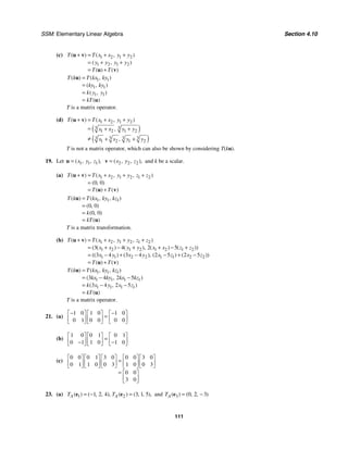
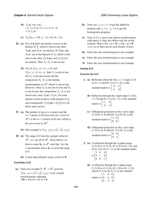
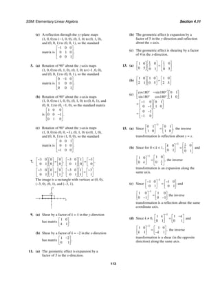
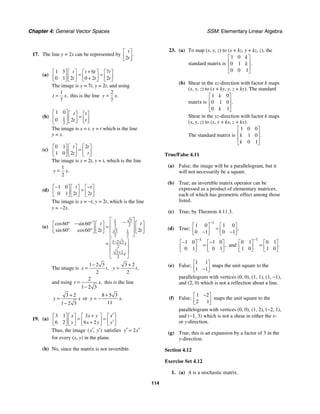
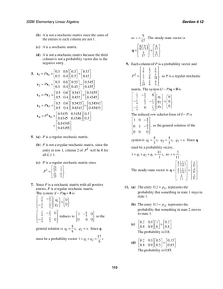
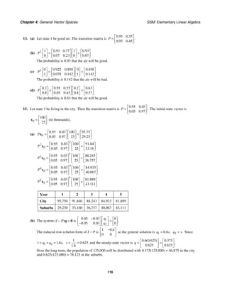
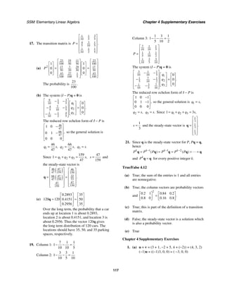
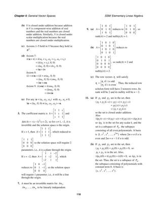
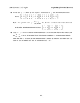
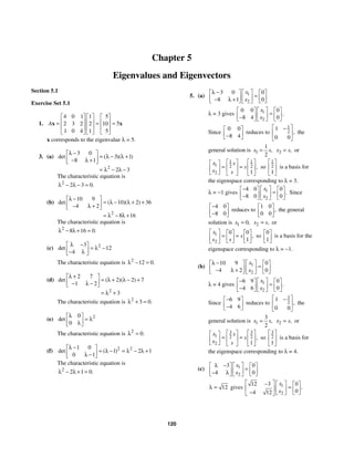
![SSM: Elementary Linear Algebra Section 5.1
121
Since
12 3
4 12
⎡ ⎤
−
⎢ ⎥
−
⎣ ⎦
reduces to
3
12
1
0 0
,
⎡ ⎤
−
⎢ ⎥
⎢ ⎥
⎣ ⎦
the general solution is 1
3
12
,
x s
= 2 ,
x s
=
or
3 3
1 12 12
2 1
,
s
x
s
x s
⎡ ⎤ ⎡ ⎤
⎡ ⎤
= =
⎢ ⎥ ⎢ ⎥
⎢ ⎥
⎣ ⎦ ⎢ ⎥ ⎢ ⎥
⎣ ⎦ ⎣ ⎦
so
3
12
1
⎡ ⎤
⎢ ⎥
⎢ ⎥
⎣ ⎦
is a
basis for the eigenspace corresponding to
12.
λ =
12
λ = − gives
1
2
12 3 0
0
4 12
.
x
x
⎡ ⎤
− − ⎡ ⎤ ⎡ ⎤
=
⎢ ⎥ ⎢ ⎥ ⎢ ⎥
− − ⎣ ⎦
⎣ ⎦
⎣ ⎦
Since
12 3
4 12
⎡ ⎤
− −
⎢ ⎥
− −
⎣ ⎦
reduces to
3
12
1
0 0
,
⎡ ⎤
⎢ ⎥
⎢ ⎥
⎣ ⎦
the general solution is
1
3
12
,
x s
= − 2 ,
x s
= or
3 3
1 12 12
2 1
,
s
x
s
x s
⎡ ⎤ ⎡ ⎤
− −
⎡ ⎤
= =
⎢ ⎥ ⎢ ⎥
⎢ ⎥
⎣ ⎦ ⎢ ⎥ ⎢ ⎥
⎣ ⎦ ⎣ ⎦
so
3
12
1
⎡ ⎤
−
⎢ ⎥
⎢ ⎥
⎣ ⎦
is
a basis for the eigenspace corresponding to
12.
λ = −
(d) There are no eigenspaces since there are no
real eigenvalues.
(e) 1
2
0 0
0 0
x
x
λ ⎡ ⎤
⎡ ⎤ ⎡ ⎤
=
⎢ ⎥
⎢ ⎥ ⎢ ⎥
λ
⎣ ⎦ ⎣ ⎦
⎣ ⎦
λ = 0 gives 1
2
0 0 0
0 0 0
.
x
x
⎡ ⎤
⎡ ⎤ ⎡ ⎤
=
⎢ ⎥
⎢ ⎥ ⎢ ⎥
⎣ ⎦ ⎣ ⎦
⎣ ⎦
Clearly, every vector in 2
R is a solution, so
1
0
,
⎡ ⎤
⎢ ⎥
⎣ ⎦
0
1
⎡ ⎤
⎢ ⎥
⎣ ⎦
is a basis for the eigenspace
corresponding to λ = 0.
(f) 1
2
1 0 0
0 1 0
x
x
λ − ⎡ ⎤
⎡ ⎤ ⎡ ⎤
=
⎢ ⎥
⎢ ⎥ ⎢ ⎥
λ −
⎣ ⎦ ⎣ ⎦
⎣ ⎦
λ = 1 gives 1
2
0 0 0
0 0 0
.
x
x
⎡ ⎤
⎡ ⎤ ⎡ ⎤
=
⎢ ⎥
⎢ ⎥ ⎢ ⎥
⎣ ⎦ ⎣ ⎦
⎣ ⎦
Clearly, every vector in 2
R is a solution, so
1
0
,
⎡ ⎤
⎢ ⎥
⎣ ⎦
0
1
⎡ ⎤
⎢ ⎥
⎣ ⎦
is a basis for the eigenspace
corresponding to λ = 1.
7. (a) The eigenvalues satisfy
3 2
6 11 6 0
λ − λ + λ − = or
(λ − 1)(λ − 2)(λ − 3) = 0, so the eigenvalues
are λ = 1, 2, 3.
(b) The eigenvalues satisfy 3
2 0
λ − λ = or
( )( )
2 2 0,
λ λ + λ − = so the eigenvalues
are 0 2 2
, , .
λ = −
(c) The eigenvalues satisfy 3 2
8 8 0
λ + λ + λ + =
or 2
8 1 0
( )( ) ,
λ + λ + = so the only (real)
eigenvalue is λ = −8.
(d) The eigenvalues satisfy 3 2
2 0
λ − λ − λ − =
or 2
2 1 0
( )( ) ,
λ − λ + λ + = so the only (real
eigenvalue is λ = 2.
(e) The eigenvalues satisfy
3 2
6 12 8 0
λ − λ + λ − = or 3
2 0
( ) ,
λ − = so
the only eigenvalue is λ = 2.
(f) The eigenvalues satisfy
3 2
2 15 36 0
λ − λ − λ + = or
2
4 3 0
( )( ) ,
λ + λ − = so the eigenvalues are
λ = −4, 3.
9. (a)
0 2 0
1 1 0
0 1 2 0
0 0 0 1
det
λ −
⎡ ⎤
⎢ ⎥
− λ −
⎢ ⎥
− λ +
⎢ ⎥
λ −
⎢ ⎥
⎣ ⎦
3 2
4 3 2
0 2
1 1 1
0 1 2
1 2 1 2 1 0
1 2 2
3 2
( )det
( ){ [ ( ) ] ( )}
( )( )
λ −
⎡ ⎤
⎢ ⎥
= λ − − λ −
⎢ ⎥
− λ +
⎣ ⎦
= λ − λ λ λ + − − −
= λ − λ + λ − λ −
= λ + λ − λ − λ +
The characteristic equation is
4 3 2
3 2 0.
λ + λ − λ − λ + =](https://image.slidesharecdn.com/elementary-linear-algebra-chapter1-220420115526/85/Elementary-linear-algebra-chapter-1-pdf-176-320.jpg)
![Chapter 5: Eigenvalues and Eigenvectors SSM: Elementary Linear Algebra
122
(b)
10 9 0 0
4 2 0 0
0 0 2 7
0 0 1 2
det
λ −
⎡ ⎤
⎢ ⎥
− λ +
⎢ ⎥
λ +
⎢ ⎥
− λ −
⎢ ⎥
⎣ ⎦
2 2
2 2
4 3 2
2 0 0 4 0 0
10 9
0 2 7 0 2 7
0 1 2 0 1 2
10 2 2 2 7 9 4 2 2 7
8 20 36 4 7
8 16 3
8 19 24 48
( )det det
( )( )[( )( ) ] ( )[( )( ) ]
( )( )
( )( )
λ + −
⎡ ⎤ ⎡ ⎤
⎢ ⎥ ⎢ ⎥
= λ − −
λ + λ +
⎢ ⎥ ⎢ ⎥
− λ − − λ −
⎣ ⎦ ⎣ ⎦
= λ − λ + λ + λ − + − − λ + λ − +
= λ − λ − + λ − +
= λ − λ + λ +
= λ − λ + λ − λ +
The characteristic equation is 4 3 2
8 19 24 48 0.
λ − λ + λ − λ + =
11. (a)
1
2
3
4
0 2 0 0
1 1 0 0
0 1 2 0 0
0 0 0 1 0
x
x
x
x
⎡ ⎤
λ −
⎡ ⎤ ⎡ ⎤
⎢ ⎥
⎢ ⎥ ⎢ ⎥
− λ −
⎢ ⎥ =
⎢ ⎥ ⎢ ⎥
− λ + ⎢ ⎥
⎢ ⎥ ⎢ ⎥
⎢ ⎥
λ −
⎢ ⎥ ⎢ ⎥
⎣ ⎦ ⎣ ⎦
⎣ ⎦
λ = 1 gives
1
2
3
4
1 0 2 0 0
1 1 1 0 0
0 1 3 0 0
0 0 0 0 0
.
x
x
x
x
⎡ ⎤
−
⎡ ⎤ ⎡ ⎤
⎢ ⎥
⎢ ⎥ ⎢ ⎥
− −
⎢ ⎥ =
⎢ ⎥ ⎢ ⎥
− ⎢ ⎥
⎢ ⎥ ⎢ ⎥
⎢ ⎥
⎢ ⎥ ⎢ ⎥
⎣ ⎦ ⎣ ⎦
⎣ ⎦
Since
1 0 2 0
1 1 1 0
0 1 3 0
0 0 0 0
−
⎡ ⎤
⎢ ⎥
− −
⎢ ⎥
−
⎢ ⎥
⎢ ⎥
⎣ ⎦
reduces to
1 0 2 0
0 1 3 0
0 0 0 0
0 0 0 0
,
−
⎡ ⎤
⎢ ⎥
−
⎢ ⎥
⎢ ⎥
⎢ ⎥
⎣ ⎦
the general solution is 1 2 ,
x s
= 2 3 ,
x s
= 3 ,
x s
=
4
x t
= or
1
2
3
4
2 2 0
3 3 0
1 0
0 1
,
x s
x s
s t
x s
t
x
⎡ ⎤ ⎡ ⎤ ⎡ ⎤ ⎡ ⎤
⎢ ⎥ ⎢ ⎥ ⎢ ⎥ ⎢ ⎥
⎢ ⎥ = = +
⎢ ⎥ ⎢ ⎥ ⎢ ⎥
⎢ ⎥ ⎢ ⎥ ⎢ ⎥ ⎢ ⎥
⎢ ⎥ ⎢ ⎥ ⎢ ⎥ ⎢ ⎥
⎣ ⎦ ⎣ ⎦ ⎣ ⎦
⎣ ⎦
so
2
3
1
0
,
⎡ ⎤
⎢ ⎥
⎢ ⎥
⎢ ⎥
⎢ ⎥
⎣ ⎦
0
0
0
1
⎡ ⎤
⎢ ⎥
⎢ ⎥
⎢ ⎥
⎢ ⎥
⎣ ⎦
is a basis for the eigenspace corresponding to λ = 1.
λ = −2 gives
1
2
3
4
2 0 2 0 0
1 2 1 0 0
0 1 0 0 0
0 0 0 3 0
.
x
x
x
x
⎡ ⎤
− −
⎡ ⎤ ⎡ ⎤
⎢ ⎥
⎢ ⎥ ⎢ ⎥
− − −
⎢ ⎥ =
⎢ ⎥ ⎢ ⎥
− ⎢ ⎥
⎢ ⎥ ⎢ ⎥
⎢ ⎥
−
⎢ ⎥ ⎢ ⎥
⎣ ⎦ ⎣ ⎦
⎣ ⎦
Since
2 0 2 0
1 2 1 0
0 1 0 0
0 0 0 3
− −
⎡ ⎤
⎢ ⎥
− − −
⎢ ⎥
−
⎢ ⎥
−
⎢ ⎥
⎣ ⎦
reduces to
1 0 1 0
0 1 0 0
0 0 0 1
0 0 0 0
,
⎡ ⎤
⎢ ⎥
⎢ ⎥
⎢ ⎥
⎢ ⎥
⎣ ⎦
the general solution is 1 ,
x s
= − 2 0,
x = 3 ,
x s
=
4 0
x = or
1
2
3
4
1
0 0
1
0 0
,
x s
x
s
x s
x
⎡ ⎤ − −
⎡ ⎤ ⎡ ⎤
⎢ ⎥ ⎢ ⎥ ⎢ ⎥
⎢ ⎥ = =
⎢ ⎥ ⎢ ⎥
⎢ ⎥ ⎢ ⎥ ⎢ ⎥
⎢ ⎥ ⎢ ⎥ ⎢ ⎥
⎣ ⎦ ⎣ ⎦
⎣ ⎦
so
1
0
1
0
−
⎡ ⎤
⎢ ⎥
⎢ ⎥
⎢ ⎥
⎢ ⎥
⎣ ⎦
is a basis for the eigenspace corresponding to λ = −2.
λ = −1 gives
1
2
3
4
1 0 2 0 0
1 1 1 0 0
0 1 1 0 0
0 0 0 2 0
.
x
x
x
x
⎡ ⎤
− −
⎡ ⎤ ⎡ ⎤
⎢ ⎥
⎢ ⎥ ⎢ ⎥
− − −
⎢ ⎥ =
⎢ ⎥ ⎢ ⎥
− ⎢ ⎥
⎢ ⎥ ⎢ ⎥
⎢ ⎥
−
⎢ ⎥ ⎢ ⎥
⎣ ⎦ ⎣ ⎦
⎣ ⎦](https://image.slidesharecdn.com/elementary-linear-algebra-chapter1-220420115526/85/Elementary-linear-algebra-chapter-1-pdf-177-320.jpg)
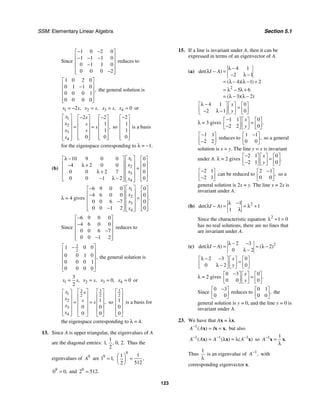
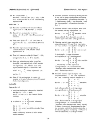
![SSM: Elementary Linear Algebra Section 5.2
125
13. A has eigenvalues 1 1
λ = and 2 1
λ = − (the
diagonal entries, since A is triangular).
(λI − A)x = 0 is 1
2
1 0 0
6 1 0
.
x
x
λ − ⎡ ⎤
⎡ ⎤ ⎡ ⎤
=
⎢ ⎥
⎢ ⎥ ⎢ ⎥
− λ +
⎣ ⎦ ⎣ ⎦
⎣ ⎦
1 1
λ = gives 1
2
0 0 0
6 2 0
.
x
x
⎡ ⎤
⎡ ⎤ ⎡ ⎤
=
⎢ ⎥
⎢ ⎥ ⎢ ⎥
−
⎣ ⎦ ⎣ ⎦
⎣ ⎦
Since
0 0
6 2
⎡ ⎤
⎢ ⎥
−
⎣ ⎦
reduces to
1
3
1
0 0
,
⎡ ⎤
−
⎢ ⎥
⎣ ⎦
the general
solution is 1
1
3
,
x s
= 2 ,
x s
= or
1
1 3
2 1
,
x
s
x
⎡ ⎤
⎡ ⎤
= ⎢ ⎥
⎢ ⎥
⎣ ⎦ ⎣ ⎦
and
1
3
1
1
⎡ ⎤
= ⎢ ⎥
⎣ ⎦
p is a basis for the eigenspace
corresponding to 1 1.
λ =
2 1
λ = − gives 1
2
2 0 0
6 0 0
.
x
x
− ⎡ ⎤
⎡ ⎤ ⎡ ⎤
=
⎢ ⎥
⎢ ⎥ ⎢ ⎥
−
⎣ ⎦ ⎣ ⎦
⎣ ⎦
Since
2 0
6 0
−
⎡ ⎤
⎢ ⎥
−
⎣ ⎦
reduces to
1 0
0 0
,
⎡ ⎤
⎢ ⎥
⎣ ⎦
the general
solution is 1 0,
x = 2
x s
= or 1
2
0
1
,
x
s
x
⎡ ⎤ ⎡ ⎤
=
⎢ ⎥ ⎢ ⎥
⎣ ⎦
⎣ ⎦
and
2
0
1
⎡ ⎤
= ⎢ ⎥
⎣ ⎦
p is a basis for the eigenspace
corresponding to 2 1.
λ = −
Thus,
1
3
1 2
0
1 1
[ ]
P
⎡ ⎤
= = ⎢ ⎥
⎣ ⎦
p p diagonalizes A.
1
1 3
1
2
0
3 0 1 0
3 1 6 1 1 1
0
0
1 0
0 1
P AP
− ⎡ ⎤
⎡ ⎤ ⎡ ⎤
= ⎢ ⎥
⎢ ⎥ ⎢ ⎥
− −
⎣ ⎦ ⎣ ⎦ ⎣ ⎦
λ
⎡ ⎤
= ⎢ ⎥
λ
⎣ ⎦
⎡ ⎤
= ⎢ ⎥
−
⎣ ⎦
15. A has eigenvalues 1 2
λ = and 2 3
λ = (the
diagonal entries, since A is triangular).
( )
I A
λ − =
x 0 is
1
2
3
2 0 2 0
0 3 0 0
0 0 3 0
.
x
x
x
⎡ ⎤
λ −
⎡ ⎤ ⎡ ⎤
⎢ ⎥
⎢ ⎥ ⎢ ⎥
=
λ −
⎢ ⎥
⎢ ⎥ ⎢ ⎥
λ −
⎣ ⎦ ⎣ ⎦
⎣ ⎦
1 2
λ = gives
1
2
3
0 0 2 0
0 1 0 0
0 0 1 0
.
x
x
x
⎡ ⎤
⎡ ⎤ ⎡ ⎤
⎢ ⎥
⎢ ⎥ ⎢ ⎥
=
−
⎢ ⎥
⎢ ⎥ ⎢ ⎥
−
⎣ ⎦ ⎣ ⎦
⎣ ⎦
Since
0 0 2
0 1 0
0 0 1
⎡ ⎤
⎢ ⎥
−
⎢ ⎥
−
⎣ ⎦
reduces to
0 1 0
0 0 1
0 0 0
,
⎡ ⎤
⎢ ⎥
⎢ ⎥
⎣ ⎦
the
general solution is 1 ,
x s
= 2 0,
x = 3 0
x = or
1
2
3
1
0
0
x
x s
x
⎡ ⎤ ⎡ ⎤
⎢ ⎥ ⎢ ⎥
=
⎢ ⎥ ⎢ ⎥
⎣ ⎦
⎣ ⎦
and 1
1
0
0
⎡ ⎤
⎢ ⎥
=
⎢ ⎥
⎣ ⎦
p is a basis for the
eigenspace corresponding to 1 2.
λ =
2 3
λ = gives
1
2
3
1 0 2 0
0 0 0 0
0 0 0 0
x
x
x
⎡ ⎤
⎡ ⎤ ⎡ ⎤
⎢ ⎥
⎢ ⎥ ⎢ ⎥
=
⎢ ⎥
⎢ ⎥ ⎢ ⎥
⎣ ⎦ ⎣ ⎦
⎣ ⎦
which has
general solution 1 2 ,
x s
= − 2 ,
x t
= 3 ,
x s
= or
1
2
3
2 0
0 1
1 0
,
x
x s t
x
⎡ ⎤ −
⎡ ⎤ ⎡ ⎤
⎢ ⎥ ⎢ ⎥ ⎢ ⎥
= +
⎢ ⎥ ⎢ ⎥ ⎢ ⎥
⎣ ⎦ ⎣ ⎦
⎣ ⎦
and 2
2
0
1
,
−
⎡ ⎤
⎢ ⎥
=
⎢ ⎥
⎣ ⎦
p 3
0
1
0
⎡ ⎤
⎢ ⎥
=
⎢ ⎥
⎣ ⎦
p
is a basis for the eigenspace corresponding to
2 3.
λ = Thus 1 2 3
1 2 0
0 0 1
0 1 0
[ ]
P
−
⎡ ⎤
⎢ ⎥
= =
⎢ ⎥
⎣ ⎦
p p p
diagonalizes A.
1
1
2
2
1 0 2 2 0 2 1 2 0
0 0 1 0 3 0 0 0 1
0 1 0 0 0 3 0 1 0
0 0
0 0
0 0
2 0 0
0 3 0
0 0 3
P AP
−
− −
⎡ ⎤ ⎡ ⎤ ⎡ ⎤
⎢ ⎥ ⎢ ⎥ ⎢ ⎥
=
⎢ ⎥ ⎢ ⎥ ⎢ ⎥
⎣ ⎦ ⎣ ⎦ ⎣ ⎦
λ
⎡ ⎤
⎢ ⎥
= λ
⎢ ⎥
λ
⎣ ⎦
⎡ ⎤
⎢ ⎥
=
⎢ ⎥
⎣ ⎦
17.
3 2
1 4 2
3 4 0
3 1 3
6 11 6
1 2 3
det( )
( )( )( )
I A
x x x
x x x
λ + −
λ − = λ −
− λ −
= − + −
= − − −
The eigenvalues are 1 1,
λ = 2 2,
λ = and 3 3,
λ =
each with algebraic multiplicity 1. Since each
eigenvalue must have nonzero geometric
multiplicity, the geometric multiplicity of each
eigenvalue is also 1 and A is diagonalizable.
( )
I A
λ − =
x 0 is
1
2
3
1 4 2 0
3 4 0 0
3 1 3 0
.
x
x
x
⎡ ⎤
λ + −
⎡ ⎤ ⎡ ⎤
⎢ ⎥
⎢ ⎥ ⎢ ⎥
=
λ −
⎢ ⎥
⎢ ⎥ ⎢ ⎥
− λ −
⎣ ⎦ ⎣ ⎦
⎣ ⎦](https://image.slidesharecdn.com/elementary-linear-algebra-chapter1-220420115526/85/Elementary-linear-algebra-chapter-1-pdf-180-320.jpg)
![Chapter 5: Eigenvalues and Eigenvectors SSM: Elementary Linear Algebra
126
1 1
λ = gives
1
2
3
2 4 2 0
3 3 0 0
3 1 2 0
.
x
x
x
⎡ ⎤
−
⎡ ⎤ ⎡ ⎤
⎢ ⎥
⎢ ⎥ ⎢ ⎥
=
−
⎢ ⎥
⎢ ⎥ ⎢ ⎥
− −
⎣ ⎦ ⎣ ⎦
⎣ ⎦
Since
2 4 2
3 3 0
3 1 2
−
⎡ ⎤
⎢ ⎥
−
⎢ ⎥
− −
⎣ ⎦
reduces to
1 0 1
0 1 1
0 0 0
,
−
⎡ ⎤
⎢ ⎥
−
⎢ ⎥
⎣ ⎦
the
general solution is 1 ,
x s
= 2 ,
x s
= 3 ,
x s
= or
1
2
3
1
1
1
x
x s
x
⎡ ⎤ ⎡ ⎤
⎢ ⎥ ⎢ ⎥
=
⎢ ⎥ ⎢ ⎥
⎣ ⎦
⎣ ⎦
and 1
1
1
1
⎡ ⎤
⎢ ⎥
=
⎢ ⎥
⎣ ⎦
p is a basis for the
eigenspace corresponding to 1 1.
λ =
2 2
λ = gives
1
2
3
3 4 2 0
3 2 0 0
3 1 1 0
.
x
x
x
⎡ ⎤
−
⎡ ⎤ ⎡ ⎤
⎢ ⎥
⎢ ⎥ ⎢ ⎥
=
−
⎢ ⎥
⎢ ⎥ ⎢ ⎥
− −
⎣ ⎦ ⎣ ⎦
⎣ ⎦
Since
3 4 2
3 2 0
3 1 1
−
⎡ ⎤
⎢ ⎥
−
⎢ ⎥
− −
⎣ ⎦
reduces to
2
3
1 0
0 1 1
0 0 0
,
⎡ ⎤
−
⎢ ⎥
−
⎢ ⎥
⎢ ⎥
⎣ ⎦
the general solution is 1
2
3
,
x s
= 2 ,
x s
= 3
x s
=
or 1 2 ,
x t
= 2 3 ,
x t
= 3 3
x t
= which is
1
2
3
2
3
3
x
x t
x
⎡ ⎤ ⎡ ⎤
⎢ ⎥ ⎢ ⎥
=
⎢ ⎥ ⎢ ⎥
⎣ ⎦
⎣ ⎦
and 2
2
3
3
⎡ ⎤
⎢ ⎥
=
⎢ ⎥
⎣ ⎦
p is a basis for the
eigenspace corresponding to 2 2.
λ =
3 3
λ = gives
1
2
3
4 4 2 0
3 1 0 0
3 1 0 0
.
x
x
x
⎡ ⎤
−
⎡ ⎤ ⎡ ⎤
⎢ ⎥
⎢ ⎥ ⎢ ⎥
=
−
⎢ ⎥
⎢ ⎥ ⎢ ⎥
−
⎣ ⎦ ⎣ ⎦
⎣ ⎦
Since
4 4 2
3 1 0
3 1 0
−
⎡ ⎤
⎢ ⎥
−
⎢ ⎥
−
⎣ ⎦
reduces to
1
4
3
4
1 0
0 1
0 0 0
,
⎡ ⎤
−
⎢ ⎥
−
⎢ ⎥
⎢ ⎥
⎣ ⎦
a
general solution is 1
1
4
,
x s
= 2
3
4
,
x s
= 3
x s
= or
1 ,
x t
= 2 3 ,
x t
= 3 4
x t
= which is
1
2
3
1
3
4
x
x t
x
⎡ ⎤ ⎡ ⎤
⎢ ⎥ ⎢ ⎥
=
⎢ ⎥ ⎢ ⎥
⎣ ⎦
⎣ ⎦
and 3
1
3
4
⎡ ⎤
⎢ ⎥
=
⎢ ⎥
⎣ ⎦
p is a basis for the eigenspace
corresponding to 3 3.
λ =
Thus 1 2 3
1 2 1
1 3 3
1 3 4
[ ]
P
⎡ ⎤
⎢ ⎥
= =
⎢ ⎥
⎣ ⎦
p p p
diagonalizes A and
1
1
2
3
0 0 1 0 0
0 0 0 2 0
0 0 3
0 0
.
P AP
−
λ
⎡ ⎤ ⎡ ⎤
⎢ ⎥ ⎢ ⎥
λ
= =
⎢ ⎥ ⎢ ⎥
λ ⎣ ⎦
⎣ ⎦
19. Since A is triangular with diagonal entries of 0,
0, 1, the eigenvalues are 1 0
λ = (with algebraic
multiplicity 2) and 2 1.
λ =
2 1
λ = must also have geometric multiplicity 1.
( )
I A
λ − =
x 0 is
1
2
3
0 0 0
0 0 0
3 0 1 0
.
x
x
x
⎡ ⎤
λ
⎡ ⎤ ⎡ ⎤
⎢ ⎥
⎢ ⎥ ⎢ ⎥
=
λ
⎢ ⎥
⎢ ⎥ ⎢ ⎥
− λ −
⎣ ⎦ ⎣ ⎦
⎣ ⎦
1 0
λ = gives
1
2
3
0 0 0 0
0 0 0 0
3 0 1 0
.
x
x
x
⎡ ⎤
⎡ ⎤ ⎡ ⎤
⎢ ⎥
⎢ ⎥ ⎢ ⎥
=
⎢ ⎥
⎢ ⎥ ⎢ ⎥
− −
⎣ ⎦ ⎣ ⎦
⎣ ⎦
Since
0 0 0
0 0 0
3 0 1
⎡ ⎤
⎢ ⎥
⎢ ⎥
− −
⎣ ⎦
reduces to
1
3
1 0
0 0 0
0 0 0
,
⎡ ⎤
⎢ ⎥
⎢ ⎥
⎢ ⎥
⎣ ⎦
a
general solution is 1
1
3
,
x r
= − 2 ,
x t
= 3
x r
= or
1 ,
x s
= 2 ,
x t
= 3 3
x s
= − which is
1
2
3
1 0
0 1
3 0
.
x
x s t
x
⎡ ⎤ ⎡ ⎤ ⎡ ⎤
⎢ ⎥ ⎢ ⎥ ⎢ ⎥
= +
⎢ ⎥ ⎢ ⎥ ⎢ ⎥
−
⎣ ⎦ ⎣ ⎦
⎣ ⎦
Thus 1 0
λ = has
geometric multiplicity 2, and A is diagonalizable.
1
1
0
3
,
⎡ ⎤
⎢ ⎥
=
⎢ ⎥
−
⎣ ⎦
p 2
0
1
0
⎡ ⎤
⎢ ⎥
=
⎢ ⎥
⎣ ⎦
p are a basis for the
eigenspace corresponding to 1 0.
λ =
2 1
λ = gives
1
2
3
1 0 0 0
0 1 0 0
3 0 0 0
.
x
x
x
⎡ ⎤
⎡ ⎤ ⎡ ⎤
⎢ ⎥
⎢ ⎥ ⎢ ⎥
=
⎢ ⎥
⎢ ⎥ ⎢ ⎥
−
⎣ ⎦ ⎣ ⎦
⎣ ⎦
Since
1 0 0
0 1 0
3 0 0
⎡ ⎤
⎢ ⎥
⎢ ⎥
−
⎣ ⎦
reduces to
1 0 0
0 1 0
0 0 0
,
⎡ ⎤
⎢ ⎥
⎢ ⎥
⎣ ⎦
a
general solution is 1 0,
x = 2 0,
x = 3
x s
= or
1
2
3
0
0
1
x
x s
x
⎡ ⎤ ⎡ ⎤
⎢ ⎥ ⎢ ⎥
=
⎢ ⎥ ⎢ ⎥
⎣ ⎦
⎣ ⎦
and 3
0
0
1
⎡ ⎤
⎢ ⎥
=
⎢ ⎥
⎣ ⎦
p is a basis for the
eigenspace corresponding to 2 1.
λ =
Thus 1 2 3
1 0 0
0 1 0
3 0 1
[ ]
P
⎡ ⎤
⎢ ⎥
= =
⎢ ⎥
−
⎣ ⎦
p p p](https://image.slidesharecdn.com/elementary-linear-algebra-chapter1-220420115526/85/Elementary-linear-algebra-chapter-1-pdf-181-320.jpg)
![SSM: Elementary Linear Algebra Section 5.2
127
diagonalizes A and
1
1
1
2
0 0 0 0 0
0 0 0 0 0
0 0 1
0 0
.
P AP
−
λ
⎡ ⎤ ⎡ ⎤
⎢ ⎥ ⎢ ⎥
= =
λ
⎢ ⎥ ⎢ ⎥
λ ⎣ ⎦
⎣ ⎦
21. Since A is triangular with entries −2, −2, 3, and 3
on the diagonal, the eigenvalues are 1 2
λ = − and
2 3,
λ = both with algebraic multiplicity 2.
( )
I A
λ − =
x 0 is
1
2
3
4
2 0 0 0 0
0 2 5 5 0
0 0 3 0 0
0 0 0 3 0
.
x
x
x
x
⎡ ⎤
λ +
⎡ ⎤ ⎡ ⎤
⎢ ⎥
⎢ ⎥ ⎢ ⎥
λ + −
⎢ ⎥ =
⎢ ⎥ ⎢ ⎥
λ − ⎢ ⎥
⎢ ⎥ ⎢ ⎥
⎢ ⎥
λ −
⎢ ⎥ ⎢ ⎥
⎣ ⎦ ⎣ ⎦
⎣ ⎦
1 2
λ = − gives
1
2
3
4
0 0 0 0 0
0 0 5 5 0
0 0 5 0 0
0 0 0 5 0
.
x
x
x
x
⎡ ⎤
⎡ ⎤ ⎡ ⎤
⎢ ⎥
⎢ ⎥ ⎢ ⎥
−
⎢ ⎥ =
⎢ ⎥ ⎢ ⎥
− ⎢ ⎥
⎢ ⎥ ⎢ ⎥
⎢ ⎥
−
⎢ ⎥ ⎢ ⎥
⎣ ⎦ ⎣ ⎦
⎣ ⎦
Since
0 0 0 0
0 0 5 5
0 0 5 0
0 0 0 5
⎡ ⎤
⎢ ⎥
−
⎢ ⎥
−
⎢ ⎥
−
⎢ ⎥
⎣ ⎦
reduces to
0 0 1 0
0 0 0 1
0 0 0 0
0 0 0 0
,
⎡ ⎤
⎢ ⎥
⎢ ⎥
⎢ ⎥
⎢ ⎥
⎣ ⎦
a general solution is 1 ,
x s
=
2 ,
x t
= 3 0,
x = 4 0
x = or
1
2
3
4
1 0
0 1
0 0
0 0
.
x
x
s t
x
x
⎡ ⎤ ⎡ ⎤ ⎡ ⎤
⎢ ⎥ ⎢ ⎥ ⎢ ⎥
⎢ ⎥ = +
⎢ ⎥ ⎢ ⎥
⎢ ⎥ ⎢ ⎥ ⎢ ⎥
⎢ ⎥ ⎢ ⎥ ⎢ ⎥
⎣ ⎦ ⎣ ⎦
⎣ ⎦
Thus 1 2
λ = − has geometric multiplicity 2, and
1
1
0
0
0
,
⎡ ⎤
⎢ ⎥
= ⎢ ⎥
⎢ ⎥
⎢ ⎥
⎣ ⎦
p 2
0
1
0
0
⎡ ⎤
⎢ ⎥
= ⎢ ⎥
⎢ ⎥
⎢ ⎥
⎣ ⎦
p are a basis for the
eigenspace corresponding to 1 2.
λ = −
2 3
λ = gives
1
2
3
4
5 0 0 0 0
0 5 5 5 0
0 0 0 0 0
0 0 0 0 0
.
x
x
x
x
⎡ ⎤
⎡ ⎤ ⎡ ⎤
⎢ ⎥
⎢ ⎥ ⎢ ⎥
−
⎢ ⎥ =
⎢ ⎥ ⎢ ⎥
⎢ ⎥
⎢ ⎥ ⎢ ⎥
⎢ ⎥
⎢ ⎥ ⎢ ⎥
⎣ ⎦ ⎣ ⎦
⎣ ⎦
Since
5 0 0 0
0 5 5 5
0 0 0 0
0 0 0 0
⎡ ⎤
⎢ ⎥
−
⎢ ⎥
⎢ ⎥
⎢ ⎥
⎣ ⎦
reduces to
1 0 0 0
0 1 1 1
0 0 0 0
0 0 0 0
,
⎡ ⎤
⎢ ⎥
−
⎢ ⎥
⎢ ⎥
⎢ ⎥
⎣ ⎦
a general solution is 1 0,
x =
2 ,
x s t
= − 3 ,
x s
= 4 ,
x t
= or
1
2
3
4
0 0
1 1
1 0
0 1
.
x
x
s t
x
x
⎡ ⎤ ⎡ ⎤ ⎡ ⎤
⎢ ⎥ ⎢ ⎥ ⎢ ⎥
−
⎢ ⎥ = +
⎢ ⎥ ⎢ ⎥
⎢ ⎥ ⎢ ⎥ ⎢ ⎥
⎢ ⎥ ⎢ ⎥ ⎢ ⎥
⎣ ⎦ ⎣ ⎦
⎣ ⎦
Thus 2 3
λ = has geometric multiplicity 2, and
3
0
1
1
0
,
⎡ ⎤
⎢ ⎥
= ⎢ ⎥
⎢ ⎥
⎢ ⎥
⎣ ⎦
p 4
0
1
0
1
⎡ ⎤
⎢ ⎥
−
= ⎢ ⎥
⎢ ⎥
⎢ ⎥
⎣ ⎦
p are a basis for the
eigenspace corresponding to 2 3.
λ =
Since the geometric and algebraic multiplicities
are equal for both eigenvalues, A is
diagonalizable.
1 2 3 4
1 0 0 0
0 1 1 1
0 0 1 0
0 0 0 1
[ ]
P
⎡ ⎤
⎢ ⎥
−
= = ⎢ ⎥
⎢ ⎥
⎢ ⎥
⎣ ⎦
p p p p
diagonalizes A, and
1
1 1
2
2
0 0 0
0 0 0
0 0 0
0 0 0
2 0 0 0
0 2 0 0
0 0 3 0
0 0 0 3
.
P AP
−
λ
⎡ ⎤
⎢ ⎥
λ
= ⎢ ⎥
λ
⎢ ⎥
⎢ ⎥
λ
⎣ ⎦
−
⎡ ⎤
⎢ ⎥
−
= ⎢ ⎥
⎢ ⎥
⎢ ⎥
⎣ ⎦
23.
3 2
1 7 1
0 1 0
0 15 2
2 2
2 1 1
det( )
( )( )( )
I A
λ + −
λ − = λ −
− λ +
= λ + λ − λ −
= λ + λ + λ −
Thus, the eigenvalues of A are 1 2,
λ = −
2 1,
λ = − and 3 1.
λ =
( )
I A
λ − =
x 0 is
1
2
3
1 7 1 0
0 1 0 0
0 15 2 0
.
x
x
x
⎡ ⎤
λ + −
⎡ ⎤ ⎡ ⎤
⎢ ⎥
⎢ ⎥ ⎢ ⎥
=
λ −
⎢ ⎥
⎢ ⎥ ⎢ ⎥
− λ +
⎣ ⎦ ⎣ ⎦
⎣ ⎦
1 2
λ = − gives
1
2
3
1 7 1 0
0 3 0 0
0 15 0 0
.
x
x
x
⎡ ⎤
− −
⎡ ⎤ ⎡ ⎤
⎢ ⎥
⎢ ⎥ ⎢ ⎥
=
−
⎢ ⎥
⎢ ⎥ ⎢ ⎥
−
⎣ ⎦ ⎣ ⎦
⎣ ⎦](https://image.slidesharecdn.com/elementary-linear-algebra-chapter1-220420115526/85/Elementary-linear-algebra-chapter-1-pdf-182-320.jpg)
![Chapter 5: Eigenvalues and Eigenvectors SSM: Elementary Linear Algebra
128
Since
1 7 1
0 3 0
0 15 0
− −
⎡ ⎤
⎢ ⎥
−
⎢ ⎥
−
⎣ ⎦
reduces to
1 0 1
0 1 0
0 0 0
,
−
⎡ ⎤
⎢ ⎥
⎢ ⎥
⎣ ⎦
a
general solution is 1 ,
x s
= 2 0,
x = 3 ,
x s
= or
1
2
3
1
0
1
,
x
x s
x
⎡ ⎤ ⎡ ⎤
⎢ ⎥ ⎢ ⎥
=
⎢ ⎥ ⎢ ⎥
⎣ ⎦
⎣ ⎦
so 1
1
0
1
⎡ ⎤
⎢ ⎥
=
⎢ ⎥
⎣ ⎦
p is a basis for the
eigenspace corresponding to 1 2.
λ = −
2 1
λ = − gives
1
2
3
0 7 1 0
0 2 0 0
0 15 1 0
.
x
x
x
⎡ ⎤
−
⎡ ⎤ ⎡ ⎤
⎢ ⎥
⎢ ⎥ ⎢ ⎥
=
−
⎢ ⎥
⎢ ⎥ ⎢ ⎥
−
⎣ ⎦ ⎣ ⎦
⎣ ⎦
Since
0 7 1
0 2 0
0 15 1
−
⎡ ⎤
⎢ ⎥
−
⎢ ⎥
−
⎣ ⎦
reduces to
0 1 0
0 0 1
0 0 0
,
⎡ ⎤
⎢ ⎥
⎢ ⎥
⎣ ⎦
a
general solution is 1 ,
x s
= 2 0,
x = 3 0,
x = or
1
2
3
1
0
0
x
x s
x
⎡ ⎤ ⎡ ⎤
⎢ ⎥ ⎢ ⎥
=
⎢ ⎥ ⎢ ⎥
⎣ ⎦
⎣ ⎦
so 2
1
0
0
⎡ ⎤
⎢ ⎥
=
⎢ ⎥
⎣ ⎦
p is a basis for the
eigenspace corresponding to 2 1.
λ = −
3 1
λ = gives
1
2
3
2 7 1 0
0 0 0 0
0 15 3 0
.
x
x
x
⎡ ⎤
−
⎡ ⎤ ⎡ ⎤
⎢ ⎥
⎢ ⎥ ⎢ ⎥
=
⎢ ⎥
⎢ ⎥ ⎢ ⎥
−
⎣ ⎦ ⎣ ⎦
⎣ ⎦
Since
2 7 1
0 0 0
0 15 3
−
⎡ ⎤
⎢ ⎥
⎢ ⎥
−
⎣ ⎦
reduces to
1
5
1
5
1 0
0 1
0 0 0
,
⎡ ⎤
−
⎢ ⎥
−
⎢ ⎥
⎢ ⎥
⎣ ⎦
a
general solution is 1
1
5
,
x s
= 2
1
5
,
x s
= 3
x s
= or
1 ,
x t
= 2 ,
x t
= 3 5
x t
= which is
1
2
3
1
1
5
x
x t
x
⎡ ⎤ ⎡ ⎤
⎢ ⎥ ⎢ ⎥
=
⎢ ⎥ ⎢ ⎥
⎣ ⎦
⎣ ⎦
so
3
1
1
5
⎡ ⎤
⎢ ⎥
=
⎢ ⎥
⎣ ⎦
p is a basis for the eigenspace
corresponding to 3 1.
λ =
1 2 3
1 1 1
0 0 1
1 0 5
[ ]
P
⎡ ⎤
⎢ ⎥
= =
⎢ ⎥
⎣ ⎦
p p p diagonalizes A,
and 1
1
2
3
0 5 1 1 7 1 1 1 1
1 4 1 0 1 0 0 0 1
0 1 0 0 15 2 1 0 5
0 0
0 0
0 0
2 0 0
0 1 0
0 0 1
D P AP
−
=
− − −
⎡ ⎤ ⎡ ⎤ ⎡ ⎤
⎢ ⎥ ⎢ ⎥ ⎢ ⎥
= −
⎢ ⎥ ⎢ ⎥ ⎢ ⎥
−
⎣ ⎦ ⎣ ⎦ ⎣ ⎦
λ
⎡ ⎤
⎢ ⎥
λ
=
⎢ ⎥
λ
⎣ ⎦
−
⎡ ⎤
⎢ ⎥
= −
⎢ ⎥
⎣ ⎦
11
11 11 1 1
11
11
1
2 0 0
0 1 0
0 0 1
2048 0 0
0 1 0
0 0 1
1 10 237 2047
0 1 0
0 10 245 2048
( )
( )
,
,
A PD P P P
P P
− −
−
⎡ ⎤
−
⎢ ⎥
= = −
⎢ ⎥
⎢ ⎥
⎣ ⎦
−
⎡ ⎤
⎢ ⎥
= −
⎢ ⎥
⎣ ⎦
− −
⎡ ⎤
⎢ ⎥
=
⎢ ⎥
−
⎣ ⎦
25.
3 2
3 1 0
1 2 1
0 1 3
8 19 12
1 3 4
det( )
( )( )( )
I A
λ −
λ − = λ −
λ −
= λ − λ + λ −
= λ − λ − λ −
The eigenvalues of A are 1 1,
λ = 2 3,
λ = and
3 4.
λ =
( )
I A
λ − =
x 0 is
1
2
3
3 1 0 0
1 2 1 0
0 1 3 0
.
x
x
x
⎡ ⎤
λ −
⎡ ⎤ ⎡ ⎤
⎢ ⎥
⎢ ⎥ ⎢ ⎥
=
λ −
⎢ ⎥
⎢ ⎥ ⎢ ⎥
λ −
⎣ ⎦ ⎣ ⎦
⎣ ⎦
1 1
λ = gives
1
2
3
2 1 0 0
1 1 1 0
0 1 2 0
.
x
x
x
⎡ ⎤
−
⎡ ⎤ ⎡ ⎤
⎢ ⎥
⎢ ⎥ ⎢ ⎥
=
−
⎢ ⎥
⎢ ⎥ ⎢ ⎥
−
⎣ ⎦ ⎣ ⎦
⎣ ⎦
Since
2 1 0
1 1 1
0 1 2
−
⎡ ⎤
⎢ ⎥
−
⎢ ⎥
−
⎣ ⎦
reduces to
1 0 1
0 1 2
0 0 0
,
−
⎡ ⎤
⎢ ⎥
−
⎢ ⎥
⎣ ⎦
a
general solution is 1 ,
x s
= 2 2 ,
x s
= 3
x s
= or
1
2
3
1
2
1
x
x s
x
⎡ ⎤ ⎡ ⎤
⎢ ⎥ ⎢ ⎥
=
⎢ ⎥ ⎢ ⎥
⎣ ⎦
⎣ ⎦
and 1
1
2
1
⎡ ⎤
⎢ ⎥
=
⎢ ⎥
⎣ ⎦
p is a basis for the
eigenspace corresponding to 1 1.
λ =
2 3
λ = gives
1
2
3
0 1 0 0
1 1 1 0
0 1 0 0
.
x
x
x
⎡ ⎤
⎡ ⎤ ⎡ ⎤
⎢ ⎥
⎢ ⎥ ⎢ ⎥
=
⎢ ⎥
⎢ ⎥ ⎢ ⎥
⎣ ⎦ ⎣ ⎦
⎣ ⎦](https://image.slidesharecdn.com/elementary-linear-algebra-chapter1-220420115526/85/Elementary-linear-algebra-chapter-1-pdf-183-320.jpg)
![SSM: Elementary Linear Algebra Section 5.2
129
Since
0 1 0
1 1 1
0 1 0
⎡ ⎤
⎢ ⎥
⎢ ⎥
⎣ ⎦
reduces to
1 0 1
0 1 0
0 0 0
,
⎡ ⎤
⎢ ⎥
⎢ ⎥
⎣ ⎦
the
general solution is 1 ,
x s
= 2 0,
x = 3
x s
= − or
1
2
3
1
0
1
x
x s
x
⎡ ⎤ ⎡ ⎤
⎢ ⎥ ⎢ ⎥
=
⎢ ⎥ ⎢ ⎥
−
⎣ ⎦
⎣ ⎦
and 2
1
0
1
⎡ ⎤
⎢ ⎥
=
⎢ ⎥
−
⎣ ⎦
p is a basis for the
eigenspace corresponding to 2 3.
λ =
3 4
λ = gives
1
2
3
1 1 0 0
1 2 1 0
0 1 1 0
.
x
x
x
⎡ ⎤
⎡ ⎤ ⎡ ⎤
⎢ ⎥
⎢ ⎥ ⎢ ⎥
=
⎢ ⎥
⎢ ⎥ ⎢ ⎥
⎣ ⎦ ⎣ ⎦
⎣ ⎦
Since
1 1 0
1 2 1
0 1 1
⎡ ⎤
⎢ ⎥
⎢ ⎥
⎣ ⎦
reduces to
1 0 1
0 1 1
0 0 0
,
−
⎡ ⎤
⎢ ⎥
⎢ ⎥
⎣ ⎦
a
general solution is 1 ,
x s
= 2 ,
x s
= − 3 ,
x s
= or
1
2
3
1
1
1
x
x s
x
⎡ ⎤ ⎡ ⎤
⎢ ⎥ ⎢ ⎥
= −
⎢ ⎥ ⎢ ⎥
⎣ ⎦
⎣ ⎦
and 3
1
1
1
⎡ ⎤
⎢ ⎥
= −
⎢ ⎥
⎣ ⎦
p is a basis for the
eigenspace corresponding to 3 4.
λ =
Thus 1 2 3
1 1 1
2 0 1
1 1 1
[ ]
P
⎡ ⎤
⎢ ⎥
= = −
⎢ ⎥
−
⎣ ⎦
p p p
diagonalizes A and
1
1
2
3
0 0 1 0 0
0 0 0 3 0
0 0 4
0 0
.
P AP D
−
λ
⎡ ⎤ ⎡ ⎤
⎢ ⎥ ⎢ ⎥
λ
= = =
⎢ ⎥ ⎢ ⎥
λ ⎣ ⎦
⎣ ⎦
1 1 1
6 3 6
1 1 1
2 2
1 1 1
3 3 3
0
P−
⎡ ⎤
⎢ ⎥
= −
⎢ ⎥
⎢ ⎥
−
⎢ ⎥
⎣ ⎦
1
1 1 1
6 3 6
1 1
2 2
1 1 1
3 3 3
1 0 0
1 1 1
0
2 0 1 0 3 0
1 1 1 0 0 4
n n
n
n
n
A PD P−
=
⎡ ⎤
⎡ ⎤
⎡ ⎤ ⎢ ⎥
⎢ ⎥
⎢ ⎥
= −
⎢ ⎥
− ⎢ ⎥
⎢ ⎥ ⎢ ⎥
⎢ ⎥
−
⎣ ⎦ −
⎢ ⎥
⎣ ⎦ ⎣ ⎦
27. Using the result in Exercise 20 of Section 5.1,
one possibility is
1 2
b b
P
a a
− −
⎡ ⎤
= ⎢ ⎥
− λ − λ
⎣ ⎦
where
2
1
1
4
2
( )
a d a d bc
⎡ ⎤
λ = + + − +
⎣ ⎦
and
2
2
1
4
2
.
( )
a d a d bc
⎡ ⎤
λ = + − − +
⎣ ⎦
31. If A is diagonalizable, then 1
.
P AP D
−
= For the
same P,
1
1
1 1 1 1
with factors of
1 1 1
factors of
( ) ( ) ( )
( )( ) ( )
k
k A
k P AP
k
P A P
P A PP A PP A PP AP
P AP P AP P AP
D
−
−
− − − −
− − −
=
=
=
Since D is a diagonal matrix, so is ,
k
D so k
A is
also diagonalizable.
33. (a) The dimension of the eigenspace
corresponding to an eigenvalue is the
geometric multiplicity of the eigenvalue,
which must be less than or equal to the
algebraic multiplicity of the eigenvalue.
Thus, for λ = 1, the dimension is 1; for
λ = 3, the dimension is 1 or 2; for λ = 4, the
dimension is 1, 2, or 3.
(b) If A is diagonalizable then each eigenvalue
has the same algebraic and geometric
multiplicity. Thus the dimensions of the
eigenspaces are:
λ = 1: dimension 1
λ = 3: dimension 2
λ = 4: dimension 3
(c) Since only λ = 4 can have an eigenspace
with dimension 3, the eigenvalue must be 4.
True/False 5.2
(a) True; use P = I.
(b) True; since A is similar to B, 1
1 1
B P AP
−
= for
some invertible matrix 1.
P Since B is similar to
C, 1
2 2
C P BP
−
= for some invertible matrix 2.
P
Then 1
2 2
1 1
2 1 1 2
1 1
2 1 1 2
1
1 2 1 2
( )
( ) ( )
( ) ( ).
C P BP
P P AP P
P P A P P
P P A P P
−
− −
− −
−
=
=
=
=
Since the product of invertible matrices is
invertible, 1 2
P P P
= is invertible and A is similar
to C.
(c) True; since 1
,
B P AP
−
= then
1 1 1 1 1
( )
B P AP P A P
− − − − −
= = so 1
A−
and 1
B−
are similar.](https://image.slidesharecdn.com/elementary-linear-algebra-chapter1-220420115526/85/Elementary-linear-algebra-chapter-1-pdf-184-320.jpg)
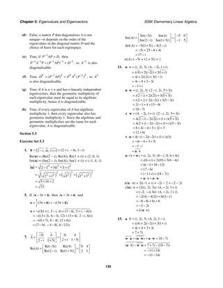
![Chapter 5: Eigenvalues and Eigenvectors SSM: Elementary Linear Algebra
132
Thus, 1
A PCP−
= where
1 1
1 0
P
−
⎡ ⎤
= ⎢ ⎥
−
⎣ ⎦
and
5 3
3 5
.
C
−
⎡ ⎤
= ⎢ ⎥
⎣ ⎦
27. (a) 3 6
2 6 3
2 6 3
8 3
, , ) ( , , )
( ) ( ) ( )
i i i i i k
i i i i i k
ik
ik
⋅ = (2 ⋅
= − + − +
= + +
= +
u v
If u ⋅ v = 0, then 3 8
ik = − or
8 8
3 3
k i
i
= − =
so
8
3
.
k i
=
(b)
2
1 1 1 1
1 1 1 1
1
2
( , , ) ( , , )
( ) ( ) ( )( )
( )
k k i i
k k i i
i
i
⋅ = + ⋅ − −
= + − + + +
= +
=
u v
Thus, there is no complex scalar k for which
u ⋅ v = 0.
True/False 5.3
(a) False; non-real complex eigenvalues occur in
conjugate pairs, so there must be an even
number. Since a real 5 × 5 matrix will have 5
eigenvalues, at least one must be real.
(b) True; 2
Tr 0
( ) det( )
A A
λ − λ + = is the
characteristic equation of a 2 × 2 matrix A.
(c) False; if A is a matrix with real entries and
complex eigenvalues and k is a real scalar,
k ≠ 0, 1, then kA has the same eigenvalues as A
with the same algebraic multiplicities but
tr(kA) = ktr(A) ≠ tr(A).
(d) True; complex eigenvalues and eigenvectors
occur in conjugate pairs.
(e) False; real symmetric matrices have real
eigenvalues.
(f) False; this is only true if the eigenvalues of A
satisfy 1.
=
λ
Section 5.4
Exercise Set 5.4
1. (a) The coefficient matrix for the system is
1 4
2 3
.
A
⎡ ⎤
= ⎢ ⎥
⎣ ⎦
2
det 4 5 5 1
( ) ( )( )
I A
λ − = λ − λ − = λ − λ +
The eigenvalues of A are 1 5
λ = and
2 1.
λ = −
(λI − A)x = 0 is 1
2
1 4 0
2 3 0
.
x
x
λ − − ⎡ ⎤
⎡ ⎤ ⎡ ⎤
=
⎢ ⎥
⎢ ⎥ ⎢ ⎥
− λ −
⎣ ⎦ ⎣ ⎦
⎣ ⎦
1 5
λ = gives 1
2
4 4 0
2 2 0
.
x
x
− ⎡ ⎤
⎡ ⎤ ⎡ ⎤
=
⎢ ⎥
⎢ ⎥ ⎢ ⎥
−
⎣ ⎦ ⎣ ⎦
⎣ ⎦
Since
4 4
2 2
−
⎡ ⎤
⎢ ⎥
−
⎣ ⎦
reduces to
1 1
0 0
−
⎡ ⎤
⎢ ⎥
⎣ ⎦
a
general solution is 1 ,
x s
= 2 ,
x s
= or
1
2
1
1
x
s
x
⎡ ⎤ ⎡ ⎤
=
⎢ ⎥ ⎢ ⎥
⎣ ⎦
⎣ ⎦
and 1
1
1
⎡ ⎤
= ⎢ ⎥
⎣ ⎦
p is a basis for the
eigenspace corresponding to 1 5.
λ =
2 1
λ = − gives 1
2
2 4 0
2 4 0
.
x
x
− − ⎡ ⎤
⎡ ⎤ ⎡ ⎤
=
⎢ ⎥
⎢ ⎥ ⎢ ⎥
− −
⎣ ⎦ ⎣ ⎦
⎣ ⎦
Since
2 4
2 4
− −
⎡ ⎤
⎢ ⎥
− −
⎣ ⎦
reduces to
1 2
0 0
⎡ ⎤
⎢ ⎥
⎣ ⎦
a
general solution is 1 2 ,
x s
= − 2
x s
= or
1
2
2
1
x
x
−
⎡ ⎤ ⎡ ⎤
=
⎢ ⎥ ⎢ ⎥
⎣ ⎦
⎣ ⎦
and 2
2
1
−
⎡ ⎤
= ⎢ ⎥
⎣ ⎦
p is a basis for
the eigenspace corresponding to 2 1.
λ = −
Thus 1 2
1 2
1 1
[ ]
P
−
⎡ ⎤
= = ⎢ ⎥
⎣ ⎦
p p diagonalizes
A and 1 1
2
0 5 0
0 0 1
.
P AP D
− λ
⎡ ⎤ ⎡ ⎤
= = =
⎢ ⎥ ⎢ ⎥
λ −
⎣ ⎦
⎣ ⎦
The substitutions y = Pu and P
′ ′
=
y u give
the “diagonal system”
5 0
0 1
D
⎡ ⎤
′ = = ⎢ ⎥
−
⎣ ⎦
u u u
or 1 1
2 2
5
u u
u u
′ =
′ = −
which has the solution
5
1
2
.
x
x
c e
c e−
⎡ ⎤
= ⎢ ⎥
⎢ ⎥
⎣ ⎦
u Then y = Pu gives the
solution
5 5
1 1 2
5
2 1 2
2
1 2
1 1
x x x
x x x
c e c e c e
c e c e c e
−
− −
⎡ ⎤ ⎡ ⎤
−
−
⎡ ⎤
= =
⎢ ⎥ ⎢ ⎥
⎢ ⎥
⎣ ⎦ +
⎢ ⎥ ⎢ ⎥
⎣ ⎦ ⎣ ⎦
y and](https://image.slidesharecdn.com/elementary-linear-algebra-chapter1-220420115526/85/Elementary-linear-algebra-chapter-1-pdf-187-320.jpg)
![SSM: Elementary Linear Algebra Section 5.4
133
the solution of the system is
5
1 1 2
5
2 1 2
2
x x
x x
y c e c e
y c e c e
−
−
= −
= +
.
(b) The initial conditions give 1 2
1 2
2 0
0
c c
c c
− =
+ =
which has the solution 1 2 0,
c c
= = so the
solution satisfying the given initial
conditions is 1
2
0
0
y
y
=
=
.
3. (a) The coefficient matrix for the system is
4 0 1
2 1 0
2 0 1
.
A
⎡ ⎤
⎢ ⎥
= −
⎢ ⎥
−
⎣ ⎦
3 2
6 11 6
1 2 3
det( )
( )( )( )
I A
λ − = λ − λ + λ −
= λ − λ − λ −
The eigenvalues of A are 1 1,
λ = 2 2,
λ =
and 3 3.
λ =
(λI − A)x = 0 is
1
2
3
4 0 1 0
2 1 0 0
2 0 1 0
.
x
x
x
⎡ ⎤
λ − −
⎡ ⎤ ⎡ ⎤
⎢ ⎥
⎢ ⎥ ⎢ ⎥
=
λ −
⎢ ⎥
⎢ ⎥ ⎢ ⎥
λ −
⎣ ⎦ ⎣ ⎦
⎣ ⎦
1 1
λ = gives
1
2
3
3 0 1 0
2 0 0 0
2 0 0 0
.
x
x
x
⎡ ⎤
− −
⎡ ⎤ ⎡ ⎤
⎢ ⎥
⎢ ⎥ ⎢ ⎥
=
⎢ ⎥
⎢ ⎥ ⎢ ⎥
⎣ ⎦ ⎣ ⎦
⎣ ⎦
Since
3 0 1
2 0 0
2 0 0
− −
⎡ ⎤
⎢ ⎥
⎢ ⎥
⎣ ⎦
reduces to
1 0 0
0 0 1
0 0 0
,
⎡ ⎤
⎢ ⎥
⎢ ⎥
⎣ ⎦
the general solution is 1 0,
x = 2 ,
x s
=
3 0
x = or
1
2
3
0
1
0
x
x s
x
⎡ ⎤ ⎡ ⎤
⎢ ⎥ ⎢ ⎥
=
⎢ ⎥ ⎢ ⎥
⎣ ⎦
⎣ ⎦
and 1
0
1
0
⎡ ⎤
⎢ ⎥
=
⎢ ⎥
⎣ ⎦
p is a
basis for the eigenspace corresponding to
1 1.
λ =
2 2
λ = gives
1
1
3
2 0 1 0
2 1 0 0
2 0 1 0
.
x
x
x
⎡ ⎤
− −
⎡ ⎤ ⎡ ⎤
⎢ ⎥
⎢ ⎥ ⎢ ⎥
=
⎢ ⎥
⎢ ⎥ ⎢ ⎥
⎣ ⎦ ⎣ ⎦
⎣ ⎦
Since
2 0 1
2 1 0
2 0 1
− −
⎡ ⎤
⎢ ⎥
⎢ ⎥
⎣ ⎦
reduces to
1
2
1 0
0 1 1
0 0 0
,
⎡ ⎤
⎢ ⎥
−
⎢ ⎥
⎢ ⎥
⎣ ⎦
the general solution is
1
1
2
,
x s
= − 2 ,
x s
= 3
x s
= or 1 ,
x t
= −
2 2 ,
x t
= 3 2
x t
= which is
1
2
3
1
2
2
x
x t
x
⎡ ⎤ −
⎡ ⎤
⎢ ⎥ ⎢ ⎥
=
⎢ ⎥ ⎢ ⎥
⎣ ⎦
⎣ ⎦
and 2
1
2
2
−
⎡ ⎤
⎢ ⎥
=
⎢ ⎥
⎣ ⎦
p is a basis for the eigenspace
corresponding to 2 2.
λ =
3 3
λ = gives
1
2
3
1 0 1 0
2 2 0 0
2 0 2 0
.
x
x
x
⎡ ⎤
− −
⎡ ⎤ ⎡ ⎤
⎢ ⎥
⎢ ⎥ ⎢ ⎥
=
⎢ ⎥
⎢ ⎥ ⎢ ⎥
⎣ ⎦ ⎣ ⎦
⎣ ⎦
Since
1 0 1
2 2 0
2 0 2
− −
⎡ ⎤
⎢ ⎥
⎢ ⎥
⎣ ⎦
reduces to
1 0 1
0 1 1
0 0 0
,
⎡ ⎤
⎢ ⎥
−
⎢ ⎥
⎣ ⎦
the general solution is 1 ,
x s
=
2 ,
x s
= − 3
x s
= − or
1
2
3
1
1
1
x
x s
x
⎡ ⎤ ⎡ ⎤
⎢ ⎥ ⎢ ⎥
= −
⎢ ⎥ ⎢ ⎥
−
⎣ ⎦
⎣ ⎦
and
3
1
1
1
⎡ ⎤
⎢ ⎥
= −
⎢ ⎥
−
⎣ ⎦
p is a basis for the eigenspace
corresponding to 3 3.
λ =
Thus 1 2 3
0 1 1
1 2 1
0 2 1
[ ]
P
−
⎡ ⎤
⎢ ⎥
= = −
⎢ ⎥
−
⎣ ⎦
p p p
diagonalizes A and
1
1
2
3
0 0 1 0 0
0 0 0 2 0
0 0 3
0 0
.
P AP D
−
λ
⎡ ⎤ ⎡ ⎤
⎢ ⎥ ⎢ ⎥
λ
= = =
⎢ ⎥ ⎢ ⎥
λ ⎣ ⎦
⎣ ⎦
The substitutions y = Pu and P
′ ′
=
y u give
the “diagonal system”
1 0 0
0 2 0
0 0 3
D
⎡ ⎤
⎢ ⎥
′ = =
⎢ ⎥
⎣ ⎦
u u u or
1 1
2 2
3 3
2
3
u u
u u
u u
′ =
′ =
′ =
which
has the solution
1
2
2
3
3
.
x
x
x
c e
c e
c e
⎡ ⎤
⎢ ⎥
= ⎢ ⎥
⎢ ⎥
⎣ ⎦
u Then y = Pu
gives the solution](https://image.slidesharecdn.com/elementary-linear-algebra-chapter1-220420115526/85/Elementary-linear-algebra-chapter-1-pdf-188-320.jpg)
![Chapter 5: Eigenvalues and Eigenvectors SSM: Elementary Linear Algebra
134
1
2
2
3
3
2 3
2 3
2 3
1 2 3
2 3
2 3
0 1 1
1 2 1
0 2 1
2
2
x
x
x
x x
x x x
x x
c e
c e
c e
c e c e
c e c e c e
c e c e
⎡ ⎤
−
⎡ ⎤ ⎢ ⎥
⎢ ⎥
= − ⎢ ⎥
⎢ ⎥ ⎢ ⎥
−
⎣ ⎦
⎣ ⎦
⎡ ⎤
− +
⎢ ⎥
= + −
⎢ ⎥
⎢ ⎥
−
⎣ ⎦
y
and the solution of the system is
2 3
1 2 3
2 3
2 1 2 3
2 3
3 2 3
2
2
.
x x
x x x
x x
y c e c e
y c e c e c e
y c e c e
= − +
= + −
= −
(b) The initial conditions give
2 3
1 2 3
2 3
1
2 1
2 0
c c
c c c
c c
− + = −
+ − =
− =
which has the solution 1 1,
c = 2 1,
c = −
3 2,
c = − so the solution satisfying the given
initial conditions is
2 3
1
2 3
2
2 3
3
2
2 2
2 2
.
x x
x x x
x x
y e e
y e e e
y e e
= −
= − +
= − +
5. Let y = f(x) be a solution of .
y ay
′ = Then for
( ) ( ) ax
g x f x e−
= we have
0
( ) ( ) ( )( )
( ) ( )
ax ax
ax ax
g x f x e f x ae
af x e af x e
− −
− −
′ ′
= + −
= −
=
Hence ( ) ( ) ax
g x f x e c
−
= = where c is a
constant or ( ) .
ax
f x ce
=
7. If 1
y y
= and 2 ,
y y′
= then
2 2 1
6 6
y y y y y y
′ ′′ ′
= = + = + which yields the
system
1 2
2 1 2
6
y y
y y y
′ =
′ = +
The coefficient matrix of this system is
0 1
6 1
.
A
⎡ ⎤
= ⎢ ⎥
⎣ ⎦
2
6 3 2
det( ) ( )( )
I A
λ − = λ − λ − = λ − λ +
The eigenvalues of A are 1 3
λ = and 2 2.
λ = −
( )
I A
λ − =
x 0 is 1
2
1 0
6 1 0
.
x
x
λ − ⎡ ⎤
⎡ ⎤ ⎡ ⎤
=
⎢ ⎥
⎢ ⎥ ⎢ ⎥
− λ −
⎣ ⎦ ⎣ ⎦
⎣ ⎦
1 3
λ = gives 1
2
3 1 0
6 2 0
.
x
x
− ⎡ ⎤
⎡ ⎤ ⎡ ⎤
=
⎢ ⎥
⎢ ⎥ ⎢ ⎥
−
⎣ ⎦ ⎣ ⎦
⎣ ⎦
Since
3 1
6 2
−
⎡ ⎤
⎢ ⎥
−
⎣ ⎦
reduces to
1
3
1
0 0
,
⎡ ⎤
−
⎢ ⎥
⎣ ⎦
the
general solution is 1
1
3
,
x s
= 2
x s
= or 1 ,
x t
=
2 3
x t
= which is 1
2
1
3
,
x
t
x
⎡ ⎤ ⎡ ⎤
=
⎢ ⎥ ⎢ ⎥
⎣ ⎦
⎣ ⎦
so 1
1
3
⎡ ⎤
= ⎢ ⎥
⎣ ⎦
p is a
basis for the eigenspace corresponding to
1 3.
λ =
2 2
λ = − gives 1
2
2 1 0
6 3 0
.
x
x
− − ⎡ ⎤
⎡ ⎤ ⎡ ⎤
=
⎢ ⎥
⎢ ⎥ ⎢ ⎥
− −
⎣ ⎦ ⎣ ⎦
⎣ ⎦
Since
2 1
6 3
− −
⎡ ⎤
⎢ ⎥
− −
⎣ ⎦
reduces to
1
2
1
0 0
,
⎡ ⎤
⎢ ⎥
⎣ ⎦
the general
solution is 1
1
2
,
x s
= − 2
x s
= or 1 ,
x t
=
2 2
x t
= − which is 1
2
1
2
x
t
x
⎡ ⎤ ⎡ ⎤
=
⎢ ⎥ ⎢ ⎥
−
⎣ ⎦
⎣ ⎦
so 2
1
2
⎡ ⎤
= ⎢ ⎥
−
⎣ ⎦
p
is a basis for the eigenspace corresponding to
2 2.
λ = − Thus [ ]
1 2
1 1
3 2
P
⎡ ⎤
= = ⎢ ⎥
−
⎣ ⎦
p p
diagonalizes A and
1 1
2
0 3 0
0 0 2
.
P AP D
− λ
⎡ ⎤ ⎡ ⎤
= = =
⎢ ⎥ ⎢ ⎥
λ −
⎣ ⎦
⎣ ⎦
The substitutions y = Pu and P
′ ′
=
y u give the
“diagonal system”
3 0
0 2
D
⎡ ⎤
′ = = ⎢ ⎥
−
⎣ ⎦
u u u or
1 1
2 2
3
2
u u
u u
′ =
′ = −
which has the solution
3
1
2
2
.
x
x
c e
c e−
⎡ ⎤
= ⎢ ⎥
⎢ ⎥
⎣ ⎦
u Then
y = Pu gives the solution
3 3 2
1 1 2
2 3 2
2 1 2
1 1
3 2 3 2
.
x x x
x x x
c e c e c e
c e c e c e
−
− −
⎡ ⎤ ⎡ ⎤
+
⎡ ⎤
= =
⎢ ⎥ ⎢ ⎥
⎢ ⎥
−
⎣ ⎦ −
⎢ ⎥ ⎢ ⎥
⎣ ⎦ ⎣ ⎦
y
Thus 3 2
1 1 2
x x
y y c e c e−
= = + is the solution of
the original differential equation.
9. Use the substitutions 1 ,
y y
= 2 1
y y y
′ ′
= = and
3 2.
y y y
′′ ′
= = This gives the system
0 1 0
0 0 1
6 11 6
.
A
⎡ ⎤
⎢ ⎥
=
⎢ ⎥
−
⎣ ⎦](https://image.slidesharecdn.com/elementary-linear-algebra-chapter1-220420115526/85/Elementary-linear-algebra-chapter-1-pdf-189-320.jpg)
![SSM: Elementary Linear Algebra Section 5.4
135
3 2
6 11 6
1 2 3
det( )
( )( )( )
I A
λ − = λ − λ + λ −
= λ − λ − λ −
The eigenvalues of A are 1 1,
λ = 2 2,
λ = and
3 3.
λ =
( )
I A
λ − =
x 0 is
1
2
3
1 0 0
0 1 0
6 11 6 0
.
x
x
x
⎡ ⎤
λ −
⎡ ⎤ ⎡ ⎤
⎢ ⎥
⎢ ⎥ ⎢ ⎥
=
λ −
⎢ ⎥
⎢ ⎥ ⎢ ⎥
− λ −
⎣ ⎦ ⎣ ⎦
⎣ ⎦
1 1
λ = gives
1
2
3
1 1 0 0
0 1 1 0
6 11 5 0
.
x
x
x
⎡ ⎤
−
⎡ ⎤ ⎡ ⎤
⎢ ⎥
⎢ ⎥ ⎢ ⎥
=
−
⎢ ⎥
⎢ ⎥ ⎢ ⎥
− −
⎣ ⎦ ⎣ ⎦
⎣ ⎦
Since
1 1 0
0 1 1
6 11 5
−
⎡ ⎤
⎢ ⎥
−
⎢ ⎥
− −
⎣ ⎦
reduces to
1 0 1
0 1 1
0 0 0
,
−
⎡ ⎤
⎢ ⎥
−
⎢ ⎥
⎣ ⎦
the general solution is 1 ,
x s
= 2 ,
x s
= 3
x s
= or
1
2
3
1
1
1
x
x s
x
⎡ ⎤ ⎡ ⎤
⎢ ⎥ ⎢ ⎥
=
⎢ ⎥ ⎢ ⎥
⎣ ⎦
⎣ ⎦
so 1
1
1
1
⎡ ⎤
⎢ ⎥
=
⎢ ⎥
⎣ ⎦
p is a basis for the
eigenspace corresponding to 1 1.
λ =
2 2
λ = gives
1
2
3
2 1 0 0
0 2 1 0
6 11 4 0
.
x
x
x
⎡ ⎤
−
⎡ ⎤ ⎡ ⎤
⎢ ⎥
⎢ ⎥ ⎢ ⎥
=
−
⎢ ⎥
⎢ ⎥ ⎢ ⎥
− −
⎣ ⎦ ⎣ ⎦
⎣ ⎦
Since
2 1 0
0 2 1
−
⎡ ⎤
⎢ ⎥
−
⎣ ⎦
reduces to
1
4
1
2
1 0
0 1
0 0 0
,
⎡ ⎤
−
⎢ ⎥
−
⎢ ⎥
⎢ ⎥
⎣ ⎦
the general solution is 1
1
4
,
x s
= 2
1
2
,
x s
=
3
x s
= or 1 ,
x t
= 2 2 ,
x t
= 3 4
x t
= which is
1
2
3
1
2
4
x
x t
x
⎡ ⎤ ⎡ ⎤
⎢ ⎥ ⎢ ⎥
=
⎢ ⎥ ⎢ ⎥
⎣ ⎦
⎣ ⎦
so 2
1
2
4
⎡ ⎤
⎢ ⎥
=
⎢ ⎥
⎣ ⎦
p is a basis for the
eigenspace corresponding to 2 2.
λ =
3 3
λ = gives
1
2
3
3 1 0 0
0 3 1 0
6 11 3 0
.
x
x
x
⎡ ⎤
−
⎡ ⎤ ⎡ ⎤
⎢ ⎥
⎢ ⎥ ⎢ ⎥
=
−
⎢ ⎥
⎢ ⎥ ⎢ ⎥
− −
⎣ ⎦ ⎣ ⎦
⎣ ⎦
Since
3 1 0
0 3 1
6 11 3
−
⎡ ⎤
⎢ ⎥
−
⎢ ⎥
− −
⎣ ⎦
reduces to
1
9
1
3
1 0
0 1
0 0 0
,
⎡ ⎤
−
⎢ ⎥
−
⎢ ⎥
⎢ ⎥
⎣ ⎦
the general solution is 1
1
9
,
x s
= 2
1
3
,
x s
=
3
x s
= or 1 ,
x t
= 2 3 ,
x t
= 3 9
x t
= which is
1
2
3
1
3
9
x
x t
x
⎡ ⎤ ⎡ ⎤
⎢ ⎥ ⎢ ⎥
=
⎢ ⎥ ⎢ ⎥
⎣ ⎦
⎣ ⎦
so 3
1
3
9
⎡ ⎤
⎢ ⎥
=
⎢ ⎥
⎣ ⎦
p is a basis for the
eigenspace corresponding to 3 3.
λ =
Thus 1 2 3
1 1 1
1 2 3
1 4 9
[ ]
P
⎡ ⎤
⎢ ⎥
= =
⎢ ⎥
⎣ ⎦
p p p
diagonalizes A and
1
1
2
3
0 0 1 0 0
0 0 0 2 0
0 0 3
0 0
.
P AP D
−
λ
⎡ ⎤ ⎡ ⎤
⎢ ⎥ ⎢ ⎥
λ
= = =
⎢ ⎥ ⎢ ⎥
λ ⎣ ⎦
⎣ ⎦
The substitutions y = Pu and P
′ ′
=
y u give the
“diagonal system”
1 0 0
0 2 0
0 0 3
D
⎡ ⎤
⎢ ⎥
′ = =
⎢ ⎥
⎣ ⎦
u u u or
1 1
2 2
3 3
2
3
u u
u u
u u
′ =
′ =
′ =
which has the solution
1
2
2
3
3
.
x
x
x
c e
c e
c e
⎡ ⎤
⎢ ⎥
= ⎢ ⎥
⎢ ⎥
⎣ ⎦
u
Then y = Pu gives the solution
1
2
2
3
3
2 3
1 2 3
2 3
1 2 3
2 3
1 2 3
1 1 1
1 2 3
1 4 9
2 3
4 9
.
x
x
x
x x x
x x x
x x x
c e
c e
c e
c e c e c e
c e c e c e
c e c e c e
⎡ ⎤
⎡ ⎤ ⎢ ⎥
⎢ ⎥
= ⎢ ⎥
⎢ ⎥ ⎢ ⎥
⎣ ⎦
⎣ ⎦
⎡ ⎤
+ +
⎢ ⎥
= + +
⎢ ⎥
⎢ ⎥
+ +
⎣ ⎦
y
Thus 2 3
1 1 2 3
x x x
y y c e c e c e
= = + + is the
solution of the original differential equation.
True/False 5.4
(a) False; just as not every system Ax = b has a
solution, not every system of differential
equations has a solution.
(b) False; x and y may differ by any constant vector
b.
(c) True
(d) True; if A is a square matrix with distinct real
eigenvalues, it is diagonalizable.
(e) False; consider the case where A is
diagonalizable but not diagonal. Then A is
similar to a diagonal matrix P which can be used
to solve the system ,
A
′ =
y y but the systems
A
′ =
y y and P
′ =
u u do not have the same
solutions.](https://image.slidesharecdn.com/elementary-linear-algebra-chapter1-220420115526/85/Elementary-linear-algebra-chapter-1-pdf-190-320.jpg)
![138
Chapter 6
Inner Product Spaces
Section 6.1
Exercise Set 6.1
1. (a) 1 3 1 2 5
, = ⋅ + ⋅ =
u v
(b) 9 0 6 1 6
3 ( )
, ,
k = = ⋅ + ⋅ − = −
v w v w
(c)
1 0 1 1 3 0 2 1
3
, , ,
( ) ( )
= +
+
= ⋅ + ⋅ − + ⋅ + ⋅ −
= −
u v w u w v w
(d) 2 2
3 2 13
,
= = + =
v v
v
(e)
2 2
2 1
2 1
5
( , )
( , )
( ) ( )
d = −
= − −
= − + −
=
u v u v
(f)
2 2
1 1 3 3 2
8 5
8 5
89
( , ) ( , )
( , )
( ) ( )
k = −
−
= − −
= − + −
=
u v
3. (a) 3 4 2 5 2
( ) ( )( )
, = + − =
u v
4 3 5 2 2
( ) ( )
, = + − =
v u
(b) 7 3 1 6
7 1 3 6
11
, ( , ), ( , )
( ) ( )
=
+ −
= − +
=
u v w
3 1 2 6 4 1 5 6
15 26
11
, ,
( ( ) ( )( )) ( ( ) ( ))
+
= − + − + − +
= − +
=
u w v w
(c) 3 2 3 11
3 3 2 11
13
, ( , ), ( , )
( ) ( )( )
=
+ −
= + −
= −
u v w
3 4 2 5 3 1 2 6
2 15
13
, ,
( ( ) ( )( )) ( ( ) ( )( ))
+
= + − + − + −
= −
= −
u v u w
(d) 12 8 4 5
12 4 8 5
8
, ( , ), ( , )
( ) ( )
k = −
= − +
= −
u v
4 2 8
( )
,
k = − = −
u v
3 2 16 20
3 16 2 20
8
, ( , ), ( , )
( ) ( )( )
k = − − −
= − + − −
= −
u v
(e) 0 4 0 5 0
0 0 4 5 ( ) ( )
, ( , ), ( , )
= = + =
0 v
4 0 5 0 0
4 5 0 0 ( ) ( )
, ( , ), ( , )
= = + =
v 0
5. Let
2 1
1 1
.
A
⎡ ⎤
= ⎢ ⎥
⎣ ⎦
Then
2 1
1 1
T
A A
⎡ ⎤
= =
⎢ ⎥
⎣ ⎦
so
2 5 3
3 2
.
T
A A A
⎡ ⎤
= = ⎢ ⎥
⎣ ⎦
(a)
5 3 2
1 1
3 2 1
2
2 1
1
4 1
5
,
[ ]
[ ]
T T
A A
=
⎡ ⎤ ⎡ ⎤
= − ⎢ ⎥ ⎢ ⎥
⎣ ⎦ ⎣ ⎦
⎡ ⎤
= − − ⎢ ⎥
⎣ ⎦
= − −
= −
v u
u v
(b)
5 3 1
0 1
3 2 1
1
3 2
1
3 2
1
,
[ ]
[ ]
T T
A A
=
−
⎡ ⎤ ⎡ ⎤
= − ⎢ ⎥ ⎢ ⎥
⎣ ⎦ ⎣ ⎦
−
⎡ ⎤
= − − ⎢ ⎥
⎣ ⎦
= −
=
w v
v w
(c)
5 3 1
0 1
3 2 2
1
3 2
2
3 4
7
( )
,
[ ]
[ ]
T T
A A
= +
+
⎡ ⎤ ⎡ ⎤
= − ⎢ ⎥ ⎢ ⎥
⎣ ⎦ ⎣ ⎦
⎡ ⎤
= − − ⎢ ⎥
⎣ ⎦
= − −
= −
w u v
u v w](https://image.slidesharecdn.com/elementary-linear-algebra-chapter1-220420115526/85/Elementary-linear-algebra-chapter-1-pdf-193-320.jpg)
![SSM: Elementary Linear Algebra Section 6.1
139
(d)
5 3 1
1 1
3 2 1
1
2 1
1
2 1
1
,
[ ]
[ ]
T T
A A
=
−
⎡ ⎤ ⎡ ⎤
= − ⎢ ⎥ ⎢ ⎥
⎣ ⎦ ⎣ ⎦
−
⎡ ⎤
= − − ⎢ ⎥
⎣ ⎦
= −
=
v v
v v
1 1
,
= = =
v v
v
(e)
1 0 1
1 1 2
− −
⎡ ⎤ ⎡ ⎤ ⎡ ⎤
− = − =
⎢ ⎥ ⎢ ⎥ ⎢ ⎥
−
⎣ ⎦ ⎣ ⎦ ⎣ ⎦
v w
5 3 1
1 2
3 2 2
1
1 1
2
1 2
1
( ) ( )
,
[ ]
[ ]
T T
A A
= − −
− −
−
⎡ ⎤ ⎡ ⎤
= − ⎢ ⎥ ⎢ ⎥
⎣ ⎦ ⎣ ⎦
−
⎡ ⎤
= ⎢ ⎥
⎣ ⎦
= − +
=
v w v w
v w v w
1
1
( , )
,
d = −
= − −
=
=
v w v w
v w v w
(f) 2 2
2
1 1
( ( , ))
d
= = =
− v w
v w
7. (a)
3 4 1 3 1 13
2 8 1 1 10 2
T −
⎡ ⎤ ⎡ ⎤ ⎡ ⎤
= =
⎢ ⎥ ⎢ ⎥ ⎢ ⎥
−
⎣ ⎦ ⎣ ⎦ ⎣ ⎦
u v
tr 1 2 3
( )
, T
= = + =
u v
u v
(b)
1 3 4 6 4 18
2 5 0 8 8 52
T − −
⎡ ⎤ ⎡ ⎤ ⎡ ⎤
= =
⎢ ⎥ ⎢ ⎥ ⎢ ⎥
⎣ ⎦ ⎣ ⎦ ⎣ ⎦
u v
tr 4 52 56
( )
, T
= = + =
u v
u v
9. (a)
3 0
0 2
,
T
A A
⎡ ⎤
= =
⎢ ⎥
⎣ ⎦
so 2 9 0
0 4
.
T
A A A
⎡ ⎤
= = ⎢ ⎥
⎣ ⎦
For 1
2
u
u
⎡ ⎤
= ⎢ ⎥
⎣ ⎦
u and 1
2
,
v
v
⎡ ⎤
= ⎢ ⎥
⎣ ⎦
v
1
1 2
2
1
1 2
2
1 1 2 2
9 0
0 4
9 4
9 4
,
[ ]
[ ]
T T
A A
u
v v
u
u
v v
u
u v u v
=
⎡ ⎤
⎡ ⎤
= ⎢ ⎥
⎢ ⎥
⎣ ⎦ ⎣ ⎦
⎡ ⎤
= ⎢ ⎥
⎣ ⎦
= +
v u
u v
(b) 9 3 1 4 2 7 27 56 29
( )( ) ( )( )
, = − + = − + =
u v
11. (a) The matrix is
3 0
0 5
,
A
⎡ ⎤
= ⎢ ⎥
⎣ ⎦
since
2 3 0
0 5
.
T
A A A
⎡ ⎤
= = ⎢ ⎥
⎣ ⎦
(b) The matrix is
2 0
0 6
,
A
⎡ ⎤
= ⎢ ⎥
⎣ ⎦
since
2 4 0
0 6
.
T
A A A
⎡ ⎤
= = ⎢ ⎥
⎣ ⎦
13. (a)
2 2 2 2
2 5 3 6
74
,
( )
A A
A =
= − + + +
=
(b) 0
A = by inspection.
15. (a)
6 1
8 2
A B
−
⎡ ⎤
− = ⎢ ⎥
−
⎣ ⎦
2 2 2 2
6 1 8 2
105
( , )
,
( ) ( )
d A B A B
A B A B
= −
= − −
= + − + + −
=
(b)
3 3
5 2
A B
⎡ ⎤
− = ⎢ ⎥
− −
⎣ ⎦
2 2 2 2
3 3 5 2
47
( , )
,
( ) ( )
d A B A B
A B A B
= −
= − −
= + + − + −
=
17.
1 1 0 0 1 1 2 2
2 2 0 1 2 2 10 5
4 0 4 50
50
,
( ) ( ) ( ) ( ) ( ) ( ) ( ) ( )
( )( ) ( )( ) ( )( ) ( )( )
p q p q p q p q
= − − + + +
= − + + +
= − + + +
=
p q
2 2 2 2
2 2 2 2
1 0 1 2
2 0 2 10
108
6 3
,
[ ( )] [ ( )] [ ( )] [ ( )]
( )
p p p p
=
= − + + +
= − + + +
=
=
p p p](https://image.slidesharecdn.com/elementary-linear-algebra-chapter1-220420115526/85/Elementary-linear-algebra-chapter-1-pdf-194-320.jpg)
![Chapter 6: Inner Product Spaces SSM: Elementary Linear Algebra
140
19. u − v = (−3, −3)
(a)
2 2
3 3
18
3 2
( , )
,
( ) ( )
d = −
= − −
= − + −
=
=
u v u v
u v u v
(b)
2 2
3 3 2 3
45
3 5
( , )
,
( ) ( )
d = −
= − −
= − + −
=
=
u v u v
u v u v
(c)
1 1 1 2 2 1
2 3 1 3 1 13
T
A A
− −
⎡ ⎤ ⎡ ⎤ ⎡ ⎤
= =
⎢ ⎥ ⎢ ⎥ ⎢ ⎥
− −
⎣ ⎦ ⎣ ⎦ ⎣ ⎦
2 1 3
3 3
1 13 3
3
3 36
3
9 108
117
( ) ( )
,
[ ]
[ ]
T T
A A
= − −
− −
− −
⎡ ⎤ ⎡ ⎤
= − − ⎢ ⎥ ⎢ ⎥
− −
⎣ ⎦ ⎣ ⎦
−
⎡ ⎤
= − − ⎢ ⎥
−
⎣ ⎦
= +
=
u v u v
u v u v
117
3 13
( , )
,
d = −
= − −
=
=
u v u v
u v u v
21. (a) For u = (x, y),
1 2 2 2
1 1
4 16
/
, x y
= = +
u u
u and the unit circle is 2 2
1 1
1
4 16
x y
+ = or
2 2
1
4 16
x y
+ = which
is the ellipse shown.
y
x
2
–2
4
–4](https://image.slidesharecdn.com/elementary-linear-algebra-chapter1-220420115526/85/Elementary-linear-algebra-chapter-1-pdf-195-320.jpg)
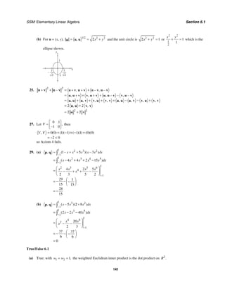
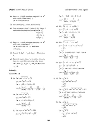
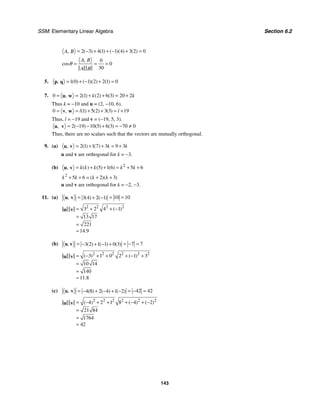
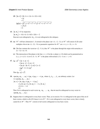
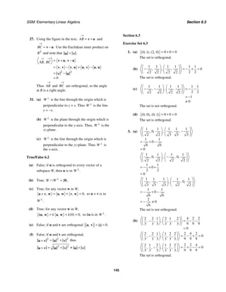
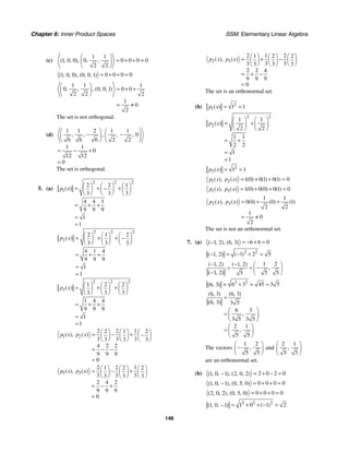
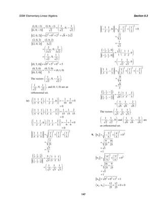
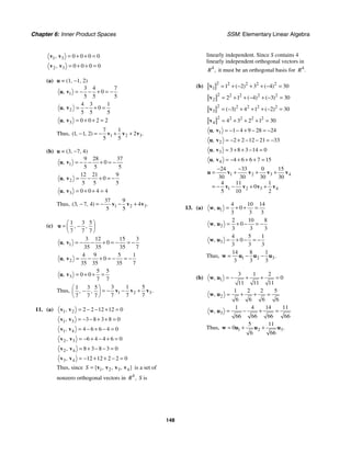
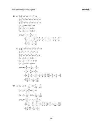
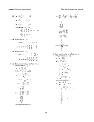
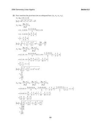
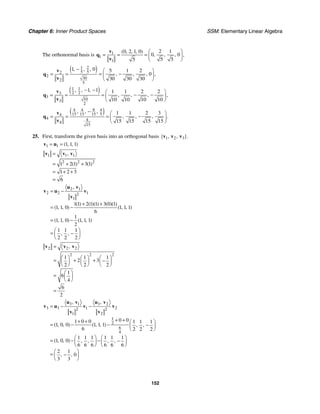
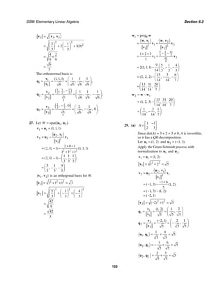
![Chapter 6: Inner Product Spaces SSM: Elementary Linear Algebra
154
The QR-decomposition of A is
1 1 2 1
1 2
2 2
1 2
5 5
2 1
5 5
1 1
2 3 0
5 5
0 5
, ,
[ ]
,
.
⎡ ⎤
−
⎡ ⎤
= ⎢ ⎥
⎢ ⎥
⎣ ⎦ ⎣ ⎦
⎡ ⎤
− ⎡ ⎤
⎢ ⎥
= ⎢ ⎥
⎢ ⎥ ⎣ ⎦
⎣ ⎦
u q u q
q q
u q
(b)
1 2
0 1
1 4
A
⎡ ⎤
⎢ ⎥
=
⎢ ⎥
⎣ ⎦
By inspection, the column vectors of A are
linearly independent, so A has a
QR-decomposition. Let 1 1 0 1
( , , )
=
u and
2 2 1 4
( , , ).
=
u
Apply the Gram-Schmidt process with
normalization to 1
u and 2.
u
1 1 1 0 1
( , , )
= =
v u
2 2 2
1 1 0 1 2
= + + =
v
2 1
2 2 1
2
1
2 0 4
2 1 4 1 0 1
2
2 1 4 3 0 3
1 1 1
,
( , , ) ( , , )
( , , ) ( , , )
( , , )
= −
+ +
= −
= −
= −
u v
v u v
v
2 2 2
2 1 1 1 3
( )
= − + + =
v
1
1
1
1 1
1 0 1
0
2 2
2
( , , )
, ,
⎛ ⎞
= = = ⎜ ⎟
⎝ ⎠
v
q
v
2
2
2
1 1 1
1 1 1
3 3 3
3
( , , )
, ,
− ⎛ ⎞
−
= = = ⎜ ⎟
⎝ ⎠
v
q
v
1 1
1 1
0 2
2 2
, = + + =
u q
2 1
2 4
0 3 2
2 2
, = + + =
u q
2 2
2 1 4
3
3 3 3
, = − + + =
u q
The QR-decomposition of A is
1 1 2 1
1 2
2 2
1 1
2 3
1
3
1 1
2 3
1 2
0 1
0
1 4
2 3 2
0
0 3
, ,
[ ]
,
⎡ ⎤ ⎡ ⎤
⎢ ⎥ = ⎢ ⎥
⎢ ⎥ ⎣ ⎦
⎣ ⎦
⎡ ⎤
−
⎢ ⎥
⎡ ⎤
⎢ ⎥
= ⎢ ⎥
⎢ ⎥ ⎣ ⎦
⎢ ⎥
⎢ ⎥
⎣ ⎦
u q u q
q q
u q
(c)
1 1
2 1
2 1
A
⎡ ⎤
⎢ ⎥
= −
⎢ ⎥
⎣ ⎦
By inspection, the column vectors of A are
linearly independent, so A has a
QR-decomposition.
Let 1 1 2 2
( , , )
= −
u and 2 1 1 1
( , , ).
=
u
Apply the Gram-Schmidt process with
normalization to 1
u and 2.
u
1 1 1 2 2
( , , )
= = −
v u
2 2 2
1 1 2 2 3
( )
= + − + =
v
2 1
2 2 1
2
1
1 2 2
1 1 1 1 2 2
9
1 2 2
1 1 1
9 9 9
8 11 7
9 9 9
,
( , , ) ( , , )
( , , ) , ,
, ,
= −
− +
= − −
⎛ ⎞
= − −
⎜ ⎟
⎝ ⎠
⎛ ⎞
= ⎜ ⎟
⎝ ⎠
u v
v u v
v
2 2 2
2
8 11 7
9 9 9
234
81
234
9
⎛ ⎞ ⎛ ⎞ ⎛ ⎞
= + +
⎜ ⎟ ⎜ ⎟ ⎜ ⎟
⎝ ⎠ ⎝ ⎠ ⎝ ⎠
=
=
v
1
1
1
1 2 2 1 2 2
3 3 3 3
( , , )
, ,
− ⎛ ⎞
= = = −
⎜ ⎟
⎝ ⎠
v
q
v
( )
2
2
2
8 7
11
9 9 9
234
9
8 11 7
234 234 234
, ,
, ,
=
=
⎛ ⎞
= ⎜ ⎟
⎝ ⎠
v
q
v
1 1
1 4 4
3
3 3 3
, = + + =
u q
2 1
1 2 2 1
3 3 3 3
, = − + =
u q
2 2
8 11 7
234 234 234
26
3 26
26
3
, = + +
=
=
u q](https://image.slidesharecdn.com/elementary-linear-algebra-chapter1-220420115526/85/Elementary-linear-algebra-chapter-1-pdf-209-320.jpg)
![SSM: Elementary Linear Algebra Section 6.3
155
The QR-decomposition of A is
1 1 2 1
1 2
2 2
8
1
3 234 1
3
2 11
3 234 26
3
7
2
3 234
1 1
2 1
0
1 1
3
0
, ,
[ ]
,
⎡ ⎤ ⎡ ⎤
⎢ ⎥ =
− ⎢ ⎥
⎢ ⎥ ⎣ ⎦
⎣ ⎦
⎡ ⎤
⎢ ⎥ ⎡ ⎤
⎢ ⎥ ⎢ ⎥
−
=
⎢ ⎥ ⎢ ⎥
⎣ ⎦
⎢ ⎥
⎢ ⎥
⎣ ⎦
u q u q
q q
u q
(d)
1 0 2
0 1 1
1 2 0
A
⎡ ⎤
⎢ ⎥
=
⎢ ⎥
⎣ ⎦
Since det(A) = −4 ≠ 0, A is invertible, so it has a QR-decomposition. Let 1 1 0 1
( , , ),
=
u 2 0 1 2
( , , ),
=
u and
3 2 1 0
( , , ).
=
u
Apply the Gram-Schmidt process with normalization to 1,
u 2,
u and 3.
u
1 1 1 0 1
( , , )
= =
v u
2 2 2
1 1 0 1 2
= + + =
v
2 1
2 2 1
2
1
0 0 2
0 1 2 1 0 1 0 1 2 1 0 1 1 1 1
2
,
( , , ) ( , , ) ( , , ) ( , , ) ( , , )
+ +
= − = − = − = −
u v
v u v
v
2 2 2
2 1 1 1 3
( )
= − + + =
v
3 1 3 2
3 3 1 2
2 2
1 2
2 0 0 2 1 0
2 1 0 1 0 1 1 1 1
2 3
1 1 1
2 1 0 1 0 1
3 3 3
2 4 2
3 3 3
, ,
( , , ) ( , , ) ( , , )
( , , ) ( , , ) , ,
, ,
= − −
+ + − + +
= − − −
⎛ ⎞
= − + −
⎜ ⎟
⎝ ⎠
⎛ ⎞
= −
⎜ ⎟
⎝ ⎠
u v u v
v u v v
v v
2 2 2
3
24 2 6
2 4 2
9 3
3 3 3
⎛ ⎞ ⎛ ⎞ ⎛ ⎞
= + + = =
−
⎜ ⎟ ⎜ ⎟ ⎜ ⎟
⎝ ⎠ ⎝ ⎠ ⎝ ⎠
v
1
1
1
1 1
1 0 1
0
2 2
2
( , , )
, ,
⎛ ⎞
= = = ⎜ ⎟
⎝ ⎠
v
q
v
2
2
2
1 1 1
1 1 1
3 3 3
3
( , , )
, ,
− ⎛ ⎞
−
= = = ⎜ ⎟
⎝ ⎠
v
q
v
( )
2 4 2
3 3 3
3
3
2 6
3
3
1 2 1
6 6 6
, ,
, ,
− ⎛ ⎞
−
= = = ⎜ ⎟
⎝ ⎠
v
q
v
1 1
1 1
0 2
2 2
, = + + =
u q
2 1
2
0 0 2
2
, = + + =
u q](https://image.slidesharecdn.com/elementary-linear-algebra-chapter1-220420115526/85/Elementary-linear-algebra-chapter-1-pdf-210-320.jpg)
![Chapter 6: Inner Product Spaces SSM: Elementary Linear Algebra
156
3 1
2
0 0 2
2
, = + + =
u q
2 2
1 2
0 3
3 3
, = + + =
u q
3 2
2 1 1
0
3 3 3
, = − + + = −
u q
3 3
2 2 4
0
6 6 6
, = + + =
u q
The QR-decomposition of A is
3 1
1 1 2 1
3 2
1 2 3 2 2
3 3
1 1 1
2 3 6
1
1 2
3
3 6
4
1 1 1
6
2 3 6
1 0 2
0
0 1 1
1 2 0 0 0
2 2 2
0 3
0
0 0
,
, ,
,
[ ] ,
,
.
⎡ ⎤
⎡ ⎤
⎢ ⎥
⎢ ⎥ = ⎢ ⎥
⎢ ⎥
⎢ ⎥
⎣ ⎦ ⎣ ⎦
⎡ ⎤
− ⎡ ⎤
⎢ ⎥ ⎢ ⎥
−
⎢ ⎥ ⎢ ⎥
=
⎢ ⎥ ⎢ ⎥
⎢ ⎥ ⎢ ⎥
− ⎣ ⎦
⎢ ⎥
⎣ ⎦
u q
u q u q
u q
q q q u q
u q
(e)
1 2 1
1 1 1
0 3 1
A
⎡ ⎤
⎢ ⎥
=
⎢ ⎥
⎣ ⎦
Since det(A) = −1 ≠ 0, A is invertible, so it has a QR-decomposition.
Let 1 1 1 0
( , , ),
=
u 2 2 1 3
( , , ),
=
u and 3 1 1 1
( , , ).
=
u
Apply the Gram-Schmidt process with normalization to 1,
u 2,
u and 3.
u
1 1 1 1 0
( , , )
= =
v u
2 2 2
1 1 1 0 2
= + + =
v
2 1
2 2 1
2
1
2 1 0
2 1 3 1 1 0
2
3 3
2 1 3 0
2 2
1 1
3
2 2
,
( , , ) ( , , )
( , , ) , ,
, ,
= −
+ +
= −
⎛ ⎞
= −⎜ ⎟
⎝ ⎠
⎛ ⎞
= −
⎜ ⎟
⎝ ⎠
u v
v u v
v
2 2
2
2
19
1 1
3
2
2 2
⎛ ⎞ ⎛ ⎞
= + + =
−
⎜ ⎟ ⎜ ⎟
⎝ ⎠ ⎝ ⎠
v](https://image.slidesharecdn.com/elementary-linear-algebra-chapter1-220420115526/85/Elementary-linear-algebra-chapter-1-pdf-211-320.jpg)
![SSM: Elementary Linear Algebra Section 6.3
157
3 1 3 2
3 3 1 2
2 2
1 2
1 1
2 2
19
2
3
1 1 0 1 1
1 1 1 1 1 0 3
2 2 2
3 3 18
1 1 1 1 1 0
19 19 19
3 3 1
19 19 19
, ,
( , , ) ( , , ) , ,
( , , ) ( , , ) , ,
, ,
= − −
− +
+ + ⎛ ⎞
= − − −
⎜ ⎟
⎝ ⎠
⎛ ⎞
= − − −
⎜ ⎟
⎝ ⎠
⎛ ⎞
= −
⎜ ⎟
⎝ ⎠
u v u v
v u v v
v v
2 2 2
3
1 1
3 3 1
19
19 19 19 19
⎛ ⎞ ⎛ ⎞ ⎛ ⎞
= + + = =
−
⎜ ⎟ ⎜ ⎟ ⎜ ⎟
⎝ ⎠ ⎝ ⎠ ⎝ ⎠
v
1
1
1
1 1
1 1 0
0
2 2
2
( , , )
, ,
⎛ ⎞
= = = ⎜ ⎟
⎝ ⎠
v
q
v
( )
1 1
2 2
2
2
19
2
2
3 2 2 3 2
2 19 2 19 19
, ,
, ,
− ⎛ ⎞
= = = −
⎜ ⎟
⎝ ⎠
v
q
v
( )
3 3 1
19 19 19
3
3 1
3
19
3 3 1
19 19 19
, ,
, ,
− ⎛ ⎞
−
= = = ⎜ ⎟
⎝ ⎠
v
q
v
1 1
1 1
0 2
2 2
, = + + =
u q
2 1
2 1 3
0
2 2 2
, = + + =
u q
3 1
1 1
0 2
2 2
, = + + =
u q
2 2
2 2 2 9 2 19
2 19 2 19 19 2
, = − + =
u q
3 2
2 2 3 2 3 2
2 19 2 19 19 19
, = − + =
u q
3 3
3 3 1 1
19 19 19 19
, = − + + =
u q
The QR-decomposition of A is
3 1
1 1 2 1
3 2
1 2 3 2 2
3 3
2 3 3
1
2 2 19 19 2
19
2 3 2
3
1
2 2 19 19 2 19
1
3 2 1
19
19 19
1 2 1
0
1 1 1
0 3 1 0 0
2 2
0
0 0
0
,
, ,
,
[ ] ,
,
⎡ ⎤
⎡ ⎤
⎢ ⎥
⎢ ⎥ = ⎢ ⎥
⎢ ⎥
⎢ ⎥
⎣ ⎦ ⎣ ⎦
⎡ ⎤ ⎡ ⎤
−
⎢ ⎥ ⎢ ⎥
⎢ ⎥ ⎢ ⎥
−
= ⎢ ⎥ ⎢ ⎥
⎢ ⎥ ⎢ ⎥
⎢ ⎥ ⎢ ⎥
⎣ ⎦
⎣ ⎦
u q
u q u q
u q
q q q u q
u q](https://image.slidesharecdn.com/elementary-linear-algebra-chapter1-220420115526/85/Elementary-linear-algebra-chapter-1-pdf-212-320.jpg)
![Chapter 6: Inner Product Spaces SSM: Elementary Linear Algebra
158
(f) 1 2 3
1 0 1
1 1 1
1 0 1
1 1 1
[ ]
A
⎡ ⎤
⎢ ⎥
−
= =
⎢ ⎥
⎢ ⎥
−
⎢ ⎥
⎣ ⎦
c c c
By inspection, 3 1 2
2 ,
− =
c c c so the column
vectors of A are not linearly independent
and A does not have a QR-decomposition.
31. The diagonal entries of R are ,
i i
u q for
i = 1, 2, ..., n, where i
i
i
=
v
q
v
is the
normalization of a vector i
v that is the result of
applying the Gram-Schmidt process to
1 2
{ , , ..., }.
n
u u u Thus, i
v is i
u minus a linear
combination of the vectors 1 2 1
, , ..., ,
i−
v v v so
1 1 2 2 1 1.
i i i i
k k k − −
= + + + +
u v v v v Thus,
, ,
i i i i
=
u v v v and
1
,
, , .
i
i i
i i i i
i i
= = =
v
u v
u q v v
v v
Since each vector i
v is nonzero, each diagonal
entry of R is nonzero.
33. First transform the basis
2
1 2 3 1
{ , , } { , , }
S x x
= =
p p p into an orthogonal
basis 1 2 3
{ , , }.
v v v
1 1 1
= =
v p
1
2 2 1
1 1 1 0
0
1 1
, dx x
= = = =
∫
v v v
1 1 1
= =
v
1
1 2
2 1 0
0
1
1
1
2
2
, x dx x
= ⋅ = =
∫
p v
1
2 1 2
2 2 1
2
1
1
1
1 2
,
( )
x x
= − = − = − +
p v
v p v
v
2
2 2 2
2
1
0
1 2
0
1
2 3
0
1
2
1
4
1 1 1
4 2 3
1
12
,
dx
x
dx
x x
x x x
=
⎛ ⎞
= − +
⎜ ⎟
⎝ ⎠
⎛ ⎞
= − +
⎜ ⎟
⎝ ⎠
⎛ ⎞
= − +
⎜ ⎟
⎝ ⎠
=
∫
∫
v v v
2
1 1
12 2 3
= =
v
1
1 2 3
3 1 0
0
1
1
1
3
3
, x dx x
= ⋅ = =
∫
p v
1 2
3 2 0
1 2 3
0
1
3 3
0
1
2
1
2
1 1
6 4
1
12
, x dx
x
dx
x x
x x
⎛ ⎞
= − +
⎜ ⎟
⎝ ⎠
⎛ ⎞
= − +
⎜ ⎟
⎝ ⎠
⎛ ⎞
= − +
⎜ ⎟
⎝ ⎠
=
∫
∫
p v
3 1 3 2
3 3 1 2
2 2
1 2
1 1
2 3 12
1
12
2
2
1
1
1 2
1 1
3 2
1
6
, ,
( )
x x
x x
x x
= − −
⎛ ⎞
= − − − +
⎜ ⎟
⎝ ⎠
= − + −
= − +
p v p v
v p v v
v v
2
3 3 3
2
1 2
0
1 2 3 4
0
1
2 3 4 5
0
1
6
1 1 4
2
36 3 3
1 1 4 1 1
36 6 9 2 5
1
180
,
dx
x x
dx
x x x x
x x x x x
=
⎛ ⎞
= − +
⎜ ⎟
⎝ ⎠
⎛ ⎞
= − + − +
⎜ ⎟
⎝ ⎠
⎛ ⎞
= − + − +
⎜ ⎟
⎝ ⎠
=
∫
∫
v v v
3
1 1
180 6 5
= =
v
The orthonormal basis is
1
1
1
1
1
1
,
= = =
v
q
v
2
2
2
1
2
1
2 3
1
2 3
2
3 1 2
( )
x
x
x
=
− +
=
⎛ ⎞
= − +
⎜ ⎟
⎝ ⎠
= − +
v
q
v](https://image.slidesharecdn.com/elementary-linear-algebra-chapter1-220420115526/85/Elementary-linear-algebra-chapter-1-pdf-213-320.jpg)
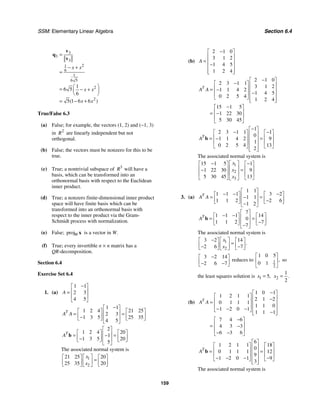
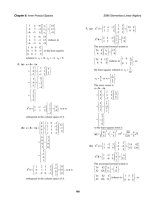
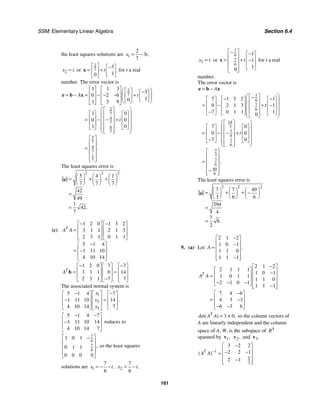
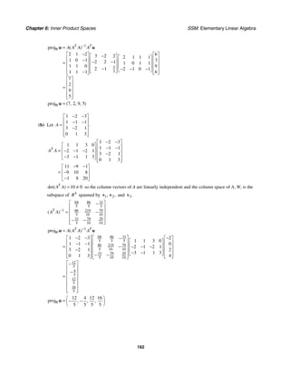
![SSM: Elementary Linear Algebra Section 6.4
163
11. (a)
1 2 0 1 3 2
3 1 1 2 1 3
2 3 1 0 1 1
5 1 4
1 11 10
4 10 14
T
A A
− −
⎡ ⎤ ⎡ ⎤
⎢ ⎥ ⎢ ⎥
=
⎢ ⎥ ⎢ ⎥
⎣ ⎦ ⎣ ⎦
−
⎡ ⎤
⎢ ⎥
= −
⎢ ⎥
⎣ ⎦
0
det( ) ,
T
A A = so A does not have linearly
independent column vectors.
(b)
2 1 3
2 0 1 4
0 1 1
1 1 0 5
1 0 2
3 1 2 3
4 5 3
21 22 20
22 27 17
20 17 23
T
A A
−
⎡ ⎤
−
⎡ ⎤ ⎢ ⎥
⎢ ⎥
= − − ⎢ ⎥
− −
⎢ ⎥ ⎢ ⎥
−
⎣ ⎦ −
⎢ ⎥
⎣ ⎦
−
⎡ ⎤
⎢ ⎥
= − −
⎢ ⎥
−
⎣ ⎦
0
det( ) ,
T
A A = so A does not have linearly
independent column vectors.
13. (a) W = the xz-plane is two-dimensional and
one basis for W is 1 2
{ , }
w w where
1 1 0 0
( , , ),
=
w 2 0 0 1
( , , ).
=
w
Thus
1 0
0 0
0 1
A
⎡ ⎤
⎢ ⎥
=
⎢ ⎥
⎣ ⎦
and
1 0 0
0 0 1
.
T
A
⎡ ⎤
= ⎢ ⎥
⎣ ⎦
1 0
1 0 0 1 0
0 0
0 0 1 0 1
0 1
T
A A
⎡ ⎤
⎡ ⎤ ⎡ ⎤
⎢ ⎥
= =
⎢ ⎥ ⎢ ⎥
⎢ ⎥
⎣ ⎦ ⎣ ⎦
⎣ ⎦
1
1 0
1 0 1 0 0
0 0
0 1 0 0 1
0 1
1 0
1 0 0
0 0
0 0 1
0 1
1 0 0
0 0 0
0 0 1
[ ] ( )
T T
P A A A A
−
=
⎡ ⎤
⎡ ⎤ ⎡ ⎤
⎢ ⎥
= ⎢ ⎥ ⎢ ⎥
⎢ ⎥ ⎣ ⎦ ⎣ ⎦
⎣ ⎦
⎡ ⎤
⎡ ⎤
⎢ ⎥
= ⎢ ⎥
⎢ ⎥ ⎣ ⎦
⎣ ⎦
⎡ ⎤
⎢ ⎥
=
⎢ ⎥
⎣ ⎦
(b) W = the yz-plane is two-dimensional and
one basis for W is 1 2
{ , }
w w where
1 0 1 0
( , , )
=
w and 2 0 0 1
( , , ).
=
w
Thus
0 0
1 0
0 1
A
⎡ ⎤
⎢ ⎥
=
⎢ ⎥
⎣ ⎦
and
0 1 0
0 0 1
.
T
A
⎡ ⎤
= ⎢ ⎥
⎣ ⎦
0 0
0 1 0 1 0
1 0
0 0 1 0 1
0 1
T
A A
⎡ ⎤
⎡ ⎤ ⎡ ⎤
⎢ ⎥
= =
⎢ ⎥ ⎢ ⎥
⎢ ⎥
⎣ ⎦ ⎣ ⎦
⎣ ⎦
1
0 0
1 0 0 1 0
1 0
0 1 0 0 1
0 1
0 0
0 1 0
1 0
0 0 1
0 1
0 0 0
0 1 0
0 0 1
[ ] ( )
T T
P A A A A
−
=
⎡ ⎤
⎡ ⎤ ⎡ ⎤
⎢ ⎥
= ⎢ ⎥ ⎢ ⎥
⎢ ⎥ ⎣ ⎦ ⎣ ⎦
⎣ ⎦
⎡ ⎤
⎡ ⎤
⎢ ⎥
= ⎢ ⎥
⎢ ⎥ ⎣ ⎦
⎣ ⎦
⎡ ⎤
⎢ ⎥
=
⎢ ⎥
⎣ ⎦
15. (a) If x = s and y = t, then a point on the plane is
(s, t, −5s + 3t) = s(1, 0, −5) + t(0, 1, 3).
1 1 0 5
( , , )
= −
w and 2 0 1 3
( , , )
=
w are a
basis for W.
(b)
1 0
0 1
5 3
,
A
⎡ ⎤
⎢ ⎥
=
⎢ ⎥
−
⎣ ⎦
1 0 5
0 1 3
,
T
A
−
⎡ ⎤
= ⎢ ⎥
⎣ ⎦
1 0
1 0 5 26 15
0 1
0 1 3 15 10
5 3
T
A A
⎡ ⎤
− −
⎡ ⎤ ⎡ ⎤
⎢ ⎥
= =
⎢ ⎥ ⎢ ⎥
−
⎢ ⎥
⎣ ⎦ ⎣ ⎦
−
⎣ ⎦
35
det( ) ,
T
A A = 1 1 10 15
15 26
35
( )
T
A A − ⎡ ⎤
= ⎢ ⎥
⎣ ⎦
1
1 0
1 10 15 1 0 5
0 1
15 26 0 1 3
35
5 3
10 15
1 1 0 5
15 26
0 1 3
35 5 3
10 15 5
1
15 26 3
35 5 3 34
[ ] ( )
T T
P A A A A
−
=
⎡ ⎤
⎛ ⎞ −
⎡ ⎤ ⎡ ⎤
⎢ ⎥
= ⎜ ⎟
⎢ ⎥ ⎢ ⎥
⎢ ⎥ ⎣ ⎦ ⎣ ⎦
⎝ ⎠
−
⎣ ⎦
⎡ ⎤
−
⎡ ⎤
⎢ ⎥
= ⎢ ⎥
⎢ ⎥ ⎣ ⎦
−
⎣ ⎦
−
⎡ ⎤
⎢ ⎥
=
⎢ ⎥
−
⎣ ⎦](https://image.slidesharecdn.com/elementary-linear-algebra-chapter1-220420115526/85/Elementary-linear-algebra-chapter-1-pdf-218-320.jpg)
![Chapter 6: Inner Product Spaces SSM: Elementary Linear Algebra
164
(c)
0 0 0
0 0 0
0 0 0
0 0
0 0
0 0
0 0 0
0 0 0
0 0 0
10 15 5
35
15 26 3
35
5 3 34
35
10 15 5
1
15 26 3
35 5 3 34
10 15 5
1
15 26 3
35
5 3 34
[ ]
x y z
x y z
x y z
x x
y y
P
z z
x y z
x y z
x y z
+ −
+ +
− + +
⎡ ⎤ ⎡ ⎤
−
⎡ ⎤
⎢ ⎥ ⎢ ⎥
⎢ ⎥
=
⎢ ⎥ ⎢ ⎥
⎢ ⎥
−
⎢ ⎥ ⎢ ⎥
⎣ ⎦
⎣ ⎦ ⎣ ⎦
+ −
⎡ ⎤
⎢ ⎥
+ +
=
⎢ ⎥
− + +
⎢ ⎥
⎣ ⎦
⎡ ⎤
⎢ ⎥
⎢ ⎥
=
⎢ ⎥
⎢ ⎥
⎢ ⎥
⎣ ⎦
The orthogonal projection is 0 0 0 0 0 0 0 0 0
2 3 15 26 3 5 3 34
7 35 35
.
, ,
x y z x y z x y z
− − + + − + +
⎛ ⎞
⎜ ⎟
⎝ ⎠
(d) The orthogonal projection of 0 1 2 4
( , , )
P − on W is
2 1 3 2 4 15 1 26 2 3 4 5 1 3 2 34 4 8 5 25
7 35 35 7 7 7
( ) ( ) ( ) ( ) ( ) ( ) ( ) ( )
.
, , , ,
− − − + − + − + − +
⎛ ⎞ ⎛ ⎞
= − −
⎜ ⎟ ⎜ ⎟
⎝ ⎠ ⎝ ⎠
The distance between 0 1 2 4
( , , )
P − and W is
2 2 2
3 35
8 5 25
1 2 4
7
7 7 7
.
d
⎛ ⎞ ⎛ ⎞
⎛ ⎞ ⎛ ⎞ ⎛ ⎞
= − + − − + =
− − −
⎜ ⎟ ⎜ ⎟ ⎜ ⎟
⎜ ⎟ ⎜ ⎟
⎝ ⎠ ⎝ ⎠ ⎝ ⎠
⎝ ⎠ ⎝ ⎠
Using Theorem 3.3.4, the distance is
2 2 2
5 1 3 2 4 15 3 35
7
35
5 3 1
( ) ( )
.
( )
− − +
= =
+ − +
17. By inspection, when t = 1, the point (t, t, t) = (1, 1, 1) is on line l. When s = 1, the point (s, 2s − 1, 1) = (1, 1, 1) is
on line m. Thus since 0,
≥
−
P Q these are the values of s and t that minimize the distance between the lines.
19. If A has linearly independent column vectors, then T
A A is invertible and the least squares solution of Ax = b is
the solution of ,
T T
A A A
=
x b but since b is orthogonal to the column space of A, ,
T
A =
b 0 so x is a solution of
.
T
A A =
x 0 Thus, x = 0 since T
A A is invertible.
21. T
A will have linearly independent column vectors, and the column space of T
A is the row space of A. Thus, the
standard matrix for the orthogonal projection of n
R onto the row space of A is
1 1
[ ] [( ) ] ( ) ( ) .
T T T T T T T T
P A A A A A AA A
− −
= =
True/False 6.4
(a) True; T
A A is an n × n matrix.
(b) False; only square matrices have inverses, but T
A A can be invertible when A is not a square matrix.
(c) True; if A is invertible, so is ,
T
A so the product T
A A is also invertible.
(d) True
(e) False; the system T T
A A A
=
x b may be consistent.
(f) True](https://image.slidesharecdn.com/elementary-linear-algebra-chapter1-220420115526/85/Elementary-linear-algebra-chapter-1-pdf-219-320.jpg)
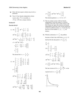
![Chapter 6: Inner Product Spaces SSM: Elementary Linear Algebra
166
True/False 6.5
(a) False; there is only a unique least squares
straight line fit if the data points do not lie on a
vertical line.
(b) True; if the points are not collinear, there is no
solution to the system.
(c) False; the sum 2 2 2
1 2 n
d d d
+ + + is minimized,
not the individual terms .
i
d
(d) True
Section 6.6
Exercise Set 6.6
1. With f(x) = 1 + x:
2
2
2
0 0
0
1 1
1 2 2
2
( ) x
a x dx x
π
π
π
π π
⎛ ⎞
= + = = +
+
⎜ ⎟
⎝ ⎠
∫
2
0
2 2
0 0
2
0
1
1
1 1
1
0
0
( )cos
cos cos
sin
k
a x kx dx
kxdx x kx dx
kx
k
π
π π
π
π
π π
π
= +
= +
= +
=
∫
∫ ∫
2
0
2 2
0 0
2
0
1
1
1 1
2
1
2
( )sin
sin sin
cos
k
b x kxdx
kx dx x kx dx
kx
k
k
k
π
π π
π
π
π π
π
= +
= +
= − −
= −
∫
∫ ∫
(a) 0 2 2 ,
a π
= + 1 2 0,
a a
= = 1 2,
b = − 2 1
b = −
Thus
1
2 2 2 2
2
1 2 2
( ) ( ) sin sin
( ) sin sin .
f x x x
x x
π
π
≈ + − −
= + − −
(b) 1 2 0
n
a a a
= = =
2
k
b
k
= − so 2
sin
sin .
k
kx
b kx
k
⎛ ⎞
= − ⎜ ⎟
⎝ ⎠
2
1 2
2
sin sin
( ) ( ) sin
x nx
f x x
n
π ⎛ ⎞
≈ + − + + +
⎜ ⎟
⎝ ⎠
3. (a) The space W of continuous functions of the
form x
a be
+ over [0, 1] is spanned by
1 1
=
v and 2 .
x
e
=
v
Let 1 1 1.
= =
g v
1
2 2
1 0
1 1
dx
= =
∫
g
1 1
2 1 0
0
1
, x x
e dx e
e
= = = −
∫
v g
2 1
2 2 1
2
1
1
1
1
1
,
( )
x
x
e
e
e e
= −
−
= −
= − +
v g
g v g
g
2
2
1 2
0
1 2 2
0
1
2 1 2
0
2
1
1 2 2 2
1
2 2 2
2
3 1
2
2 2
1
1 3
2
( )
( )
( )( )
x
x x x
x x x
e e dx
e e e ee e dx
x ex e x e e e
e e
e e
+
= − +
= − + + − +
⎛ ⎞
= − + + − +
⎜ ⎟
⎝ ⎠
= − + −
= − − −
∫
∫
g
1
g and 2
g are an orthogonal basis for W.
The least squares approximation of x is the
orthogonal projection of x on W,
1 2
1 2
2 2
1 2
proj
, ,
W
x x
x = +
g g
g g
g g
1
1 2
1 0
0
1
1
2
2
, xdx
x x
= = =
∫
g
1
2 0
1
3 1
2 2
1
3
2
( )
,
( )
x
x e e dx
x
e
e
= − +
= −
= −
∫
g
1 1
2 2
1
2
3
proj 1 1
1 1 3
1 1
1
2 1
1 1 1
2 1 1
1 1
2 1
( )
( ) ( )
( )( )
( )
x
W
x
x
x
e
x e e
e e
e e
e
e
e
e e
e
e
−
= + − +
− − −
= − − +
−
−
= − −
− −
= − +
−](https://image.slidesharecdn.com/elementary-linear-algebra-chapter1-220420115526/85/Elementary-linear-algebra-chapter-1-pdf-221-320.jpg)
![SSM: Elementary Linear Algebra Section 6.5
167
(b) Let 1 x
=
f and 2 1
proj ,
W
=
f f then the mean
square error is
2
1 2 .
−
f f Recall that
1 1 1 2
projW
− = −
f f f f and 2
f are orthogonal.
2
1 2 1 2 1 2
1 1 2 2 1 2
1 1 2
1 1 1 2
2
1 1 2
,
, ,
,
, ,
,
=
− − −
= −
− −
= −
= −
= −
f f f f f f
f f f f f f
f f f
f f f f
f f f
Now decompose 2
f in terms of 1
g and 2
g
from part (a).
2
1 2
2 1 1 1 2
1 1 1 1 2
2 2
1 2
2 2
2 1 1 1 2
1 2 2
1 2
, ,
, ,
, ,
−
= − −
= − −
f f
f g f g
f f g f g
g g
f g f g
f
g g
1
3
1
2 2
1 0
0
1
3
3
x
x dx
= = =
∫
f
Thus,
( ) ( )
2 2
1 1
2 2 2
1 2 1
2
3
1
3 1 1 3
1 1 3
3 4 2 1
1 2 2 1
12 2 1
13 1
12 2 1
( )
( )( )
( )
( )
( )
e
e e
e
e
e e
e
e
e
−
= − −
−
− − −
−
= − +
−
− + +
= +
−
+
= +
−
f f
5. (a) The space W of continuous functions of the
form 2
0 1 2
a a x a x
+ + over [−1, 1] is
spanned by 1 1,
=
v 2 ,
x
=
v and 2
3 .
x
=
v
Let 1 1 1.
= =
g v
1
2 2 1
1 1
1
1 2
dx x −
−
= = =
∫
g
1
1 2
2 1 1
1
1
0
2
, x dx x
−
−
= = =
∫
v g
2 1
2 2 1 2
2
1
,
x
= − = =
v g
g v g v
g
1
1
2 2 3
2 1
1
2
1
3
3
x dx x
−
−
= = =
∫
g
1 2
3 1 1
2
3
, x dx
−
= =
∫
v g
1
1 3 4
3 2 1
1
1
0
4
, x dx x
−
−
= = =
∫
v g
3 1 3 2
3 3 1 2
2 2
1 2
2
2 3
2
1 0
2
1
3
, ,
( )
x
x
= − −
= − −
= − +
v g v g
g v g g
g g
1 2 3
{ , , }
g g g is an orthogonal basis for W.
The least squares approximation of
1 sin x
π
=
f is the orthogonal projection of
1
f on W,
1 3
1 1 1 2
1 1 2 3
2 2 2
1 2 3
proj
,
, ,
W = + +
f g
f g f g
f g g g
g g g
1
1
1 1 1
1
1
0
sin
, cos
x dx x
π π
π
−
−
= = =
−
∫
f g
1
1 2 1
2
sin
, x xdx
π
π
−
= =
∫
f g
1 2
1 3 1
1
0
3
, sin xdx
x π
−
⎛ ⎞
= =
− +
⎜ ⎟
⎝ ⎠
∫
f g
2
1 1 3
2
3
3
proj 0 0
W x x
π
π
= + + =
f g g
(b) Let 2 1
proj ,
W
=
f f then in a clear extension
of the process in Exercise 3(b),
2
1 2
2
2 2
2 1 3
1 1 1 2
1 2 2 2
1 2 3
,
, ,
−
= − − −
f f
f g
f g f g
f
g g g
1
2 2
1 1
1
sin xdx
π
−
= =
∫
f
Thus, the mean square error is
( )
2
2
2
1 2 2 2
3
6
1 0 0 1
π
π
= − − − = −
−
f f
9. Let
1 0
0 2
,
( ) .
,
x
f x
x
π
π π
⎧
= ⎨ ≤ ≤
⎩
2
0 0 0
1 1
1
( )
a f x dx dx
π π
π π
= = =
∫ ∫](https://image.slidesharecdn.com/elementary-linear-algebra-chapter1-220420115526/85/Elementary-linear-algebra-chapter-1-pdf-222-320.jpg)
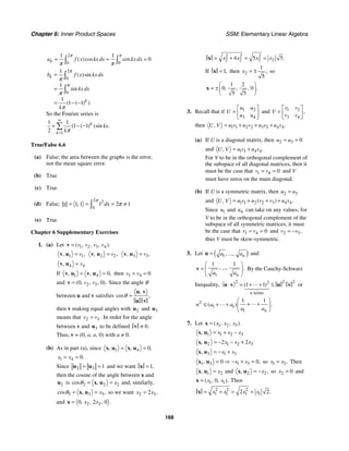
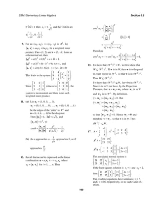
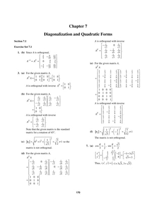
![SSM: Elementary Linear Algebra Section 7.1
171
(b) Since a rotation matrix is orthogonal,
Equation (2) gives
5
3
1
2
2 2
5 3
3 1
2
2 2
3
5
2 1
.
x
y
⎡ ⎤ ⎡ ⎤
−
−
⎡ ⎤ ⎡ ⎤
⎢ ⎥ ⎢ ⎥
= =
⎢ ⎥ ⎢ ⎥
⎢ ⎥ ⎢ ⎥
⎣ ⎦ ⎣ ⎦ +
⎣ ⎦
⎣ ⎦
Thus,
5 5
3 3 1
2 2
( , ) .
,
x y
⎛ ⎞
= − +
⎜ ⎟
⎝ ⎠
9. If 1 2 3
{ , , }
B = u u u is the standard basis for 3
,
R
and 1 2 3
{ , , }
B′ ′ ′ ′
= u u u is the rotated basis, then
the transition matrix from B′ to B is
3
1
3 3 2 2
3 1
3 3 2 2
0 0
0 1 0 0 1 0
0 0
cos sin
sin cos
P
π π
π π
⎡ ⎤
⎡ ⎤
⎢ ⎥
⎢ ⎥
= = ⎢ ⎥
⎢ ⎥
⎢ ⎥
⎢ ⎥
− −
⎢ ⎥
⎣ ⎦ ⎣ ⎦
(a) 1
3
1
2 2
3 1
2 2
5
1
2 2
5
1
2 2
0 1
0 1 0 2
5
0
3
2
3
x x
P
y y
z z
−
′
⎡ ⎤ ⎡ ⎤
⎢ ⎥ ⎢ ⎥
′ =
⎢ ⎥ ⎢ ⎥
′
⎣ ⎦ ⎣ ⎦
⎡ ⎤
− −
⎡ ⎤
⎢ ⎥
⎢ ⎥
= ⎢ ⎥
⎢ ⎥
⎢ ⎥
⎣ ⎦
⎢ ⎥
⎣ ⎦
⎡ ⎤
− −
⎢ ⎥
= ⎢ ⎥
⎢ ⎥
− +
⎣ ⎦
Thus
1 5 1 5
3 2 3
2 2 2 2
( , , ) .
, ,
x y z
⎛ ⎞
′ ′ ′ = − − − +
⎜ ⎟
⎝ ⎠
(b)
3
1
2 2
3 1
2 2
3
1
2 2
3
1
2 2
0 1
0 1 0 6
3
0
3
6
3
x x
P
y y
z z
⎡ ⎤
′
⎡ ⎤ ⎡ ⎤ ⎡ ⎤
⎢ ⎥
⎢ ⎥ ⎢ ⎥ ⎢ ⎥
′
= = ⎢ ⎥
⎢ ⎥ ⎢ ⎥ ⎢ ⎥
⎢ ⎥
′ −
⎣ ⎦ ⎣ ⎦ ⎣ ⎦
−
⎢ ⎥
⎣ ⎦
⎡ ⎤
−
⎢ ⎥
= ⎢ ⎥
⎢ ⎥
− −
⎣ ⎦
Thus
1 3 1 3
3 6 3
2 2 2 2
( , , ) .
, ,
x y z
⎛ ⎞
= − − −
⎜ ⎟
⎝ ⎠
11. (a) If 1 2 3
{ , , }
B = u u u is the standard basis for
3
R and 1 2 3
{ , , },
B′ ′ ′ ′
= u u u then
1 0
cos
[ ] ,
sin
B
θ
θ
⎡ ⎤
⎢ ⎥
′ =
⎢ ⎥
−
⎣ ⎦
u 2
0
1
0
[ ] ,
B
⎡ ⎤
⎢ ⎥
′ =
⎢ ⎥
⎣ ⎦
u and
3 0
sin
[ ] .
cos
B
θ
θ
⎡ ⎤
⎢ ⎥
′ =
⎢ ⎥
⎣ ⎦
u Thus the transition matrix
from B′ to B is
0
0 1 0
0
cos sin
,
sin cos
P
θ θ
θ θ
⎡ ⎤
⎢ ⎥
=
⎢ ⎥
−
⎣ ⎦
i.e., .
x x
P
y y
z z
′
⎡ ⎤ ⎡ ⎤
⎢ ⎥ ⎢ ⎥
′
=
⎢ ⎥ ⎢ ⎥
′
⎣ ⎦ ⎣ ⎦
Then
1
0
0 1 0
0
cos sin
.
sin cos
A P
θ θ
θ θ
−
−
⎡ ⎤
⎢ ⎥
= =
⎢ ⎥
⎣ ⎦
(b) With the same notation, 1
1
0
0
[ ] ,
B
⎡ ⎤
⎢ ⎥
′ =
⎢ ⎥
⎣ ⎦
u
2
0
[ ] ,
cos
sin
B θ
θ
⎡ ⎤
⎢ ⎥
′ =
⎢ ⎥
⎣ ⎦
u and 3
0
[ ] ,
sin
cos
B θ
θ
⎡ ⎤
⎢ ⎥
′ = −
⎢ ⎥
⎣ ⎦
u so
the transition matrix from B′ to B is
1 0 0
0
0
cos sin
sin cos
P θ θ
θ θ
⎡ ⎤
⎢ ⎥
= −
⎢ ⎥
⎣ ⎦
and
1 0 0
0
0
.
cos sin
sin cos
A θ θ
θ θ
⎡ ⎤
⎢ ⎥
=
⎢ ⎥
−
⎣ ⎦
13. Let .
a b b a
A
a b b a
+ −
⎡ ⎤
= ⎢ ⎥
− +
⎣ ⎦
Then
2 2
2 2
2 0
0 2
( )
,
( )
T a b
A A
a b
⎡ ⎤
+
= ⎢ ⎥
+
⎢ ⎥
⎣ ⎦
so a and b
must satisfy 2 2 1
2
.
a b
+ =
17. The row vectors of an orthogonal matrix are an
orthonormal set.
2 2
2 2 2
1
1 1
1
2 2
a a
⎛ ⎞ ⎛ ⎞
−
= + + = +
⎜ ⎟ ⎜ ⎟
⎝ ⎠ ⎝ ⎠
r
Thus a = 0.
2 2
2 2 2
2
1 1 2
6
6 6
b b
⎛ ⎞ ⎛ ⎞
= + + = +
⎜ ⎟ ⎜ ⎟
⎝ ⎠ ⎝ ⎠
r
Thus
2
6
.
b = ±
2 2
2 2 2
3
1 1 2
3
3 3
c c
⎛ ⎞ ⎛ ⎞
= + + = +
⎜ ⎟ ⎜ ⎟
⎝ ⎠ ⎝ ⎠
r](https://image.slidesharecdn.com/elementary-linear-algebra-chapter1-220420115526/85/Elementary-linear-algebra-chapter-1-pdf-226-320.jpg)
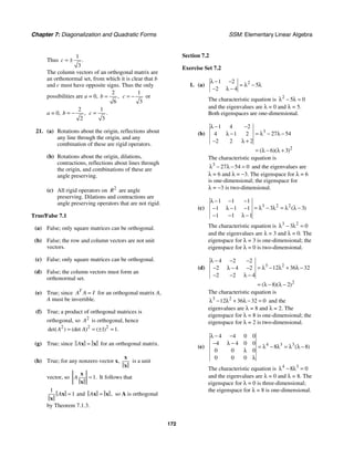
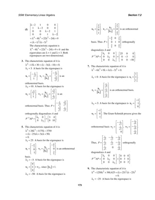
![Chapter 7: Diagonalization and Quadratic Forms SSM: Elementary Linear Algebra
174
4
3
1
1
0
0
,
⎡ ⎤
−
⎢ ⎥
⎢ ⎥
=
⎢ ⎥
⎢ ⎥
⎣ ⎦
x 4
2
3
0
0
1
.
⎡ ⎤
⎢ ⎥
⎢ ⎥
=
−
⎢ ⎥
⎢ ⎥
⎣ ⎦
x The Gram-Schmidt
process gives the orthonormal basis
4
5
3
5
1
0
0
,
⎡ ⎤
−
⎢ ⎥
⎢ ⎥
=
⎢ ⎥
⎢ ⎥
⎢ ⎥
⎣ ⎦
v
4
2
5
3
5
0
0
.
⎡ ⎤
⎢ ⎥
⎢ ⎥
= −
⎢ ⎥
⎢ ⎥
⎢ ⎥
⎣ ⎦
v
2 25:
λ = A basis for the eigenspace is
3
4
3
1
0
0
,
⎡ ⎤
⎢ ⎥
⎢ ⎥
=
⎢ ⎥
⎢ ⎥
⎣ ⎦
x 3
4
4
0
0
1
.
⎡ ⎤
⎢ ⎥
⎢ ⎥
=
⎢ ⎥
⎢ ⎥
⎣ ⎦
x The Gram-Schmidt
process gives the orthonormal basis
3
5
4
5
3
0
0
,
⎡ ⎤
⎢ ⎥
⎢ ⎥
=
⎢ ⎥
⎢ ⎥
⎢ ⎥
⎣ ⎦
v
3
4
5
4
5
0
0
.
⎡ ⎤
⎢ ⎥
⎢ ⎥
=
⎢ ⎥
⎢ ⎥
⎢ ⎥
⎣ ⎦
v Thus,
3
4
5 5
3 4
5 5
1 2 3 4 3
4
5 5
3 4
5 5
0 0
0 0
0 0
0 0
[ ]
P
⎡ ⎤
−
⎢ ⎥
⎢ ⎥
= = ⎢ ⎥
−
⎢ ⎥
⎢ ⎥
⎢ ⎥
⎣ ⎦
v v v v
orthogonally diagonalizes A and
1
1 2
1
2
0 0 0
0 0 0
0 0 0
0 0 0
25 0 0 0
0 25 0 0
0 0 25 0
0 0 0 25
.
P AP
−
λ
⎡ ⎤
⎢ ⎥
λ
= ⎢ ⎥
λ
⎢ ⎥
⎢ ⎥
λ
⎣ ⎦
−
⎡ ⎤
⎢ ⎥
= ⎢ ⎥
−
⎢ ⎥
⎢ ⎥
⎣ ⎦
15. No, a non-symmetric matrix A can have
eigenvalues that are real numbers. For instance,
the eigenvalues of the matrix
3 0
8 1
⎡ ⎤
⎢ ⎥
−
⎣ ⎦
are 3 and
−1.
17. If A is an orthogonal matrix then its eigenvalues
have absolute value 1, but may be complex.
Since the eigenvalues of a symmetric matrix
must be real numbers, the only possible
eigenvalues for an orthogonal symmetric matrix
are 1 and −1.
19. Yes; to diagonalize A, follow the steps on page
399. The Gram-Schmidt process will ensure that
columns of P corresponding to the same
eigenvalue are an orthonormal set. Since
eigenvectors from distinct eigenvalues are
orthogonal, this means that P will be an
orthogonal matrix. Then since A is orthogonally
diagonalizable, it must be symmetric.
True/False 7.2
(a) True; for any square matrix A, both T
AA and
T
A A are symmetric, hence orthogonally
diagonalizable.
(b) True; since 1
v and 2
v are from distinct
eigenspaces of a symmetric matrix, they are
orthogonal, so
2
1 2 1 2 1 2
1 1 1 2 2 2
2 2
1 2
2
0
,
, , ,
.
=
+ + +
= + +
= + +
v v v v v v
v v v v v v
v v
(c) False; an orthogonal matrix is not necessarily
symmetric.
(d) True; 1 1 1 1
( )
P AP P A P
− − − −
= since 1
P−
and
1
A−
both exist and since 1
P AP
−
is diagonal, so
is 1 1
( ) .
P AP
− −
(e) True; since A =
x x for an orthogonal matrix.
(f) True; if A is an n × n orthogonally
diagonalizable matrix, then A has an
orthonormal set of n eigenvectors, which form a
basis for .
n
R](https://image.slidesharecdn.com/elementary-linear-algebra-chapter1-220420115526/85/Elementary-linear-algebra-chapter-1-pdf-229-320.jpg)
![SSM: Elementary Linear Algebra Section 7.3
175
(g) True; if A is orthogonally diagonalizable, then A
must be symmetric, so the eigenvalues of A will
all be real numbers.
Section 7.3
Exercise Set 7.3
1. (a) 2 2 1
1 2 1 2
2
3 0
3 7
0 7
[ ]
x
x x x x
x
⎡ ⎤
⎡ ⎤
+ = ⎢ ⎥
⎢ ⎥
⎣ ⎦ ⎣ ⎦
(b) 2 2 1
1 2 1 2 1 2
2
4 3
4 9 6
3 9
[ ]
x
x x x x x x
x
− ⎡ ⎤
⎡ ⎤
− − = ⎢ ⎥
⎢ ⎥
− −
⎣ ⎦ ⎣ ⎦
(c) 2 2 2
1 2 3 1 2 1 3 2 3
1
1
2 2
1 2 3
1
3
2
9 4 6 8
9 3 4
3 1
4 4
[ ]
x x x x x x x x x
x
x
x x x
x
− + + − +
−
⎡ ⎤ ⎡ ⎤
⎢ ⎥ ⎢ ⎥
−
= ⎢ ⎥ ⎢ ⎥
⎢ ⎥
− ⎣ ⎦
⎣ ⎦
3. 2 2
2 3
2 5 6
3 5
[ ]
x
x y x y xy
y
−
⎡ ⎤ ⎡ ⎤
= + −
⎢ ⎥ ⎢ ⎥
−
⎣ ⎦ ⎣ ⎦
5. 1
1 2
2
2 1
1 2
[ ]
T x
Q A x x
x
− ⎡ ⎤
⎡ ⎤
= = ⎢ ⎥
⎢ ⎥
−
⎣ ⎦ ⎣ ⎦
x x
The characteristic equation of A is
2
4 3 3 1 0
( )( ) ,
λ − λ + = λ − λ − = so the
eigenvalues are 3 1
, .
λ = Orthonormal bases for
the eigenspaces are λ = 3:
1
2
1
2
;
⎡ ⎤
⎢ ⎥
⎢ ⎥
−
⎣ ⎦
λ = 1:
1
2
1
2
.
⎡ ⎤
⎢ ⎥
⎢ ⎥
⎣ ⎦
For
1 1
2 2
1 1
2 2
,
P
⎡ ⎤
⎢ ⎥
=
⎢ ⎥
−
⎣ ⎦
let x = Py, then
1
1 2
2
3 0
0 1
( ) [ ]
T T T y
A P AP y y
y
⎡ ⎤
⎡ ⎤
= = ⎢ ⎥
⎢ ⎥
⎣ ⎦ ⎣ ⎦
x x y y
and 2 2
1 2
3 .
Q y y
= +
7.
1
2
1 2 3
3
3 2 0
2 4 2
0 2 5
[ ]
T
x
x
Q A x x x
x
⎡ ⎤
⎡ ⎤
⎢ ⎥
⎢ ⎥
= = −
⎢ ⎥
⎢ ⎥
−
⎣ ⎦ ⎣ ⎦
x x
The characteristic equation of A is
3 2
12 39 28 1 4 7 0
( )( )( ) ,
λ − λ + λ − = λ − λ − λ − =
so the eigenvalues are λ = 1, 4, 7. Orthonormal
bases for the eigenspaces are λ = 1:
2
3
2
3
1
3
;
⎡ ⎤
−
⎢ ⎥
⎢ ⎥
⎢ ⎥
⎢ ⎥
⎣ ⎦
λ = 4:
2
3
1
3
2
3
;
⎡ ⎤
⎢ ⎥
⎢ ⎥
⎢ ⎥
⎢ ⎥
⎣ ⎦
λ = 7:
1
3
2
3
2
3
.
⎡ ⎤
⎢ ⎥
⎢ ⎥
⎢ ⎥
−
⎢ ⎥
⎣ ⎦
For
2 2 1
3 3 3
2 1 2
3 3 3
1 2 2
3 3 3
,
P
⎡ ⎤
−
⎢ ⎥
= ⎢ ⎥
⎢ ⎥
−
⎢ ⎥
⎣ ⎦
let x = Py, then
1
2
1 2 3
3
1 0 0
0 4 0
0 0 7
( )
[ ]
T T T
A P AP
y
y
y y y
y
=
⎡ ⎤
⎡ ⎤
⎢ ⎥
⎢ ⎥
=
⎢ ⎥
⎢ ⎥
⎣ ⎦ ⎣ ⎦
x x y y
and
2 2 2
1 2 3
4 7 .
Q y y y
= + +
9. (a) 2
2 6 2 0
x xy x y
+ + − + = can be written as
2 2
2 0 6 2 0
( )
x y xy x y
+ + + − + = or
1
2
1
2
2
1 6 2 0
0
[ ] [ ] .
x x
x y
y y
⎡ ⎤ ⎡ ⎤ ⎡ ⎤
⎢ ⎥ + − + =
⎢ ⎥ ⎢ ⎥
⎣ ⎦ ⎣ ⎦
⎢ ⎥
⎣ ⎦
(b) 2
7 8 5 0
y x y
+ − − = can be written as
2 2
0 0 7 8 5 0
( )
x y xy x y
+ + + − − = or
0 0
7 8 5 0
0 1
[ ] [ ] .
x x
x y
y y
⎡ ⎤ ⎡ ⎤ ⎡ ⎤
+ − − =
⎢ ⎥ ⎢ ⎥ ⎢ ⎥
⎣ ⎦ ⎣ ⎦ ⎣ ⎦
11. (a) 2 2
2 5 20
x y
+ = is
2 2
1
10 4
x y
+ = which is the
equation of an ellipse.
(b) 2 2
8 0
x y
− − = is 2 2
8
x y
− = or
2 2
1
8 8
x y
− = which is the equation of a
hyperbola.
(c) 2
7 2 0
y x
− = is 2
7
2
x y
= which is the
equation of a parabola.
(d) 2 2
25 0
x y
+ − = is 2 2
25
x y
+ = which is
the equation of a circle.](https://image.slidesharecdn.com/elementary-linear-algebra-chapter1-220420115526/85/Elementary-linear-algebra-chapter-1-pdf-230-320.jpg)
![Chapter 7: Diagonalization and Quadratic Forms SSM: Elementary Linear Algebra
176
13. The equation can be written in matrix form as
8
T
A = −
x x where
2 2
2 1
.
A
−
⎡ ⎤
= ⎢ ⎥
− −
⎣ ⎦
The
eigenvalues of A are 1 3
λ = and 2 2,
λ = − with
corresponding eigenvectors 1
2
1
⎡ ⎤
= ⎢ ⎥
−
⎣ ⎦
v and
2
1
2
⎡ ⎤
= ⎢ ⎥
⎣ ⎦
v respectively. Thus the matrix
2 1
5 5
1 2
5 5
P
⎡ ⎤
⎢ ⎥
=
⎢ ⎥
−
⎣ ⎦
orthogonally diagonalizes A.
Note that det(P) = 1, so P is a rotation matrix.
The equation of the conic in the rotated
-coordinate
x y
′ ′ system is
3 0
8
0 2
[ ]
x
x y
y
′
⎡ ⎤ ⎡ ⎤
′ ′ = −
⎢ ⎥ ⎢ ⎥
′
−
⎣ ⎦ ⎣ ⎦
which can be written
as 2 2
2 3 8;
y x
′ ′
− = thus the conic is a hyperbola.
The angle through which the axes have been
rotated is 1 1
26 6
2
tan . .
θ − ⎛ ⎞
= ≈ − °
−
⎜ ⎟
⎝ ⎠
15. The equation can be written in matrix form as
15
T
A =
x x where
11 12
12 4
.
A
⎡ ⎤
= ⎢ ⎥
⎣ ⎦
The
eigenvalues of A are 1 20
λ = and 2 5,
λ = − with
corresponding eigenvectors 1
4
3
⎡ ⎤
= ⎢ ⎥
⎣ ⎦
v and
2
3
4
−
⎡ ⎤
= ⎢ ⎥
⎣ ⎦
v respectively. Thus the matrix
3
4
5 5
3 4
5 5
P
⎡ ⎤
−
⎢ ⎥
=
⎢ ⎥
⎣ ⎦
orthogonally diagonalizes A. Note
that det(P) = 1, so P is a rotation matrix. The
equation of the conic in the rotated
-coordinate
x y
′ ′ system is
20 0
15
0 5
[ ]
x
x y
y
′
⎡ ⎤ ⎡ ⎤
′ ′ =
⎢ ⎥ ⎢ ⎥
′
−
⎣ ⎦ ⎣ ⎦
which we can write
as 2 2
4 3;
x y
′ ′
− = thus the conic is a hyperbola.
The angle through which the axes have been
rotated is 1 3
6 9
4
tan . .
θ − ⎛ ⎞
= ≈ 3 °
⎜ ⎟
⎝ ⎠
17. (a) The eigenvalues of
1 0
0 2
⎡ ⎤
⎢ ⎥
⎣ ⎦
are λ = 1 and
λ = 2, so the matrix is positive definite.
(b) The eigenvalues of
1 0
0 2
−
⎡ ⎤
⎢ ⎥
−
⎣ ⎦
are λ = −1
and λ = −2, so the matrix is negative
definite.
(c) The eigenvalues of
1 0
0 2
−
⎡ ⎤
⎢ ⎥
⎣ ⎦
are λ = −1 and
λ = 2, so the matrix is indefinite.
(d) The eigenvalues of
1 0
0 0
⎡ ⎤
⎢ ⎥
⎣ ⎦
are λ = 1 and
λ = 0, so the matrix is positive semidefinite.
(e) The eigenvalues of
0 0
0 2
⎡ ⎤
⎢ ⎥
−
⎣ ⎦
are λ = 0 and
λ = −2, so the matrix is negative
semidefinite.
19. We have 2 2
1 2 0
Q x x
= + for 1 2 0 0
( , ) ( , );
x x ≠
thus Q is positive definite.
21. We have 2
1 2 0
( )
Q x x
= − for 1 2
x x
≠ and
Q = 0 for 1 2;
x x
= thus Q is positive
semidefinite.
23. We have 2 2
1 2 0
x x
− for 1 0,
x ≠ 2 0
x = and
Q 0 for 1 0,
x = 2 0;
x ≠ thus Q is indefinite.
25. (a) The eigenvalues of the matrix
5 2
2 5
A
−
⎡ ⎤
= ⎢ ⎥
−
⎣ ⎦
are λ = 3 and λ = 7; thus A is
positive definite. Since 5 5
= and
5 2
21
2 5
−
=
−
are positive, we reach the
same conclusion using Theorem 7.3.4.
(b) The eigenvalues of
2 1 0
1 2 0
0 0 5
A
−
⎡ ⎤
⎢ ⎥
= −
⎢ ⎥
⎣ ⎦
are
λ = 1, λ = 3, and λ = 5; thus A is positive
definite. The determinants of the principal
submatrices are 2 2,
=
2 1
3
1 2
,
−
=
−
and
2 1 0
15
1 2 0
0 0 5
;
−
=
− thus we reach the same
conclusion using Theorem 7.3.4.](https://image.slidesharecdn.com/elementary-linear-algebra-chapter1-220420115526/85/Elementary-linear-algebra-chapter-1-pdf-231-320.jpg)
![SSM: Elementary Linear Algebra Section 7.3
177
27. The quadratic form 2 2 2
1 2 3 1 2 1 3 2 3
5 4 2 2
Q x x kx x x x x x x
= + + + − − can be expressed in matrix notation as T
Q A
= x x
where
5 2 1
2 1 1
1 1
.
A
k
−
⎡ ⎤
⎢ ⎥
= −
⎢ ⎥
− −
⎣ ⎦
The determinants of the principal submatrices of A are 5 5,
=
5 2
1
2 1
,
= and
5 2 1
2
2 1 1
1 1
.
k
k
−
= −
−
− −
Thus Q is positive definite if and only if k 2.
31. (a) For each i = 1, ..., n we have
2 2 2
2
2
2
1
1
2
2
2
1 1 1
1
2
1 1
2
2 1
2
( )
.
i i i
n
n
j
i i j
j
j
n n n
n
j j k
i i j
j j k j
j
x x x x x x
x
x x x
n n
x x x
x x x
n n
=
=
= = = +
=
− = − +
⎛ ⎞
⎜ ⎟
= − +
⎜ ⎟
⎝ ⎠
⎛ ⎞
+
⎜ ⎟
= − +
⎜ ⎟
⎝ ⎠
∑
∑
∑ ∑ ∑
∑
Thus in the quadratic form 2 2 2 2
1 2
1
1
[( ) ( ) ( ) ]
x n
s x x x x x x
n
= − + − + + −
−
the coefficient of 2
i
x is
2
2 1
1 1
1
1
,
n
n
n n
n
⎡ ⎤
− + =
⎢ ⎥
− ⎣ ⎦
and the coefficient of i j
x x for i ≠ j is 2
2 2 2
1 2
1 1
.
( )
n
n n
n n n
n
⎡ ⎤
− − + = −
⎢ ⎥
− −
⎣ ⎦
It follows
that 2 T
x
s A
= x x where
1 1 1
1 1
1 1 1
1 1
1 1 1
1 1
( ) ( )
( ) ( )
( ) ( )
.
n n n n n
n n n n n
n n n n n
A
− −
− −
− −
⎡ ⎤
− −
⎢ ⎥
⎢ ⎥
− −
= ⎢ ⎥
⎢ ⎥
⎢ ⎥
− −
⎢ ⎥
⎣ ⎦
# # % #
(b) We have 2 2 2 2
1 2
1
0
1
[( ) ( ) ( ) ] ,
x n
s x x x x x x
n
= − + − + + − ≥
−
and 2
0
x
s = if and only if 1 ,
x x
=
2 , ..., ,
n
x x x x
= = i.e., if and only if 1 2 .
n
x x x
= = =
Thus 2
x
s is a positive semidefinite form.
33. The eigenvalues of A must be positive and equal to each other. That is, A must have a positive eigenvalue of
multiplicity 2.
True/False 7.3
(a) True
(b) False; because of the term 1 2 3
4 .
x x x
(c) True; 2 2 2
1 2 1 1 2 2
3 6 9
( ) .
x x x x x x
− = − +
(d) True; none of the eigenvalues will be 0.
(e) False; a symmetric matrix can be positive semidefinite or negative semidefinite.
(f) True
(g) True; 2 2 2
1 2 n
x x x
⋅ = + + +
x x](https://image.slidesharecdn.com/elementary-linear-algebra-chapter1-220420115526/85/Elementary-linear-algebra-chapter-1-pdf-232-320.jpg)
![Chapter 7: Diagonalization and Quadratic Forms SSM: Elementary Linear Algebra
178
(h) True
(i) False; this is only true for symmetric matrices.
(j) True
(k) False; there will be no cross product terms if
ij ji
a a
= − for all i ≠ j.
(l) False; if c 0, T
A c
=
x x has no graph.
Section 7.4
Exercise Set 7.4
1. The quadratic form 2 2
5x y
− can be written in
matrix notation as T
A
x x where
5 0
0 1
.
A
⎡ ⎤
= ⎢ ⎥
−
⎣ ⎦
The eigenvalues of A are 1 5
λ = and 2 1,
λ = −
with corresponding eigenvectors 1
1
0
⎡ ⎤
= ⎢ ⎥
⎣ ⎦
v and
2
0
1
.
⎡ ⎤
= ⎢ ⎥
⎣ ⎦
v Thus the constrained maximum is 5
occurring at 1 0
( , ) ( , ),
x y = ± and the constrained
minimum is −1 occurring at 0 1
( , ) ( , ).
x y = ±
3. The quadratic form 2 2
3 7
x y
+ can be written in
matrix notation as T
A
x x where
3 0
0 7
.
A
⎡ ⎤
= ⎢ ⎥
⎣ ⎦
The eigenvalues of A are 1 7
λ = and 2 3,
λ =
with corresponding unit eigenvectors 1
0
1
⎡ ⎤
= ⎢ ⎥
⎣ ⎦
v
and 2
1
0
.
⎡ ⎤
= ⎢ ⎥
⎣ ⎦
v Thus the constrained maximum is
7 occurring at (x, y) = (0, ±1), and the
constrained minimum is 3 occurring at
(x, y) = (±1, 0).
5. The quadratic form 2 2 2
9 4 3
x y z
+ + can be
expressed as T
A
x x where
9 0 0
0 4 0
0 0 3
.
A
⎡ ⎤
⎢ ⎥
=
⎢ ⎥
⎣ ⎦
The
eigenvalues of A are 1 9,
λ = 2 4,
λ = 3 3,
λ =
with corresponding eigenvectors 1
1
0
0
,
⎡ ⎤
⎢ ⎥
=
⎢ ⎥
⎣ ⎦
v
2
0
1
0
,
⎡ ⎤
⎢ ⎥
=
⎢ ⎥
⎣ ⎦
v 3
0
0
1
.
⎡ ⎤
⎢ ⎥
=
⎢ ⎥
⎣ ⎦
v Thus the constrained
maximum is 9 occurring at (x, y, z) = (±1, 0, 0),
and the constrained minimum is 3 occurring at
(x, y, z) = (0, 0, ±1).
7. Rewrite the constraint as
2
2
1
2 2
,
y
x ⎛ ⎞
⎛ ⎞
+ =
⎜ ⎟ ⎜ ⎟
⎝ ⎠ ⎝ ⎠
then let 1
2
x x
= and 1
2 .
y y
= The problem is
now to maximize 1 1
2 2
z xy x y
= = subject to
2 2
1 1 1.
x y
+ = Write
1
1 1
1
0 2
2 0
[ ] .
T x
z A x y
y
⎡ ⎤ ⎡ ⎤
= = ⎢ ⎥ ⎢ ⎥
⎣ ⎦
⎣ ⎦
x x
Since ( )( )
2
2
2 2 2
2
,
λ −
= λ − = λ + λ −
− λ
the largest eigenvalue of A is 2, with
corresponding positive unit eigenvector
1
2
1
2
.
⎡ ⎤
⎢ ⎥
⎢ ⎥
⎣ ⎦
Thus the maximum value is
1 1
2 2 2
2 2
z
⎛ ⎞⎛ ⎞
= =
⎜ ⎟⎜ ⎟
⎝ ⎠⎝ ⎠
occurs when
1
2 2,
x x
= = 1
2 1
y y
= = or 2,
x = −
y = −1. The smallest eigenvalue of A is 2,
−
with corresponding unit eigenvectors
1
2
1
2
.
⎡ ⎤
−
⎢ ⎥
±
⎢ ⎥
⎣ ⎦
Thus the minimum value is 2
z = − which
occurs at ( )
2 1
( , ) ,
x y = − and ( )
2 1 .
, −
9.
y
5
x
5
(0, 1)
(1, 0)
(0, –1)
(–1, 0)
2 2
5 5
x y
− =
2 2
5 1
x y
− = −
2 2
1
x y
+ =
13. The first partial derivatives of f are
2
3 3
( , )
x
f x y x y
= − and 2
3 3
( , ) .
y
f x y x y
= − −
To find the critical points we set x
f and y
f](https://image.slidesharecdn.com/elementary-linear-algebra-chapter1-220420115526/85/Elementary-linear-algebra-chapter-1-pdf-233-320.jpg)
![SSM: Elementary Linear Algebra Section 7.5
179
equal to zero. This yields the equations 2
y x
=
and 2
.
x y
= − From this we conclude that
4
y y
= and so y = 0 or y = 1. The corresponding
values of x are x = 0 and x = −1 respectively.
Thus there are two critical points: (0, 0) and
(−1, 1).
The Hessian matrix is
6 3
3 6
( , ) ( , )
( , ) .
( , ) ( , )
xx xy
yx yy
f x y f x y x
H x y
f x y f x y y
⎡ ⎤ −
⎡ ⎤
= =
⎢ ⎥ ⎢ ⎥
− −
⎣ ⎦
⎣ ⎦
The eigenvalues of
0 3
0 0
3 0
( , )
H
−
⎡ ⎤
= ⎢ ⎥
−
⎣ ⎦
are
λ = ±3; this matrix is indefinite and so f has a
saddle point at (0, 0). The eigenvalues of
6 3
1 1
3 6
( , )
H
− −
⎡ ⎤
− = ⎢ ⎥
− −
⎣ ⎦
are λ = −3 and
λ = −9; this matrix is negative definite and so f
has a relative maximum at (−1, 1).
15. The first partial derivatives of f are
2 2
( , )
x
f x y x xy
= − and 2
4
( , ) .
y
f x y y x
= − To
find the critical points we set x
f and y
f equal
to zero. This yields the equations 2x(1 − y) = 0
and 2
1
4
.
y x
= From the first, we conclude that
x = 0 or y = 1. Thus there are three critical
points: (0, 0), (2, 1), and (−2, 1).
The Hessian matrix is
2 2 2
2 4
( , ) ( , )
( , )
( , ) ( , )
.
xx xy
yx yy
f x y f x y
H x y
f x y f x y
y x
x
⎡ ⎤
= ⎢ ⎥
⎣ ⎦
− −
⎡ ⎤
= ⎢ ⎥
−
⎣ ⎦
The eigenvalues of the matrix
2 0
0 0
0 4
( , )
H
⎡ ⎤
= ⎢ ⎥
⎣ ⎦
are λ = 2 and λ = 4; this matrix is positive
definite and so f has a relative minimum at (0, 0).
The eigenvalues of
0 4
2 1
4 4
( , )
H
−
⎡ ⎤
= ⎢ ⎥
−
⎣ ⎦
are
2 2 5.
λ = ± One of these is positive and one is
negative; thus this matrix is indefinite and f has a
saddle point at (2, 1). Similarly, the eigenvalues
of
0 4
2 1
4 4
( , )
H
⎡ ⎤
− = ⎢ ⎥
⎣ ⎦
are 2 2 5;
λ = ± thus f
has a saddle point at (−2, 1).
17. The problem is to maximize z = 4xy subject to
2 2
25 25,
x y
+ = or
2 2
1
5 1
.
x y
⎛ ⎞ ⎛ ⎞
+ =
⎜ ⎟
⎜ ⎟
⎝ ⎠
⎝ ⎠
Let
1
5
x x
= and 1,
y y
= so that the problem is to
maximize 1 1
20
z x y
= subject to 1 1 1.
( , )
x y =
Write 1
1 1
1
0 10
10 0
[ ] .
T x
z A x y
y
⎡ ⎤
⎡ ⎤
= = ⎢ ⎥
⎢ ⎥
⎣ ⎦ ⎣ ⎦
x x
2
10
100 10 10
10
( )( ).
λ −
= λ − = λ + λ −
− λ
The largest eigenvalue of A is λ = 10 which has
positive unit eigenvector
1
2
1
2
.
⎡ ⎤
⎢ ⎥
⎢ ⎥
⎣ ⎦
Thus the
maximum value of
1 1
20 10
2 2
z
⎛ ⎞⎛ ⎞
= =
⎜ ⎟⎜ ⎟
⎝ ⎠⎝ ⎠
which occurs when 1
5
5
2
x x
= = and
1
1
2
,
y y
= = which are the corner points of the
rectangle.
21. If x is a unit eigenvector corresponding to λ,
then 1
( ) ( ) ( ) ( ) .
T T T
q A
= = λ = λ = λ = λ
x x x x x x x
True/False 7.4
(a) False; if the only critical point of the quadratic
form is a saddle point, then it will have neither a
maximum nor a minimum value.
(b) True
(c) True
(d) False; the Hessian form of the second derivative
test is inconclusive.
(e) True; if det(A) 0, then A will have negative
eigenvalues.
Section 7.5
Exercise Set 7.5
1.
2 4 5
1 3 0
*
i i
A
i i
− −
⎡ ⎤
= ⎢ ⎥
+ −
⎣ ⎦](https://image.slidesharecdn.com/elementary-linear-algebra-chapter1-220420115526/85/Elementary-linear-algebra-chapter-1-pdf-234-320.jpg)
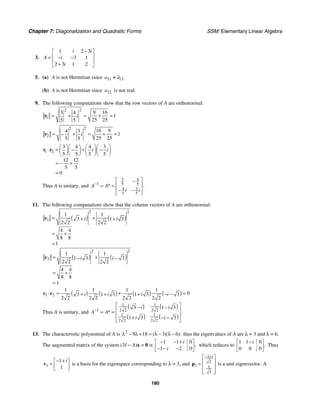
![SSM: Elementary Linear Algebra Section 7.5
181
similar computation shows that
1
6
2 2
6
i
−
⎡ ⎤
⎢ ⎥
=
⎢ ⎥
⎢ ⎥
⎣ ⎦
p is a unit eigenvector corresponding to λ = 6. The vectors 1
p and 2
p
are orthogonal, and the unitary matrix 1 2
[ ]
P = p p diagonalizes the matrix A:
P*AP
1 1 1
1
3 3 3 6
1 1 2
2
3 6
6 6
4 1
1 5
3 0
0 6
i i i
i
i
i
− − − + −
+
⎡ ⎤ ⎡ ⎤
−
⎡ ⎤
⎢ ⎥ ⎢ ⎥
= ⎢ ⎥
⎢ ⎥ ⎢ ⎥
+
⎣ ⎦
⎢ ⎥
⎢ ⎥ ⎣ ⎦
⎣ ⎦
⎡ ⎤
= ⎢ ⎥
⎣ ⎦
15. The characteristic polynomial of A is 2
10 16 2 8
( )( );
λ − λ + = λ − λ − thus the eigenvalues of A are λ = 2 and λ = 8.
The augmented matrix of the system (2I − A)x = 0 is
4 2 2 0
2 2 2 0
,
i
i
− − −
⎡ ⎤
⎢ ⎥
− + −
⎣ ⎦
which reduces to
2 1 0
0 0 0
.
i
+
⎡ ⎤
⎢ ⎥
⎣ ⎦
Thus 1
1
2
i
− −
⎡ ⎤
= ⎢ ⎥
⎣ ⎦
v is a basis for the eigenspace corresponding to λ = 2, and
1
6
1 2
6
i
− −
⎡ ⎤
⎢ ⎥
=
⎢ ⎥
⎢ ⎥
⎣ ⎦
p is a unit eigenvector. A
similar computation shows that
1
3
2 1
3
i
+
⎡ ⎤
⎢ ⎥
=
⎢ ⎥
⎢ ⎥
⎣ ⎦
p is a unit eigenvector corresponding to λ = 8. The vectors 1
p and 2
p
are orthogonal, and the unitary matrix 1 2
[ ]
P = p p diagonalizes the matrix A:
P*AP
1 1 1
2
6 6 6 3
1 2 1
1
6 3
3 3
6 2 2
2 2 4
2 0
0 8
i i i
i
i
i
− + − − +
−
⎡ ⎤ ⎡ ⎤
+
⎡ ⎤
⎢ ⎥ ⎢ ⎥
= ⎢ ⎥
⎢ ⎥ ⎢ ⎥
−
⎣ ⎦
⎢ ⎥
⎢ ⎥ ⎣ ⎦
⎣ ⎦
⎡ ⎤
= ⎢ ⎥
⎣ ⎦
17. The characteristic polynomial of A is 2
5 2 2 1 5
( )( ) ( )( )( );
λ − λ + λ − = λ + λ − λ − thus the eigenvalues of A are
1 2,
λ = − 2 1,
λ = and 3 5.
λ = The augmented matrix of the system (−2I − A)x = 0 is
7 0 0 0
0 1 1 0
0 1 2 0
,
i
i
−
⎡ ⎤
⎢ ⎥
− −
⎢ ⎥
+ −
⎣ ⎦
which can be reduced to
1 0 0 0
0 1 1 0
0 0 0 0
.
i
⎡ ⎤
⎢ ⎥
− +
⎢ ⎥
⎣ ⎦
Thus 1
0
1
1
i
⎡ ⎤
⎢ ⎥
= −
⎢ ⎥
⎣ ⎦
v is a basis for the eigenspace corresponding to
1 2,
λ = − and
1
3
1
1
3
0
i
−
⎡ ⎤
⎢ ⎥
= ⎢ ⎥
⎢ ⎥
⎢ ⎥
⎣ ⎦
p is a unit eigenvector. Similar computations show that
1
6
2
2
6
0
i
− +
⎡ ⎤
⎢ ⎥
= ⎢ ⎥
⎢ ⎥
⎢ ⎥
⎣ ⎦
p is a unit eigenvector
corresponding to 2 1,
λ = and 3
1
0
0
⎡ ⎤
⎢ ⎥
=
⎢ ⎥
⎣ ⎦
p is a unit eigenvector corresponding to 3 5.
λ = The vectors 1 2 3
{ , , }
p p p
form an orthogonal set, and the unitary matrix [ ]
1 2 3
P = p p p diagonalizes the matrix A:](https://image.slidesharecdn.com/elementary-linear-algebra-chapter1-220420115526/85/Elementary-linear-algebra-chapter-1-pdf-236-320.jpg)
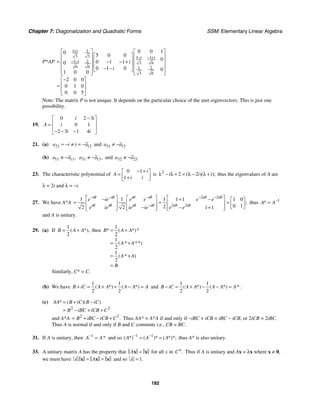
![SSM: Elementary Linear Algebra Chapter 7 Supplementary Exercises
183
35. If H = I − 2uu*, then
H* = (I − 2uu*)* = I* − 2u**u*= I − 2uu* = H;
thus H is Hermitian.
2
2 2
2 2 4
4 4
* ( *)( *)
* * * *
* *
HH I I
I
I
I
= − −
= − − +
= − +
=
uu uu
uu uu uu uu
uu u u u
and so H is unitary.
37.
1
2 2
1
2 2
i
i
A
⎡ ⎤
−
⎢ ⎥
=
⎢ ⎥
−
⎣ ⎦
is both Hermitian and unitary.
39. If P = uu*, then
( *) ( ) ( ) ( ) .
T T
P = = = = ⋅
x uu x uu x u u x x u u Thus
multiplication of x by P corresponds to
2
u
times the orthogonal projection of x onto
W = span{u}. If 1,
=
u then multiplication of x
by H = I − 2uu* corresponds to reflection of x
about the hyperplane .
⊥
u
True/False 7.5
(a) False; .
i i
≠
(b) False; for 1 2 6 3
i i i
⎡ ⎤
−
=
⎣ ⎦
r and
2 6 3
0 ,
i i
⎡ ⎤
−
=
⎣ ⎦
r
1 2
2 2
0
2 6 3
6 3
0
6 3
1 1
6 3
1
6
( )
i i i
i i
i i
⎛ ⎞ ⎛ ⎞
⋅ = − + +
−
⎜ ⎟ ⎜ ⎟
⎝ ⎠ ⎝ ⎠
⎛ ⎞ ⎛ ⎞
= + −
⎜ ⎟ ⎜ ⎟
⎝ ⎠ ⎝ ⎠
= − +
=
r r
Thus the row vectors do not form an
orthonormal set and the matrix is not unitary.
(c) True; if A is unitary, so 1
*,
A A
−
= then
1
( *) ( *)*.
A A A
−
= =
(d) False; normal matrices that are not Hermitian are
also unitarily diagonalizable.
(e) False; if A is skew-Hermitian, then
2 2 2
( )* ( *)( *) ( )( ) .
A A A A A A A
= = − − = ≠ −
Chapter 7 Supplementary Exercises
1. (a) For
3 4
5 5
3
4
5 5
,
A
⎡ ⎤
−
⎢ ⎥
=
⎢ ⎥
⎣ ⎦
1 0
0 1
,
T
A A
⎡ ⎤
= ⎢ ⎥
⎣ ⎦
so
3 4
1 5 5
3
4
5 5
.
T
A A
−
⎡ ⎤
⎢ ⎥
= =
⎢ ⎥
−
⎣ ⎦
(b) For
3
4
5 5
9 4 12
25 5 25
3 16
12
25 5 25
0
,
A
⎡ ⎤
−
⎢ ⎥
⎢ ⎥
= − −
⎢ ⎥
⎢ ⎥
⎣ ⎦
1 0 0
0 1 0
0 0 1
,
T
A A
⎡ ⎤
⎢ ⎥
=
⎢ ⎥
⎣ ⎦
so
9
4 12
5 25 25
1 3
4
5 5
3 16
12
5 25 25
0 .
T
A A
−
⎡ ⎤
−
⎢ ⎥
⎢ ⎥
= =
⎢ ⎥
− −
⎢ ⎥
⎣ ⎦
5. The characteristic equation of A is
3 2
3 2 2 1
( )( ),
λ − λ + λ = λ λ − λ − so the
eigenvalues are λ = 0, 2, 1. Orthogonal bases for
the eigenspaces are λ = 0:
1
2
1
2
0 ;
⎡ ⎤
−
⎢ ⎥
⎢ ⎥
⎢ ⎥
⎢ ⎥
⎣ ⎦
λ = 2:
1
2
1
2
0 ;
⎡ ⎤
⎢ ⎥
⎢ ⎥
⎢ ⎥
⎢ ⎥
⎣ ⎦
λ = 1:
0
1
0
.
⎡ ⎤
⎢ ⎥
⎢ ⎥
⎣ ⎦
Thus
1 1
2 2
1 1
2 2
0
0 0 1
0
P
⎡ ⎤
−
⎢ ⎥
= ⎢ ⎥
⎢ ⎥
⎢ ⎥
⎣ ⎦
orthogonally
diagonalizes A, and
0 0 0
0 2 0
0 0 1
.
T
P AP
⎡ ⎤
⎢ ⎥
=
⎢ ⎥
⎣ ⎦
7. In matrix form, the quadratic form is
3
2 1
1 2 3
2
2
1
4
[ ] .
T x
A x x
x
⎡ ⎤
− ⎡ ⎤
⎢ ⎥
= ⎢ ⎥
−
⎢ ⎥ ⎣ ⎦
⎣ ⎦
x x The
characteristic equation of A is 2 7
5 0
4
λ − λ + =](https://image.slidesharecdn.com/elementary-linear-algebra-chapter1-220420115526/85/Elementary-linear-algebra-chapter-1-pdf-238-320.jpg)
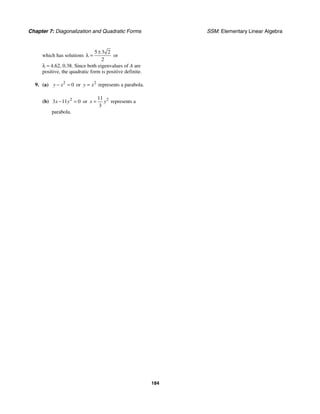
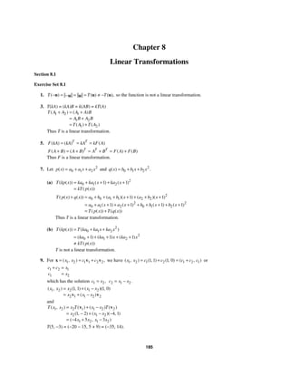
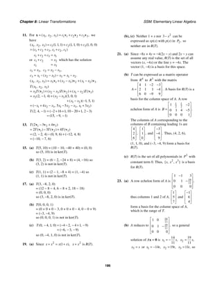
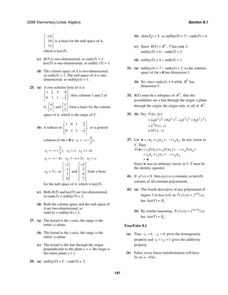
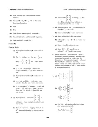
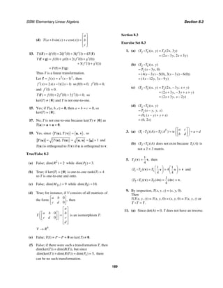
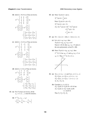
![SSM: Elementary Linear Algebra Section 8.4
191
(c) 1( , , ) ( , , )
T x y z kx ky kz
= and 2( , , ) ( cos sin , sin cos , )
T x y z x y x y z
θ θ θ θ
= − +
1 2
( )( , , ) ( ( cos sin ), ( sin sin ), )
T T x y z k x y k x y kz
θ θ θ θ
= − +
D
2 1
( )( , , ) ( cos sin , sin cos , )
T T x y z kx ky kx ky kz
θ θ θ θ
= − +
D
1 2 2
T T T T
=
D D
True/False 8.3
(a) True
(b) False; the linear operators in Exercise 21(b) are an example.
(c) False; a linear transformation need not have an inverse.
(d) True; for T to have an inverse, it must be one-to-one.
(e) False; 1
T−
does not exist.
(f) True; if 1
T is not one-to-one then there is some nonzero vector 1
v with 1 1
( ) ,
T =
v 0 then 2 1 1 2
( )( ) ( )
T T T
= =
v 0 0
D
and 2 1
ker( ) { }.
T T ≠ 0
D
Section 8.4
Exercise Set 8.4
1. (a) 1 2
1
( ) ( )
T T x
= = =
u v
2
2 3
( ) ( )
T T x x
= = =
u v
2 3
3 4
( ) ( )
T T x x
= = =
u v
Thus the matrix for T relative to B and B′ is
0 0 0
1 0 0
0 1 0
0 0 1
.
⎡ ⎤
⎢ ⎥
⎢ ⎥
⎢ ⎥
⎢ ⎥
⎣ ⎦
(b)
0
0
1
1
2
2
0
0 0 0
1 0 0
0 1 0
0 0 0
,
[ ] [ ]
B B B
c
c
T c
c
c
c
′
⎡ ⎤
⎡ ⎤
⎡ ⎤ ⎢ ⎥
⎢ ⎥
⎢ ⎥
= = ⎢ ⎥
⎢ ⎥
⎢ ⎥ ⎢ ⎥
⎢ ⎥
⎣ ⎦ ⎢ ⎥
⎢ ⎥
⎣ ⎦ ⎣ ⎦
x
2 3 0
0 1 2
1
2
0
[ ( )] [ ]
B B
c
T c x c x c x
c
c
′ ′
⎡ ⎤
⎢ ⎥
= + + = ⎢ ⎥
⎢ ⎥
⎢ ⎥
⎣ ⎦
x
3. (a) T(1) = 1
T(x) = x − 1 = −1 + x
2 2 2
1 1 2
( ) ( )
T x x x x
= − = − +
Thus the matrix for T relative to B is
1 1 1
0 1 2
0 0 1
.
−
⎡ ⎤
⎢ ⎥
−
⎢ ⎥
⎣ ⎦](https://image.slidesharecdn.com/elementary-linear-algebra-chapter1-220420115526/85/Elementary-linear-algebra-chapter-1-pdf-246-320.jpg)
![Chapter 8: Linear Transformations SSM: Elementary Linear Algebra
192
(b)
0
1
2
0 1 2
1 2
2
1 1 1
0 1 2
0 0 1
2
[ ] [ ]
B B
a
T a
a
a a a
a a
a
⎡ ⎤
−
⎡ ⎤
⎢ ⎥
⎢ ⎥
= −
⎢ ⎥
⎢ ⎥
⎣ ⎦ ⎣ ⎦
− +
⎡ ⎤
⎢ ⎥
= −
⎢ ⎥
⎣ ⎦
x
For 2
0 1 2 ,
a a x a x
= + +
x
2
0 1 2
2
0 1 2 1 2 2
1 1
2
( ) ( ) ( )
( ) ,
T a a x a x
a a a a a x a x
= + − + −
= − + + − +
x
so
0 1 2
1 2
2
2
[ ( )] .
B
a a a
T a a
a
− +
⎡ ⎤
⎢ ⎥
= −
⎢ ⎥
⎣ ⎦
x
5. (a) 1 1 2 2
7
1 8
1
0
1
3 2 3
0
( )
T T
⎡ ⎤
⎛ ⎞
⎡ ⎤ ⎢ ⎥
= = = − +
−
⎜ ⎟
⎢ ⎥ ⎢ ⎥
⎣ ⎦
⎝ ⎠
⎣ ⎦
u v v v
2 1 2 3
6
4
2
0
2
4 3
0
( )
T T
⎡ ⎤
⎛ ⎞
−
⎡ ⎤ ⎢ ⎥
= = = + +
⎜ ⎟
⎢ ⎥ ⎢ ⎥
⎣ ⎦
⎝ ⎠
⎣ ⎦
u v v v
1
2
8 4
3 3
0 0
1
,
[ ]B B
T ′
⎡ ⎤
⎢ ⎥
−
= ⎢ ⎥
⎢ ⎥
⎣ ⎦
7. (a) T(1) = 1
T(x) = 2x + 1 = 1 + 2x
2 2 2
2 1 1 4 4
( ) ( )
T x x x x
= + = + +
1 1 1
0 2 4
0 0 4
[ ]B
T
⎡ ⎤
⎢ ⎥
=
⎢ ⎥
⎣ ⎦
(b) The matrix for 2
2 3 4
x x
− + is
2
3
4
.
⎡ ⎤
⎢ ⎥
−
⎢ ⎥
⎣ ⎦
2 1 1 1 2 3
3 0 2 4 3 10
4 0 0 4 4 16
[ ]B
T
⎡ ⎤ ⎡ ⎤ ⎡ ⎤ ⎡ ⎤
⎢ ⎥ ⎢ ⎥ ⎢ ⎥ ⎢ ⎥
= =
− −
⎢ ⎥ ⎢ ⎥ ⎢ ⎥ ⎢ ⎥
⎣ ⎦ ⎣ ⎦ ⎣ ⎦ ⎣ ⎦
Thus 2 2
2 3 4 3 10 16
( ) .
T x x x x
− + = + +
(c) 2 2
2
2
2 3 4 2 3 2 1 4 2 1
2 6 3 16 16 4
3 10 16
( ) ( ) ( )
T x x x x
x x x
x x
− + = − + + +
= − − + + +
= + +
9. (a) Since A is the matrix for T relative to B,
[ ]
1 2 .
[ ( ) [ ( )]
B B
A T T
= v v That is,
1
1
2
[ ( )]B
T
⎡ ⎤
= ⎢ ⎥
−
⎣ ⎦
v and 2
3
5
[ ( )] .
B
T
⎡ ⎤
= ⎢ ⎥
⎣ ⎦
v
(b) Since 1
1
2
[ ( )] ,
B
T
⎡ ⎤
= ⎢ ⎥
−
⎣ ⎦
v
1 1 2
1 2 3
1 2
3 8 5
( ) .
T
−
⎡ ⎤ ⎡ ⎤ ⎡ ⎤
= − = − =
⎢ ⎥ ⎢ ⎥ ⎢ ⎥
−
⎣ ⎦ ⎣ ⎦ ⎣ ⎦
v v v
Similarly,
2 1 2
3 5 2
3 5
9 20 29
( ) .
T
− −
⎡ ⎤ ⎡ ⎤ ⎡ ⎤
= + = + =
⎢ ⎥ ⎢ ⎥ ⎢ ⎥
⎣ ⎦ ⎣ ⎦ ⎣ ⎦
v v v
(c) If 1
1 1 2 2 1 2
2
1 1
3 4
,
x
c c c c
x
−
⎡ ⎤ ⎡ ⎤ ⎡ ⎤
= + = +
⎢ ⎥ ⎢ ⎥ ⎢ ⎥
⎣ ⎦ ⎣ ⎦
⎣ ⎦
v v
then 1 1 2
2 1 2
3 4
x c c
x c c
= −
= +
. Solving for 1
c and 2
c
gives 1 1 2
4 1
7 7
,
c x x
= + 2 1 2
3 1
7 7
,
c x x
= − +
so
1
2
1 1 2 2
1 2 1 2
18 1
1 2
7 7
107 24
1 2
7 7
18 1
7 7 1
107 24
2
7 7
3 2
4 1 3 1
5 29
7 7 7 7
( ) ( )
x
T
x
c T c T
x x x x
x x
x x
x
x
⎛ ⎞
⎡ ⎤
⎜ ⎟
⎢ ⎥
⎣ ⎦
⎝ ⎠
= +
−
⎡ ⎤ ⎡ ⎤
⎛ ⎞ ⎛ ⎞
= +
+ − +
⎜ ⎟ ⎜ ⎟
⎢ ⎥ ⎢ ⎥
−
⎝ ⎠ ⎝ ⎠
⎣ ⎦ ⎣ ⎦
⎡ ⎤
+
⎢ ⎥
=
⎢ ⎥
− +
⎣ ⎦
⎡ ⎤ ⎡ ⎤
⎢ ⎥
= ⎢ ⎥
⎢ ⎥
− ⎣ ⎦
⎣ ⎦
v v
(d)
18 19
1
7 7 7
107 83
24
7 7 7
1 1
1 1
T
⎡ ⎤ ⎡ ⎤
⎛ ⎞
⎡ ⎤ ⎡ ⎤
⎢ ⎥ ⎢ ⎥
= =
⎜ ⎟
⎢ ⎥ ⎢ ⎥
⎢ ⎥ ⎢ ⎥
⎣ ⎦ − ⎣ ⎦ −
⎝ ⎠ ⎣ ⎦ ⎣ ⎦
11. (a) Since A is the matrix for T relative to B, the
columns of A are 1
[ ( )] ,
B
T v 2
[ ( )] ,
B
T v and
3
[ ( )] ,
B
T v respectively. That is,
1
1
2
6
[ ( )] ,
B
T
⎡ ⎤
⎢ ⎥
=
⎢ ⎥
⎣ ⎦
v 2
3
0
2
[ ( )] ,
B
T
⎡ ⎤
⎢ ⎥
=
⎢ ⎥
−
⎣ ⎦
v and
3
1
5
4
[ ( )] .
B
T
−
⎡ ⎤
⎢ ⎥
=
⎢ ⎥
⎣ ⎦
v](https://image.slidesharecdn.com/elementary-linear-algebra-chapter1-220420115526/85/Elementary-linear-algebra-chapter-1-pdf-247-320.jpg)
![SSM: Elementary Linear Algebra Section 8.4
193
(b) Since 1
1
2
6
[ ( )] ,
B
T
⎡ ⎤
⎢ ⎥
=
⎢ ⎥
⎣ ⎦
v
1
1 2 3
2 2 2
2
2 6
3 3 2 6 4 18 42 12
16 51 19
( )
.
T
x x x x x x
x x
= + +
= + − + + + + +
= + +
v
v v v
Similarly, 2 1 3
2 2
2
3 2
9 9 6 14 4
6 5 5
( )
,
T
x x x x
x x
= −
= + − − −
= − − +
v v v
and 3 1 2 3
2 2
2
2
5 4
3 3 5 15 10 12
28 8
7 40 15
( )
.
T
x x x x
x x
x x
= − + +
= − − − + + +
+ +
= + +
v v v v
(c) If 2
0 1 2
1 1 2 2 3 3
2 2
1 2
2
3
3 3 1 3 2
3 7 2
( ) ( )
( ),
a a x a x
c c c
c x x c x x
c x x
+ +
= + +
= + + − + +
+ + +
v v v
Then
0 2 3
1 1 2 3
2 1 2 3
3
3 3 7
3 2 2
a c c
a c c c
a c c c
= − +
= + +
= + +
.
Solving for 1,
c 2,
c and 3
c gives
1 0 1 2
1
2
3
( ),
c a a a
= − +
2 0 1 2
1
5 3 3
8
( ),
c a a a
= − + −
3 0 1 2
1
8
( ),
c a a a
= + − so
2
0 2
1 1 2 2 3 3
2
0 1 2
2
0 1 2
2
0 1 2
0 1 2
0 1 2
2
0 1 2
1
2 16 51 19
3
1
5 3 3 6 5 5
8
1
7 40 15
8
239 161 289
24
201 111 247
8
61 31 107
12
( , )
( ) ( ) ( )
( )( )
( )( )
( )( )
T a a x a x
c T c T c T
a a a x x
a a a x x
a a a x x
a a a
a a a
x
a a a
x
+ +
= + +
= − + + +
+ − + − − − +
+ + − + +
− +
=
− +
+
− +
+
v v v
(d) In 2
1 ,
x
+ 0 1,
a = 1 0,
a = 2 1.
a =
2
2
2
1
239 289 201 247 61 107
24 8 12
22 56 14
( )
T x
x x
x x
+
+ + +
= + +
= + +
13. (a) 2 1 2
1 2 6
( )( ) ( )
T T T x
= =
D
2
2 1 2 3 9
( )( ) ( )
T T x T x x
= − = −
D
Thus, 2 1
0 0
6 0
0 9
0 0
,
[ ] .
B B
T T ′
⎡ ⎤
⎢ ⎥
= ⎢ ⎥
−
⎢ ⎥
⎢ ⎥
⎣ ⎦
D
1 1 2
( )
T =
1 3
( )
T x x
= −
Thus 1
2 0
0 3
0 0
,
[ ] .
B B
T ′′
⎡ ⎤
⎢ ⎥
= −
⎢ ⎥
⎣ ⎦
2 1 3
( )
T x
=
2
2 3
( )
T x x
=
2 3
2 3
( )
T x x
=
Thus 2
0 0 0
3 0 0
0 3 0
0 0 3
,
[ ] .
B B
T ′ ′′
⎡ ⎤
⎢ ⎥
= ⎢ ⎥
⎢ ⎥
⎢ ⎥
⎣ ⎦
(b) 2 1 2 1
, , ,
[ ] [ ] [ ]
B B B B B B
T T T T
′ ′ ′′ ′′
=
D
(c)
0 0 0 0 0
2 0
3 0 0 6 0
0 3
0 3 0 0 9
0 0
0 0 3 0 0
⎡ ⎤ ⎡ ⎤
⎡ ⎤
⎢ ⎥ ⎢ ⎥
⎢ ⎥ =
−
⎢ ⎥ ⎢ ⎥
−
⎢ ⎥
⎢ ⎥ ⎢ ⎥
⎣ ⎦
⎢ ⎥ ⎢ ⎥
⎣ ⎦ ⎣ ⎦
15. If T is a contraction or dilation of V, then T maps
any basis 1 2
{ , , ..., }
n
B = v v v of V to
1 2
{ , , ..., }
n
k k k
v v v where k is a nonzero
constant. Thus the matrix for T relative to B is
0 0 0
0 0 0
0 0 0
0 0 0
.
k
k
k
k
⎡ ⎤
⎢ ⎥
⎢ ⎥
⎢ ⎥
⎢ ⎥
⎢ ⎥
⎣ ⎦
# # # #](https://image.slidesharecdn.com/elementary-linear-algebra-chapter1-220420115526/85/Elementary-linear-algebra-chapter-1-pdf-248-320.jpg)
![Chapter 8: Linear Transformations SSM: Elementary Linear Algebra
194
17. The matrix for T relative to B is the matrix
whose columns are the transforms of the basis
vectors in B in terms of the standard basis. Since
B is the standard basis for ,
n
R this matrix is the
standard matrix for T. Also, since B′ is the
standard basis for ,
m
R the resulting
transformation will give vector components
relative to the standard basis.
19. (a) 1 1 0
( ) ( )
D D
= =
f
2
( ) (sin ) cos
D D x x
= =
f
3
( ) (cos ) sin
D D x x
= = −
f
The matrix for D relative to this basis is
0 0 0
0 0 1
0 1 0
.
⎡ ⎤
⎢ ⎥
−
⎢ ⎥
⎣ ⎦
(b) 1 1 0
( ) ( )
D D
= =
f
2
( ) ( )
x x
D D e e
= =
f
2 2
3 2
( ) ( )
x x
D D e e
= =
f
The matrix for D relative to this basis is
0 0 0
0 1 0
0 0 2
.
⎡ ⎤
⎢ ⎥
⎢ ⎥
⎣ ⎦
(c) 2 2
1 2
( ) ( )
x x
D D e e
= =
f
2 2 2
2 2
( ) ( )
x x x
D D xe e xe
= = +
f
2 2 2 2 2
3 2 2
( ) ( )
x x x
D D x e xe x e
= = +
f
The matrix for D relative to this basis is
2 1 0
0 2 2
0 0 2
.
⎡ ⎤
⎢ ⎥
⎢ ⎥
⎣ ⎦
(d) 2 2 2 2
4 6 10
2 1 0 4
0 2 2 6
0 0 2 10
14
8
20
( )
x x x
D e xe x e
+ −
⎡ ⎤ ⎡ ⎤
⎢ ⎥ ⎢ ⎥
=
⎢ ⎥ ⎢ ⎥
−
⎣ ⎦ ⎣ ⎦
⎡ ⎤
⎢ ⎥
= −
⎢ ⎥
−
⎣ ⎦
Thus, 2 2 2 2
2 2 2 2
4 6 10
14 8 20
( )
.
x x x
x x x
D e xe x e
e xe x e
+ −
= − −
21. (a) 2 1 2 1
, , ,
[ ] [ ] [ ]
B B B B B B
T T T T
′ ′ ′′ ′′
=
D
(b) 3 2 1
3 2 1
,
, , ,
[ ]
[ ] [ ] [ ]
B B
B B B B B B
T T T
T T T
′
′ ′′′ ′′′ ′′ ′′
=
D D
True/False 8.4
(a) False; the conclusion would only be true if T:
V → V were a linear operator, i.e., if V = W.
(b) False; the conclusion would only be true if T:
V → V were a linear operator, i.e., if V = W.
(c) True; since the matrix for T is invertible, ker(T)
= {0}.
(d) False; the matrix of S T
D relative to B is
[ ] [ ] .
B B
S T
(e) True
Section 8.5
Exercise Set 8.5
1. 1
1
0
( )
T
⎡ ⎤
= ⎢ ⎥
⎣ ⎦
u and 2
2
1
( ) ,
T
−
⎡ ⎤
= ⎢ ⎥
−
⎣ ⎦
u so
1 2
0 1
[ ] .
B
T
−
⎡ ⎤
= ⎢ ⎥
−
⎣ ⎦
By inspection, 1 1 2
2
= +
v u u and
2 1 2
3 4 ,
= − +
v u u so the transition matrix from
B′ to B is
2 3
1 4
.
P
−
⎡ ⎤
= ⎢ ⎥
⎣ ⎦
Thus
3
4
1 11 11
1 2
11 11
.
B B
P P−
′
→
⎡ ⎤
⎢ ⎥
= =
−
⎢ ⎥
⎣ ⎦
3
4
11 11
1 2
11 11
3 56
11 11
3
2
11 11
1 2 2 3
0 1 1 4
[ ] [ ]
B B B B B B
T P T P
′ ′ ′
→ →
=
⎡ ⎤ − −
⎡ ⎤ ⎡ ⎤
⎢ ⎥
= ⎢ ⎥ ⎢ ⎥
−
− ⎣ ⎦ ⎣ ⎦
⎢ ⎥
⎣ ⎦
⎡ ⎤
− −
⎢ ⎥
=
−
⎢ ⎥
⎣ ⎦](https://image.slidesharecdn.com/elementary-linear-algebra-chapter1-220420115526/85/Elementary-linear-algebra-chapter-1-pdf-249-320.jpg)
![SSM: Elementary Linear Algebra Section 8.5
195
3. Since B is the standard basis for 2
,
R
1 1
2 2
1 1
2 2
45 45
45 45
cos sin
[ ] .
sin cos
B
T
⎡ ⎤
−
° − °
⎡ ⎤ ⎢ ⎥
= =
⎢ ⎥
° ° ⎢ ⎥
⎣ ⎦
⎣ ⎦
The
matrices for B B
P ′
→ and B B
P ′↔ are the same as
in Exercise 1, so
1 1
3
4
2 2
11 11
1 1
1 2
11 11 2 2
13 25
11 2 11 2
5 9
11 2 11 2
2 3
1 4
[ ] [ ]
.
B B B B B B
T P T P
′ ′ ′
→ →
=
⎡ ⎤
−
⎡ ⎤ −
⎡ ⎤
⎢ ⎥
⎢ ⎥
= ⎢ ⎥
⎢ ⎥
− ⎣ ⎦
⎢ ⎥
⎣ ⎦ ⎣ ⎦
⎡ ⎤
−
⎢ ⎥
=
⎢ ⎥
⎣ ⎦
5. 1
1
0
0
( ) ,
T
⎡ ⎤
⎢ ⎥
=
⎢ ⎥
⎣ ⎦
u 2
0
1
0
( )
T
⎡ ⎤
⎢ ⎥
=
⎢ ⎥
⎣ ⎦
u and 3
0
0
0
( ) ,
T
⎡ ⎤
⎢ ⎥
=
⎢ ⎥
⎣ ⎦
u so
1 0 0
0 1 0
0 0 0
[ ] .
B
T
⎡ ⎤
⎢ ⎥
=
⎢ ⎥
⎣ ⎦
By inspection, 1 1,
=
v u 2 1 2,
= +
v u u and
3 1 2 3,
= + +
v u u u so the transition matrix from
B′ to B is
1 1 1
0 1 1
0 0 1
.
P
⎡ ⎤
⎢ ⎥
=
⎢ ⎥
⎣ ⎦
Thus 1
1 1 0
0 1 1
0 0 1
B B
P P−
′
→
−
⎡ ⎤
⎢ ⎥
= = −
⎢ ⎥
⎣ ⎦
and
1 1 0 1 0 0 1 1 1
0 1 1 0 1 0 0 1 1
0 0 1 0 0 0 0 0 1
1 0 0
0 1 1
0 0 0
[ ] [ ]
.
B B B B B B
T P T P
′ ′ ′
→ →
=
−
⎡ ⎤ ⎡ ⎤ ⎡ ⎤
⎢ ⎥ ⎢ ⎥ ⎢ ⎥
= −
⎢ ⎥ ⎢ ⎥ ⎢ ⎥
⎣ ⎦ ⎣ ⎦ ⎣ ⎦
⎡ ⎤
⎢ ⎥
=
⎢ ⎥
⎣ ⎦
7. 1 1 2
2 1
6 3 1 9 3
3 2
( ) ( ) ,
T x x
= + + = + = +
p p p and
2 1 2
2 4
10 2 1 12 2
9 3
( ) ( ) ,
T x x
= + + = + = − +
p p p
so
2 2
3 9
1 4
2 3
[ ] .
B
T
⎡ ⎤
−
⎢ ⎥
=
⎢ ⎥
⎣ ⎦
1 1 2
2 1
9 3
= − +
q p p and 2 1 2
7
9 6
,
1
= −
q p p so the
transition matrix from B′ to B is
7
2
9 9
1 1
3 6
.
P
⎡ ⎤
−
⎢ ⎥
=
−
⎢ ⎥
⎣ ⎦
Thus
3 7
1 4 2
3
2
1
B B
P P−
′
→
⎡ ⎤
⎢ ⎥
= =
⎢ ⎥
⎣ ⎦
and
7
3 7 2 2 2
3 9 9 9
4 2
3 1 4 1 1
2 3 3 6
2
1
1 1
0 1
[ ] [ ]
.
B B B B B B
T P T P
′ ′ ′
→ →
=
⎡ ⎤
⎡ ⎤ ⎡ ⎤
− −
⎢ ⎥
⎢ ⎥ ⎢ ⎥
=
−
⎢ ⎥
⎢ ⎥ ⎢ ⎥
⎣ ⎦ ⎣ ⎦ ⎣ ⎦
⎡ ⎤
= ⎢ ⎥
⎣ ⎦
11. (a) The matrix for T relative to the standard
basis B is
1 1
2 4
[ ] .
B
T
−
⎡ ⎤
= ⎢ ⎥
⎣ ⎦
The eigenvalues
of [ ]B
T are λ = 2 and λ = 3 with
corresponding eigenvectors
1
1
⎡ ⎤
⎢ ⎥
−
⎣ ⎦
and
1
2
.
⎡ ⎤
⎢ ⎥
−
⎣ ⎦
Then for
1 1
1 2
,
P
⎡ ⎤
= ⎢ ⎥
− −
⎣ ⎦
we have
1 2 1
1 1
P− ⎡ ⎤
= ⎢ ⎥
− −
⎣ ⎦
and 1 2 0
0 3
[ ] .
B
P T P
− ⎡ ⎤
= ⎢ ⎥
⎣ ⎦
Since P represents the transition matrix from
the basis B′ to the standard basis B, then
1 1
1 2
,
B
⎧ ⎫
⎡ ⎤ ⎡ ⎤
′ = ⎨ ⎬
⎢ ⎥ ⎢ ⎥
− −
⎣ ⎦ ⎣ ⎦
⎩ ⎭
is a basis for which
[ ]B
T ′ is diagonal.
(b) The matrix for T relative to the standard
basis B is
4 1
3 1
[ ] .
B
T
−
⎡ ⎤
= ⎢ ⎥
−
⎣ ⎦
The eigenvalues of [ ]B
T are
5 21
2
+
λ =
and
5 21
2
−
λ = with corresponding
eigenvectors
3 21
6
1
− −
⎡ ⎤
⎢ ⎥
⎢ ⎥
⎣ ⎦
and
3 21
6
1
.
− +
⎡ ⎤
⎢ ⎥
⎢ ⎥
⎣ ⎦
Then for
3 21 3 21
6 6
1 1
,
P
− − − +
⎡ ⎤
= ⎢ ⎥
⎢ ⎥
⎣ ⎦
we have
3 21
3
1 21 2 21
3 21
3
21 2 21
P
− +
−
+
⎡ ⎤
−
⎢ ⎥
= ⎢ ⎥
⎢ ⎥
⎣ ⎦
and](https://image.slidesharecdn.com/elementary-linear-algebra-chapter1-220420115526/85/Elementary-linear-algebra-chapter-1-pdf-250-320.jpg)
![Chapter 8: Linear Transformations SSM: Elementary Linear Algebra
196
5 21
1 2
5 21
2
0
0
[ ] .
B
P I P
+
−
−
⎡ ⎤
⎢ ⎥
=
⎢ ⎥
⎣ ⎦
Since P
represents the transition matrix from the
basis B′ to the standard basis B, then
3 21 3 21
6 6
1 1
,
B
− − − +
⎧ ⎫
⎡ ⎤ ⎡ ⎤
⎪ ⎪
′ = ⎢ ⎥ ⎢ ⎥
⎨ ⎬
⎢ ⎥ ⎢ ⎥
⎪ ⎪
⎣ ⎦ ⎣ ⎦
⎩ ⎭
is a basis for
which [ ]B
T ′ is diagonal.
13. (a) 2
1 5
( )
T x
= +
T(x) = 6 − x
2 2
2 8 2
( )
T x x x
= − −
Thus the matrix for T relative to the standard
basis B is
5 6 2
0 1 8
1 0 2
[ ] .
B
T
⎡ ⎤
⎢ ⎥
= − −
⎢ ⎥
−
⎣ ⎦
The
characteristic equation for [ ]B
T is
3 2 2
2 15 36 4 3 0
( )( ) ,
λ − λ − λ + = λ + λ − = so
the eigenvalues of T are λ = −4 and λ = 3.
(b) A basis for the eigenspace corresponding to
λ = −4 is 8
3
2
1
,
−
⎡ ⎤
⎢ ⎥
⎢ ⎥
⎢ ⎥
⎣ ⎦
so the polynomial
2
8
2
3
x x
− + + is a basis in 2
.
P A basis for
the eigenspace corresponding to λ = 3 is
5
2
1
,
⎡ ⎤
⎢ ⎥
−
⎢ ⎥
⎣ ⎦
so the polynomial so the polynomial
2
5 2x x
− + is a basis in 2
.
P
15. If v is an eigenvector of T corresponding to λ,
then v is a nonzero vector which satisfies the
equation T(v) = λv or (λI − T)(v) = 0. Thus v is
in the kernel of λI − T.
17. Since [ ] [ ]
B B
C D
=
x x for all x in V, then we can
let i
=
x v for each of the basis vectors
1, ..., n
v v of V. Since [ ]
i B i
=
v e for each i
where 1
{ , ..., }
n
e e is the standard basis for ,
n
R
this yields i i
C D
=
e e for i = 1, 2, ..., n. But i
Ce
and i
De are the ith columns of C and D,
respectively. Since corresponding columns of C
and D are all equal, C = D.
True/False 8.5
(a) False; every matrix is similar to itself since
1
.
A I AI
−
=
(b) True; if 1
A P BP
−
= and 1
,
B Q CQ
−
= then
1 1 1
( ) ( ) ( ).
A P Q CQ P QP C QP
− − −
= =
(c) True; invertibility is a similarity invariant.
(d) True; if 1
,
A P BP
−
= then
1 1 1 1 1
( ) .
A P BP P B P
− − − − −
= =
(e) True
(f) False; for example, let T be the zero operator.
(g) True
(h) False; if B and B′ are different, let [ ]B
T be
given by the matrix .
B B
P ′
→ Then
,
[ ] [ ] .
B B B B B B B B B n
T P T P P I
′ ′ ′ ′
→ → →
= = =
Chapter 8 Supplementary Exercises
1. No; 1 2 1 2
1 2
1 2
( ) ( )
) ( )
( ) ( ),
T A B
A B A B
T T
+ = + +
≠ ( + + +
= +
x x x x
x x
x x
and if c ≠ 1, then
( ) ( ) ( ).
T c cA B c A B cT
= + ≠ + =
x x x x
3. ( ) ( )
T k k k k k kT
= = ≠
v v v v v v if k ≠ 1.
5. (a) The matrix for T relative to the standard
basis is
1 0 1 1
2 1 3 1
1 0 0 1
.
A
⎡ ⎤
⎢ ⎥
=
⎢ ⎥
⎣ ⎦
A basis for the
range of T is a basis for the column space of
A. A reduces to
1 0 0 1
0 1 0 1
0 0 1 0
.
⎡ ⎤
⎢ ⎥
−
⎢ ⎥
⎣ ⎦
Since row operations don’t change the
dependency relations among columns, the
reduced form of A indicates that 3
( )
T e and
any two of 1
( ),
T e 2
( ),
T e 4
( )
T e form a
basis for the range.
The reduced form of A shows that the
general solution of Ax = 0 is x = −s, 2 ,
x s
=](https://image.slidesharecdn.com/elementary-linear-algebra-chapter1-220420115526/85/Elementary-linear-algebra-chapter-1-pdf-251-320.jpg)
![SSM: Elementary Linear Algebra Chapter 8 Supplementary Exercises
197
3 0,
x = 4
x s
= so a basis for the null space
of A, which is the kernel of T is
1
1
0
1
.
−
⎡ ⎤
⎢ ⎥
⎢ ⎥
⎢ ⎥
⎢ ⎥
⎣ ⎦
(b) Since R(T) is three-dimensional and ker(T)
is one-dimensional, rank(T) = 3 and
nullity(T) = 1.
7. (a) The matrix for T relative to B is
1 1 2 2
1 1 4 6
1 2 5 6
3 2 3 2
[ ] .
B
T
−
⎡ ⎤
⎢ ⎥
− −
= ⎢ ⎥
−
⎢ ⎥
−
⎢ ⎥
⎣ ⎦
[ ]B
T reduces to
1 0 1 2
0 1 3 4
0 0 0 0
0 0 0 0
−
⎡ ⎤
⎢ ⎥
−
⎢ ⎥
⎢ ⎥
⎢ ⎥
⎣ ⎦
which
has rank 2 and nullity 2. Thus, rank(T) = 2
and nullity(T) = 2.
(b) Since rank(T) dim(V), T is not one-to-one.
9. (a) Since 1
,
A P BP
−
= then
1 1
1 1 1
1 1 1
( ) ( )
(( ) ) ( )
(( ) ) ( ) .
T T T T T
T T T
T T T
A P BP P B P
P B P
P B P
− −
− − −
− − −
= =
=
=
Thus, T
A and T
B are similar.
(b) 1 1 1 1 1
( )
A P BP P B P
− − − − −
= =
Thus 1
A−
and 1
B−
are similar.
11. For ,
a b
X
c d
⎡ ⎤
= ⎢ ⎥
⎣ ⎦
0 0
2
( )
.
a c b d b b
T X
d d
a b c b d
d d
+ +
⎡ ⎤ ⎡ ⎤
= +
⎢ ⎥ ⎢ ⎥
⎣ ⎦ ⎣ ⎦
+ + +
⎡ ⎤
= ⎢ ⎥
⎣ ⎦
T(X) = 0 gives the equations
0
2 0
0.
a b c
b d
d
+ + =
+ =
=
Thus c = −a and X is in ker(T) if it has the form
0
0
,
k
k
⎡ ⎤
⎢ ⎥
−
⎣ ⎦
so
1 0
1 0
ker( )
T k
⎧ ⎫
⎡ ⎤
= ⎨ ⎬
⎢ ⎥
−
⎣ ⎦
⎩ ⎭
which is
one-dimensional. Hence, nullity(T) = 1 and
22
rank nullity 3
( ) dim( ) ( ) .
T M T
= − =
13. The standard basis for 22
M is 1
1 0
0 0
,
⎡ ⎤
= ⎢ ⎥
⎣ ⎦
u
2
0 1
0 0
,
⎡ ⎤
= ⎢ ⎥
⎣ ⎦
u 3
0 0
1 0
,
⎡ ⎤
= ⎢ ⎥
⎣ ⎦
u 4
0 0
0 1
.
⎡ ⎤
= ⎢ ⎥
⎣ ⎦
u Since
1 1
( ) ,
L =
u u 2 3
( ) ,
L =
u u 3 2
( ) ,
L =
u u and
4 4
( ) ,
L =
u u the matrix of L relative to the
standard basis is
1 0 0 0
0 0 1 0
0 1 0 0
0 0 0 1
.
⎡ ⎤
⎢ ⎥
⎢ ⎥
⎢ ⎥
⎢ ⎥
⎣ ⎦
15. The transition matrix from B′ to B is
1 1 1
0 1 1
0 0 1
,
P
⎡ ⎤
⎢ ⎥
=
⎢ ⎥
⎣ ⎦
thus
1
4 0 9
1 0 2
0 1 1
[ ] [ ] .
B B
T P T P
−
′
−
⎡ ⎤
⎢ ⎥
= = −
⎢ ⎥
⎣ ⎦
17.
1 1
0 0
0 1
,
T
⎛ ⎞
⎡ ⎤ ⎡ ⎤
⎜ ⎟
⎢ ⎥ ⎢ ⎥
=
⎜ ⎟
⎢ ⎥ ⎢ ⎥
⎜ ⎟
⎣ ⎦ ⎣ ⎦
⎝ ⎠
0 1
1 1
0 0
,
T
⎛ ⎞ −
⎡ ⎤ ⎡ ⎤
⎜ ⎟
⎢ ⎥ ⎢ ⎥
=
⎜ ⎟
⎢ ⎥ ⎢ ⎥
⎜ ⎟
⎣ ⎦ ⎣ ⎦
⎝ ⎠
and
0 1
0 0
1 1
,
T
⎛ ⎞
⎡ ⎤ ⎡ ⎤
⎜ ⎟
⎢ ⎥ ⎢ ⎥
=
⎜ ⎟
⎢ ⎥ ⎢ ⎥
⎜ ⎟ −
⎣ ⎦ ⎣ ⎦
⎝ ⎠
thus
1 1 1
0 1 0
1 0 1
[ } .
B
T
−
⎡ ⎤
⎢ ⎥
=
⎢ ⎥
−
⎣ ⎦
Note that this can also be read directly from
[ ( )] .
B
T x
19. (a) ( ) ( ( ) ( )) ( ) ( )
D f x g x f x g x
′′ ′′ ′′
+ = + = +
f g
and ( ) ( ( )) ( ).
D k kf x kf x
′′ ′′
= =
f
(b) If f is in ker(D), then f has the form
0 1
( ) ,
f x a a x
= = +
f so a basis for ker(D) is
f(x) = 1, g(x) = x.
(c) D(f) = f if and only if ( ) x x
f x ae be−
= = +
f
for arbitrary constants a and b. Thus,
( ) x
f x e
= and ( ) x
g x e−
= form a basis for
this subspace.](https://image.slidesharecdn.com/elementary-linear-algebra-chapter1-220420115526/85/Elementary-linear-algebra-chapter-1-pdf-252-320.jpg)
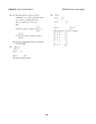
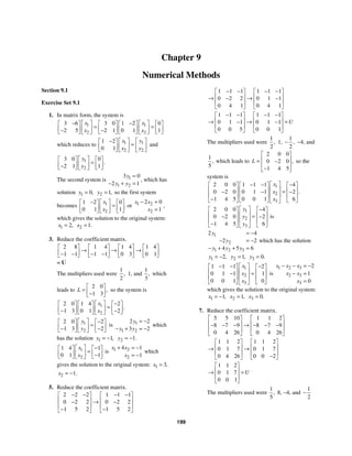
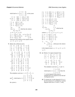
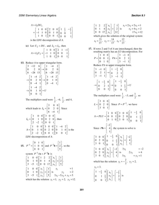
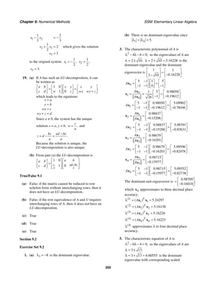
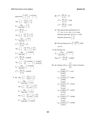
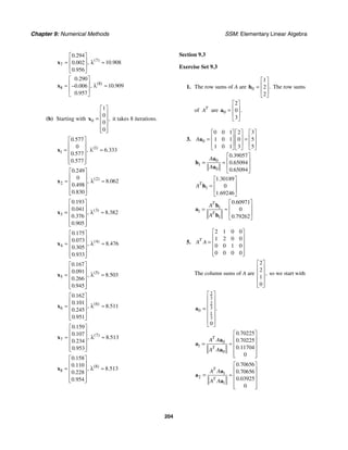
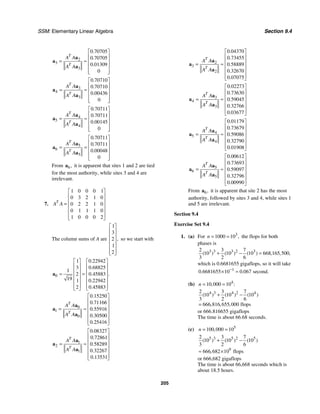
![Chapter 9: Numerical Methods SSM: Elementary Linear Algebra
206
3. 4
10 000 10
,
n = =
(a) 3 12 9
2 2
10 666 67 10
3 3
( ) .
n ≈ ≈ ×
666.67 gigaflops are required, which will
take
666 67
9 52 seconds.
70
.
.
≈
(b) 2 8 9
10 0 1 10
.
n ≈ = ×
0.1 gigaflop is required, which will take
about 0.0014 second.
(c) This is the same as part (a); about
9.52 seconds.
(d) 3 12 9
2 2 10 2000 10
n ≈ × = ×
2000 gigaflops are required, which will take
about 28.57 seconds.
5. (a) 5
100 000 10
,
n = =
3 15
15
5 9
2 2
10
3 3
0 667 10
6 67 10 10
.
.
n ≈ ×
≈ ×
= × ×
Thus, the forward phase would require
about 5
6 67 10 seconds.
. ×
2 10 9
10 10 10
n = = ×
The backward phase would require about
10 seconds.
(b) 4
10 000 10
,
n = =
3 12
12
2 9
2 2
10
3 3
0 667 10
6 67 10 10
.
.
n ≈ ×
≈ ×
≈ × ×
About 667 gigaflops are required, so the
computer would have to execute
2(667) = 1334 gigaflops per second.
7. Multiplying each of the 2
n entries of A by c
requires 2
flops.
n
9. Let [ ] .
ij
C c AB
= = Computing ij
c requires first
multiplying each of the n entries ik
a by the
corresponding entry ,
kj
b which requires n flops.
Then the n terms ik kj
a b must be summed, which
requires n − 1 flops. Thus, each of the 2
n entries
in AB requires 2n − 1 flops, for a total of
2 3 2
2 1 2 flops.
( )
n n n n
− = −
Note that adding two numbers requires 1 flop,
adding three numbers requires 2 flops, and in
general, n − 1 flops are required to add
n numbers.
Section 9.5
Exercise Set 9.5
1. The characteristic polynomial of
1 1 2 0
1 2 0
2 2 4 0
0 0 0 0
[ ]
T
A A
⎡ ⎤ ⎡ ⎤
⎢ ⎥ ⎢ ⎥
= =
⎢ ⎥ ⎢ ⎥
⎣ ⎦ ⎣ ⎦
is 2
5
( );
λ λ −
thus the eigenvalues of T
A A are 1 5
λ = and
2 0,
λ = and 1 5
σ = and 2 0
σ = are singular
values of A.
3. The eigenvalues of
1 2 1 2 5 0
2 1 2 1 0 5
T
A A
−
⎡ ⎤ ⎡ ⎤ ⎡ ⎤
= =
⎢ ⎥ ⎢ ⎥ ⎢ ⎥
−
⎣ ⎦ ⎣ ⎦ ⎣ ⎦
are 1 5
λ =
and 2 5
λ = (i.e., λ = 5 is an eigenvalue of
multiplicity 2); thus the singular value of A is
1 5.
σ =
5. The only eigenvalue of
1 1 1 1 2 0
1 1 1 1 0 2
T
A A
−
⎡ ⎤ ⎡ ⎤ ⎡ ⎤
= =
⎢ ⎥ ⎢ ⎥ ⎢ ⎥
−
⎣ ⎦ ⎣ ⎦ ⎣ ⎦
is λ = 2
(multiplicity 2), and the vectors 1
1
0
⎡ ⎤
= ⎢ ⎥
⎣ ⎦
v and
2
0
1
⎡ ⎤
= ⎢ ⎥
⎣ ⎦
v form an orthonormal basis for the
eigenspace (which is all of 2
).
R The singular
values of A are 1 2
σ = and 2 2.
σ = We have
1
2
1 1 1
1
2
1 1 1 1 1
1 1 0
2
,
A
σ
⎡ ⎤
−
⎡ ⎤ ⎡ ⎤ ⎢ ⎥
= = =
⎢ ⎥ ⎢ ⎥ ⎢ ⎥
⎣ ⎦ ⎣ ⎦
⎣ ⎦
u v and
1
2
2 2 1
2
2
1 1 1 1 0
1 1 1
2
.
A
σ
⎡ ⎤
−
−
⎡ ⎤ ⎡ ⎤ ⎢ ⎥
= = =
⎢ ⎥ ⎢ ⎥ ⎢ ⎥
⎣ ⎦ ⎣ ⎦
⎣ ⎦
u v This
results in the following singular value
decomposition of A:
1 1
2 2
1 1
2 2
2 0 1 0
0 1
0 2
T
A U V
⎡ ⎤
− ⎡ ⎤ ⎡ ⎤
⎢ ⎥
= Σ = ⎢ ⎥ ⎢ ⎥
⎢ ⎥ ⎣ ⎦
⎣ ⎦
⎣ ⎦](https://image.slidesharecdn.com/elementary-linear-algebra-chapter1-220420115526/85/Elementary-linear-algebra-chapter-1-pdf-261-320.jpg)
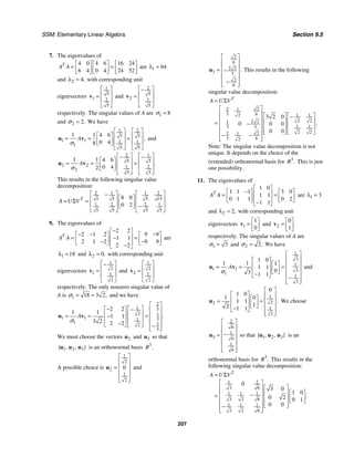
![Chapter 9: Numerical Methods SSM: Elementary Linear Algebra
208
True/False 9.5
(a) False; if A is an m × n matrix, then T
A is an
n × m matrix, and T
A A is an n × n matrix.
(b) True
(c) False; T
A A may have eigenvalues that are 0.
(d) False; A would have to be symmetric to be
orthogonally diagonalizable.
(e) True; since T
A A is a symmetric n × n matrix.
(f) False; the eigenvalues of T
A A are the squares of
the singular values of A.
(g) True
Section 9.6
Exercise Set 9.6
1. From Exercise 9 in Section 9.5, A has the
singular value decomposition
2
2 1
3 6 1 1
2
2 2
2 2
1
1 1
3 3
2 2
2
2 1
3 6
2
3 2 0
0 0 0
0 0
A
⎡ ⎤
⎢ ⎥ ⎡ ⎤
⎡ ⎤ −
⎢ ⎥ ⎢ ⎥
⎢ ⎥
= −
⎢ ⎥ ⎢ ⎥
⎢ ⎥
⎢ ⎥ ⎢ ⎥ ⎢ ⎥
⎣ ⎦ ⎣ ⎦
− −
⎢ ⎥
⎣ ⎦
where the lines show the relevant blocks. Thus
the reduced singular value decomposition of A is
[ ]
2
3
1 1
1
1 1 1 3 2 2
2
3
3 2 .
T
A U V
⎡ ⎤
⎢ ⎥
⎡ ⎤
−
= Σ = ⎢ ⎥
⎣ ⎦
⎢ ⎥
−
⎢ ⎥
⎣ ⎦
3. From Exercise 11 in Section 9.5, A has the
singular value decomposition
1 2
3 6
1 1 1
3 2 6
1 1 1
3 2 6
0
3 0
1 0
0 2 0 1
0 0
A
⎡ ⎤
⎡ ⎤
⎢ ⎥
⎡ ⎤
⎢ ⎥
⎢ ⎥
−
= ⎢ ⎥
⎢ ⎥
⎢ ⎥ ⎣ ⎦
⎢ ⎥
⎢ ⎥ ⎣ ⎦
−
⎢ ⎥
⎣ ⎦
where the lines indicate the relevant blocks.
Thus the reduced singular value decomposition
of A is
1
3
1 1
1 1 1 3 2
1 1
3 2
0
3 0 1 0
0 1
0 2
.
T
A U V
⎡ ⎤
⎢ ⎥
⎡ ⎤ ⎡ ⎤
⎢ ⎥
= Σ = ⎢ ⎥ ⎢ ⎥
⎢ ⎥ ⎣ ⎦
⎣ ⎦
⎢ ⎥
−
⎢ ⎥
⎣ ⎦
5. The reduced singular value expansion of A is
2
3
1 1
1
3 2 2
2
3
3 2 .
⎡ ⎤
⎢ ⎥
⎡ ⎤
−
⎢ ⎥
⎣ ⎦
⎢ ⎥
−
⎢ ⎥
⎣ ⎦
7. The reduced singular value decomposition of A
is
1
3
1
1
2
3
1
1
2
3
0
3 1 0 2 0 1
[ ] [ ].
⎡ ⎤ ⎡ ⎤
⎢ ⎥ ⎢ ⎥
⎢ ⎥ + ⎢ ⎥
⎢ ⎥ ⎢ ⎥
⎢ ⎥
− ⎢ ⎥
⎣ ⎦
⎢ ⎥
⎣ ⎦
9. A rank 100 approximation of A requires storage
space for 100(200 + 500 + 1) = 70,100 numbers,
while A has 200(500) = 100,000 has entries.
True/False 9.6
(a) True
(b) True
(c) False; 1
V has size n × k so that 1
T
V has size
k × n.
Chapter 9 Supplementary Exercises
1. Reduce A to upper triangular form.
6 2 3 1 3 1
6 0 6 0 0 2
U
− − −
⎡ ⎤ ⎡ ⎤ ⎡ ⎤
→ → =
⎢ ⎥ ⎢ ⎥ ⎢ ⎥
⎣ ⎦ ⎣ ⎦ ⎣ ⎦
The multipliers used were
1
2
and 2, so
2 0
2 1
L
⎡ ⎤
= ⎢ ⎥
−
⎣ ⎦
and
2 0 3 1
2 1 0 2
.
A
−
⎡ ⎤ ⎡ ⎤
= ⎢ ⎥ ⎢ ⎥
−
⎣ ⎦ ⎣ ⎦
3. Reduce A to upper triangular form.
2 4 6 1 2 3 1 2 3
1 4 7 1 4 7 0 2 4
1 3 7 1 3 7 1 3 7
⎡ ⎤ ⎡ ⎤ ⎡ ⎤
⎢ ⎥ ⎢ ⎥ ⎢ ⎥
→ →
⎢ ⎥ ⎢ ⎥ ⎢ ⎥
⎣ ⎦ ⎣ ⎦ ⎣ ⎦
1 2 3 1 2 3 1 2 3
0 2 4 0 1 2 0 1 2
0 1 4 0 1 4 0 0 2
⎡ ⎤ ⎡ ⎤ ⎡ ⎤
⎢ ⎥ ⎢ ⎥ ⎢ ⎥
→ → →
⎢ ⎥ ⎢ ⎥ ⎢ ⎥
⎣ ⎦ ⎣ ⎦ ⎣ ⎦
1 2 3
0 1 2
0 0 1
U
⎡ ⎤
⎢ ⎥
→ =
⎢ ⎥
⎣ ⎦
The multipliers used were
1
2
, −1, −1,
1
2
, −1,](https://image.slidesharecdn.com/elementary-linear-algebra-chapter1-220420115526/85/Elementary-linear-algebra-chapter-1-pdf-263-320.jpg)
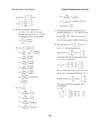
![Chapter 9: Numerical Methods SSM: Elementary Linear Algebra
210
11. A has rank 2, thus 1 1 2
[ ]
U = u u and
1
1
2
T
T
T
V
⎡ ⎤
= ⎢ ⎥
⎢ ⎥
⎣ ⎦
v
v
and the reduced singular value
decomposition of A is
1 1 1
1 1
2 2
2 1 2
1 1
3 3 3
2 2
1 1 2 2 1
2 2 3 3 3
1 1
2 2
24 0
0 12
T
A U V
= Σ
⎡ ⎤
⎢ ⎥
⎡ ⎤
−
−
⎢ ⎥ ⎡ ⎤ ⎢ ⎥
= ⎢ ⎥ ⎢ ⎥
− −
⎣ ⎦ ⎢ ⎥
⎢ ⎥ ⎣ ⎦
⎢ ⎥
⎢ ⎥
⎣ ⎦](https://image.slidesharecdn.com/elementary-linear-algebra-chapter1-220420115526/85/Elementary-linear-algebra-chapter-1-pdf-265-320.jpg)