Ac circuits

www.ekeeda.com Contact : 9029006464 Email : care@ekeeda.com
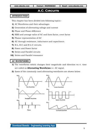
1
P
INTRODUCTION
This chapter has been divided into following topics:-
1) AC Waveforms and their advantages
2) Generation of alternating voltage and current
3) Phase and Phase difference
4) RMS and average value of AC and form factor, crest factor
5) Phasor representation of AC
6) AC through resistance, inductance and capacitance.
7) R-L, R-C and R-L-C circuits.
8) Power and Power factor
9) Series and Parallel circuits
10) Series and Parallel resonance
AC WAVEFORMS
1) The waveforms which changes their magnitude and direction w.r.t. time
are called as Alternating Waveforms i.e. AC signal.
2) Some of the commonly used alternating waveforms are shown below:
A.C. Circuits

2
Advantages of AC Signal
Out of all these types of alternating waveforms, sinusoidal waveform is
considered as basic AC signal. The advantages of sinusoidal signal are
1) Sinusoidal waveforms can be easily generated.
2) Any other AC signal can be expressed as sum of series of sine components.
3) Analysis of linear circuit with sinusoidal excitation is easy.
4) Sum and difference of two sine waves is a sine wave.
5) The integration and derivative of a sinusoidal function is again a
sinusoidal function.
Generation of AC
 Construction:-
1) It consists of a single turn rectangular coil (ABCD) made up of some
conducting material like copper or aluminium.
2) The coil is so placed that it can be rotated about its own axis at a
constant speed in a uniform magnetic field provided by the North and
South poles of the magnet.
3) The coil is known as armature of the alternator. The ends of the
alternator coil are connected to rings called slip rings which rotate with
armature.
4) Two carbon brushes pressed against the slip rings collect the current
induced in the coil and carry it to external resistor R.

3
 Working:
 Case i ( o
θ = 0 ):
1. This is the initial position of the coil. The plane of the coil being
perpendicular to the magnetic field, the conductors (A and B) of the
coil move parallel to the magnetic field.
2. Since, there is no flux cutting, no emf is generated in the conductors
and therefore, no current flows through the external circuit.
 Case ii ( o
θ = 90 ):
1. As the coil rotates from ( o
θ = 0 ) to ( o
θ = 90 ), more lines of force are
cut by the conductors.
2. In this case both the conductors of the coil move at right angles to
the magnetic field and cut through a maximum number of lines of
force, so a maximum emf is induced in them.
 Case iii ( o
θ=180 ):
1. When the coil rotates from ( o
θ = 0 ) to ( o
θ=180 ) (i.e. first half
revolution), again the plane of the coil becomes perpendicular to the
magnetic field. Thus, the emf again reaches to zero.
2. During the interval 0o to 180o the output voltage remains positive.
 Case iv ( o
θ=270 ):
1. As the coil rotates from ( o
θ=180 ) to ( o
θ = 270 ), more lines of force are
cut by the conductors and emf starts building up in negative
direction.
2. At o
θ = 270 the emf becomes maximum negative and thereafter it
starts decreasing.

4
EQUATION OF SINE WAVE
1) Consider a rectangular coil ABCD placed in a magnetic field generated by
permanent magnet. The coil with constant angular velocity in filed. These
causes generation of alternating emf in the coil.
2) Let, B = Flux Density (Wb/m2)
l = Active length of each Conductor (m)
r = Radius of circular path traced by conductors (m)
 = Angular velocity of coil (rad/s)
v = Linear velocity of each conductor (m/s)
3) Consider an instant where coil has rotated through an angle ‘θ ’ from
initial position. (i.e. o
θ = 0 ). It requires time ‘t’ to rotate through θ . So θ in
radians can be expressed as
θ = t rad
4) The position of coil is shown in fig. The instantaneous velocity of any
conductor can be resolved into two components as shown in figure:
5) The components of velocity v are:
a) Parallel to the direction of magnetic field = v cos θ
b) Perpendicular to direction of magnetic field = v sin θ
6) EMF induced due to parallel component is zero, since there is no cutting of
flux. Thus, the perpendicular component is responsible for emf generation.
7) According to Faraday’s law of electromagnetic induction, the expression for
the generated emf in each conductor is
vsinθe Bl (Volts)

5
8) The active length ‘l ’ means the length of conductor which is under
influence of magnetic field. Now,
Em = Bl v = Maximum induced emf in conductor
This is possible at o
θ = 90
9) Hence instantaneous value of induced emf is given by,
me = E sinθ
But θ= ωt
 me = E sin(ωt)
But ω = 2πf
 me = E sin(2πft)
But
1
f =
T
 m
t
e = E sin 2π
T
 
 
 
10) Similarly equation for current wave are,
 
 
m
m
m
m
i = I sinθ
i = I sin ωt
i = I sin 2πft
t
i = I sin 2π
T
 
 
 
Expression for frequency of AC signal
1) Let ‘p’ be the number of poles and ‘P’ be the pair of magnetic poles.
p
P =
2
 …… (1)
2) Let ‘N’ be the revolutions per minute (rpm) of a coil in a magnetic field.
N
n =
60
 where n = revolutions per second …….(2)
3) If the frequency of AC signal is f, then
cycle cycles revolution
f = = ×
sec revolution sec
f = P×n
p N
= ×
2 60
pN
f =
120


6
PHASE AND PHASE DIFFERENCE
Phase
The phase of an alternating current is the time that has elapsed since the
quantity has last passed through zero point of reference.
In phase waveform
1) In the fig. shown below consists of two conductors ‘A’ and ‘B’ pivoted
centrally and arranged in a permanent magnetic field. Both the
conductors differ in physical dimension. These conductors are allowed to
rotate in a field with angular velocity ‘ω’.
2) As angular velocity is same for each conductor, frequency of AC waveform
across each conductor is same. As the conductors differ in physical
dimensions, the magnitude of waveform generated across each conductor
is different. i.e. A BE > E
.
3) As both the signals have same frequency, the waveform reaches its
maximum value and minimum value simultaneously. These waveforms
are said to be in phase.

7
Out of phase waveform
1) In the fig. shown below consists of two conductors ‘A’ and ‘B’ pivoted
centrally and arranged in a permanent magnetic field. Both the
conductors have same physical dimension. These conductors are allowed
to rotate in a field with angular velocity ‘ω’.
2) Because of same dimensions the emf induced in both the coils is same.
The waveforms are shown in fig.
3) When two or more sine waveforms do not reach their minimum and
maximum values simultaneously, then there exists a phase difference
between them.
4) From fig. the equations of waveforms are,
A Ae = E sinωt and e = E sin(ωt - )B B 
i.e. Be lags Ae by an angle  .
R.M.S. Value or Effective Value
 Definition:-
The R.M.S. (Root Mean Square) value of an alternating current is that
value of current which when passed through a resistance for a definite
amount of time produces the same heating effect as that of DC current
which is passed through the same resistance for the same period of time.

8
Analytical Method
1) Consider a sinusoidal varying current. The R.M.S. value of a waveform is
obtained by comparing the heat produced in the resistor.
2) For the same value of resistance and same value of time interval the heat
produced in is directly proportional to the square of current. (H = I2 R t)
3) As the sinusoidal waveform is symmetric in opposite quadrants, the heat
produced in positive and negative quadrants is same.
4) Hence consider only positive half cycle, which is divided into ‘n’ intervals
as shown in fig. Thus the width of each interval is ‘t/n’ seconds.
5) Hence the heat produced due to AC current is,
2 2 2
AC 1 2 n
t t t
(Heat) = i R + i R +.....+ i R
n n n
2 2 2
2 2 ni + i +.....+ i
= R t
n
 
 
 
…….. (1)
6) Now, heat produced by DC current I passing through the same resistance
‘R’ for the same time ‘t’ is,
2
AC(Heat) =I R t …… (2)
7) According to the definition of R.M.S. value both these currents must be
same. Hence, from equation (1) and (2)
2 2 2
2 2 2 n
2 2 2
2 1 2 n
2 2 2
1 2 n
i + i +....+ i
I R t= R t
n
i + i +....+ i
I =
n
i + i +....+ i
I=
n
 
 
 



9
8) This can be written as,
 
2
0
sin



 
mI
I d
2
2
0
I
sin

 

 m
d
2
0
2
0
1 cos2
2 2
sin 2
2 2








 
  
 
 
   
m
m
I
d
I
2
2
. . .
2
2
0.707
2




 
m
m
m
R M S m
I
I
I
I I
Similarly,
m
R.M.S. m
V
V = = 0.707V
2

10
GRAPHICAL METHOD
1) The equation of sinusoidal current waveform is given by i = Im sin θ . The
following figure shows the complete cycle of this current wave.
2) To find the R.M.S. value of this current waveform, plot square of this
current waveform as shown in figure. i.e. i2 = 2
mI sin2 θ .
3) In order to find mean value of square curve, draw a line AB at a height 2
mI
/2 above the horizontal axis. Now the total area of the curve 2 2 2
mi = I sin θ is
equal to the area of the rectangle formed by line AB with horizontal axis.
4) Thus, Mean value of
2
2 Im
i × 2π = × 2π
2
Or Mean value of
2
2 Im
i =
2
2 m
m
I
I = Mean Valueof i = = 0.7070I
2


11
Average Value of Sinusoidal Current
1) Average value of any alternating waveform is given by,
Area under thecurve
Averagevalue = .....(1)
Lengthof Base
2) Thus, for sinusoidal varying quantity,
π
avg m
0
I
I = I sinθd0
π 
π
m
avg
0
I
I = sinθdθ
π 
πm
avg 0
I
I = -cosθ
π
m
avg
I
I = -cosπ+cos0
π
m
avg
I
I = -(-1)+1
π
m
avg
I
I = 2
π
avg mI =0.637I
Similarly, avg mV = 0.637V
Form Factor (Kf)
 Definition:-
The form factor of an alternating current is defined as the ratio of its
R.M.S. value to the value of current.
Thus,
R.M.S.valueof current
FormFactor =
Averagevalueof current
For sine wave, m
f
m
0.707I
K =
0.637I
fK =1.11

12
Peak factor or Crest factor (Kp)
 Definition:-
The peak factor of an alternating current is defined as the ratio of its
maximum value to the R.M.S. value.
Maximumvalueof current
Peak value =
R.M.S.valueof current
For sine wave,
m
p
m
p
I
K =
0.707I
K =1.414
Difference between Phasors and Vectors
1) We know that the physical quantities can be represented with either a
scalar or a vector.
2) A scalar quantity has magnitude whereas vector quantity has magnitude
as well as direction.
3) In case of alternating electrical signal, we require third specification i.e.
Phase, as alternating quantities are time dependent. Hence, alternating
quantities are not vectors but they are phasors.
4) A vector quantity has space co-ordinates while a phasor is derived from
the time varying quantity. This is the major difference between vectors and
phasors.
Phasor Representation of AC
1) Consider an alternating current represented by the equation i = Im sin ωt.
Consider a phasor OP rotating in anticlockwise direction at an angular
velocity ω rad/s about the point O.
2) Consider an instant at which angular displacement of OP is θ = ωt in the
anticlockwise direction. The projection of OP on the Y-axis is OM.
3) Where, OM = OP sin θ
= Im sin ωt

13
= i (i.e. instantaneous value of current.)
4) Hence, the projection of phasor on the Y-axis at any instant gives the value
of current at that instant. Thus, at o
θ = 90 the projection of Y-axis is OP
(i.e. Im) itself.
5) Thus if we plot the projection of the phasor on the Y-axis versus its
angular position, we get a sinusoidally varying quantity as shown in
figure.
Behavior of Resistor to AC excitation
 Circuit Diagram and description:
1) Consider a resistor of R Ω connected across AC supply given by,
v = Vm sin ωt ….. (1)
2) Due to application of this alternating voltage, current i flow through the
resistor.
3) A sinusoidally varying voltage VR is generated in the resistor R due to
this current.

14
Equation of Current
1) According to Ohm’s law, instantaneous voltage across resistor is,
v = i R Where, i = instantaneous value of current
But, v = Vm sin ωt
mV sinωt = iR
mV
i = sinωt
R
 ……. (2)
2) Comparing equation (2) with general equation i = Im sin(ωt )
We get, m
m
V
I =
R
3) mEquationof currentis i = I sin ωt ……. (3)
Waveform and Phasor Diagram
1) The equation of voltage and current for AC excitation are
v = Vm sin ωt and mi = I sinωt
The waveforms of voltage and current are shown in fig.
2) From the voltage and current equation we can observe that v and i are in
phase. The phasor diagram is shown below.

15
Power Factor
1) The angle between voltage and current vectors s known as phase angle. It
is denoted by  .
2) The power factor is defined as the cosine of the phase angle.
From phasor diagram, o
= 0
o
PowerFactor= cos = cos0 =1
Thus resistive circuits are called as unity power factor circuit.
Expression for Power
1) The instantaneous power is a product of instantaneous voltage and
instantaneous current.
i.e. P = v i
P = (Vm sinωt ) (Im sinωt )
2
(sin )
1 cos2
2


 
 
    
m m
m m
P V I t
t
P V I
cos2
2 2
  m m m mV I V I
P t ……. (4)
The equation of instantaneous power consists of two parts.
1st → m mV I
2
(Constant part)
2nd → m mV I
cos2ωt
2
(Fluctuating part)
2) The average value of the 2nd part over a complete cycle is zero.
i.e.
2π
m m
0
V I
cos2ωt dt = 0
2
mlm m m
avg
avg rms rms
V V I
P = =
2 2 2
P =V I


Hence, for resistive element power loss is product of RMS values of
voltage and current.

16
Behavior of Inductor to AC excitation
 Circuit Diagram and description:-
1) Consider an inductor of ‘L’ Henry connected across AC supply given by
v = Vm sin ωt …. (1)
2) This applied voltage causes a current ‘i’ to flow through the inductor.
This current generates magnetic field around the inductor which
causes induced emf across it.
According to Lenz’s law,
di
e = -L
dt
And this induced emf is in opposition with applied voltage.
 Equation of Current:-
1) The applied voltage = v = -e
di di
v = - -L = L
dt dt
 
   
But, v = Vm sinωt
m
m
di
V sin ωt = L
dt
V
di = sin ωt dt
L


2) Integrating this equation we get,
m
m
m
m
V
i = sin ωt dt
L
V cosωt
= -
L ω
V π π
= - sin -ωt Qcosθ = sin -θ
ωL 2 2
V π
i= sin ωt- ......(2)
ωL 2
    
    
    
 
  
 


17
3) Comparing this equation with general equation of current, i = Im sin
(ω  )
We get, m
m
V
I =
ωL
and
π
2
  (Lagging)
m
m
V
=ωL
I

But ratio of voltage to current is opposition offered by circuit. In this
case it is ωL which is called as Inductive Reactance and denoted by ‘XL’.
It is measured in Ω .
LX = ωL = 2πfL (Ω)
Hence, equation of current is i = Im sin
π
ωt -
2
 
 
 
1) The equation of voltage and current for inductive circuit are
mv =V sin ωt and m
π
i = I sin ωt-
2
 
 
 
The waveforms of voltage and current are shown in the fig.
2) For Inductive Circuit Current lags the voltage by 90o. The phasor diagram
for inductive circuit is shown in fig.
Power Factor
1) From phasor diagram, o
=90 (lag)
o
PowerFactor=cos =cos 90 = 0
Thus for inductive circuit power factor is zero.

18
i.e. P = v i
 
  
m m
m m
π
P = V sin ωt I sin ωt-
2
V I sinωt -cosωt
  
  
  

 m m
m m
-V I
= 2sin ωt cosωt
2
-V I
= sin 2ωt
2
2) But the integration of sin 2ωt over a complete cycle is zero.
i.e.
2π
m m
0
V l
- sin2ωt dt =0
2
avgP = 0
Thus, for an pure inductive circuit average power consumed is zero. But
pure inductance without any resistance is not possible practically and
hence practical choke coil consumes some power.
Behavior of Capacitor to AC excitation
 Circuit Diagram and description
1) Consider a Capacitor of ‘C’ Farad connected across AC supply given by
v = Vm sin ωt
2) During positive half cycle capacitor gets charged with left plate positive
and right plate negative. During negative half cycle polarities get
reversed. We know that,
m
q =Cv
dq dv
=C
dt dt
d
i=C V sinωt
dt
dq
i=
dt




19
 Equation of Current:
i) From the above equation
m
m
i=CV (cosωt)(ω)
π
i=ωC V sin ωt + .....(2)
2
 
 
 
ii) Comparing equation (2) with general equation of current
 mi = I sin ωt 
We get, m mI = ωC V and (leading)
2

 
m
m
V 1
=
I ωC

But ratio of voltage to current is opposition offered by circuit. In this case
it is
1
ωC
which is called as Capacitive Reactance and denoted by ‘Xc’. It is
measured in Ω .
c
1 1
X = = (Ω)
ωC 2πfC

Hence, equation of current is m
π
i = I sin ωt+
2
 
 
 
1) The equation of voltage and current for capacitive circuit are
mv =V sinωt and m
π
i = I sin ωt+
2
 
 
 
The waveforms of voltage and current are shown in the fig.
2) For Capacitive Circuit Current leads the voltage by 90o. The phasor
diagram for capacitive circuit is shown in fig.

20
 Power Factor:-
1) From phasor diagram, o
=90 (lead)
o
PowerFactor=cos =cos90 =0
Thus, for capacitive circuit power factor is zero.
 Expression for Power:-
v iP 
 sin sin
2
m mP V t I t

 
  
   
  
  sin cosm mV I t t 
 2sin cos
2
m mV I
t t 
= sin 2
2
m mV I
t
2) But the integration of sin2 t over a complete cycle is zero.
i.e.
2
0
sin 2 0
2
m mV I
t dt

 
 avgP 0
Thus for a capacitive circuit average power consumed is zero.
R-L SERIES CIRCUIT
Circuit Diagram and description
1) Consider a resistance of ‘R’ Ω connected in series with an inductor of ‘L’
Henry. This series combination is excited by AC supply given by
v sinmV t

21
2) Let V be the R.M.S. value of the applied voltage
2
mV
V
 
 
 
and I be the
R.M.S. value of the current drawn from the source. i.e. I
2
mI 
 
 
. This
current causes a voltage drop across each element connected in series as
shown in fig.
3) Let, VR – R.M.S. value of voltage drop across Resistor R
VL – R.M.S. value of voltage drop across Inductor L
The voltage VR is in phase with current I where VR = IR and the voltage VL
leads the current I by 90° where VL = IXL.
4) From the property of series circuit,
R LV V V 
This can be represented by a phasor diagram as shown in fig.
5) If v sinmV t
Then  i I sinm t   …(1)
Also from the phasor diagram,
1 L
R
V
tan
V
   
  
 
and 2 2
R LV V V 
i.e.    
2 2
LV IR IX 
2 2
LV I R X 
 2 2
L
V
R X
I
 
But ratio of voltage to current is opposition of circuit. This opposition is
called as Impedance and it is denoted by ‘Z’. It is measured in Ω.
Thus, 2 2
LZ R X  ….. (2)

22
6) From the phasor diagram we can write,
V IR
cos
IZ
R
V
  

R
cos
Z
  …..(3)
Thus, Power factor for R-L series circuit is defined as the ratio of the
resistance of the circuit to the impedance of the circuit.
7) Now construct a right angle triangle having one of the angle as 
where
R
cos
Z
  . This triangle is known as Impedance Triangle.
8) From Impedance Triangle,
2 2
Z LR X  ….. (4)
cosR Z 
sinLX Z 
i.e. v iP 
2)       n
V sin I sin ... From eq . 1m mP t t         
 V I sin sinm m t t     
 
V I
cos cos 2
2
m m
t      
   
1
sin Asin B cos A B cos A+B
2
  
  
V I V I
cos cos 2
2 2
m m m m
P t    

23
3) From equation (5) we can see that instantaneous power of R-L series
circuit consist of two parts,
 st V I
1 cos Constant
2
m m

   nd V I
2 cos 2 Fluctuating
2
m m
t  
4) But the integration of 2nd part over the complete cycle is zero. Hence,
avg.
V I
P cos 0
2
m m
 
 avg.
V I
P cos
2 2
m m

 avg.P V I cos
This is the expression for average power loss in R-L series circuit. This is
also called true power, active power or absolute power. It is measured in
watts or kilo-watts.
5) Therefore, Active power is due to cosine component of current.
 P V I cos Watts …… (6)
6) Similarly reactive power is the loss in the circuit due to sine component of
current.
It is denoted by ‘Q’ and measured in volt-amp-reactive (VAR) or kilo- volt-
amp-reactive (KVAR).
 V I sin VARQ …… (7)
7) The apparent power is the product of R.M.S. value of voltage and R.M.S.
value of current. It is denoted by ‘S’ and measured in volt-amp (VA) or kilo-
volt-amp (KVA).
 V I VAS …… (8)
8) From eqn. (6), (7) and (8) we can draw a right angle triangle known as
Power Triangle. From Power triangle,
P
Power Factor cos
S
 

24
R-C SERIES CIRCUIT
1) Consider a resistance of ‘R’ Ω connected in series with a capacitor of ‘C’
Farad. This series combination is excited by AC supply given by
v V sinm t
V
i.e. V
2
m 
 
 
and I be the
R.M.S. value of the current drawn from the source.
I
i.e. I
2
m 
 
 
This
shown in fig.
VC – R.M.S. value of voltage drop across Capacitor C
The voltage VR is in phase with current I where VR = IR and the voltage VC
lags the current I by 90° where
VL = IXC.
This can be represented by a phasor diagram as shown in fig.
5) Also from the phasor diagram,
1 c
R
V
tan
V
   
  
 
2 2
V V VR C 
   
2 2
ci.e. V IR IX 
2 2
cV I R X 
 2 2
c
V
R X
I
 
But, ratio of voltage to current is opposition of circuit. This opposition is
called as Impedance and it is denoted by ‘Z’. It is measured in Ω.
Thus, 2 2
cZ R X 
R CV V V 

25
6) From Impedance Triangle,
2 2
cZ R X 
R cosZ 
cX sinZ 
instantaneous current. i.e. viP 
2)     V sin I sinm mP t t     
 V I sin sin     m m t t
   
V I
cos cos 2
2
       
m m
t
   
1
sin Asin B cos A B cos A+B
2
  
  
V I V I
cos cos 2
2 2
m m m m
P t    
3) From above equation we can see that instantaneous power of R-C series
circuit consist of two parts,
 st V I
1 cos Constant
2
m m

   nd V I
2 cos 2 Fluctuating
2
m m
t  
4) But the integration of 2nd part over the complete cycle is zero. Hence,
avg.
V I
cos 0
2
m m
P  
 avg.
V I
cos
2 2
m m
P 
 avg. V I cosP 
This is the expression for average power loss in R-C series circuit.
5) Therefore Active power is,
 V I cos WattsP 
Reactive power is,
 VI sin VARQ 
Apparent power is,
 S V I VA

26
6) From above equations we can draw a right angle
triangle known as Power Triangle. From Power triangle,
P
Power Factor cos
S
 
R-L-C SERIES CIRCUIT
1) Consider a resistance of ‘R’ Ω connected in series with an inductor of ‘L’
Henry and a capacitor of ‘C’ Farad. This series combination is excited by
AC supply given by
v V sinm t
V
i.e. V
2
m 
 
 
and I be the
R.M.S. value of the current drawn from the source.
I
i.e. I
2
m 
 
 
This
shown in fig.
VL – R.M.S. value of voltage drop across Inductor L
VC – R.M.S. value of voltage drop across Capacitor C
The voltage VR is in phase with current I (VR = IR). The voltage VL leads
the current I by 90° (VL = IXL) and the voltage VC lags the current I by 90°
(VL = IXC).
R L CV V V V  
The position of resultant voltage V depends on the magnitude of VL and
VC. Hence, consider following two cases:

27
5) Case – I : When VL > VC
From Vector Diagram,
 
2 2
L C RV V V V  
   
2 2
L CIX IX IR  
   
2 2
L CI X X R  
    
2 2
L C
V
X X R
I
Z   
From phasor diagram current lags voltage by an angle  .
6) Case – II: When VL < VC
From Vector Diagram,
 
2 2
L RV V V V  C
 
2 2
LIX IX IRC  
   
2 2
LI X X RC  
    
2 2
L
V
Z X X R
I
C   
From phasor diagram current leads voltage by an angle  .
R-L-C- SERIES RESONANCE CIRCUIT
1. Consider a resistance of ‘R’ Ω connected in series with an inductor of ‘L’
Henry and a capacitor of ‘C’ Farad. This series circuit is connected across
constant voltage variable frequency AC supply.
2. The series R-L-C series circuit is said to be in resonance when net
reactance of the circuit is zero. (i.e. X = 0)
But X = XL - XC or X = XC - XL
 at resonance, XL - XC = 0
i.e. XL = XC ….(1)

28
3. If ωr is the resonant frequency then at resonance,
XL = ωr L c
1
X
rC

4. From eqn. (1)
1
L
C
r
r



 2 1
LC
r 
  
1
rad/s
LC
 r …. (2)
5. But ωr = 2πfr where fr is the frequency in Hz. Hence, from eqn. (2),
1
2 f
LC
r 
  
1
f Hz
2 LC
r …. (3)
Phasor diagram at resonance
6. At Series resonance XL = XC
 I XL = I XC
 VL = VC
7. But from the property of series circuit, R L CV V V V  
As VL and VC are equal in magnitude and opposite in
direction they cancel out each other.
Hence at resonance,
RV V
8. Thus, at series resonance,
a. V = I R
b. minZ R
c. max
V
I
R

d. p.f. = cos = 1

29
Graphical representation of R-L-C series Resonance
If an alternating voltage of constant voltage but varying frequency is applied
across a series R-L-C circuit then variation of R, Z, XL, XC w.r.t. frequency is
shown in fig.
Expression for Bandwidth
Definition: It is defined as the range of frequencies at which current falls to
0.707 times current at resonance.
From fig.  B.W. = ABl
 2 1f f Hz 
 2 1 rad/s  

30
1. From the resonance curve at cut-off frequencies f1
and f2,
current = 0.707 Imax
and voltage = V
 Impedance at cut-off frequencies,
 f1/f2
max
V
Impedance = 2R
0.707 I

2. But Impedance at f1 and f2 is given by,
   
2
22 2
C L 1f1
1
1
Impedance = R X X R L
C


 
     
 
   
2
22 2
L C 2f2
2
1
Impedance = R X X R L
C


 
     
 
3. Hence we can write,
     f1/f2 f1 f2
Impedance Impedance Impedance 
2 2
2 2
1 2
1 2
1 1
2R= R L R L
C C
 
 
   
        
   
...… (1)
4. From equation (1),
2
2
1
1
1
2R= R L
C


 
  
 

2
2 2
1
1
1
2R = R L
C


 
  
 

2
2
1
1
1
R = L
C


 
 
 

2
1
1
1 LC
R=
C



 2
1 1LC RC 1 0    This is quadratic equation in 1 .

31
5. 
2 2
1
RC R C 4LC
2LC

  

2 2
2 2
R R C 4LC
2L 4L C

  
2
2
R R 1
2L 4L LC
   
2
2
R 1
4L LC
 Neglecting
2
2
R
4L
term we get,
1
R 1
2L LC
   
R 1
2L LC
  
R
2L
r  
1
LC
r
 
 
 
 1
R
2L
r   rad/s ...…(2)
6. Similarly From equation(1) we get,
2
2
2
2
1
2R R L
C


 
   
 
We get, 1
R
2L
r   rad/s …. (3)
7. From equation (2) and (3),
1 r
R
f f Hz
4 L
  and 2 r
R
f f Hz
4 L
 
The B.W. is given by,
 2 1
R
rad/s
L
   and  2 1
R
f f Hz
2 L
 

32
 Relation between 1 2, and r   :-
From eqn (1) we have,
2 2
2 2
1 2
1 2
1 1
R L R L
C C
 
 
   
       
   

2 2
2 2
1 2
1 2
1 1
R L R L
C C
 
 
   
       
   

2 2
1 2
1 2
1 1
L L
C C
 
 
   
     
   
 1 2
1 2
1 1
L L
C C
 
 
   
     
   
 1 2
1 2
1 1
L+ L
C C
 
 
 
 1 2
1 2
1 2
+1
+ L
C
 
 
 
 
 
 

1 2
1
LC
 

 1 2
1
LC
  
 2
1 2
1
LC
r r    
 
  
 
Hence, 1 2r  and 1 2f f fr 
In other words resonant frequency is geometric mean of upper and lower
cut-off frequencies.
 Quality Factor of Series Resonance Circuit
1. Defn : Quality factor of a series R-L-C resonance circuit is defined as the
ratio of voltage across either of the reactive element to the total voltage
applied to the circuit. It is also called as voltage magnification factor.

at resonance
Voltage across coil or capacitor
Voltage applied to the circuit
Q
 
  
 
  CL
at resonance at resonance
VV
... 1
V V
Q
  
    
   

33
2. But at resonance,
VL = Imax XL, VC = Imax XC and V = Imax R
Thus, eqn. (1) becomes,
max L max C
max max
I X I X
I R I R
Q
   
    
   
 CL XX
R R
Q
  
    
   
…… (2)
3. At resonance LX Lr . Thus, from eqn. (2)
RR
L
Lr r
Q
  
     
  
 

2 1
r
Q

 
 
  
 
2 1
R
B.W.
L
 
 
   
 

 B.W. in rad/s
 
   
 
r
Q …… (3)

 r2 f LL
R R
r
Q
 
  
 
1 L
2
R2 LC



1 L
R C
 ..… (4)
 Energy stored in reactive elements at resonance
1) Consider a series R-L-C circuit connected to constant voltage, variable
frequency supply. Let the supply voltage be
 v V sinmt t
  
V
i sin
R
m
t t resonanceZ R
2) We know that, energy stored in inductor is,
   2
L
1
E L i
2
t t
  
2
L
V1
E L sin
2 R
m
t t
 
  
 
   2 2
L 2
1 L
E V sin
2 R
mt t …. (1)

34
3) Now energy stored in the capacitor is,
   2
C C
1
E C V
2
t t
But,    C
V V1 1 cos
V i sin t
C C R RC
m m t
t t dt dt



 
    
 
 
  
2
m
C
V1 cos
E C
2 RC
t
t


 
   
  
2
2m
C 2 2
V
E cos
2CR
t t

 …(2)
4) From (1) and (2), the total energy stored in reactive elements is,
     L CE E Et t t 
  
2
2 2 2m
2 2 2
V1 L
E V sin cos
2 R 2CR
mt t t 

 
  
2
2 2 2m
2 2 2
V1 L
E V sin cos
2 R 2CR
mt t t

 
 
 
But at Resonance, r  and
1
L=
C
r
r


   2 2 2 2
2 2
L L
E V sin V cos
2 R 2 R
r r
m r m r
r r
t t t
 
 
 
 
2 2 2
2
L
V sin cos
2 R
r
m r r
r
t t

 

 
2
2
L
V
2R
m
2
max2
L
I R
2R
 at resonance maxV I Rm 
2
max
L
I
2

 Energy stored in reactive elements at resonance is,
   2
max
L
E LI Joules
2
t 

35
AC PARALLEL CIRCUIT
There are three methods available for solving problems on parallel circuits.
These methods are:
1) Phasor Method
2) Admittance Method
3) Complex Algebra Method
PARALLEL RESONANT CIRCUIT
1) Consider a coil of resistance R Ω and
inductor L. Henry connected in parallel
with capacitor of C Farad. This parallel
combination is connected across
constant voltage, variable frequency AC
supply.
2) A parallel circuit is said to be in resonance if the reactive component of
current becomes zero.
CONDITION FOR RESONANCE
1) Consider the phasor diagram for the above circuit,
From phasor diagram,
Net reactive component of current is net C L LI I I sin 
But at Resonance, netI 0.
 C L LI I sin 0 
 C L LI I sin ..… (1)

36
2) From Impedance triangle and Circuit Diagram,
L
L L C
L L C
XV V
I , sin and I
Z Z X
  
From equation (1)
L
C L L
XV V
X Z Z

2
L L CZ X X
3) At resonance r 
  
 
2
L
1
Z ,L
,C



 2
L
L
Z
C
 …… (2)
4) But, 2 2
L L LR XZ  
Hence, from eqn. (2),
2 2
L L
L
R X
C
 
 2 2
L L
L
X R
C
 
  
2 2
r L
L
2 f L R
C
  

2
2 2 L
r 2
R1
4 f
LC L
  

2
2 L
r 2 2
R1 1
f
4 LC L
 
  
 

2
L
r 2
R1 1
f
2 LC L
  ….. (Hz)

37
Current at resonance
1) During parallel resonance C L LI I sin
 The only current flowing through the circuit is L LI I cos
2) From Impedance triangle and Circuit diagram,
L L
V R
I
Z Z

 2
L
VR
I
Z


VR
I
L
C
 [From equation (2)]
3) During parallel resonance current is minimum and impedance is
maximum.
Hence, min.
VRC
I
L
 and max.
L
Z
RC

QUALITY FACTOR OF PARALLEL CIRCUIT
1) Defn : Quality factor of a parallel resonance circuit is defined as the ratio
of current through capacitor to the total current flowing through the
circuit. It is also called as current magnification factor.

at resonance
Current through Capacitor
Q
Total current flowing through the circuit
 
  
 
 C
at resonance
I
Q
I
 
  
 
….(1)
2)  C r r
L L
V/X C V L
Q
CI cos RV R
L
 

  
 r L
Q
R

 ….(2)
  r
L
Q 2 f
R


2
2
1 1 R L
Q 2
LC L R


 
  
  
3) If R is negligible then
1 L
Q
R C
 ….(3)

Ac circuits

Recommended

Recommended

More Related Content

What's hot

What's hot (20)

Similar to Ac circuits

Similar to Ac circuits (20)

More from Ekeeda

More from Ekeeda (20)

Recently uploaded

Recently uploaded (20)

Ac circuits