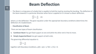
This document discusses the BVP4C method for solving boundary value problems (BVPs) using MATLAB. It begins with an introduction to differential equations, order, degree, and methods for solving first order equations. It then describes the BVP4C method, including defining the ODE function, boundary conditions function, initial guess, and mesh. As an example, it solves a second order nonlinear BVP and compares solutions using different initial guesses. Finally, it addresses using BVP4C to solve beam deflection problems.

1. A Study of BVP4C Method for
Solving Boundary Value
Problems
Department of Mathematics

2. Project Outlines
› Introduction
› Description of BVP4C Method
› Solution of Boundary Value Problems using BVP4C
› Beam Deflection Problems

3. Introduction
› Differential Equation
› Order of a Differential Equation
› Degree of the Differential Equation
› Solution of First Order Differential Equations
› Separable Equations
› Homogeneous Equations
› Exact Equations
› Linear Equations
› Initial and Boundary Value Problems

4. Introduction
› Differential Equation:
An equation containing the derivatives or differentials of one or more dependent variables with
respect to one or more independent variables is said to be a differential equation (DE).
› Order and Degree of a Differential Equation:
By order of differential equation we mean the order of the highest derivative present in the equation
and the degree of the differential equation is represented by the power of the highest order derivative
in the given differential equation:
𝑑4𝑦
𝑑𝑥4 +
𝑑2𝑦
𝑑𝑥2
2
− 3
𝑑𝑦
𝑑𝑥
+ 𝑦 = 0,
The order of differentia equation is 4 and the exponent of the highest order derivative is one. Hence,
the degree of this equation is one.
› Solution Of First Order Differential Equations:
There are few methods for solving first order Differential Equations.

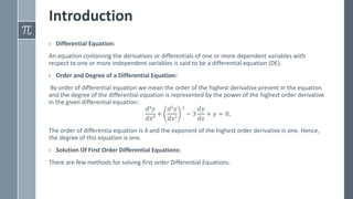
5. 1. A differential equation of form
𝑑𝑦
𝑑𝑥
=
𝑔(𝑥)
ℎ(𝑦)
is said to be separable or to have separable variables.
2. The equation P(x, y)dx + Q(x, y) dy = 0 is an exact differential equation if there exists a function u of
two variables x and y having continuous partial derivatives such that the exact differential equation
definition is separated as follows:
ux(x, y) = P(x, y) and uy(x, y) = Q(x, y),
Therefore, the general solution of the equation is u(x, y) = C.
3. If a function x has a property that f(tx,ty) = tnf(x,y) for some real number n, then f is said to be
homogeneous function of degree n.
4. A differential equation of form a1(x)
𝑑𝑦
𝑑𝑥
+ a2(x)y = g(x,y) is said to be linear equation[3].
› An Initial Value Problem (IVP) is an ordinary differential equation together with an initial condition
which specifies the value of the unknown function at a given point in the domain.
› A Boundary Value Problem (BVP) is a differential equation together with a set of additional
constraints, called the boundary conditions. A solution to a boundary value problem is a solution to the
differential equation which also satisfies the boundary conditions.

6. Description of BVP4C Method
› BVP4C
› Description
› Odefun
› Bcfun
› Solinit
› Xmesh
› Yinit-initial guess of the solution

7. Description of BVP4C Method For Solving BVPs
› BVP4C:
Solve boundary value problem — fourth-order method. BVP4C is a finite difference method code that
implement 3 step Lobatto formula. It provides continuous solutions that are fourth order accurate uniformly in
the interval of integration.
› Description:
sol = bvp4c(odefun,bcfun,solinit) integrates a system of differential equations of the form y’ = f(x,y) specified by
odefun, subject to the boundary conditions described by bcfun and the initial solution guess solinit.
› Odefun:
Functions to solve, specified as a function handle that defines the functions to be integrated. Odefun and bcfun
must accept the same number of input arguments. To code odefun, we generally use the functional signature
dydx = odefun(x,y).
› Bcfun:
To code bcfun, use the functional signature res = bcfun(ya,yb). For example, if y(a) = 1 and y(b) = 0, then the
residual value of ya(1)-1 should be 0 at the point x = a. Similarly, since y(b) = 0, the residual value of yb(1)
should be 0 at the point x =b.

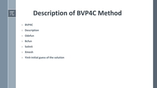
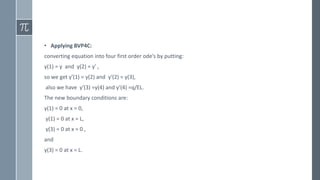
8. › Solinit:
solinit = bvpinit(x,yinit) uses the initial mesh x and initial solution guess yinit to form an initial guess of the
solution for a boundary value problem. You then can use the initial guess solinit as one of the inputs to bvp4c to
solve the boundary value problem.
› Xmesh:
Initial mesh, specified as a vector. To solve the problem on the interval [a, b], specify “x(1)” as a and “x(end)” as
b.
› Yinit-initial guess of the solution:
Forming a good initial guess of the solution to a BVP problem is perhaps the most difficult part of solving the
problem. BVP solutions are not necessarily unique, so the initial guess can be the deciding factor in which of
many solutions the solver returns.
Creating a good initial guess for the solution is more an art than a science. However, some general guidelines
include:
1. Have the initial guess satisfy the boundary conditions, since the solution is required to satisfy them as well.
2. Consider the placement of the mesh points (the x-coordinates of the initial guess of the solution).

9. Solution of Boundary Value
Problems using BVP4C
› Second Order Non-Linear Boundary Value Problem
› Applying BVP4C
› MATLAB Code for BVP
› BVP Using Different Initial Guess
› MATLAB Code for BVP
› Result Using Different Initial Guess

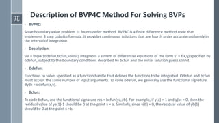
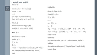
10. Solution of Boundary Value Problems Using
BVP4C
› Second Order Non-Linear Boundary Value Problem [2]
𝒅𝟐
𝒚
𝒅𝒙𝟐 + 𝒆𝒚
= 𝟎 (1)
together with Boundary Conditions y(0) = y(1) = 0.
› Applying BVP4C
converting equation(1) into two first order ode’s:
Putting y(1) = y, y(2) = y′ so we have;
y′(1) = y′, y′(2) = y′′,
Hence,
y′(1) = y(2) and y′(2) = −𝑒𝑦(1).
The new boundary conditions are:
y(0) = 0 at x = 0 and y(1) = 0 at x = 1.

11. › MATLAB Code for BVP

12. BVP Using Different Initial Guess
› Changing initial guess by [3,0]

13. Result Using Different Initial Guess

14. Beam Deflection
› The Beam is a long piece of a body that is capable to hold the load by resisting the bending. The deflection of
the beam towards in a particular direction when force is applied to it is known as Beam deflection.
𝑑4
𝑦
𝑑𝑥4 =
𝑞
𝐸𝐿
(2)
where y is the deflection. The given equation under the appropriate boundary conditions determines the
deflection of a loaded beam.
› Classification of Beam
There are two types of beam classification:
1. Cantilever Beam has got fixed support at one end while the other end is free to move.
2. Simply Supported Beam has got support at both ends.
The governing differential equation is:
𝑑4
𝑦
𝑑𝑥4 =
𝑞
𝐸𝐿
together with Boundary Conditions, y(0) = y(L) = y′′(0) = y′′(L) = 0.

15. • Applying BVP4C:
converting equation into four first order ode’s by putting:
y(1) = y and y(2) = y′ ,
so we get y′(1) = y(2) and y′(2) = y(3),
also we have y′(3) =y(4) and y′(4) =q/EL.
The new boundary conditions are:
y(1) = 0 at x = 0,
y(1) = 0 at x = L,
y(3) = 0 at x = 0 ,
and
y(3) = 0 at x = L.

16. • Matlab code for BVP

18. References
[1] Shampine, L., Gladwell, I., and Thompson, S. (2003). Solving ODEs with MATLAB. Cambridge:
Cambridge University Press. doi:10.1017/CBO9780511615542
[2] Shampine, L.F., M.W. Reichelt, and J. Kierzenka. "Solving Boundary Value Problems for Ordinary
Differential Equations in MATLAB with bvp4c." MATLAB File Exchange, 2004.
[3] Zill, Dennis G. A First Course in Differential Equations with Modeling Applications. Cengage
Learning,2012.