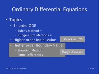
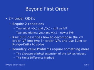
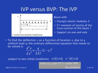
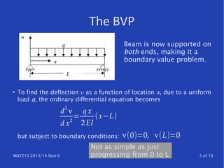
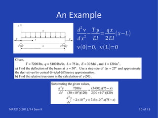
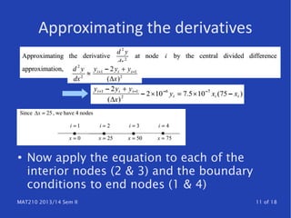
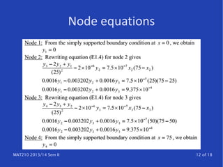
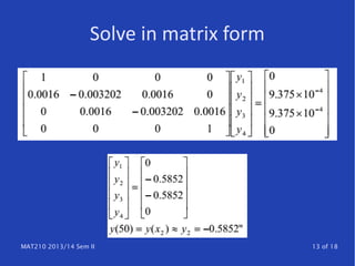
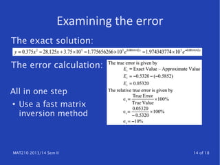
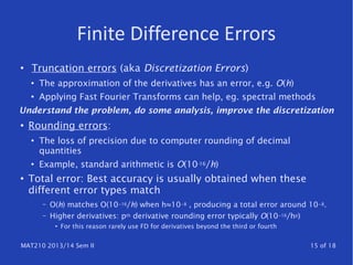
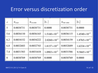
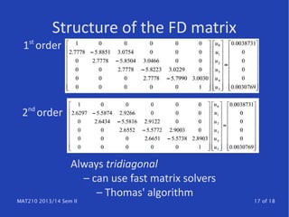
St. John's University of Tanzania
MAT210 NUMERICAL ANALYSIS
2013/14 Semester II
DIFFERENTIAL EQUATIONS
Boundary Value Problems
Kaw, Chapter 8.06-8.07
Some parts of this presentation are based on resources at
http://nm.MathForCollege.com, primarily
http://http://mathforcollege.com/nm/mtl/gen/08ode/index.html
MAT210 2013/14 Sem II 2 of 18
Ordinary Differential Equations
● Topics
●
1st order ODE
– Euler's Method 
– Runge-Kutta Methods 
● Higher order Initial Value
●
Higher order Boundary Value
– Shooting Method
– Finite Differences
Today's discussion
….Read Kaw 8.05
MAT210 2013/14 Sem II 3 of 18
Beyond First Order
●
2nd order ODE's
●
Require 2 conditions
– Two initial: y(x0) and y'(x0) – still an IVP
– Two boundaries: y(x0) and y(x1) – now a BVP
●
Kaw 8.05 describes how to decompose the 2nd
order IVP into two 1st order IVPs and use Euler or
Runge-Kutta to solve
●
Boundary Value Problems require something more
– The Shooting Method extension of the IVP techniques
– The Finite Difference Method
MAT210 2013/14 Sem II 4 of 18
IVP versus BVP: The IVP
●
To find the deflection υ as a function of location x, due to a
uniform load q, the ordinary differential equation that needs to
be solved is
subject to two initial conditions:
d
2
ν
d x2
=
q
2EI
(L−x)2
ν(0)=0, ν'(0)=0
Beam with
●
Young's elastic modulus E
●
2nd moment of inertia of the
cross-section of the beam I
●
Support on one end only
Solve as a pair of 1st order IVPs
No problem
MAT210 2013/14 Sem II 5 of 18
The BVP
●
To find the deflection υ as a function of location x, due to a uniform
load q, the ordinary differential equation becomes
but subject to boundary conditions:
d
2
ν
d x2
=
q x
2EI
(x−L)
ν(0)=0, ν(L)=0
Beam is now supported on
both ends, making it a
boundary value problem.
Not as simple as just
progressing from 0 to L
MAT210 2013/14 Sem II 6 of 18
The Shooting Method
● Why not approach the BVP using the IVP
techniques, replacing one boundary
condition with a “guess” of another initial
condition that causes the IVP solution to
“hit” the other boundary condition?
● Progressively refine the guess until it hits
● Refinement could be through interpolation
– Aha, a combination of techniques to reach the
desired objective
● This is the Shooting Method
MAT210 2013/14 Sem II 7 of 18
Summary of the Method
● Use y(x0) and a reasonable guess for y'(x0)
● Usually y'(x0)≈(y(x1)-y(x0))/(x1-x0) … FDA
●
Use Runge-Kutta to “shoot” to an
approximation for y(x1)
● If close enough, then stop, solution is done
● If not, pick another y(x0) and repeat Runge-Kutta
to get a second approximation for y(x1)
● Now use interpolation for 3rd guess
● Repeat the process until solution “hits” y(x1)
MAT210 2013/14 Sem II 8 of 18
More on the Method
●
Read the example
in Kaw Ch 8.06
●
Summarize the
steps to produce
an algorithm
●
Then it will make
more sense
MAT210 2013/14 Sem II 9 of 18
The Finite Difference Method
● Why guess and correct?
Why not feed the information from the
other boundary condition back through the
intervals?
●
That is the heart of the Finite Difference
(FD) Method
● Create a set of problems where the
subintervals share a boundary condition
● End up with a linear algebra problem
MAT210 2013/14 Sem II 10 of 18
An Example
d
2
ν
d x2
−
T y
EI
=
q x
2EI
(x−L)
ν(0)=0, ν(L)=0
MAT210 2013/14 Sem II 11 of 18
Approximating the derivatives
●
Now apply the equation to each of the
interior nodes (2 & 3) and the boundary
conditions to end nodes (1 & 4)
MAT210 2013/14 Sem II 12 of 18
Node equations
MAT210 2013/14 Sem II 13 of 18
Solve in matrix form
MAT210 2013/14 Sem II 14 of 18
Examining the error
The exact solution:
The error calculation:
All in one step
●
Use a fast matrix
inversion method
MAT210 2013/14 Sem II 15 of 18
Finite Difference Errors
●
Truncation errors (aka Discretization Errors)
●
The approximation of the derivatives has an error, e.g. O(h)
●
Applying Fast Fourier Transforms can help, eg. spectral methods
Understand the problem, do some analysis, improve the discretization
●
Rounding errors:
●
The loss of precision due to computer rounding of decimal
quantities
●
Example, standard arithmetic is O(10-16/h)
●
Total error: Best accuracy is usually obtained when these
different error types match
– O(h) matches O(10 16− /h) when h≈10 8− , producing a total error around 10 8− .
– Higher derivatives: pth derivative rounding error typically O(10 16− /hp)
●
For this reason rarely use FD for derivatives beyond the third or fourth
MAT210 2013/14 Sem II 16 of 18
Error versus discretization order
MAT210 2013/14 Sem II 17 of 18
Structure of the FD matrix
1st
order
2nd
order
Always tridiagonal
– can use fast matrix solvers
– Thomas' algorithm
MAT210 2013/14 Sem II 18 of 18
Summary
● Finite difference (FD) methods can be used
for partial differential equations, too
●
There are a wide range of FD methods,
which use different approximations for the
derivatives, different matrix techniques,
different strategies for creating intervals or
grids/meshes for PDEs
●
More at
http://www.scholarpedia.org/article/Finite_difference_method

MAT210/DiffEq/ODE/FiniteDiff 2013-14

  • 1.
    St. John's Universityof Tanzania MAT210 NUMERICAL ANALYSIS 2013/14 Semester II DIFFERENTIAL EQUATIONS Boundary Value Problems Kaw, Chapter 8.06-8.07 Some parts of this presentation are based on resources at http://nm.MathForCollege.com, primarily http://http://mathforcollege.com/nm/mtl/gen/08ode/index.html
  • 2.
    MAT210 2013/14 SemII 2 of 18 Ordinary Differential Equations ● Topics ● 1st order ODE – Euler's Method  – Runge-Kutta Methods  ● Higher order Initial Value ● Higher order Boundary Value – Shooting Method – Finite Differences Today's discussion ….Read Kaw 8.05
  • 3.
    MAT210 2013/14 SemII 3 of 18 Beyond First Order ● 2nd order ODE's ● Require 2 conditions – Two initial: y(x0) and y'(x0) – still an IVP – Two boundaries: y(x0) and y(x1) – now a BVP ● Kaw 8.05 describes how to decompose the 2nd order IVP into two 1st order IVPs and use Euler or Runge-Kutta to solve ● Boundary Value Problems require something more – The Shooting Method extension of the IVP techniques – The Finite Difference Method
  • 4.
    MAT210 2013/14 SemII 4 of 18 IVP versus BVP: The IVP ● To find the deflection υ as a function of location x, due to a uniform load q, the ordinary differential equation that needs to be solved is subject to two initial conditions: d 2 ν d x2 = q 2EI (L−x)2 ν(0)=0, ν'(0)=0 Beam with ● Young's elastic modulus E ● 2nd moment of inertia of the cross-section of the beam I ● Support on one end only Solve as a pair of 1st order IVPs No problem
  • 5.
    MAT210 2013/14 SemII 5 of 18 The BVP ● To find the deflection υ as a function of location x, due to a uniform load q, the ordinary differential equation becomes but subject to boundary conditions: d 2 ν d x2 = q x 2EI (x−L) ν(0)=0, ν(L)=0 Beam is now supported on both ends, making it a boundary value problem. Not as simple as just progressing from 0 to L
  • 6.
    MAT210 2013/14 SemII 6 of 18 The Shooting Method ● Why not approach the BVP using the IVP techniques, replacing one boundary condition with a “guess” of another initial condition that causes the IVP solution to “hit” the other boundary condition? ● Progressively refine the guess until it hits ● Refinement could be through interpolation – Aha, a combination of techniques to reach the desired objective ● This is the Shooting Method
  • 7.
    MAT210 2013/14 SemII 7 of 18 Summary of the Method ● Use y(x0) and a reasonable guess for y'(x0) ● Usually y'(x0)≈(y(x1)-y(x0))/(x1-x0) … FDA ● Use Runge-Kutta to “shoot” to an approximation for y(x1) ● If close enough, then stop, solution is done ● If not, pick another y(x0) and repeat Runge-Kutta to get a second approximation for y(x1) ● Now use interpolation for 3rd guess ● Repeat the process until solution “hits” y(x1)
  • 8.
    MAT210 2013/14 SemII 8 of 18 More on the Method ● Read the example in Kaw Ch 8.06 ● Summarize the steps to produce an algorithm ● Then it will make more sense
  • 9.
    MAT210 2013/14 SemII 9 of 18 The Finite Difference Method ● Why guess and correct? Why not feed the information from the other boundary condition back through the intervals? ● That is the heart of the Finite Difference (FD) Method ● Create a set of problems where the subintervals share a boundary condition ● End up with a linear algebra problem
  • 10.
    MAT210 2013/14 SemII 10 of 18 An Example d 2 ν d x2 − T y EI = q x 2EI (x−L) ν(0)=0, ν(L)=0
  • 11.
    MAT210 2013/14 SemII 11 of 18 Approximating the derivatives ● Now apply the equation to each of the interior nodes (2 & 3) and the boundary conditions to end nodes (1 & 4)
  • 12.
    MAT210 2013/14 SemII 12 of 18 Node equations
  • 13.
    MAT210 2013/14 SemII 13 of 18 Solve in matrix form
  • 14.
    MAT210 2013/14 SemII 14 of 18 Examining the error The exact solution: The error calculation: All in one step ● Use a fast matrix inversion method
  • 15.
    MAT210 2013/14 SemII 15 of 18 Finite Difference Errors ● Truncation errors (aka Discretization Errors) ● The approximation of the derivatives has an error, e.g. O(h) ● Applying Fast Fourier Transforms can help, eg. spectral methods Understand the problem, do some analysis, improve the discretization ● Rounding errors: ● The loss of precision due to computer rounding of decimal quantities ● Example, standard arithmetic is O(10-16/h) ● Total error: Best accuracy is usually obtained when these different error types match – O(h) matches O(10 16− /h) when h≈10 8− , producing a total error around 10 8− . – Higher derivatives: pth derivative rounding error typically O(10 16− /hp) ● For this reason rarely use FD for derivatives beyond the third or fourth
  • 16.
    MAT210 2013/14 SemII 16 of 18 Error versus discretization order
  • 17.
    MAT210 2013/14 SemII 17 of 18 Structure of the FD matrix 1st order 2nd order Always tridiagonal – can use fast matrix solvers – Thomas' algorithm
  • 18.
    MAT210 2013/14 SemII 18 of 18 Summary ● Finite difference (FD) methods can be used for partial differential equations, too ● There are a wide range of FD methods, which use different approximations for the derivatives, different matrix techniques, different strategies for creating intervals or grids/meshes for PDEs ● More at http://www.scholarpedia.org/article/Finite_difference_method