The document discusses the geometry of value functions in reinforcement learning, focusing on how understanding this geometry enhances the evaluation and transformation of value functions across various algorithms. It covers concepts like vector space representations, projection operators, and solutions to linear systems relevant in model-free learning contexts. Additionally, it presents algorithms such as gradient temporal difference methods and their applications in approximating value functions.

1. Value Function Geometry and Gradient TD
Ashwin Rao
Stanford University, ICME
October 27, 2018
Ashwin Rao (Stanford) Value Function Geometry October 27, 2018 1 / 19

2. Overview
1 Motivation and Notation
2 Geometric/Vector Space Representation of Value Functions
3 Solutions with Linear System Formulations
4 Residual Gradient TD
5 Gradient TD
Ashwin Rao (Stanford) Value Function Geometry October 27, 2018 2 / 19

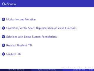
3. Motivation for understanding Value Function Geometry
Helps us better understand transformations of Value Functions (VFs)
Across the various DP and RL algorithms
Particularly helps when VFs are approximated, esp. with linear approx
Provides insights into stability and convergence
Particularly when dealing with the “Deadly Triad”
Deadly Triad := [Bootstrapping, Func Approx, Off-Policy]
Leads us to Gradient TD
Ashwin Rao (Stanford) Value Function Geometry October 27, 2018 3 / 19

4. Notation
Assume state space S consists of n states: {s1, s2, . . . , sn}
Action space A consisting of finite number of actions
This exposition extends easily to continuous state/action spaces too
This exposition is for a fixed (often stochastic) policy denoted π(a|s)
VF for a policy π is denoted as vπ : S → R
m feature functions φ1, φ2, . . . , φm : S → R
Feature vector for a state s ∈ S denoted as φ(s) ∈ Rm
For linear function approximation of VF with weights
w = (w1, w2, . . . , wm), VF vw : S → R is defined as:
vw(s) = wT
· φ(s) =
m
j=1
wj · φj (s) for any s ∈ S
µπ : S → [0, 1] denotes the states’ probability distribution under π
Ashwin Rao (Stanford) Value Function Geometry October 27, 2018 4 / 19

5. VF Vector Space and VF Linear Approximations
n-dimensional space, with each dim corresponding to a state in S
A vector in this space is a specific VF (typically denoted v): S → R
Wach dimension’s coordinate is the VF for that dimension’s state
Coordinates of vector vπ for policy π are: [vπ(s1), vπ(s2), . . . , vπ(sn)]
Consider m vectors where jth vector is: [φj (s1), φj (s2), . . . , φj (sn)]
These m vectors are the m columns of n × m matrix Φ = [φj (si )]
Their span represents an m-dim subspace within this n-dim space
Spanned by the set of all w = [w1, w2, . . . , wm] ∈ Rm
Vector vw = Φ · w in this subspace has coordinates
[vw(s1), vw(s2), . . . , vw(sn)]
Vector vw is fully specified by w (so we often say w to mean vw)
Ashwin Rao (Stanford) Value Function Geometry October 27, 2018 5 / 19

6. Some more notation
Denote r(s, a) as the Expected Reward upon action a in state s
Denote p(s, s , a) as the probability of transition s → s upon action a
Define
R(s) =
a∈A
π(a|s) · r(s, a)
P(s, s ) =
a∈A
π(a|s) · p(s, s , a)
Denote R as the vector [R(s1), R(s2), . . . , R(sn)]
Denote P as the matrix [P(si , si )], 1 ≤ i, i ≤ n
Denote γ as the MDP discount factor
Ashwin Rao (Stanford) Value Function Geometry October 27, 2018 6 / 19

7. Bellman operator Bπ
Bellman operator Bπ for policy π operating on VF vector v defined as:
Bπv = R + γP · v
Note that vπ is the fixed point of operator Bπ (meaning Bπvπ = vπ)
If we start with an arbitrary VF vector v and repeatedly apply Bπ, by
Contraction Mapping Theorem, we will reach the fixed point vπ
This is the Dynamic Programming Policy Evaluation algorithm
Monte Carlo without func approx also converges to vπ (albeit slowly)
Ashwin Rao (Stanford) Value Function Geometry October 27, 2018 7 / 19

8. Projection operator ΠΦ
Firs we define “distance” d(v1, v2) between VF vectors v1, v2
Weighted by µπ across the n dimensions of v1, v2
d(v1, v2) =
n
i=1
µπ(si ) · (v1(si ) − v2(si ))2
= (v1 − v2)T
· D · (v1 − v2)
where D is the square diagonal matrix consisting of µπ(si ), 1 ≤ i ≤ n
Projection operator for subspace spanned by Φ is denoted as ΠΦ
ΠΦ performs an orthogonal projection of VF vector v on subspace Φ
So we need to minimize d(v, ΠΦv)
This is a weighted least squares regression with solution:
w = (ΦT
· D · Φ)−1
· ΦT
· D · v
So, the Projection operator ΠΦ can be written as:
ΠΦ = Φ · (ΦT
· D · Φ)−1
· ΦT
· D
Ashwin Rao (Stanford) Value Function Geometry October 27, 2018 8 / 19

9. 4 VF vectors of interest in the Φ subspace
Note: We will refer to the Φ-subspace VF vectors by their weights w
1 Projection of vπ: wπ = arg minw d(vπ, vw)
This is the VF we seek when doing linear function approximation
Because it is the VF vector “closest” to vπ in the Φ subspace
Monte-Carlo with linear func approx will (slowly) converge to wπ
2 Bellman Error (BE)-minimizing: wBE = arg minw d(Bπvw, vw)
This is the solution to a linear system (covered later)
In model-free setting, Residual Gradient TD Algorithm (covered later)
Cannot learn if we can only access features, and not underlying states
Ashwin Rao (Stanford) Value Function Geometry October 27, 2018 9 / 19

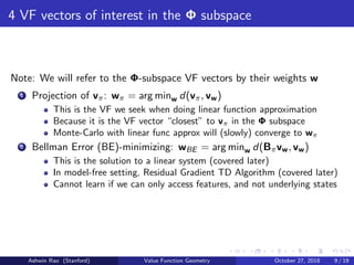
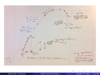
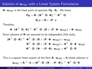
10. 4 VF vectors of interest in the Φ subspace (continued)
3 Projected Bellman Error (PBE)-minimizing:
wPBE = arg minw d((ΠΦ · Bπ)vw, vw)
The minimum is 0, i.e., Φ · wPBE is the fixed point of operator ΠΦ · Bπ
This fixed point is the solution to a linear system (covered later)
Alternatively, if we start with an arbitrary vw and repeatedly apply
ΠΦ · Bπ, we will converge to Φ · wPBE
This is a DP-like process with approximation - repeatedly thrown out of
the Φ subspace (applying Bellman operator Bπ), followed by landing
back in the Φ subspace (applying Projection operator ΠΦ)
In model-free setting, Gradient TD Algorithms (covered later)
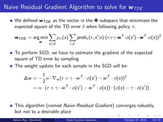
4 Temporal Difference Error (TDE)-minimizing:
wTDE = arg minw Eπ[δ2]
δ is the TD error
Minimizes the expected square of the TD error when following policy π
Naive Residual Gradient TD Algorithm (covered later)
Ashwin Rao (Stanford) Value Function Geometry October 27, 2018 10 / 19

11. Ashwin Rao (Stanford) Value Function Geometry October 27, 2018 11 / 19

12. Solution of wBE with a Linear System Formulation
wBE = arg min
w
d(vw, R + γP · vw)
= arg min
w
d(Φ · w, R + γP · Φ · w)
= arg min
w
d(Φ · w − γP · Φ · w, R)
= arg min
w
d((Φ − γP · Φ) · w, R)
This is a weighted least-squares linear regression of R versus Φ − γP · Φ
with weights µπ, whose solution is:
wBE = ((Φ − γP · Φ)T
· D · (Φ − γP · Φ))−1
· (Φ − γP · Φ)T
· D · R
Ashwin Rao (Stanford) Value Function Geometry October 27, 2018 12 / 19

13. Solution of wPBE with a Linear System Formulation
Φ · wPBE is the fixed point of operator ΠΦ · Bπ. We know:
ΠΦ = Φ · (ΦT
· D · Φ)−1
· ΦT
· D
Bπv = R + γP · v
Therefore,
Φ · (ΦT
· D · Φ)−1
· ΦT
· D · (R + γP · Φ · wPBE ) = Φ · wPBE
Since columns of Φ are assumed to be independent (full rank),
(ΦT
· D · Φ)−1
· ΦT
· D · (R + γP · Φ · wPBE ) = wPBE
ΦT
· D · (R + γP · Φ · wPBE ) = ΦT
· D · Φ · wPBE
ΦT
· D · (Φ − γP · Φ) · wPBE = ΦT
· D · R
This is a square linear system of the form A · wPBE = b whose solution is:
wPBE = A−1
· b = (ΦT
· D · (Φ − γP · Φ))−1
· ΦT
· D · R
Ashwin Rao (Stanford) Value Function Geometry October 27, 2018 13 / 19

14. Model-Free Learning of wPBE
How do we construct matrix A = ΦT · D · (Φ − γP · Φ) and vector
b = ΦT · D · R without a model?
Following policy π, each time we perform a model-free transition from
s to s getting reward r, we get a sample estimate of A and b
Estimate of A is the outer-product of vectors φ(s) and φ(s) − γ · φ(s )
Estimate of b is scalar r times vector φ(s)
Average these estimates across many such model-free transitions
This algorithm is called Least Squares Temporal Difference (LSTD)
Alternative: Semi-Gradient Temporal Difference (TD) descent
This semi-gradient descent converges to wPBE with weight updates:
∆w = α · (r + γ · wT
· φ(s ) − wT
· φ(s)) · φ(s)
r + γ · wT · φ(s ) − wT · φ(s) is the TD error, denoted δ
Ashwin Rao (Stanford) Value Function Geometry October 27, 2018 14 / 19

15. Naive Residual Gradient Algorithm to solve for wTDE
We defined wTDE as the vector in the Φ subspace that minimizes the
expected square of the TD error δ when following policy π.
wTDE = arg min
w
s∈S
µπ(s)
r,s
probπ(r, s |s)·(r+γ·wT
·φ(s )−wT
·φ(s))2
To perform SGD, we have to estimate the gradient of the expected
square of TD error by sampling
The weight update for each sample in the SGD will be:
∆w = −
1
2
α · w (r + γ · wT
· φ(s ) − wT
· φ(s))2
= α · (r + γ · wT
· φ(s ) − wT
· φ(s)) · (φ(s) − γ · φ(s ))
This algorithm (named Naive Residual Gradient) converges robustly,
but not to a desirable place
Ashwin Rao (Stanford) Value Function Geometry October 27, 2018 15 / 19

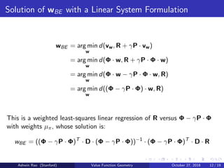
16. Residual Gradient Algorithm to solve for wBE
We defined wBE as the vector in the Φ subspace that minimizes BE
But BE for a state is the expected TD error in that state
So we want to do SGD with gradient of square of expected TD error
∆w = −
1
2
α · w (Eπ[δ])2
= −α · Eπ[r + γ · wT
· φ(s ) − wT
· φ(s)] · w Eπ[δ]
= α · (Eπ[r + γ · wT
· φ(s )] − wT
· φ(s)) · (φ(s) − γ · Eπ[φ(s )])
This is called the Residual Gradient algorithm
Requires two independent samples of s transitioning from s
In that case, converges to wBE robustly (even for non-linear approx)
But it is slow, and doesn’t converge to a desirable place
Cannot learn if we can only access features, and not underlying states
Ashwin Rao (Stanford) Value Function Geometry October 27, 2018 16 / 19

17. Gradient TD Algorithms to solve for wPBE
For on-policy linear func approx, semi-gradient TD works
For non-linear func approx or off-policy, we need Gradient TD
GTD: The original Gradient TD algorithm
GTD-2: Second-generation GTD
TDC: TD with Gradient correction
We need to set up the loss function whose gradient will drive SGD
wPBE = arg minw d(ΠΦBπvw, vw) = arg minw d(ΠΦBπvw, ΠΦvw)
So we define the loss function (denoting Bπvw − vw as δw) as:
L(w) = (ΠΦδw)T
· D · (ΠΦδw) = δw
T
· ΠT
Φ · D · ΠΦ · δw
= δw
T
·(Φ·(ΦT
·D·Φ)−1
·ΦT
·D)T
·D·(Φ·(ΦT
·D·Φ)−1
·ΦT
·D)·δw
= δw
T
·(D·Φ·(ΦT
·D·Φ)−1
·ΦT
)·D·(Φ·(ΦT
·D·Φ)−1
·ΦT
·D)·δw
= (δw
T
·D·Φ)·(ΦT
·D·Φ)−1
·(ΦT
·D·Φ)·(ΦT
·D·Φ)−1
·(ΦT
·D·δw)
= (ΦT
· D · δw)T
· (ΦT
· D · Φ)−1
· (ΦT
· D · δw)
Ashwin Rao (Stanford) Value Function Geometry October 27, 2018 17 / 19

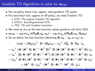
18. TDC Algorithm to solve for wPBE
We derive the TDC Algorithm based on wL(w)
wL(w) = 2 · ( w(ΦT
· D · δw)T
) · (ΦT
· D · Φ)−1
· (ΦT
· D · δw)
Now we express each of these 3 terms as expectations of model-free
transitions s
µ
−→ (r, s ), denoting r + γ · wT · φ(s ) − wT · φ(s) as δ
ΦT · D · δw = E[δ · φ(s)]
w(ΦT · D · δw)T = w(E[δ · φ(s)])T = E[( wδ) · φ(s)T ] =
E[(γ · φ(s ) − φ(s)) · φ(s)T ]
ΦT · D · Φ = E[φ(s) · φ(s)T ]
Substituting, we get:
wL(w) = 2 · E[(γ · φ(s ) − φ(s)) · φ(s)T
] · E[φ(s) · φ(s)T
]−1
· E[δ · φ(s)]
Ashwin Rao (Stanford) Value Function Geometry October 27, 2018 18 / 19

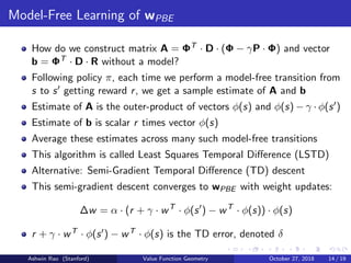
19. Weight Updates of TDC Algorithm
∆w = −
1
2
α · wL(w)
= α · E[(φ(s) − γ · φ(s )) · φ(s)T
] · E[φ(s) · φ(s)T
]−1
· E[δ · φ(s)]
= α · (E[φ(s) · φ(s)T
] − γ · E[φ(s ) · φ(s)T
]) · E[φ(s) · φ(s)T
]−1
· E[δ · φ(s)]
= α · (E[δ · φ(s)] − γ · E[φ(s ) · φ(s)T
] · E[φ(s) · φ(s)T
]−1
· E[δ · φ(s)])
= α · (E[δ · φ(s)] − γ · E[φ(s ) · φ(s)T
] · θ)
where θ = E[φ(s) · φ(s)T ]−1 · E[δ · φ(s)] is the solution to a weighted
least-squares linear regression of Bπv − v against Φ, with weights as µπ.
Cascade Learning: Update both w and θ (θ converging faster)
∆w = α · δ · φ(s) − α · γ · φ(s ) · (θT · φ(s))
∆θ = β · (δ − θT · φ(s)) · φ(s)
Note: θT · φ(s) operates as estimate of TD error δ for current state s
Ashwin Rao (Stanford) Value Function Geometry October 27, 2018 19 / 19