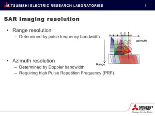
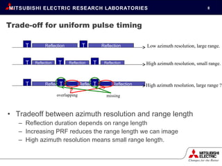
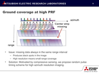
High resolution SAR imaging using random pulse timing Dehong Liu IGARSS’ 2011  Vancouver, CANADA Joint work with  Petros Boufounos.
Outline Overview of synthetic aperture radar (SAR)  Compressive sensing (CS) and random pulse timing  Iterative reconstruction algorithm Imaging results with synthetic data Conclusion and future work
Overview of SAR
Synthetic Aperture Radar (SAR) Ground Range v azimuth azimuth Reflection duration depends on range length.
Strip-map SAR: uniform pulsing Ground azimuth Range azimuth v
Data acquisition and image formation SAR acquisition follows linear model y   =     x ,  where  y :   Received Data,  x :   Ground reflectivity,     :   Acquisition function determined by SAR parameters, for example, pulse shape, PRF, SAR platform trajectory, etc.  Image formation: determine  x   given  y   and    .  Range Doppler Algorithm Chirp Scaling Algorithm Specific to Chirp Pulses
SAR imaging resolution Range resolution Determined by pulse frequency bandwidth Azimuth resolution Determined by Doppler bandwidth Requiring high Pulse Repetition Frequency (PRF) azimuth Range
Trade-off for uniform pulse timing Tradeoff between azimuth resolution and range length Reflection duration depends on range length Increasing PRF reduces the range length we can image High azimuth resolution means small range length. Low azimuth resolution, large range. High azimuth resolution, small range. High azimuth resolution, large range ? T Reflection T Reflection T Reflection T Reflection T Reflection overlapping missing T Reflection T T Reflection Reflection
Ground coverage at high PRF Issue: missing data always in the same range interval Produces black spots in the image High resolution means small range coverage Solution: Motivated by compressive sensing, we propose random pulse timing scheme for high azimuth resolution imaging. azimuth range
Compressive sensing and random pulse timing
Compressive sensing vs. Nyquist sampling Nyquist / Shannon sampling theory Sample at twice the signal bandwidth  Compressive sensing  Sparse / compressible signal Sub-Nyquist sampling rate Reconstruct using the sparsity model
Compressive sensing and reconstruction CS measurement Reconstruction Signal model:  Provides prior information; allows undersampling; Randomness:  Provides robustness/stability;  Non-linear reconstruction:  Incorporates information through computation. measurements sparse signal Non-zeroes Φ measurements sparse signal Φ
Connection between CS and SAR imaging Question: Can we apply compressive sensing to SAR imaging?  SAR imaging CS y   =     x Data acquisition Random projection measurements y Radar echo CS measurements x  Ground reflectivity Sparse signal    Acquisition function determined by SAR parameters Random projection matrix x | y ,      Image formation Sparse signal reconstruction
Random pulse timing Randomized pulsing interval azimuth range Randomized timing  mixes missing data
Iterative reconstruction algorithm
Iterative reconstruction algorithm Note: Fast computation of     and     H  always speeds up the algorithm.
Efficient computation   Azimuth FFT Chirp Scaling (differential RCMC) Range FFT Bulk RCMC, RC, SRC Range IFFT F r F a S -1 F r -1 P a H F a -1 Azimuth Compression/ Phase Correction Azimuth IFFT Chirp Scaling Algorithm Computation of    follows reverse path Computation as efficient as CSA y P r H B -1 R -1
Imaging results with synthetic data
Experiment w/ synthetic data SAR parameters: RADARSAT-1 Ground reflectivity: Complex valued image of Vancouver area Quasi-random pulsing: Oversample 6 times in azimuth, and randomly select half samples to transmit pulses, resulting 3 times effective azimuth oversampling.  Randomization ensures missing data well distributed
Radar  Image Radar  Raw Data Ground Classic Pulsing low PRF Random Pulsing high PRF + missing data Image with low azimuth resolution Image with high azimuth resolution Radar data acquisition Forward process Standard Algorithm Iterative Algorithm Simulated Ground Reflectivity (high-resolution)
Zoom-in imaging results True Ground Reflectivity Uniform pulsing, Small PRF, Small Doppler Bandwidth Random pulsing, High PRF, Large Doppler Bandwidth
Conclusion and future work
Conclusion Proposed random pulse timing scheme with high average PRF for high resolution SAR imaging.  Utilized iterative non-linear CS reconstruction method to reconstruct SAR image.  Achieved high azimuth resolution imaging results without losing range coverage.  Noise and nadir echo interference issues.  Computational speed.  Future work

4-IGARSS_2011_v4.ppt

  • 1.
    High resolution SARimaging using random pulse timing Dehong Liu IGARSS’ 2011 Vancouver, CANADA Joint work with Petros Boufounos.
  • 2.
    Outline Overview ofsynthetic aperture radar (SAR) Compressive sensing (CS) and random pulse timing Iterative reconstruction algorithm Imaging results with synthetic data Conclusion and future work
  • 3.
  • 4.
    Synthetic Aperture Radar(SAR) Ground Range v azimuth azimuth Reflection duration depends on range length.
  • 5.
    Strip-map SAR: uniformpulsing Ground azimuth Range azimuth v
  • 6.
    Data acquisition andimage formation SAR acquisition follows linear model y =  x , where y : Received Data, x : Ground reflectivity,  : Acquisition function determined by SAR parameters, for example, pulse shape, PRF, SAR platform trajectory, etc. Image formation: determine x given y and  . Range Doppler Algorithm Chirp Scaling Algorithm Specific to Chirp Pulses
  • 7.
    SAR imaging resolutionRange resolution Determined by pulse frequency bandwidth Azimuth resolution Determined by Doppler bandwidth Requiring high Pulse Repetition Frequency (PRF) azimuth Range
  • 8.
    Trade-off for uniformpulse timing Tradeoff between azimuth resolution and range length Reflection duration depends on range length Increasing PRF reduces the range length we can image High azimuth resolution means small range length. Low azimuth resolution, large range. High azimuth resolution, small range. High azimuth resolution, large range ? T Reflection T Reflection T Reflection T Reflection T Reflection overlapping missing T Reflection T T Reflection Reflection
  • 9.
    Ground coverage athigh PRF Issue: missing data always in the same range interval Produces black spots in the image High resolution means small range coverage Solution: Motivated by compressive sensing, we propose random pulse timing scheme for high azimuth resolution imaging. azimuth range
  • 10.
    Compressive sensing andrandom pulse timing
  • 11.
    Compressive sensing vs.Nyquist sampling Nyquist / Shannon sampling theory Sample at twice the signal bandwidth Compressive sensing Sparse / compressible signal Sub-Nyquist sampling rate Reconstruct using the sparsity model
  • 12.
    Compressive sensing andreconstruction CS measurement Reconstruction Signal model: Provides prior information; allows undersampling; Randomness: Provides robustness/stability; Non-linear reconstruction: Incorporates information through computation. measurements sparse signal Non-zeroes Φ measurements sparse signal Φ
  • 13.
    Connection between CSand SAR imaging Question: Can we apply compressive sensing to SAR imaging? SAR imaging CS y =  x Data acquisition Random projection measurements y Radar echo CS measurements x Ground reflectivity Sparse signal  Acquisition function determined by SAR parameters Random projection matrix x | y ,  Image formation Sparse signal reconstruction
  • 14.
    Random pulse timingRandomized pulsing interval azimuth range Randomized timing mixes missing data
  • 15.
  • 16.
    Iterative reconstruction algorithmNote: Fast computation of  and  H always speeds up the algorithm.
  • 17.
    Efficient computation  Azimuth FFT Chirp Scaling (differential RCMC) Range FFT Bulk RCMC, RC, SRC Range IFFT F r F a S -1 F r -1 P a H F a -1 Azimuth Compression/ Phase Correction Azimuth IFFT Chirp Scaling Algorithm Computation of  follows reverse path Computation as efficient as CSA y P r H B -1 R -1
  • 18.
    Imaging results withsynthetic data
  • 19.
    Experiment w/ syntheticdata SAR parameters: RADARSAT-1 Ground reflectivity: Complex valued image of Vancouver area Quasi-random pulsing: Oversample 6 times in azimuth, and randomly select half samples to transmit pulses, resulting 3 times effective azimuth oversampling. Randomization ensures missing data well distributed
  • 20.
    Radar ImageRadar Raw Data Ground Classic Pulsing low PRF Random Pulsing high PRF + missing data Image with low azimuth resolution Image with high azimuth resolution Radar data acquisition Forward process Standard Algorithm Iterative Algorithm Simulated Ground Reflectivity (high-resolution)
  • 21.
    Zoom-in imaging resultsTrue Ground Reflectivity Uniform pulsing, Small PRF, Small Doppler Bandwidth Random pulsing, High PRF, Large Doppler Bandwidth
  • 22.
    Zoom-in imaging resultsTrue Ground Reflectivity Uniform pulsing, Small PRF, Small Doppler Bandwidth Random pulsing, High PRF, Large Doppler Bandwidth
  • 23.
  • 24.
    Conclusion Proposed randompulse timing scheme with high average PRF for high resolution SAR imaging. Utilized iterative non-linear CS reconstruction method to reconstruct SAR image. Achieved high azimuth resolution imaging results without losing range coverage. Noise and nadir echo interference issues. Computational speed. Future work

Editor's Notes