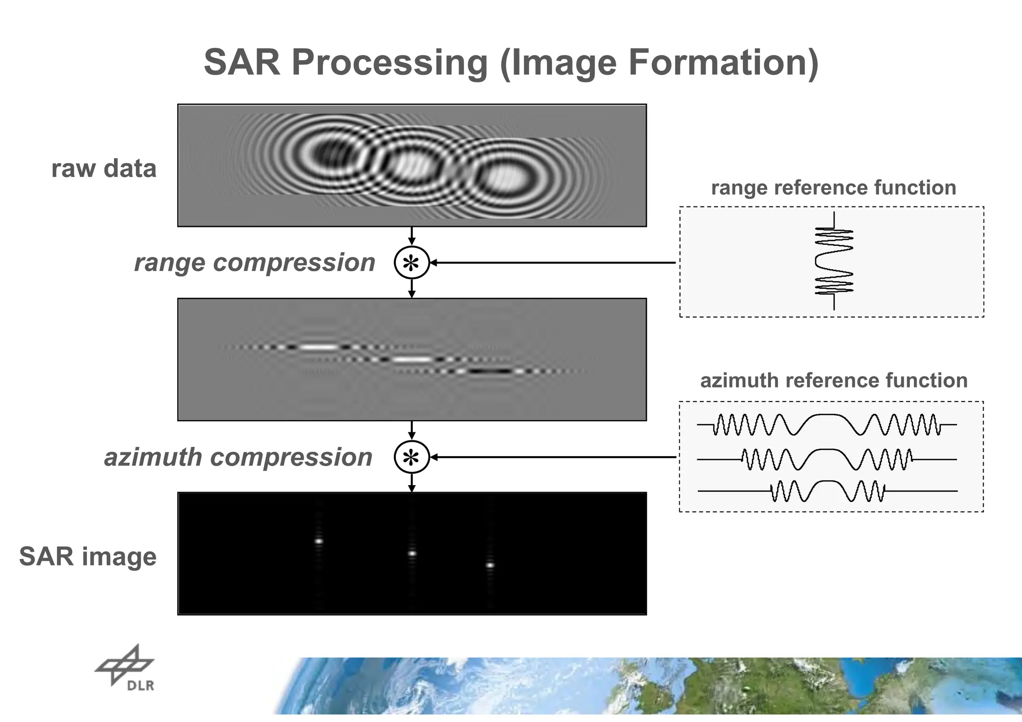
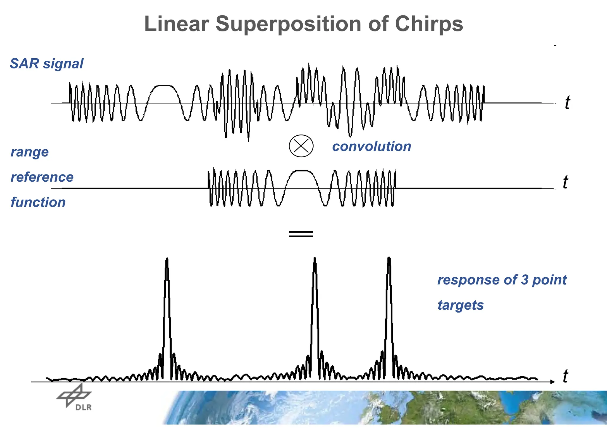
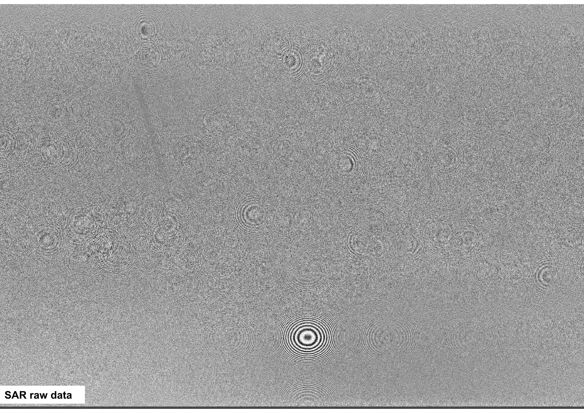
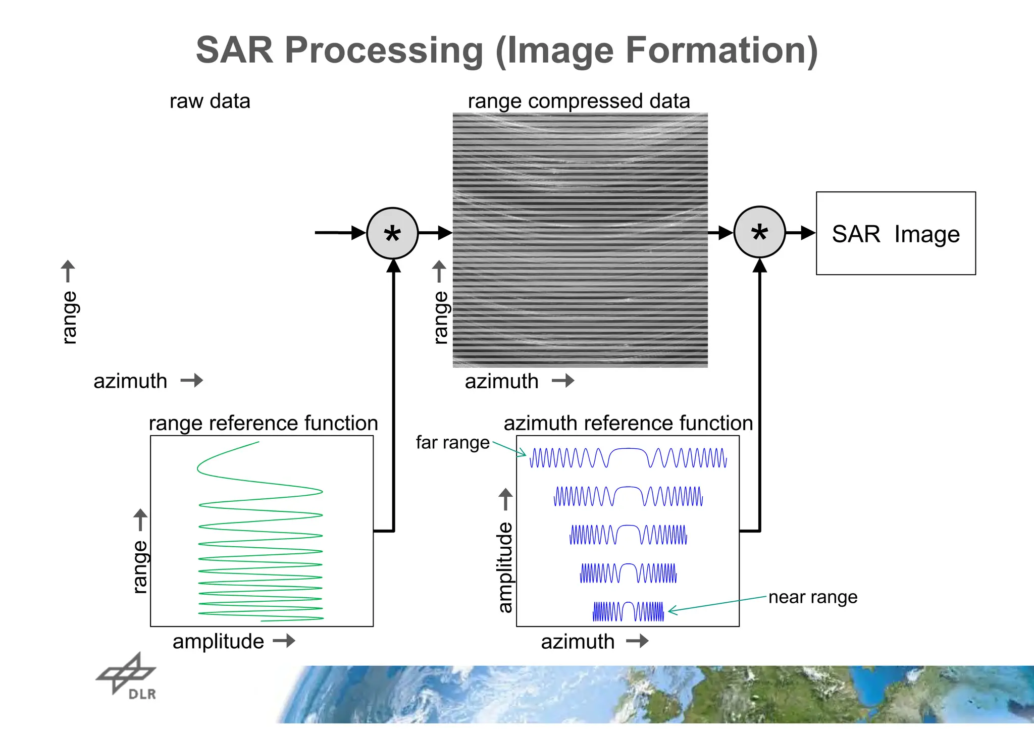
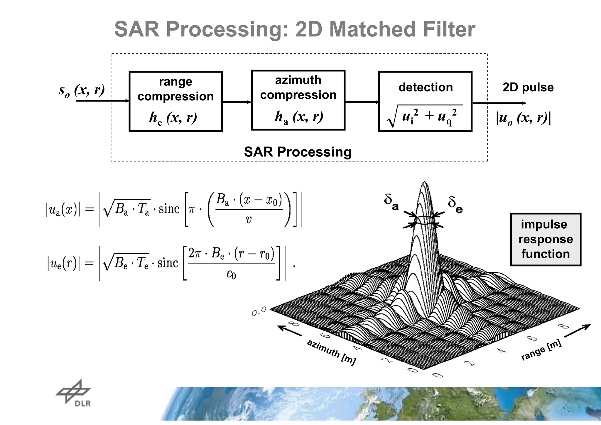
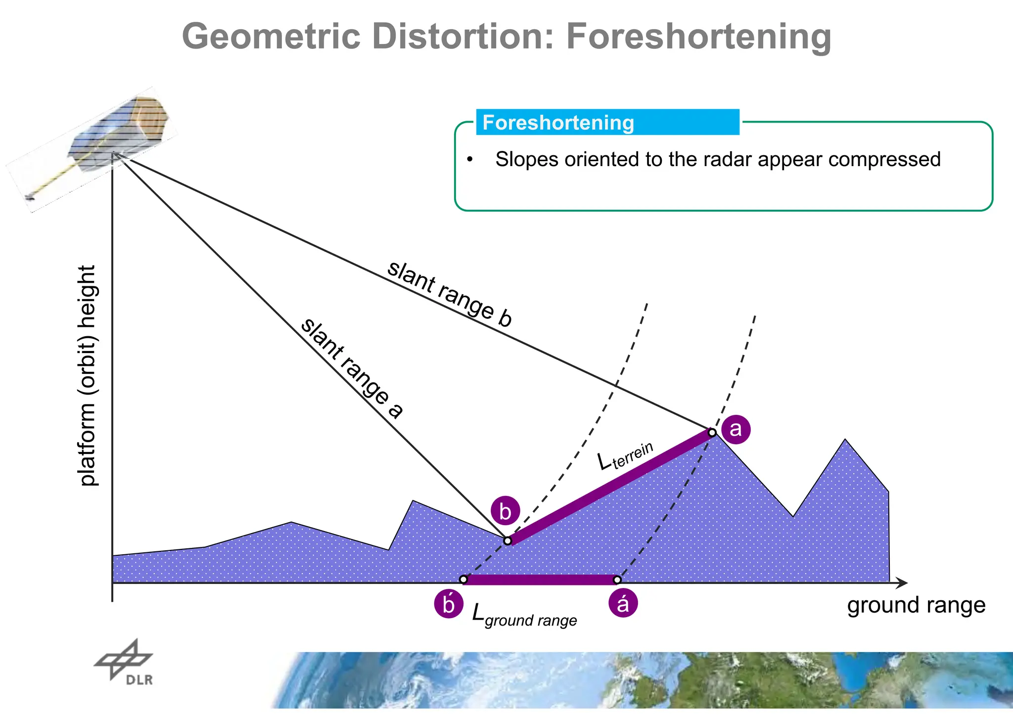
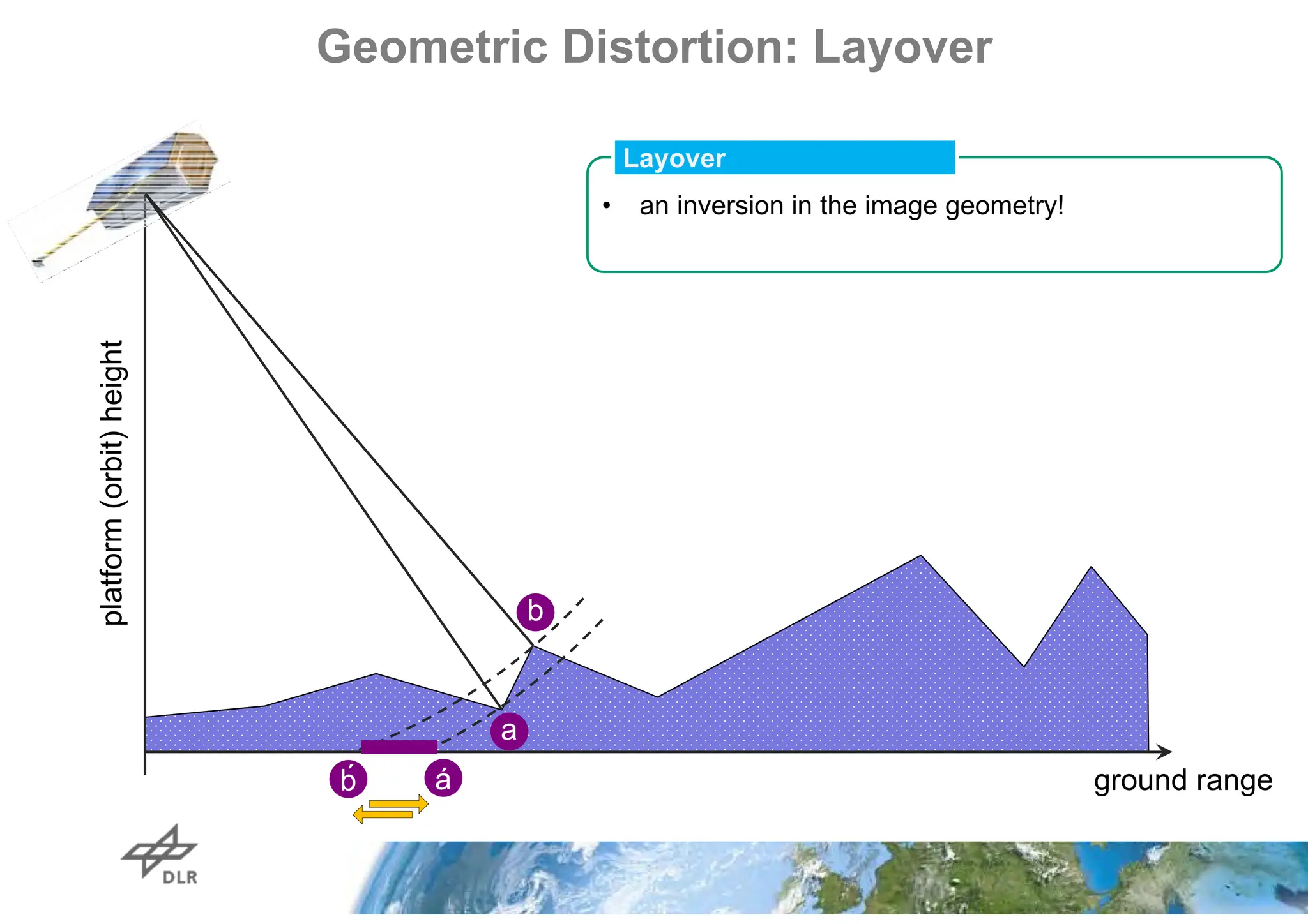
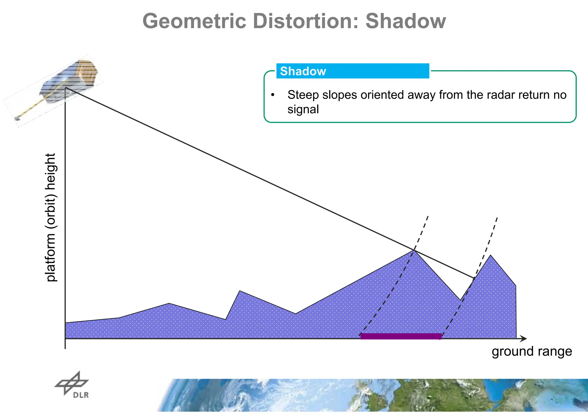
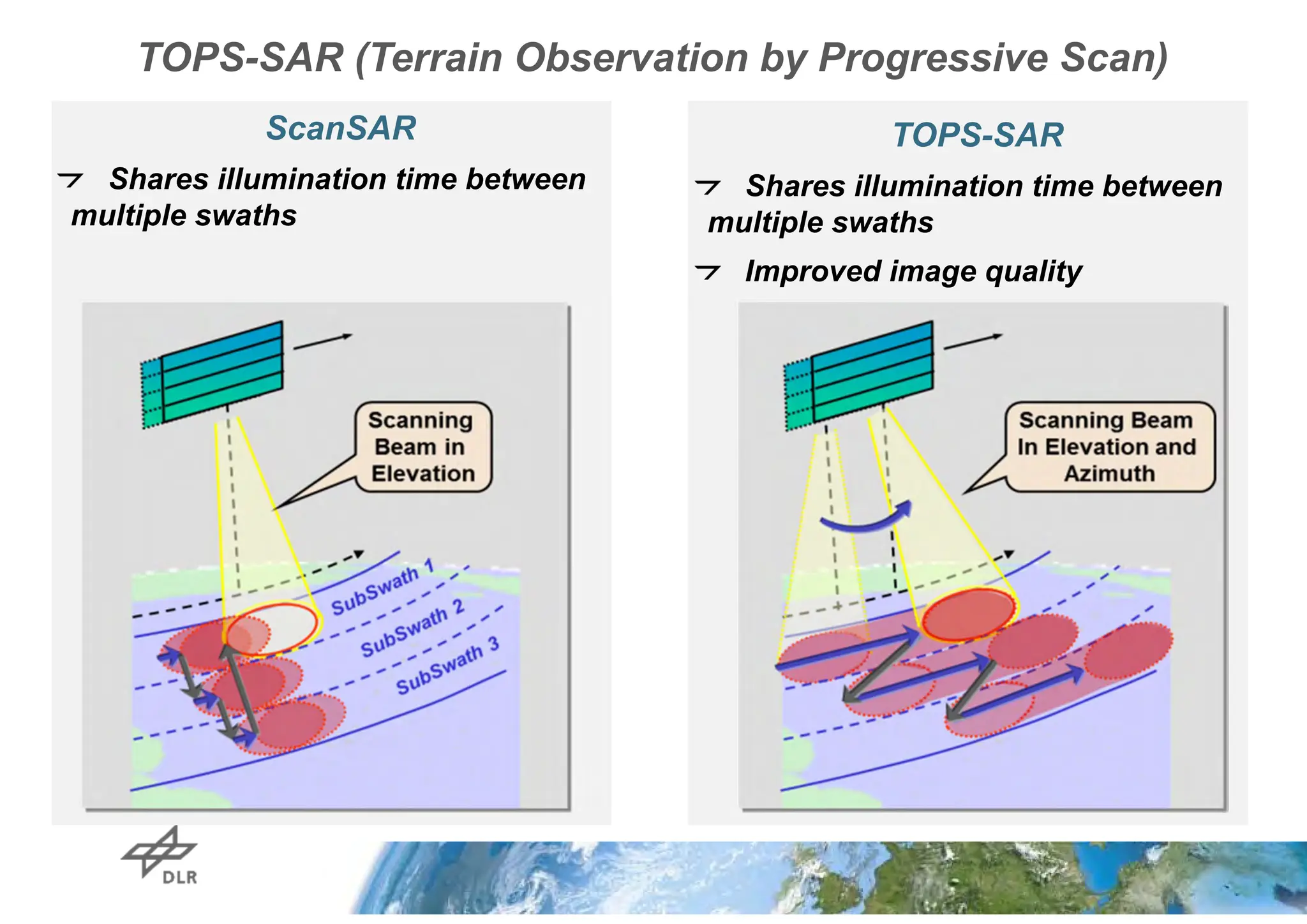
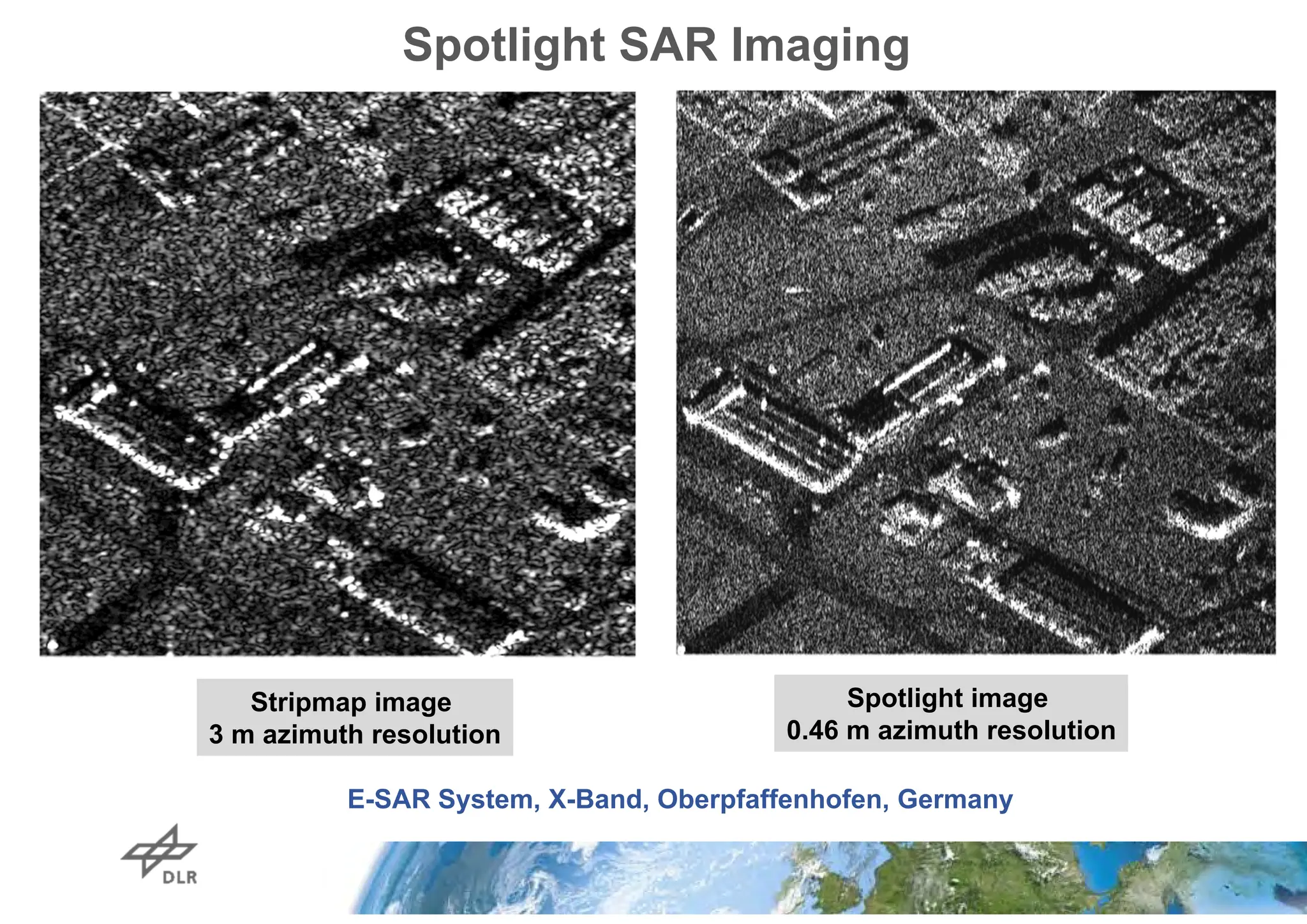
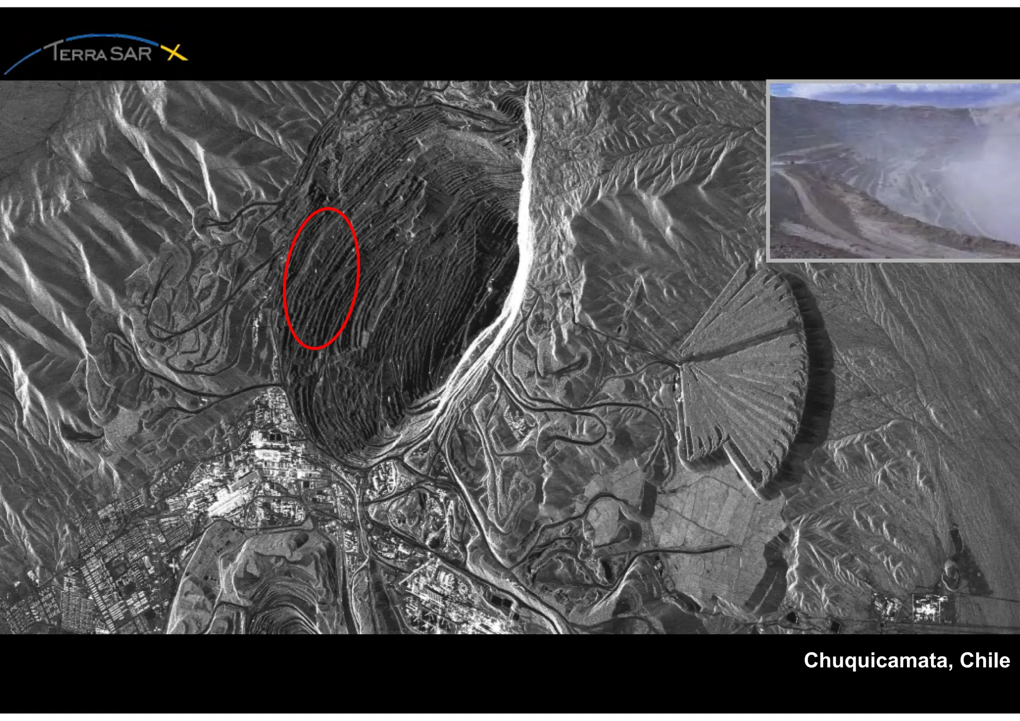
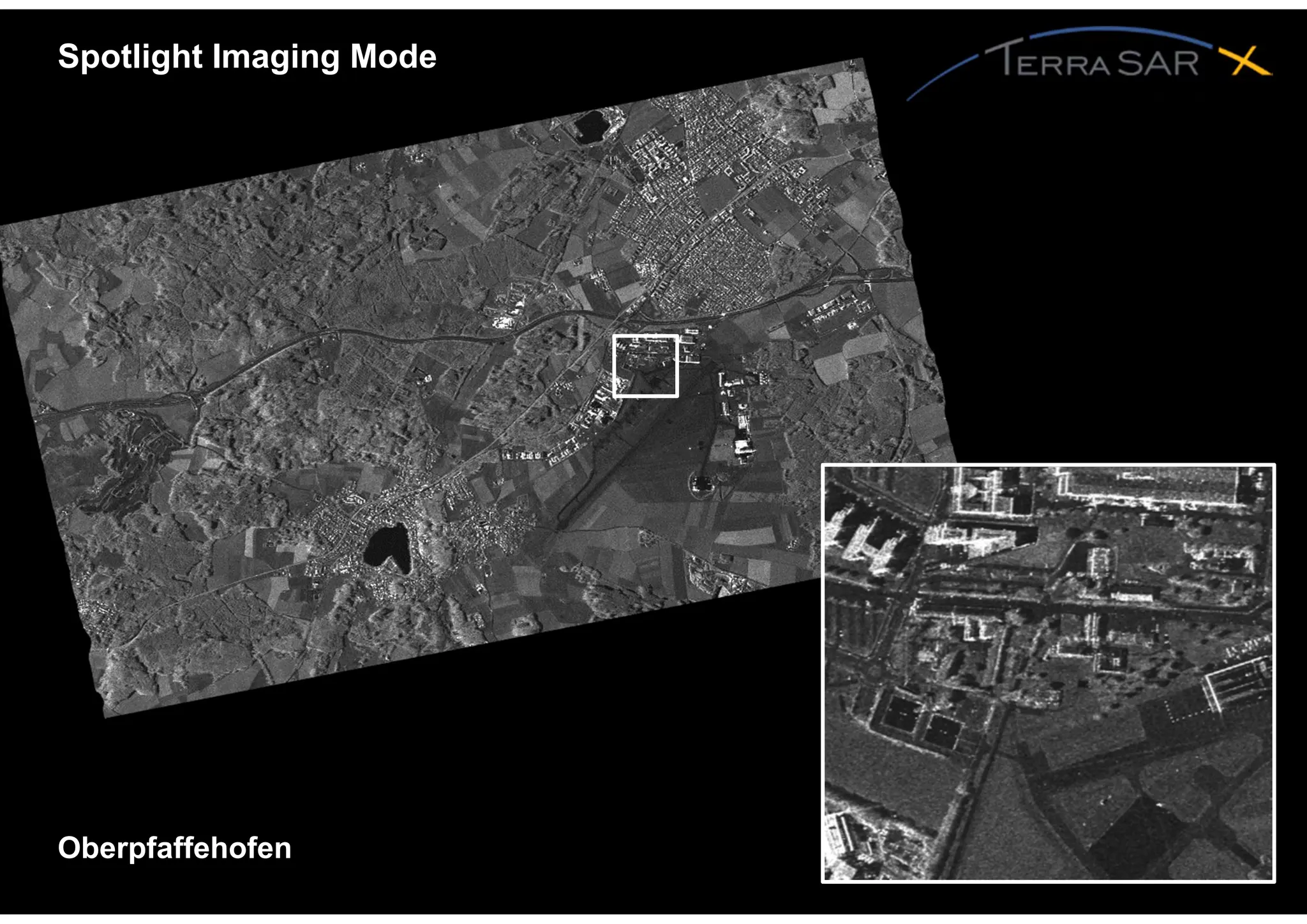
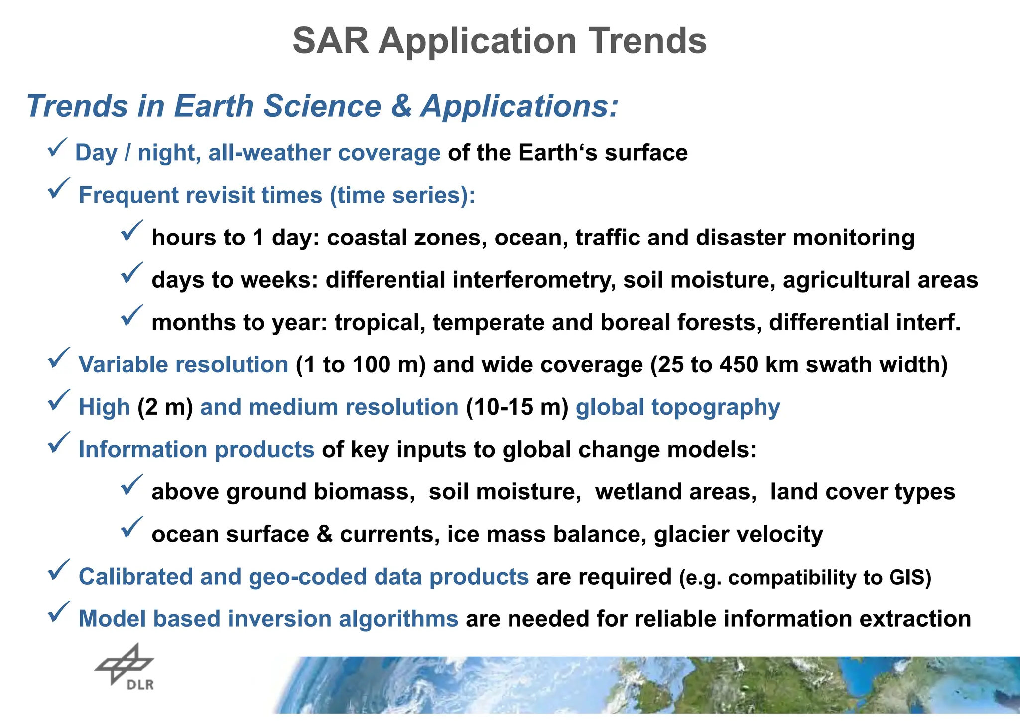
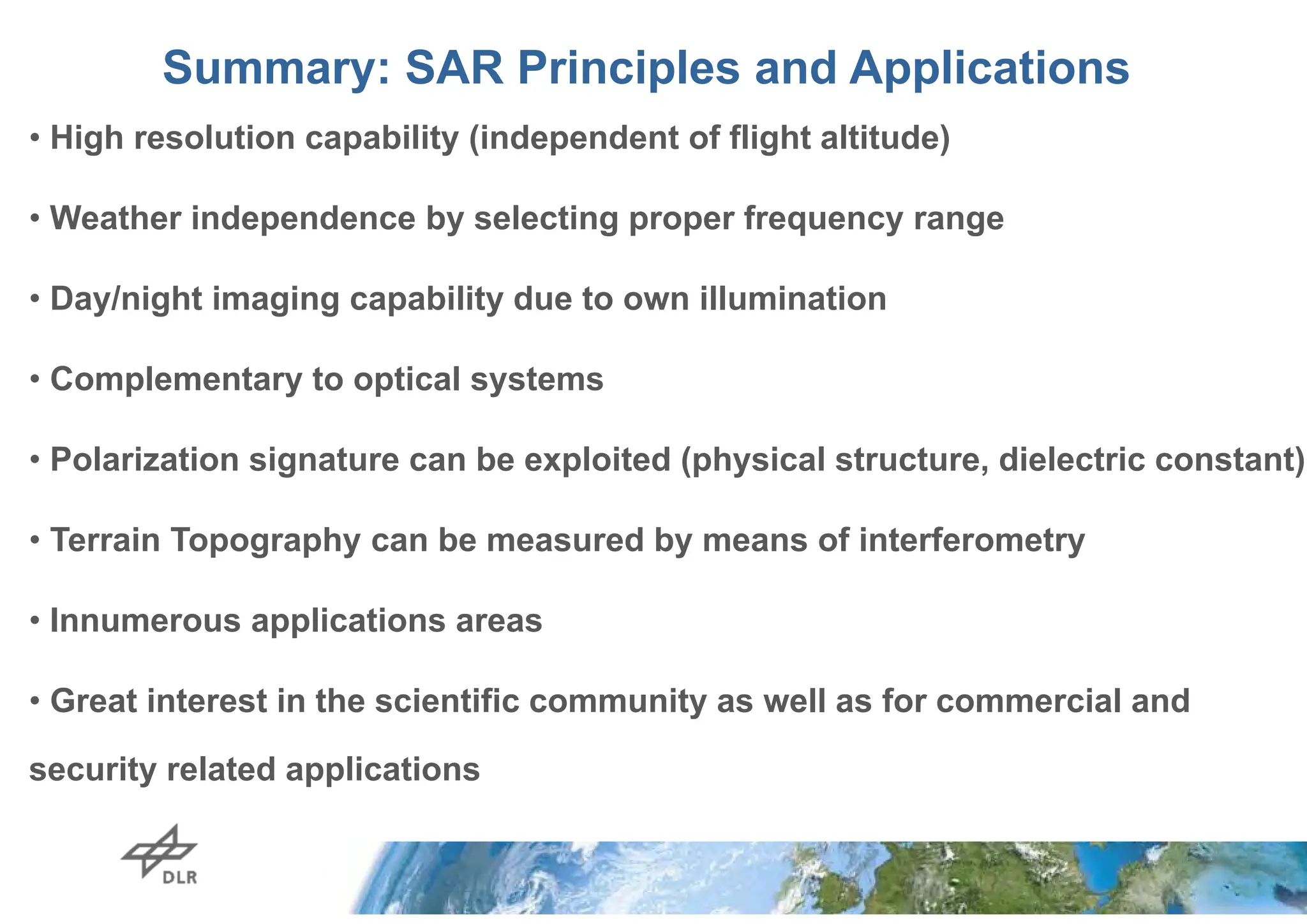
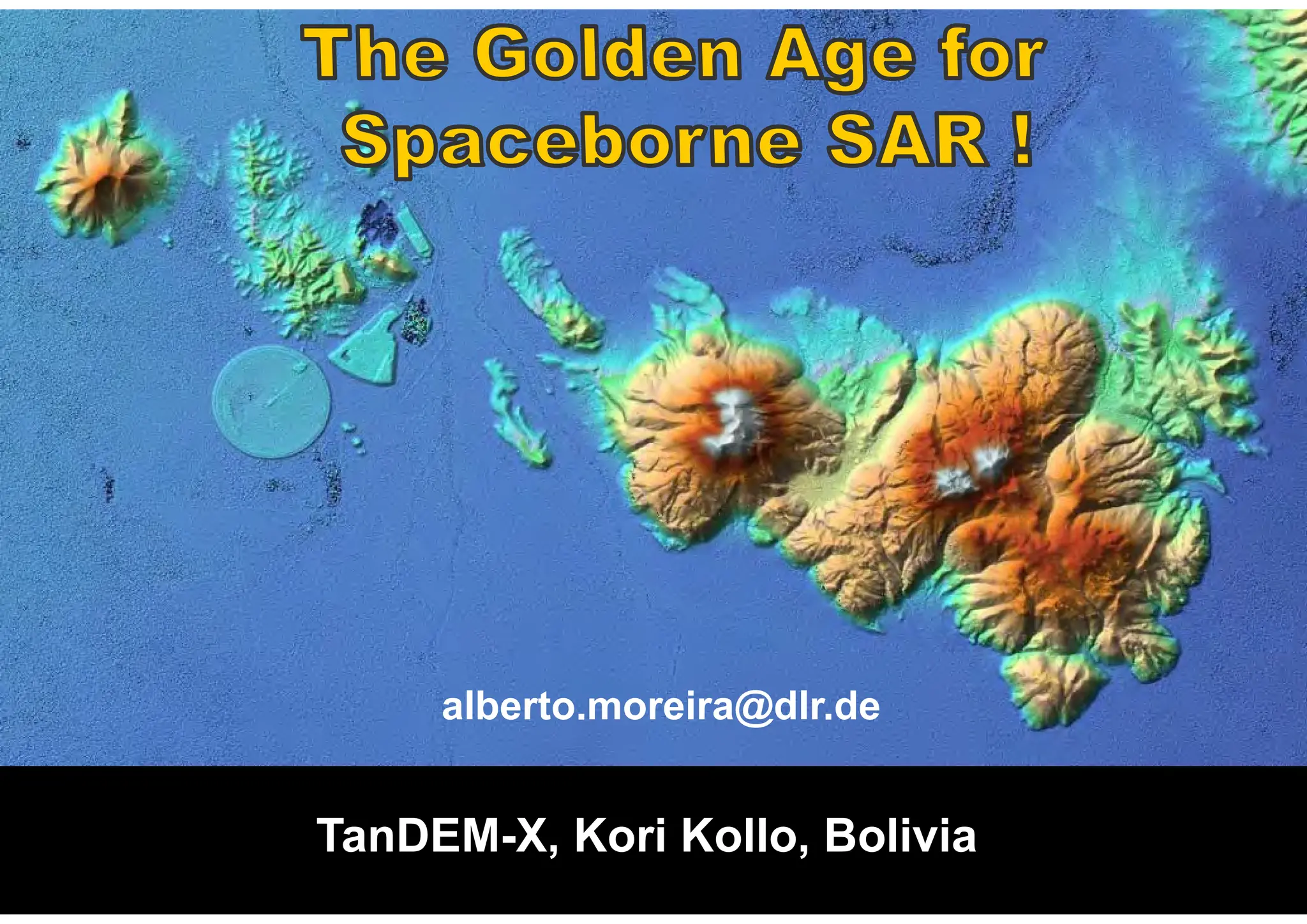
SAR Principles and Applications_SVKS.pdf

Marwan Younis
German Aerospace Center (DLR)
Microwaves and Radar Institute
82230 Oberpfaffenhofen, Germany
e‐mail: marwan.younis@dlr.de / Web: www.dlr.de/HR
Synthetic Aperture Radar (SAR):
Principles and Applications

German Aerospace Center Microwaves and Radar Institute
PART III
Theory: SAR Image Formation and
Image Properties

z
y
x
Antenna
Azimuth
range
SAR Basic Principle
1) pulsed radar system
(PRF = Pulse Repetition Frequency)
2) two dimensional imaging
(range x azimuth)
3) range resolution
4) azimuth resolution
5) Radar system must be coherent!
Te
Lsa
2
a
a
d


2
o
r
p
c
B



antenna
> 100 Mbit/s kbit/s
SAR Data Flow
Transmitter
Receiver
Data
Recording
Range
compression
Azimuth
compression
Image
evaluation
Image
interpretation
SAR
raw data
SAR
image data

signal generator
Mixer
power
amplifier
low noise
amplifier
circulator
base band signal
I
Q
A
D
A
D
-90°
I/Q demodulator
Synthetic Aperture Radar (SAR)
ultra stable
oscillator

Coherent Measurement Principle
transmit
t (time)
Total time delay 1 = 1
o
2 . r
c
Coherent demodulation
Received echo signal 1
phase change 1
1
4.
. object
phase r



  
1
4.
. object
phase r



  
1

A
Imaginary Part
Real Part

Coherent Measurement Principle
transmit
Total time delay 2 = 2
o
2 . r
c
Coherent demodulation
2
4.
. object
phase r



  
2
4.
. object
phase r



  
phase change 2
t (time)
Received echo signal 2
2

A
Imaginary Part
Real Part

   
 



 



 t
f
j
A
t
f
A 0
0 2
exp
2
cos
complex representation:
 


 j
A exp
after demodulation:

A
amplitude:
2
A
intensity, power:

phase:
Every pixel of a complex SAR image consists of a real and an imaginary part,
i.e. it is a phasor and contains amplitude and phase information.
A
Phasor Representation of SAR Signal
4.
. object
r



  
phase information
Imaginary Part
Real Part
o


amplitude information backscattering coefficient

r0
velocity
point target
range
/
fast
time
antenna beam
antenna
azimuth / slow time
pulse length
illumination time /
synthetic aperture length
2-D Raw Data Matrix
PRI
Number of Samples
for one point target:
1500 azimuth
30 000 range
Till = 0.5 s
Lsa = 3.6 km
 = 100 s @ 20% dc
V = 7 km/s
da = 5 m
a = 0.35°
@ 10 GHz
= 600 km

Formation of Azimuth Chirp Signal
time
azimuth
azimuth
signal
Number of Samples
for one point target:
1500 azimuth
30 000 range
time delay t=t1

Synthetic Aperture Formation and Processing
Detection
convolution
SAR
processor
point target response resolution of synthetic aperture
coherent summation
12
point target
flight
direction
beamwidth
of real aperture
antenna
SAR
sensor
Detection convolution
SAR
processor
received azimuth signal
point target response resolution of synthetic aperture
phase
corrections
coherent summation

Synthetic Aperture Radar (SAR)

SAR Processing (Image Formation)


raw data
SAR image
range compression
azimuth compression
range reference function
azimuth reference function

Pulse Compression by Convolution
convolution
t
e

e
T
point target response
range
reference
function
range
SAR signal
t
t

Linear Superposition of Chirps
convolution
t
t
t
range
reference
function
SAR signal
response of 3 point
targets

far range
near range
SAR Image
* *
azimuth
range
azimuth
range
raw data range compressed data
azimuth reference function
range reference function
amplitude
range
azimuth
amplitude

Summary: SAR Processing
1. Step: Range compression
• Generation of range reference function
• Matched filtering using convolution of range signal with range reference
function
2. Step: Azimuth compression
• Generation of azimuth reference function
• Matched filtering using convolution of azimuth signal with azimuth
reference function
3. Step: Calculation of the modulus of the SAR image (detection)
• This step is not required in case that the phase information is used (e.g.
polarimetry, interferometry etc.)
Normally the convolution is carried out in frequency domain

SAR Processing: 2D Matched Filter
he (x, r) ha (x, r) ui
2 + uq
2
azimuth
compression
detection
range
compression
SAR Processing
2D pulse
|uo (x, r)|
so (x, r)
impulse
response
function

• Examples of calibration targets with well-known reflectivity (Radar
Cross Section) for external calibration of the SAR system
Corner Reflector
Calibration Devices
Transponder

SAR Image of ASAR/ENVISAT, 12-10-02
D14
D01 D06
D02
D07
D03
D05
D11
D12
Munich
Alps
Strasbourg

SAR Image Properties
– Geometric Distortions –

27
Montserrat
Volcano
Stripmap
VV-pol.
• 9. Oct. 2007
Eruption: 29.
July 2008
• 1. Aug. 2008
• 12. Aug. 2008
near range
far range
azimuth
shadow
layover

Slant-to-Ground-Range Conversion
platform
(orbit)
height
ground range
á
á
´
a
• Slant range signal travel time
• Ground range projection onto a reference plane
Range Quantities

Geometric Distortion: Foreshortening
ground range
platform
(orbit)
height
Lground range
á
a
b
b́
• Slopes oriented to the radar appear compressed
Foreshortening

Geometric Distortion: Foreshortening
platform
(orbit)
height
ground range
Lground range
• Slopes oriented to the radar appear compressed
• Slopes tilted away from the radar appear lengthened
Foreshortening

Geometric Distortion: Layover
platform
(orbit)
height
ground range
a
b
á
b́
• an inversion in the image geometry!
Layover

Geometric Distortion: Shadow
ground range
platform
(orbit)
height
• Steep slopes oriented away from the radar return no
signal
Shadow

Consider the radar image below. What is the illumination direction of the radar?

range
azimuth near range
far range

range
azimuth
near range
far range

– Speckle –

Kaufbeuren, Germany
F-SAR, X-band quadpol
0.25m resolution

Kaufbeuren, Germany
F-SAR X-band quadpol
0.25m resolution
Speckle

• SAR image can be modeled as:
|u(x, r)| = |  (x, r)  uo (x, r) |
SAR signal modeling
where
|u(x, r)| SAR image
 (x, r) scene complex reflectivity
uo (x, r) SAR impulse response
Scene
 (x, r) se (x, r) sa (x, r)
he (x, r)
ha (x, r)
ui
2 + uq
2
azimuth
compression
azimuth
modulation
detection
pulse
modulation
pulse
compression
SAR processing
SAR image
|uo (x, r)|
• For a point target:  = 1
SAR system

SAR signal modeling
• Distributed targets have surface roughness comparable or smaller than
radar wavelength
• Resolution of the SAR sensor cannot resolve individual scatterers
• For each resolution cell,  (x, r) is equal to the sum of all scatterers contributions i. e.
|u(xo, ro)| = |  (xo, ro)  uo (x, r) | = |  i (xo, ro)  uo (x, r) |

random sum
real
imaginary

Szene mit Streuobjekten
Speckle
Im
Re
Im
Re
Radarbild (Betrag)
SAR image
imaged area with
distributed targets
random sum
random sum

Speckle
• Inherent to coherent systems
• Probability distribution function has a exponential distribution, i.e.
average value = standard deviation
• Speckle makes SAR image interpretation more difficult
E-SAR high resolution image
(0.6 m x 2 m)

Multi-Look Processing
antenna diagram
in azimuth direction
3 looks with 50% overlap
5 azimuth looks
 overlap of 50% between the looks
is commonly used.
azimuth
1 2 3 4 5 Look 1
Look 2
Look 3
azimuth

Σ
ui
2 + uq
2
sa (x, r)
ha3
(x, r)
ha2
(x, r)
ha1
(x, r)
ui
2 + uq
2
ui
2 + uq
2
• SAR impulse response function with multi-looking ( L looks):
• azimuth resolution deteriorates:
• Standard deviation of the speckle noise is reduced by the square root of the number of looks:
standard deviation = average value / sqrt( L)
 
2
2 1
,
( , ) 


L
i
i
ML
u x r
u x r
L
2
( , )
ML
u x r
2
1( , )
u x r
Multi-Look Processing (@ SAR Processor)
2
2 ( , )
u x r
2
3( , )
u x r
, .
 

a ML a L

Multi-Look Processing
image value image value image value
frequency
frequency
frequency

Statistics of SAR Signal for Distributed Targets
Scene
 (x)
Doppler
Modulation
Ba
f
Spectrum
ha1
(x)
ha2
(x)
ui
2 + uq
2
ui
2 + uq
2
ui
2 + uq
2
Gaussian
distribution
μi = μq= 0
 i=  q= P0 / 2
μi = μq= 0
 i=  q= P0 / 2
Exponential
distribution
μ = 2  i
2
 2
= μ2
Gamma
distribution
-distribution
μ = 2  i
2
2
= μ2
/ L0
Gaussian
distribution
μ ... average value ;  ... standard deviation
2
ML
u
ML
u

Multi-Look Processing (@ SAR Image)
• SAR impulse response function with average of L image pixels:
• azimuth resolution deteriorates:
• Standard deviation of the speckle noise is reduced by the square root of the number of looks:
standard deviation = average value / sqrt( L)
ui
2 + uq
2
Average
(boxcar
window)
sa (x, r)
ha(x, r)
2
( , )
ML
u x r
L = number of looks
, .
 

a ML a L
 
2
2 , 1
,
( , )
 



n m L
n m
n m
ML
u x r
u x r
L
2
( , )
u x r

5 looks
20 m x 20 m resolution
320 looks (average of 64 images)
20 m x 20 m ground resolution
Single-Look and Multi-Look Processing
ERS-1 satellite images (processing DLR-IMF)

original SAR image (1 look)
Airborne SAR AeS-1
speckle filtered
Adaptive Filtering
(Model based approach)
Speckle Reduction with Image Filtering

Summary: Speckle
• SAR image of distributed targets contains speckle noise.
• Speckle noise is inherent in coherent radar systems.
• The average value of the speckle amplitude is equal to its standard deviation
(exponential distribution).
• Multi-look processing or spatial averaging is used to reduce the speckle
noise. Standard deviation decreases with .
• An overlap of 50% between the looks is commonly used.
• Speckle noise can also be reduced by averaging the final image
eff
L

PART IV
Advanced SAR Techniques
and Future Developments

Advanced SAR Imaging Modes
- ScanSAR Mode -

ScanSAR Imaging
A
B
C
• Synthetic aperture is shared between the subswaths (not contiguous within one
subswath)
• Mosaic Operation is required in azimuth and range directions to join the azimuth
bursts and the range sub-swaths

ScanSAR Main Properties
• ScanSAR leads to a large swath width
•The azimuth signal consists of several bursts
• Azimuth resolution is limited by the burst duration
• Each target has a different frequency history depending on its azimuth location
Azimuth
azimuth frequency
Spectrum
A
B
C
C
A
B C

ScanSAR Imaging (Chickasha, Oklahoma, USA)
Subswath
2
Subswath
1
(near range)
Subswath
3
Subswath
4
(far range)
azimuth
SIR-C image
L-band, VV

ASAR SCANSAR Image (Munich Area) ASAR ScanSAR Image
ASAR Image

Comparison: ScanSAR vs. Stripmap (TerraSAR-X)
ScanSAR (HH)
150 MHz
17 m resolution
1 (az) x 6.9 (rg) looks
ascending orbit
Stripmap (HH)
150 MHz
7 m resolution
2.9 (az) x 3.4 (rg) looks
descending orbit
3 days time separation

ScanSAR
EEC-RE
17 m res.
illumination
~3 km x 4 km
ScanSAR

Stripmap
EEC-RE
7 m res.
illumination
~3 km x 4 km
Stripmap

TOPS-SAR (Terrain Observation by Progressive Scan)
ScanSAR
Shares illumination time between
multiple swaths
TOPS-SAR
Shares illumination time between
multiple swaths
Improved image quality

Advanced SAR Imaging Modes
- Spotlight Mode -

Azimuth
Spotlight Synthetic Aperture
End of
imaging
Begin of
imaging
image center
synthetic aperture of
stripmap mode
• Non continuous imaging mode, but very high azimuth resolution
• Spotlight azimuth resolution
Spotlight SAR Imaging

Stripmap image
3 m azimuth resolution
Spotlight image
0.46 m azimuth resolution
E-SAR System, X-Band, Oberpfaffenhofen, Germany
Spotlight SAR Imaging

High Resolution Spotlight, HH-Pol., spot_040, 37° inc. angle, 150 MHz
Chuquicamata, Chile
L1B SAR Processing: High Resolution Spotlight
HR Spotlight (VV), 150 MHz range bandwidth, θincid ≈ 35°, 5 km x 10 km
az
rng
Chuquicamata, Chile

Folie 67 Pau.Prats@dlr.de
Oberpfaffehofen
Spotlight Imaging Mode

SAR Application Trends
Trends in Earth Science & Applications:
 Day / night, all-weather coverage of the Earth‘s surface
 Frequent revisit times (time series):
 hours to 1 day: coastal zones, ocean, traffic and disaster monitoring
 days to weeks: differential interferometry, soil moisture, agricultural areas
 months to year: tropical, temperate and boreal forests, differential interf.
 Variable resolution (1 to 100 m) and wide coverage (25 to 450 km swath width)
 High (2 m) and medium resolution (10-15 m) global topography
 Information products of key inputs to global change models:
 above ground biomass, soil moisture, wetland areas, land cover types
 ocean surface & currents, ice mass balance, glacier velocity
 Calibrated and geo-coded data products are required (e.g. compatibility to GIS)
 Model based inversion algorithms are needed for reliable information extraction

German Aerospace Center Microwaves and Radar Institute
Summary: SAR Principles and Applications
• High resolution capability (independent of flight altitude)
• Weather independence by selecting proper frequency range
• Day/night imaging capability due to own illumination
• Complementary to optical systems
• Polarization signature can be exploited (physical structure, dielectric constant)
• Terrain Topography can be measured by means of interferometry
• Innumerous applications areas
• Great interest in the scientific community as well as for commercial and
security related applications

References I
SAR Principles and Applications
 CEOS EO Handbook – Catalogue of Satellite Instruments. On-line available: http://www.eohandbook.com, Oct. 2012.
 Curlander, J.C., McDonough, R.N.: Synthetic Aperture Radar: Systems and Signal Processing. Wiley, 1991.
 Elachi, C. and J. van Zyl, Introduction to the Physics and Techniques of Remote Sensing. John Wiley & Sons, 2006
 Henderson, F. und Lewis, A.: Manual of Remote Sensing: Principles and Applications of Imaging Radar. Wiley, 1998.
 Lee, J.S. and Pottier, E.: Polarimetric Radar Imaging: From Basics to Applications. CRC Press, 2009.
 Massonnet, D. and Souryis, J.C.: Imaging with Synthetic Aperture Radar. EPFL & CRC Press, 2008.
 McDonough, R.N. et al: Image Formation from Spaceborne Synthetic Aperture Radar Signals. Johns Hopkins APL
Technical Digest, Vol. 6, No. 4, 1985, S. 300-312.
 Moreira, A., Prats-Iraola, P., Younis, M., Krieger, G., Hajnsek, Irena and Papathanassiou, K.: A Tutorial on Synthetic
Aperture Radar. IEEE Geoscience and Remote Sensing Magazine, 1 (1), 2013, pp. 6-43.
 Tomiyasu, K.: Tutorial Review of Synthetic-Aperture Radar (SAR) with Applications to Imaging of the Ocean Surface.
In: IEEE Proc., Vol. 66, No. 5, May 1978.
 Woodhouse, I.: Introduction to Microwave Remote Sensing, CRC, Taylor & Francis, 2006.

References II
SAR Processing
 Cumming, Ian and Frank Wong, Digital Processing of Synthetic Aperture Radar Data, Artech House, 2005
 Franceschetti G. und R. Lanari.: Synthetic Aperture Radar Processing. CRC Press, USA, 1999
 Li, F.K., Croft, C., Held,D.: Comparison of Several Techniques to Obtain Multiple-Look SAR Imagery. In: IEEE
Trans. Geoscience and Remote Sensing, Vol. 21, No. 3, Juli 1983.
 Moreira, A., Mittermayer, J., Scheiber, R.: Extended Chirp Scaling Algorithm for Air- and Spaceborne SAR Data
Processing in Stripmap and ScanSAR Imaging Modes. In: IEEE Trans. Geoscience and Remote Sensing, Vol. 34,
No. 5, 1996.
 Oliver, C. und S. Quegan. Understanding Synthetic Aperture Radar Images. SciTech Publishing, Inc., 2004.
 Raney, R. K.: Theory and Measure of Certain Image Norms in SAR. IEEE Trans. Geosci. Remote Sensing, Vol. 23,
No.3, Mai 1985.
 Raney, R. K. und Wessels, G. J.: Spatial Considerations in SAR Speckle Simulation. IEEE Trans. Geosci. Remote
Sensing, Vol. 26, No. 5, Sept. 1988, S. 666-672.
 Tomiyasu, K.: Conceptual Performance of a Satellite Borne, Wide Swath Synthetic Aperture Radar. In: IEEE Trans.
Geoscience and Remote Sensing, Vol. 19, No. 2, April 1981, S. 108-116.

TanDEM-X, Kori Kollo, Bolivia
alberto.moreira@dlr.de

SAR Principles and Applications_SVKS.pdf

More Related Content

Similar to SAR Principles and Applications_SVKS.pdf

Recently uploaded

SAR Principles and Applications_SVKS.pdf