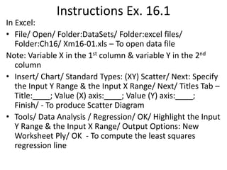
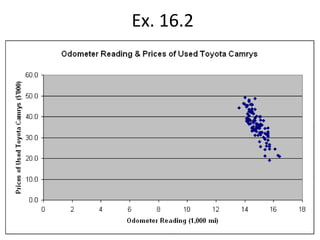
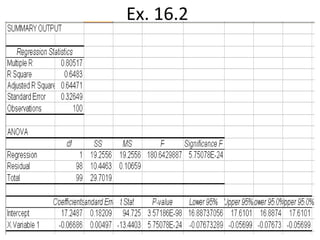
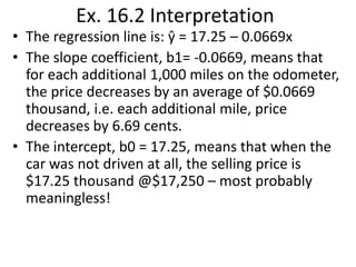
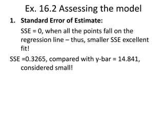
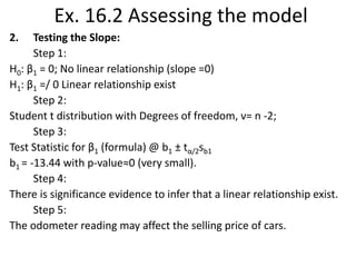
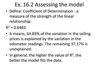
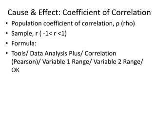
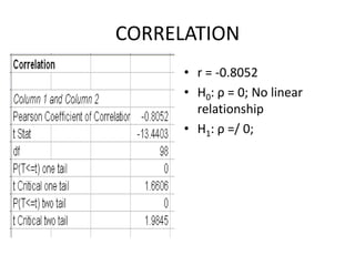
The document provides instructions for using Excel to analyze the relationship between two variables, the odometer reading (X) and selling price (Y) of used cars. It describes how to produce a scatter plot and regression line to model the relationship, and how to interpret the results including the slope, intercept, standard error, coefficient of determination (R2), and testing whether there is a significant linear relationship between the variables.

2. Instructions Ex. 16.1
In Excel:
• File/ Open/ Folder:DataSets/ Folder:excel files/
Folder:Ch16/ Xm16-01.xls – To open data file
Note: Variable X in the 1st column & variable Y in the 2nd
column
• Insert/ Chart/ Standard Types: (XY) Scatter/ Next: Specify
the Input Y Range & the Input X Range/ Next/ Titles Tab –
Title:____; Value (X) axis:____; Value (Y) axis:____;
Finish/ - To produce Scatter Diagram
• Tools/ Data Analysis / Regression/ OK/ Highlight the Input
Y Range & the Input X Range/ Output Options: New
Worksheet Ply/ OK - To compute the least squares
regression line

3. Ex. 16.2

4. Ex. 16.2

5. Ex. 16.2 Interpretation
• The regression line is: ŷ = 17.25 – 0.0669x
• The slope coefficient, b1= -0.0669, means that
for each additional 1,000 miles on the odometer,
the price decreases by an average of $0.0669
thousand, i.e. each additional mile, price
decreases by 6.69 cents.
• The intercept, b0 = 17.25, means that when the
car was not driven at all, the selling price is
$17.25 thousand @$17,250 – most probably
meaningless!

6. Ex. 16.2 Assessing the model
1. Standard Error of Estimate:
SSE = 0, when all the points fall on the
regression line – thus, smaller SSE excellent
fit!
SSE =0.3265, compared with y-bar = 14.841,
considered small!

7. Ex. 16.2 Assessing the model
2.
Testing the Slope:
Step 1:
H0: β1 = 0; No linear relationship (slope =0)
H1: β1 =/ 0 Linear relationship exist
Step 2:
Student t distribution with Degrees of freedom, ν= n -2;
Step 3:
Test Statistic for β1 (formula) @ b1 ± tα/2sb1
b1 = -13.44 with p-value≈0 (very small).
Step 4:
There is significance evidence to infer that a linear relationship exist.
Step 5:
The odometer reading may affect the selling price of cars.

8. Ex. 16.2 Assessing the model
• Define: Coefficient of Determination - a
measure of the strength of the linear
relationship:
R2 = 0.6483
• It means, 64.83% of the variation in the selling
prices is explained by the variation in the
odometer readings. The remaining 37.17% is
unexplained.
• In general, the higher the value of R2, the
better the model fits the data.

9. Cause & Effect: Coefficient of Correlation
•
•
•
•
Population coefficient of correlation, ρ (rho)
Sample, r ( -1< r <1)
Formula:
Tools/ Data Analysis Plus/ Correlation
(Pearson)/ Variable 1 Range/ Variable 2 Range/
OK

10. CORRELATION
• r = -0.8052
• H0: ρ = 0; No linear
relationship
• H1: ρ =/ 0;

12. Data source: Managerial
Statistics, 9th Ed. (Keller)
CENGAGE