This document is the master's thesis of Yiting Wu titled "Development and Implementation of a Control System for a quadrotor UAV". The thesis describes the development and testing of control systems for a quadrotor drone. It includes the construction of a test platform with an inertial measurement unit and microcontroller. Three control algorithms - nonlinear feedback linearization, simple PD control, and PD control with partial differentiation - are designed, simulated, implemented on the test platform, and evaluated. The best performing control algorithm is determined based on simulation and implementation results.


![5 Attitude Control Algorithm Design .................................................... 41
5.1 Nonlinear Control using Feedback-Linearization[1] .................................... 43
5.1.1 Control Algorithm Design .................................................................... 43
5.1.2 Control Algorithm Implementation ..................................................... 46
5.2 Simple PD Controller .................................................................................. 47
5.2.1 Controller Algorithm Design ................................................................ 47
5.2.2 Controller Algorithm Implementation ................................................ 49
5.3 PD controller Design with Partial Differential ............................................ 50
5.3.1 Controller Algorithm Implementation ................................................ 50
5.3.2 Controller Algorithm Implementation ................................................ 52
5.4 Motor Torque Design ................................................................................. 53
6 Simulation and Implementation Results .......................................... 55
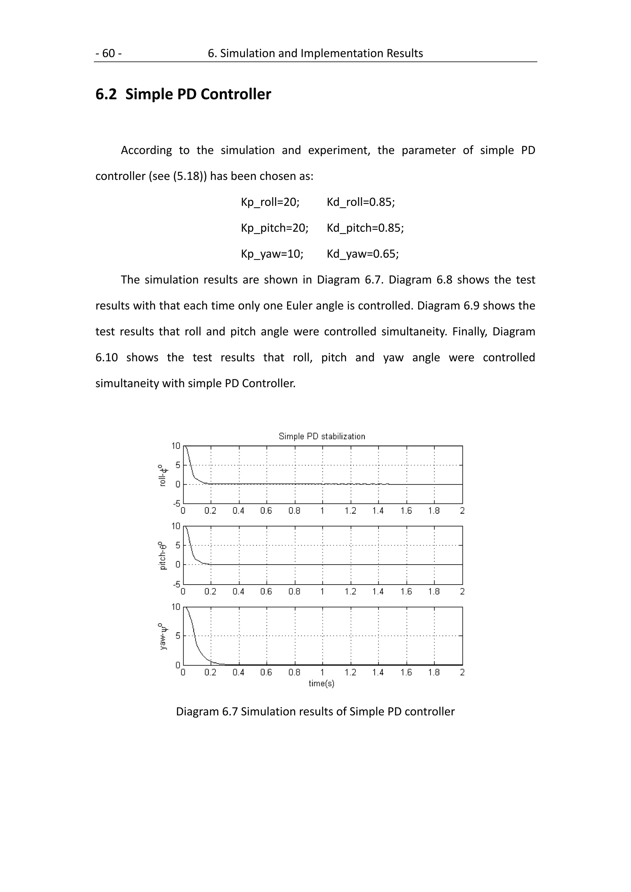
6.1 Nonlinear Feedback Control....................................................................... 56
6.2 Simple PD Controller .................................................................................. 60
6.3 PD Controller with partial differential ........................................................ 63
7 Conclusion .................................................................................................. 67
7.1 Comparison of the control algorithms ....................................................... 67
7.2 Project Contributions ................................................................................. 69
7.3 Future Work................................................................................................ 70
List of Figures ....................................................................................................... 73
List of Diagrams.................................................................................................... 75
List of Tables ........................................................................................................ 76
Appendix .............................................................................................................. 76
Bibliography ......................................................................................................... 77](https://image.slidesharecdn.com/2009developmentandimplementationofacontrolsystemforaquadrotoruav-111213204238-phpapp02/75/2009-development-and-implementation-of-a-control-system-for-a-quadrotor-uav-10-2048.jpg)
![1. Introduction -3-
(IMU) sensor equipped on quadrotor. There are some contributions in the literature
that are concerned with control system design for quadrotor vehicles. Many of the
proposed control systems are based on a linearized model and conventional PID- or
state space control [5], [11], [15]while the other approaches apply SDRE or Nonlinear
Feedback control [1] , [18]. In this paper the Nonlinear Feedback control [18] is studied
and chosen to implement on the real quadrotor. In order to compare Nonlinear
Feedback control with the conventional PID control technique, a PID controller is
designed and implemented on the quadrotor. Finally according to the simulation and
test results, the features of these two kinds of control techniques are summarized.
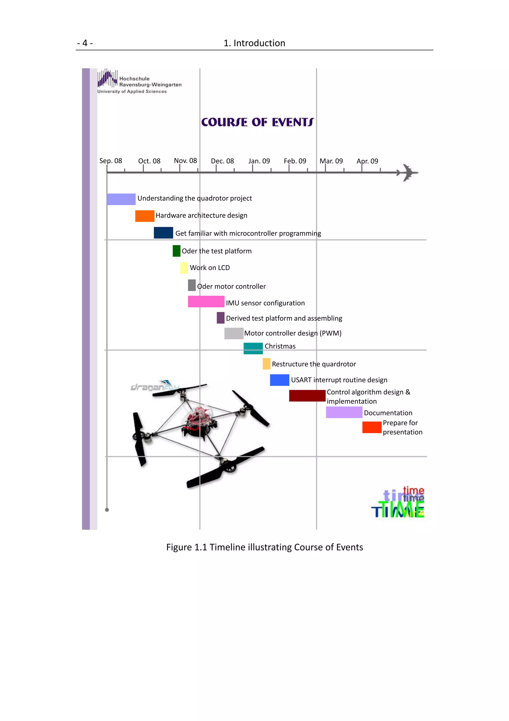
1.2 Course of events
This section will briefly give insight into the intermediate goals and objectives on
the way towards achieving autonomous hovering flight. Figure 1.1 provides an
overview of the course of events during the whole thesis period.
At the beginning of September work started from reading the corresponding
literatures to provide a basic understanding of how the quadrotor operates, what
kind of physics are involved and essentially how to combine this knowledge into a
useful model for control purpose. The bold goal at that time was to be able to hover
at the end of the thesis. After that, a lot of time and efforts were put on get related
electronic unit ready to work, including the IMU configuration, motor controller
design, USART interrupt routine design and so on. At the end, two controllers were
implemented on the quadrotor and could control the attitude with small tolerances.](https://image.slidesharecdn.com/2009developmentandimplementationofacontrolsystemforaquadrotoruav-111213204238-phpapp02/75/2009-development-and-implementation-of-a-control-system-for-a-quadrotor-uav-13-2048.jpg)

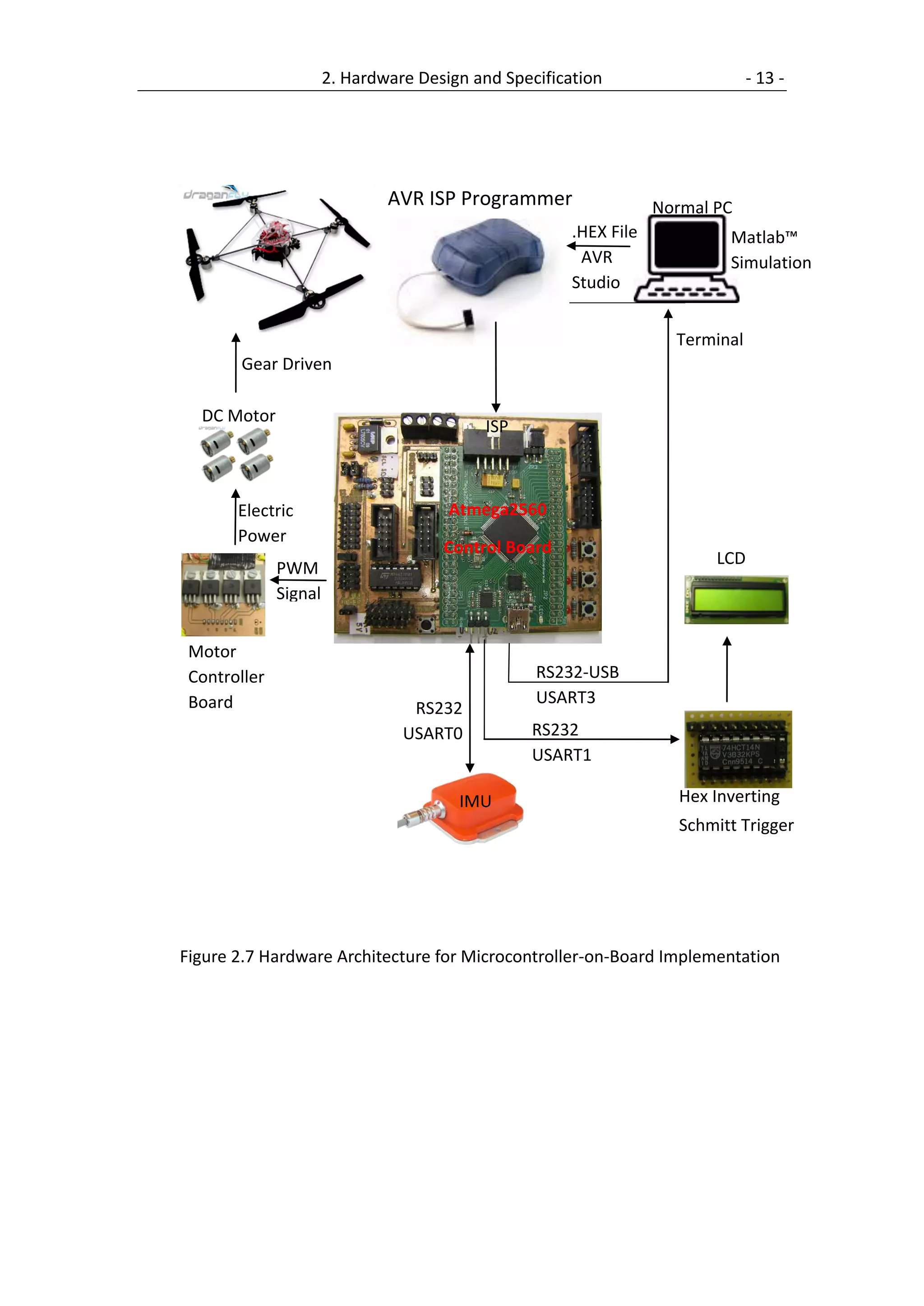
![-8- 2. Hardware Design and Specification
2.1.1 Real-Time Implementation
A system is a real-time system when it can support the execution of applications
with time constraints on that execution. Real-time control is a popular term for a
certain class of digital controllers. For effective digital control, it is critical that sample
time be constant. Real-time control achieves nearly constant sample time. The most
used real time application tools are Matlab Real-Time Workshop™ or xPC Target™. By
using these tools you can create a real-time application to let the system run while
synchronized to a real-time clock. This allows the system to control or interact with
an external system. Figure 2.1 shows the hardware architecture for the real-time
control concept which is developed by student group from AALBORG University as
their master thesis.[5]
As the Figure 2.1 shows it has been chosen to equip the quadrotor with sensors
as GPS for absolute position estimate, Magnetometer for information about heading
range finder to aid the GPS in getting an altitude estimate, IMU for the possibility to
propagate position and attitude. Besides all these sensors there are a number of
components related to manual flight and other safety feature. All together these
transducers are connected to the main CPU, some via a slave processor, the Robostix
board, which is built up around a 16 MHz Atemega128 processor. The Gumstix
features a 400 MHz Intel XScale processor of the type PXA255. It has 16 MB flash
memory and 64 MB of SDRAM. The embedded Linux system is running on this
Gumstix. Wifistix is a fully configurable wireless board, following the 802.11(g)
standard, which means that the bandwidth can be up to 54 Mb/s.](https://image.slidesharecdn.com/2009developmentandimplementationofacontrolsystemforaquadrotoruav-111213204238-phpapp02/75/2009-development-and-implementation-of-a-control-system-for-a-quadrotor-uav-18-2048.jpg)
![2. Hardware Design and Specification -9-
Figure 2.1 Hardware Architecture for real-time application [5]
Figure 2.2 Robostix Board Figure 2.3 Gumstix Figure 2.4 Wifistix](https://image.slidesharecdn.com/2009developmentandimplementationofacontrolsystemforaquadrotoruav-111213204238-phpapp02/75/2009-development-and-implementation-of-a-control-system-for-a-quadrotor-uav-19-2048.jpg)
![- 10 - 2. Hardware Design and Specification
First the Robostix is treated which has the main task of forwarding sensor data
to the Gumstix. The low level code is written in C and cross compiled to generate a
hex file which is loaded onto the Atmega128. Second the Gumstix software is treated
which is written in high level C code. This software is also cross compiled to fit the
system specific architecture of the Gumstix, namely the Intel Xscale PXA255
processor. Next the Development Host Machine software is described which is
basically defined by a Linux Soft Real Time Target application in Matlab™/Simlink™. It
is in this environment the controller will be derived and also implemented.[5] The
interaction between the components and the main process is illustrated in Figure
2.5.
Figure 2.5 The main process interacting with peripheral components [5]](https://image.slidesharecdn.com/2009developmentandimplementationofacontrolsystemforaquadrotoruav-111213204238-phpapp02/75/2009-development-and-implementation-of-a-control-system-for-a-quadrotor-uav-20-2048.jpg)
![- 16 - 2. Hardware Design and Specification
2.4 IMU
IMU stands for inertial measurement unit. The IMU sensor MTi which is used in
this project is produced by Xsens™, more detailed product information can be found
on www.xsens.com. The MTi is a miniature, gyro-enhanced Attitude and Heading
Reference System (AHRS). Its internal low-power signal processor provides drift-free
3D orientation as well as calibrated 3D acceleration, 3D rate of turn (rate gyro) and
3D earth-magnetic field data. The MTi is an excellent measurement unit for
stabilization and control of cameras, robots, vehicles and other equipment. Figure
2.10 shows the overview of the MTi sensor.
Figure 2.10 MTi Overview
2.4.1 Sensor Communication Features
Interface through COM-object API, capable to access the MTi directly in
application software such as MATLAB™, LabVIEW™, Excel (Visual Basic).
→Please refer to the MT Software Development Kit Documentation[6] for
more information on this topic.](https://image.slidesharecdn.com/2009developmentandimplementationofacontrolsystemforaquadrotoruav-111213204238-phpapp02/75/2009-development-and-implementation-of-a-control-system-for-a-quadrotor-uav-26-2048.jpg)
![2. Hardware Design and Specification - 17 -
Direct low-level communication with MTi (RS-232/422).
→Please refer to the MTi and MTx Low-level communication protocol
Documentation[6] for more information on this topic.
2.4.2 Co-ordinate systems
All calibrated sensor readings (accelerations, rate of turn, earth magnetic field)
are in the right handed Cartesian co-ordinate system as defined in Figure 2.11 (a).
This co-ordinate system is body-fixed to the quadrotor and is defined as the sensor
co-ordinate system.
(a) (b)
Figure 2.11 MTi with sensor-fixed co-ordinate system overlaid
A positive rotation is always „right-handed“, i.e. defined according to the right
hand rule (corkscrew rule). This means a positive rotation is defined as clockwise in
the direction of the axis of rotation, Figure 2.11 (b).](https://image.slidesharecdn.com/2009developmentandimplementationofacontrolsystemforaquadrotoruav-111213204238-phpapp02/75/2009-development-and-implementation-of-a-control-system-for-a-quadrotor-uav-27-2048.jpg)
![- 18 - 2. Hardware Design and Specification
2.4.3 Output Modes
Quaternion orientation output mode
Euler angles orientation output mode
Rotation Matrix orientation output mode
Calibrated data output mode
→Please refer to the MTi and MTx User Manual[6] for more information on
this topic.](https://image.slidesharecdn.com/2009developmentandimplementationofacontrolsystemforaquadrotoruav-111213204238-phpapp02/75/2009-development-and-implementation-of-a-control-system-for-a-quadrotor-uav-28-2048.jpg)
![2. Hardware Design and Specification - 19 -
2.5 Microcontroller Board
The original electronic circuit board (Figure 2.12 (a)) of the commercial
DraganFlyer is equipped with Radio Frequency (RF) control module, three Piezo
electric gyro sensors in X, Y and Z direction which are used for stabilization, four
infrared sensors which are used for thermal intelligence to maintain the altitude.
→Please refer to the df5ti-manual[6] for more information on this topic.
(a) (b)
Figure 2.12 Electronic circuit board
Since there is no interface between the microcontroller and PC, the
microcontroller cannot be programmed by ourselves. So it is necessary to remove
the original board and develop our own one. Thanks to Martin Binswanger who has
developed one board for his bachelor project, this board is also competent for my
quadrotor project. Thus my quadrotor project is based on Martin’s electronic board.
The board is shown in Figure 2.12 (b).](https://image.slidesharecdn.com/2009developmentandimplementationofacontrolsystemforaquadrotoruav-111213204238-phpapp02/75/2009-development-and-implementation-of-a-control-system-for-a-quadrotor-uav-29-2048.jpg)
![- 20 - 2. Hardware Design and Specification
2.6 Motor Controller
The functions of the motor controller are that, a). give the power supply to the
motors; b). amplify the motor speed control signal, here is PWM signal. Since the
motor controller give the power supply to the motor, so the maximal load current
should be taken into account. As from the measurement result, when the rotor
rotates on full speed, the current in the wire is 2.5 A, so the maximal load current of
the motor controller for each motor should bigger than 2.5 A. After searching on the
market, finally the motor controller BTS 621 L1 from Siemens[10] has been chosen,
whose maximal Load current (each) is 4.4 A. Then the motor controller board has
been made with four motor controllers, where one controller controls only one
motor. Figure 2.13 shows the motor controller board.
Figure 2.13 Motor controller Board](https://image.slidesharecdn.com/2009developmentandimplementationofacontrolsystemforaquadrotoruav-111213204238-phpapp02/75/2009-development-and-implementation-of-a-control-system-for-a-quadrotor-uav-30-2048.jpg)
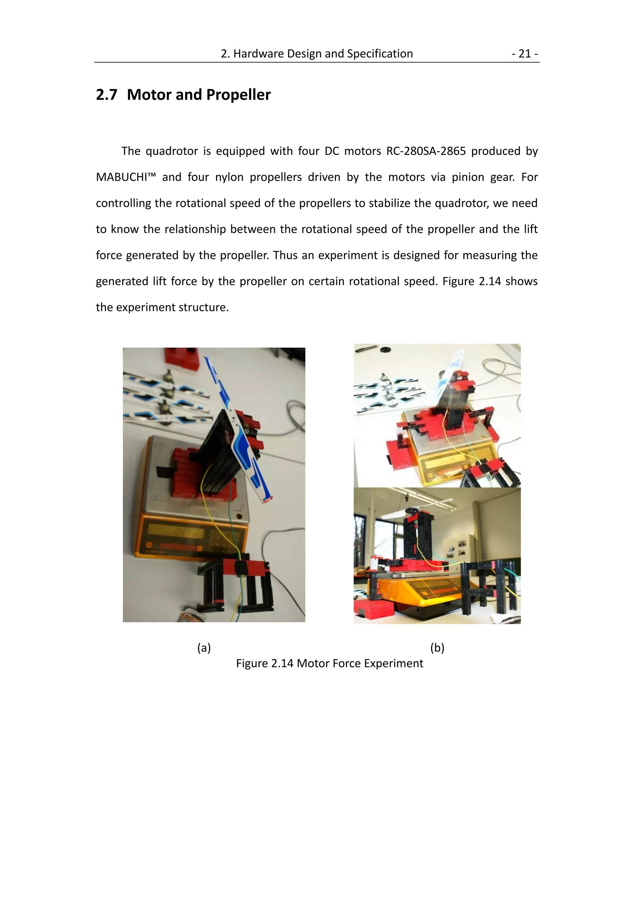
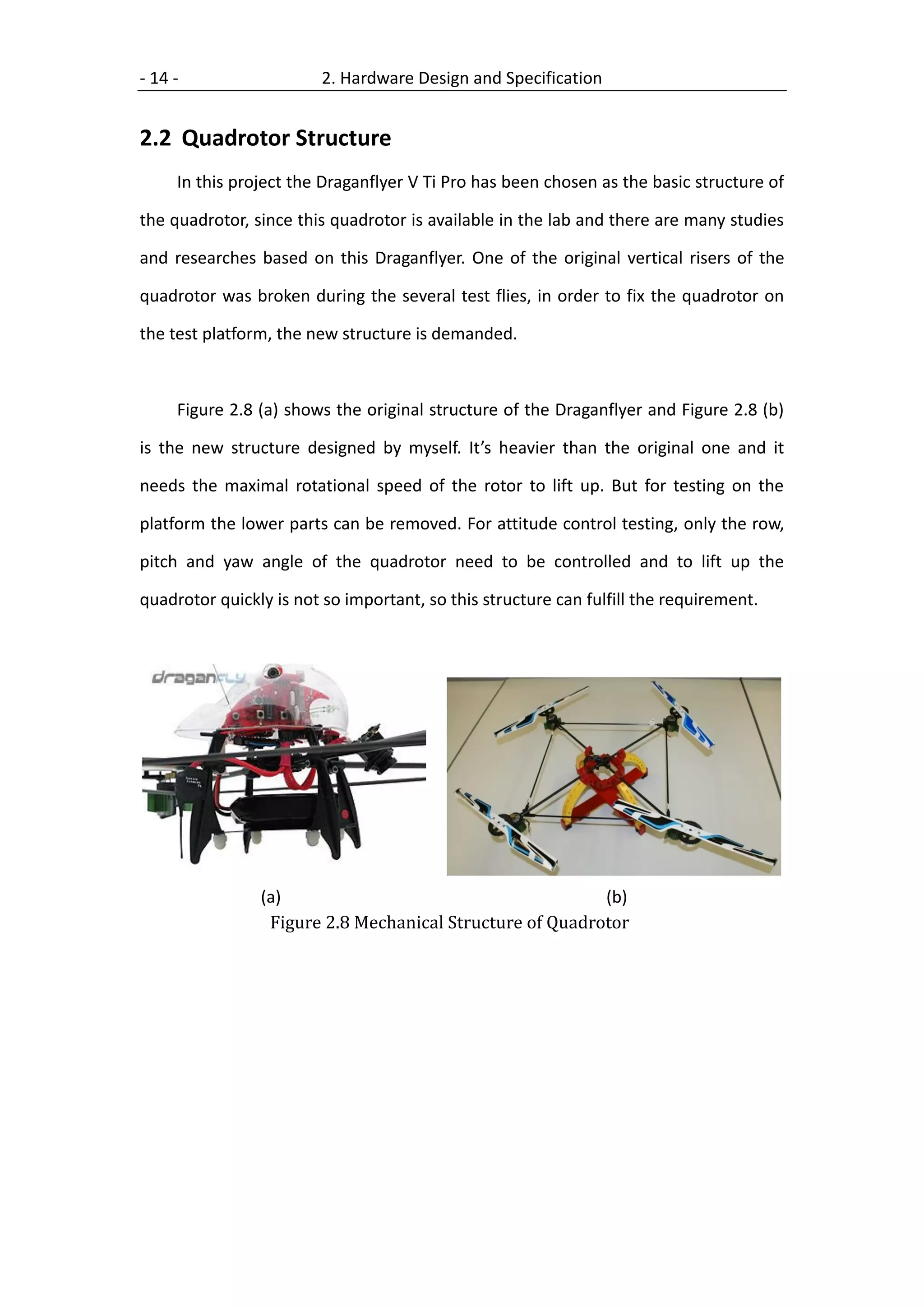
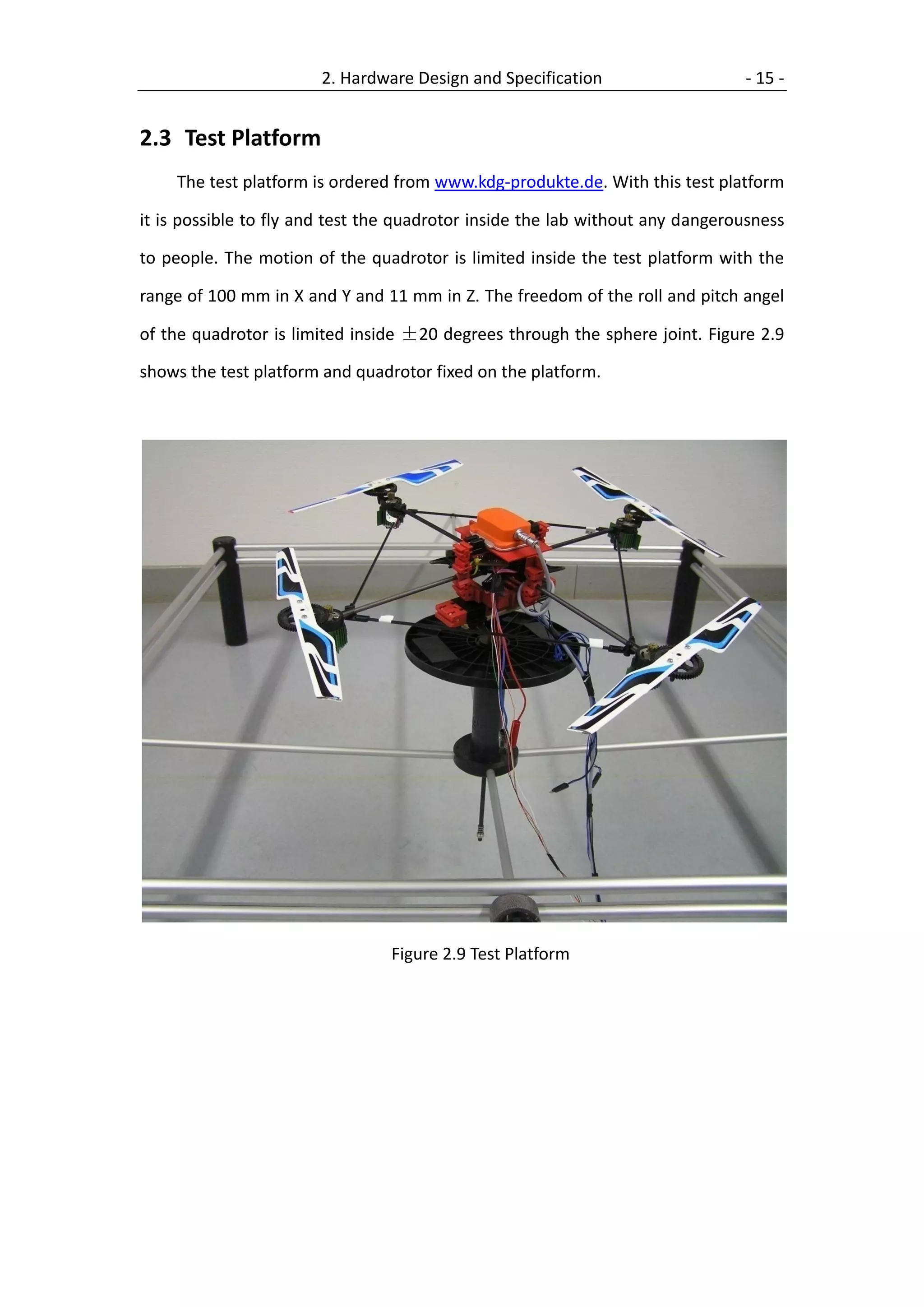
![- 24 - 2. Hardware Design and Specification
2.8 Identification of the constants
To identify the constants of the quadrotor, there are different approaches to
estimate a constant. The experiments to determine the constants are described in
[11]. Since we use the same quadrotor mode (Figure 2.6) with the mode used in
paper [11], so the parameters determined in [11] can be used here too. Table 2.2
gives the quadrotor constants.
Table 2.2 quadrotor constants
Parameter Value Unit Remark
9.81 / 2 gravity
0.55 Mass of the quadrotor
0.21 Length of the lever
= 3 2 Inertias around and axis
4.85 ∙ 10 ∙
8.81 ∙ 103 ∙ 2 Inertia around axis
4.85 ∙ 103 ∙ 2 Rotor Inertia
−6 2
2.92 ∙ 10 ∙ Thrust factor
−7 2
1.12 ∙ 10 ∙ Drag factor
1 0.309 N Thrust factor, Front Motor 1
1 0.345 N Thrust factor, Back Motor 2
1 0.25 N Thrust factor Left Motor 3
1 0.34 N Thrust factor, Right Motor 4
1 0.0063 N Thrust factor, Front Motor 1
2 0.0053 N Thrust factor, Back Motor 2
3 0.006 N Thrust factor, Left Motor 3
4 0.005 N Thrust factor, Right Motor 4](https://image.slidesharecdn.com/2009developmentandimplementationofacontrolsystemforaquadrotoruav-111213204238-phpapp02/75/2009-development-and-implementation-of-a-control-system-for-a-quadrotor-uav-34-2048.jpg)
![- 26 - 3. Software Preparation and Specification
The checksum value of the message can be calculated by the following
equation.
= ( + + + ) + 1 (3.1)
For example, we have the message of set output mode:
PREAMBLE BID MID LEN DATA1 DATA2 CHECKSUM
0xFA 0xFF 0xD0 0x02 0x00 0x06 0x29
For example:
SUM=0xFF+0xD0+0x02+0x00+0x06=0x1D7=111010111(binary)
complement (SUM)=000101000
CHECKSUM=complement+1=101001(binary)=0x29
First of all, the initialization of the IMU was executed with a power-cycle or reset
of the microcontroller. Through the initialization of the IMU (subprogram:
imu_init(…)[12]) the properties of the data output are configured.
Baudrate 115k2
Sampling Rate 100Hz
Output Rate 100Hz
Output Mode Calibrated data--rate of turn and Euler angles
Table 3.2 The used configuration of IMU
After the initialization the IMU goes from Configuration State to the
Measurement State. The IMU sends 100 data packets pro second through RS232
interface to the microcontroller. Every data packet has the size of 29 Bytes.](https://image.slidesharecdn.com/2009developmentandimplementationofacontrolsystemforaquadrotoruav-111213204238-phpapp02/75/2009-development-and-implementation-of-a-control-system-for-a-quadrotor-uav-36-2048.jpg)
![3. Software Preparation and Specification - 27 -
The measured data of rate of turn and Euler angles are coded in float number
which is 4 Bytes long. The received Bytes are checked first and then stored in one
Bufferarray(MH_rx_buffer[32])[12]. In Bufferarry the data are found again under
following index n:
n Data
0 Preamble
1 BID
2 MID
3 Length
4 to 7 4 Byte Float Number = Rate of turn around X-Axis
8 to 11 4 Byte Float Number = Rate of turn around Y-Axis
12 to 15 4 Byte Float Number = Rate of turn around Z-Axis
16 to 19 4 Byte Float Number = Euler Angle around X-Axis
20 to 23 4 Byte Float Number = Euler Angle around Y-Axis
24 to 27 4 Byte Float Number = Euler Angle around Z-Axis
Table 3.3 The Bufferarray for the IMU Data
In order to make the four single elements(each one is 1 byte) of the Bufferarrays
as one float number for the software which is 4 bytes, the subprogram “float
make_float(…)”[12] must be used.](https://image.slidesharecdn.com/2009developmentandimplementationofacontrolsystemforaquadrotoruav-111213204238-phpapp02/75/2009-development-and-implementation-of-a-control-system-for-a-quadrotor-uav-37-2048.jpg)
![- 28 - 3. Software Preparation and Specification
3.1.2 Message usage in “imu_init()”
IMU-Reset:
{0xfa, 0xff, 0x40, 0x00, 0xC1};
IMU-WakeUp:
{0xfa, 0xff, 0x3f, 0x00, 0xC2};
SetBaudrate: 115k2
{0xfa,0xff,0x18,0x01,0x02,0xE6 };
ReqBaudrate:
{0xfa,0xff,0x18,0x00,0xE9};
SetPeriod: sets 10 ms to the sampling period of the device used in Measurement
State
{0xfa,0xff,0x04,0x02,0x04,0x80,0x77};
SetSkipFactor: every MTData message is sent
{0xfa,0xff,0xD4,0x02,0x00,0x00,0x2B};
SetOutputMode: calibrated data output
{0xfa,0xff,0xD0,0x02,0x00,0x06,0x29};
SetOutputsettings: rate of turn and Euler angle enable, acceleration and
magnetometer disable
{0xfa,0xff,0xD2,0x04,0x00,0x00,0x00,0x54,0xD7};
SetExtOutputMode: Analog Output Mode disable
{0xfa,0xff,0x86,0x02,0x00,0x00,0x79};
GotoMeasurement: enter the Measurement State
{0xfa,0xff,0x10,0x00,0xF1};
→ Please refer to the MTi and MTx Low-level Communication[6] for more
information on this topic.](https://image.slidesharecdn.com/2009developmentandimplementationofacontrolsystemforaquadrotoruav-111213204238-phpapp02/75/2009-development-and-implementation-of-a-control-system-for-a-quadrotor-uav-38-2048.jpg)
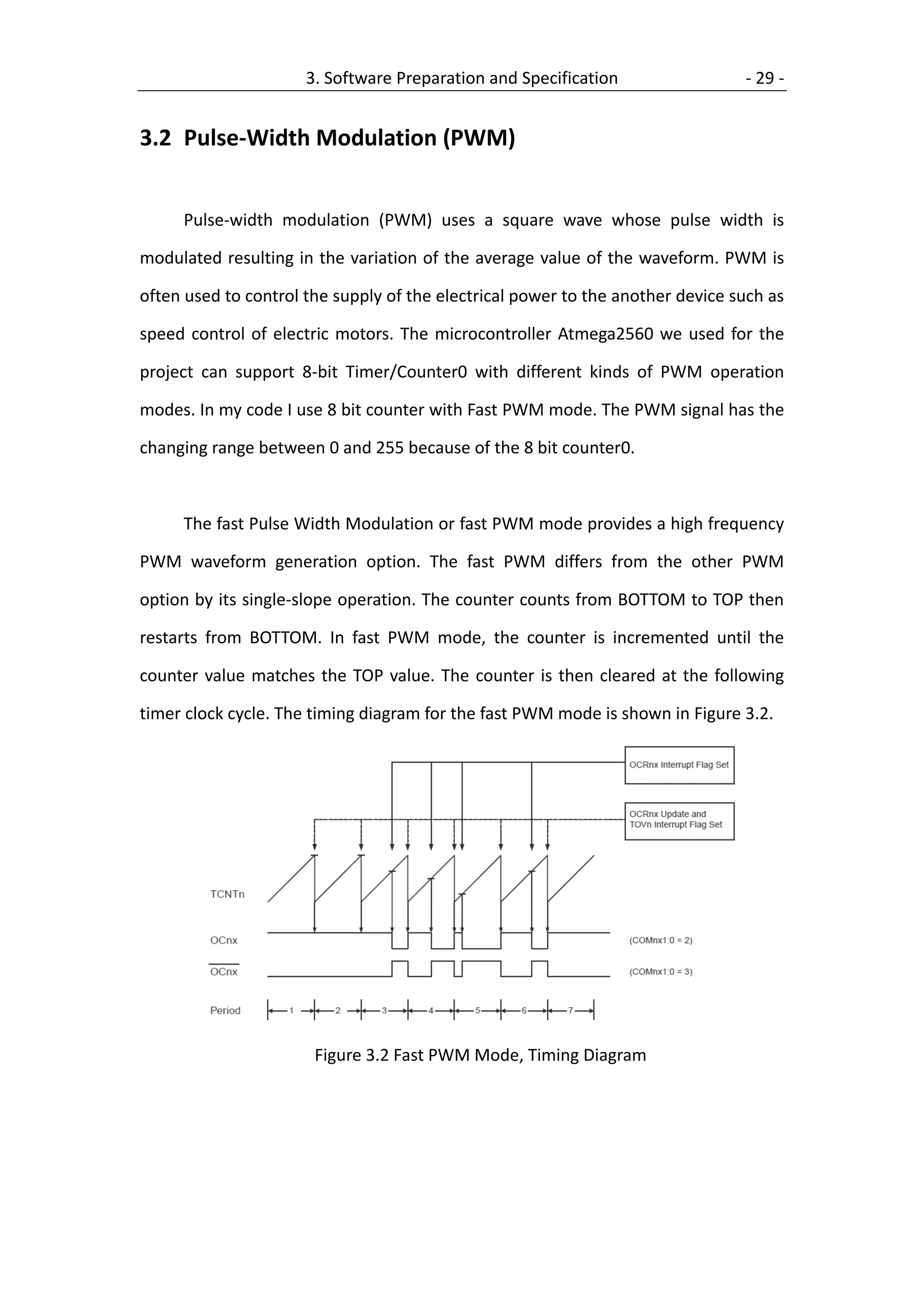
![- 30 - 3. Software Preparation and Specification
The PWM frequency for the output can be calculated by the following equation:
_/
= (3.2)
∙ (1 + 255)
_/ represents clock frequency and the variable represents the prescale
factor (1, 8, 32, 64,128, 256, or 1024). Our microcontroller equipped with a 16 MHz
crystal so _/ = 16,000,000 and the sampling frequency of IMU sensor is
100 Hz (Table 3.2), so the frequency of the control loop is also 100 Hz, then the PWM
frequency should be higher than 100 Hz so that each pulse can be fully
send inside one control loop. To fulfill this requirement the value of prescale has
been chosen equal to 256. Now the PWM frequency is calculated using (3.2) :
16,000,000
= = 244 (3.3)
256 ∙ (1 + 255)
The period of PWM signal is:
1
= = 4.096 (3.4)
→Please refer to the ATmega2560 datasheet[6] for more information on this topic.
The code can be found in “motor_init()” and “run_motor(motor,speed)”.
The function “run_motor(char motor,char speed)” send the PWM signals speed from
0 to 255 to the corresponding motor, the numbers of motor are: 1 to front rotor, 2 to
back rotor, 3 to left rotor and 4 to back rotor; speed=0 means motor stops and
speed=255 means the maximal rotational speed.
For example:
runmotor(1,255); //the front rotor rotates at maximal speed](https://image.slidesharecdn.com/2009developmentandimplementationofacontrolsystemforaquadrotoruav-111213204238-phpapp02/75/2009-development-and-implementation-of-a-control-system-for-a-quadrotor-uav-40-2048.jpg)
![3. Software Preparation and Specification - 31 -
3.3 USART Interrupt Routine
The Universal Synchronous and Asynchronous serial Receiver and Transmitter
(USART) is a highly flexible serial communication device. The ATmega2560 has four
USART’s, USART0, USART1, USART2, USART3. On the controller board RN-MEGA 2560
Model V1.0 (see www.robotikhardware.de) the USART3 is changed into the normal
[14]
USB interface to the PC . By using this interface we can send the data from
microcontroller to the software “terminal” installed on the PC and capture the data
into TXT file, and then these data can be plot by Matlab in order to compare the
experiment results with the simulation results.
The USART Transmitter has two flags that indicate its state: USART Data Register
Empty (UDREn) and Transmit Complete (TXCn). Both flags can be used for generating
interrupts. Here the UDRE3 is used for generating the data transmit flag. The UDRE3
Flag indicates whether the transmit buffer is ready to receive new data. When the
transmit buffer is full, the UDR3 interrupt is enabled and start to transmit the data,
after all the data in transmit buffer are sent, the transmit buffer is empty and the
UDR3 interrupt is disabled.
The advantage of using the interrupt routine is that the main program and the
data transmitting through serial are running in parallel, the data transmitting will not
stop the main program. Otherwise, without interrupt routine, while the transmitting
of the data, the main program will wait there until all the data has been transmitted,
which will slow down the whole program.](https://image.slidesharecdn.com/2009developmentandimplementationofacontrolsystemforaquadrotoruav-111213204238-phpapp02/75/2009-development-and-implementation-of-a-control-system-for-a-quadrotor-uav-41-2048.jpg)
![- 32 - 3. Software Preparation and Specification
According to the Table 3.4, double the USART Transmission Speed disabled
(U2X=0), the baud rate of 76800 has been chosen which has small error value
between an actual baud rate and target baud rate. With higher error the Receiver
will have less noise resistance, especially for large serial frames.
Table 3.4 Examples of UBRRn Settings for Commonly Used Oscillator
Frequencies
→Please refer to the ATmega2560 datasheet[6] for more information on this topic.
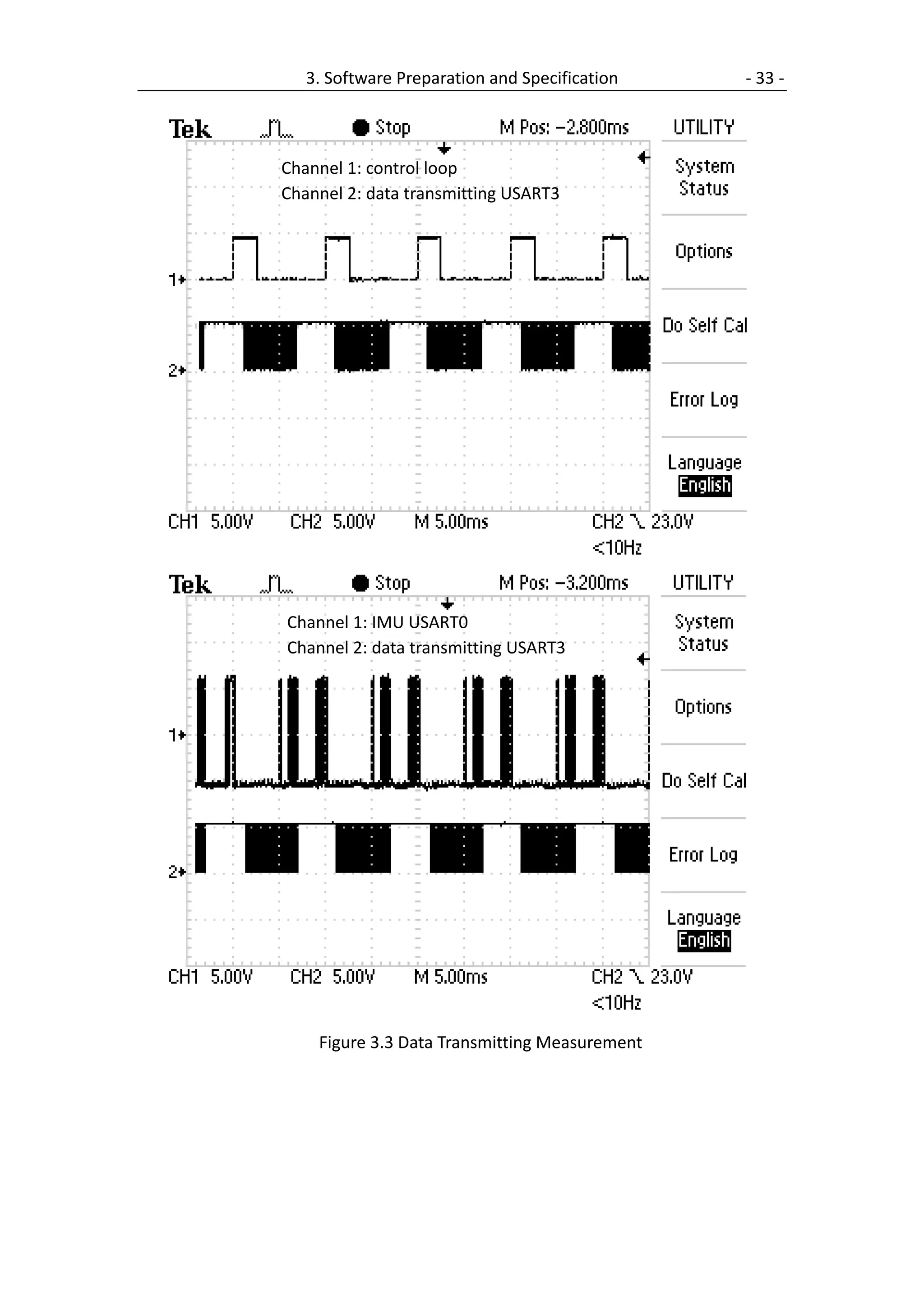
The Figure 3.3 show the data transmitting time measured by oscilloscope. From
the figures we can see the sampling time of the IMU sensor and the control loop
time are 10 ms. The data transmitting time is about 6 ms, that means every IMU data
packet is possible to be sent to PC. The code can be found in “usart3.c”.](https://image.slidesharecdn.com/2009developmentandimplementationofacontrolsystemforaquadrotoruav-111213204238-phpapp02/75/2009-development-and-implementation-of-a-control-system-for-a-quadrotor-uav-42-2048.jpg)

![Chapter 4
Quadrotor Kinematics and Dynamics
There are lots of studies and papers have described how to model the
quadrotor and since the modeling of the quadrotor is emphasis of this paper, so this
chapter will give only give the overall model of the quadrotor dynamics used for
simulation in [1]. More detailed information about modeling can be found in
[5],[11],[15],[16].
4.1 Quadrotor Kinematics
Generally, the quadrotor can be modeled with a four rotors in cross
configuration. The whole model can be considered as a rigid body. Figure 4.1
illustrates the basic motion control of the quadrotor.
Front Right
Left
Back
Figure 4.1 Quadrotor control mechanism [17]](https://image.slidesharecdn.com/2009developmentandimplementationofacontrolsystemforaquadrotoruav-111213204238-phpapp02/75/2009-development-and-implementation-of-a-control-system-for-a-quadrotor-uav-45-2048.jpg)
![- 36 - 4. Quadrotor Kinematics and Dynamics
Throttle (1 [])
The throttle movement is provided by increasing (or decreasing) all the
rotor speeds by the same amount. It leads a vertical force 1 [] with
respect to body-fixed frame which raises or lowers the quadrotor.
Roll (2 [ ∙ ])
The roll movement is provided by increasing (or decreasing) the left rotors’
speed and at the same time decreasing (or increasing) the right rotors’
speed. It leads to a torque with respect to the green axis showed in Figure
4.1 which makes the quadrotor roll. The overall vertical thrust is the same
as in hovering.
Pitch (3 [ ∙ ])
The pitch movement is provided by increasing (or decreasing) the front
rotors’ speed and at the same time decreasing (or increasing) the back
rotors’ speed. It leads to a torque with respect to the yellow axis showed in
Figure 4.1 which makes the quadrotor go forward or backward. The overall
vertical thrust is the same as in hovering.
Yaw (3 [ ∙ ])
The yaw movement is provided by increasing (or decreasing) the front-rear
rotors’ speed and at the same time decreasing (or increasing) the left-right
couple. It leads to a torque with respect to the red axis showed in Figure 4.1
which makes the quadrotor turn in horizon level. The overall vertical thrust
is the same as in hovering.](https://image.slidesharecdn.com/2009developmentandimplementationofacontrolsystemforaquadrotoruav-111213204238-phpapp02/75/2009-development-and-implementation-of-a-control-system-for-a-quadrotor-uav-46-2048.jpg)
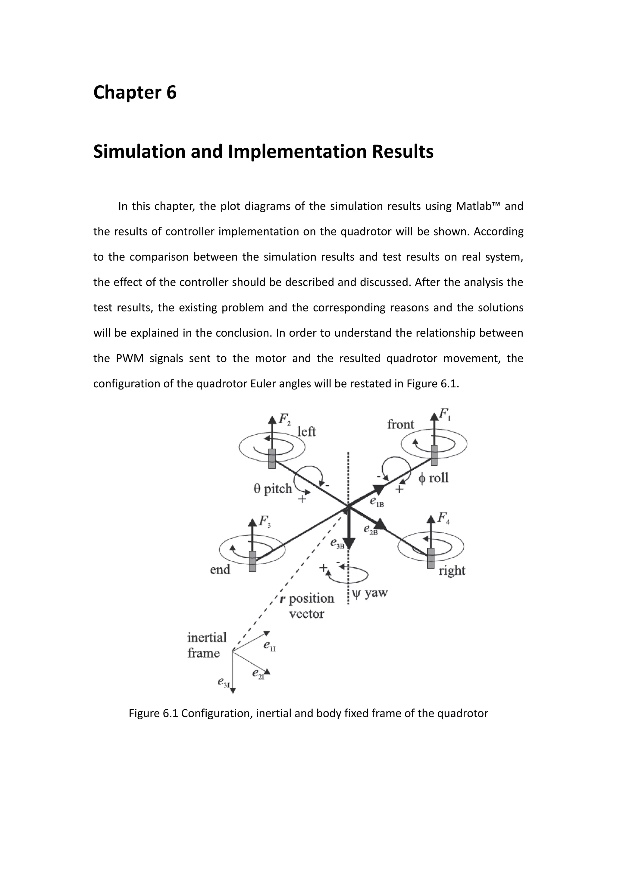
![4. Quadrotor Kinematics and Dynamics - 37 -
4.2 Quadrotor Dynamics
In order to model the quadrotor dynamics, two frames have to be defined, as
showed in Figure 4.2:
The earth inertial frame ( frame)
The body-fixed frame ( frame)
F3 F1
F2 F4
Figure 4.2 Configuration, inertial and body fixed frame of the quadrotor[1]](https://image.slidesharecdn.com/2009developmentandimplementationofacontrolsystemforaquadrotoruav-111213204238-phpapp02/75/2009-development-and-implementation-of-a-control-system-for-a-quadrotor-uav-47-2048.jpg)
![- 38 - 4. Quadrotor Kinematics and Dynamics
There are different ways to describe the dynamics of the quadrotor, such as
Euler angle, quaternion and rotational matrix. In this work the orientation of the
quadrotor is given by the three Euler angles, as mentioned in 14.1 Quadrotor
kinematics, who are roll angle , pitch angle and yaw angle , the units are
[]. These three Euler angles form the vector = (, , ). The position of the
vehicle in the inertial frame is given by the vector = , , . The transformation
of vectors from the body fixed frame to the inertial frame is given by the rotation
matrix where for example denotes cos and denotes sin :
− +
= + − (4.1)
−
The thrust force generated by rotor , =1, 2, 3, 4 is:
2
= ∙ (4.2)
where b is the thrust factor and [/] is the rotational speed of rotor . Then
the thrust force applied to the airframe from the four rotors is given by
4 4
2
= = (4.3)
=1 =1
Now the first set of differential equation that describes the acceleration of the
quadrotor can be written as:
0 0
= = ∙ 0 − ∙ ∙ 0 (4.4)
1 1
With the inertia matrix (which is a diagonal matrix with the inertias , and
on the main diagonal), the rotor inertia , the vector that describes the torque
applied to the vehicle’s body and the vector of the gyroscopic torques we
obtain a second set of differential equations:
∙ = − × ∙ − + (4.5)](https://image.slidesharecdn.com/2009developmentandimplementationofacontrolsystemforaquadrotoruav-111213204238-phpapp02/75/2009-development-and-implementation-of-a-control-system-for-a-quadrotor-uav-48-2048.jpg)
![Chapter 5
Attitude Control Algorithm Design
The attitude control loop is responsible for the generation and stabilization of a
currently required movement of the quadrotor, so that the quadrotor can also hover
in the air. Later on, other control task might be developed for the quadrotor, such as
altitude control, velocity of the quadrotor control, or the target tracking control and
landing. All those control tasks are based on the attitude stabilization of the
quadrotor. So we can consider the attitude control loop as a inner control loop which
is more faster than the others. From a control engineering point of view, this means,
the controller used for attitude control should be very fast to achieve the steady
state and also has the ability to compensate against any disturbances.
With regard to control engineering, there are many different control concepts
has been developed and studied for autonomous control of a quadrotor UAV, such
as:
Nonlinear control using feedback-linearization[1]
Nonlinear State-Dependent Riccati Equation Control[18]
Nonlinear and Neural Network-based Control[19]
PD/PD2 Controller Design[11]
Enhanced PID Controller Design[15]
and so on. In this chapter, the “Nonlinear control using feedback-linearization”
control theory has been chosen and implemented on the quadrotor to test the
results. Furthermore, the new controllers have been designed using PID control.](https://image.slidesharecdn.com/2009developmentandimplementationofacontrolsystemforaquadrotoruav-111213204238-phpapp02/75/2009-development-and-implementation-of-a-control-system-for-a-quadrotor-uav-51-2048.jpg)
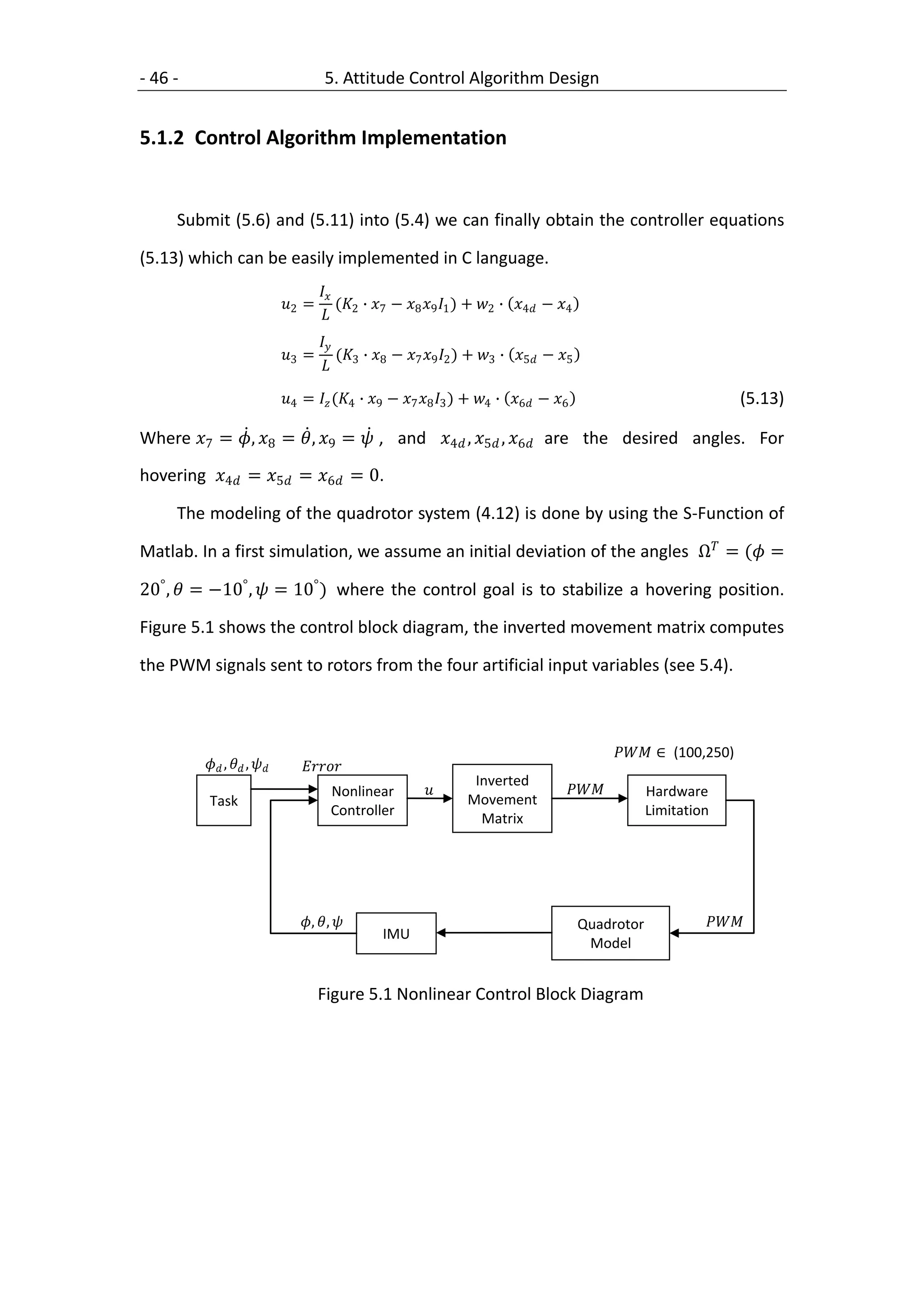
![- 42 - 5. Attitude Control Algorithm Design
The kinematics and dynamics of the quadrotor are well described in the
previous chapter. However the most important concepts can be summarized in the
set of equations (4.8) and (4.12). The state space model of the quadrotor (4.12) can
be decomposed into one subset of differential equations that describes the dynamics
of the attitude (i.e. the angles), which will be used later in this chapter for attitude
control design, and one subset that describes the translation of the UAV[1]. From
(4.12) we obtain the one subset of differential equations that describes the
quadrotor’s angular rate as:
8 9 1 − + 2
8
7
8 = 7 9 2 + 7 + 3 (5.1)
9
1
7 8 3 + 4
where we have the state variables = (, , , , , , , , ).
The artificial input variables which related the basic movement to the propellers’
squared speed are:
2 2 2 2
1 = (1 + 2 + 3 + 4 )
2 2
2 = (3 − 4 )
2 2
3 = (1 − 2 )
2 2 2 2
4 = (1 + 2 − 3 − 4 ) (5.2)
With the help of (5.1) and (5.2), we are able to design the attitude control for
the quadrotor. In the following section, different approaches of the quadrotor
attitude control design are explained and the corresponding controllers are
translated from the form in simulation software Matlab™ into implementation form
in C language. All control effect results of different controllers will be discussed in
Chapter 6.](https://image.slidesharecdn.com/2009developmentandimplementationofacontrolsystemforaquadrotoruav-111213204238-phpapp02/75/2009-development-and-implementation-of-a-control-system-for-a-quadrotor-uav-52-2048.jpg)
![5. Attitude Control Algorithm Design - 43 -
5.1 Nonlinear Control using Feedback-Linearization[1]
5.1.1 Control Algorithm Design
For design the attitude controller the influence of the gyroscopic terms is
neglected, which are comparatively small because of the small rotor inertias of the
quadrotor. Then the simplified sub model can be obtained as:
8 9 1 +
2
7
8 = 7 9 2 + 3 (5.3)
9
1
7 8 3 + 4
Now we apply a feedback linearization in order to obtain a linear system:
∗
2 = 2 7 , 8 , 9 + 2
∗
3 = 3 7 , 8 , 9 + 3
∗
4 = 4 7 , 8 , 9 + 4 (5.4)
∗ ∗ ∗
with the new input variables 2 , 3 , 4 . In order to obtain a linear system, the
following conditions must be fulfilled:
8 9 1 + , , = 2 ∙ 7
2 7 8 9
7 9 2 + , , = 3 ∙ 8
3 7 8 9
1
7 8 3 + , , = 4 ∙ 9 (5.5)
4 7 8 9
with the so far undetermined constant parameters 2 , 3 , 4 . Evaluation of (5.5)
yields the nonlinear feedback for linearization:](https://image.slidesharecdn.com/2009developmentandimplementationofacontrolsystemforaquadrotoruav-111213204238-phpapp02/75/2009-development-and-implementation-of-a-control-system-for-a-quadrotor-uav-53-2048.jpg)
![- 48 - 5. Attitude Control Algorithm Design
It is obvious that each transfer function in (5.15) has two poles at the origin.
Using the Root Locus Method to design the controller, we can place a zero using a
PD-controller to improve the dynamic behaviour of the closed loop. The is used to
obtain vertical lines as asymptotes for that branches of the root locus that converge
to infinity and to obtain two dominate stable poles. With at least one pole in the
origin the closed control loop of the system has no steady-state error. [20] The root
locus graph is shown in following figure.
Figure 5.2 Root Locus using simple PD Controller
Now we have the simple PD controller for roll, pitch and yaw control with the form:
= + ∙ () (5.16)
with is the parameter of the proportional part and is the parameter of the
differential part. Since the real control loop is not a time continuous system but with
the sampling time of 0.01 . Thus in Matlab simulation we use discrete PID
control for continuous plant [21].](https://image.slidesharecdn.com/2009developmentandimplementationofacontrolsystemforaquadrotoruav-111213204238-phpapp02/75/2009-development-and-implementation-of-a-control-system-for-a-quadrotor-uav-58-2048.jpg)
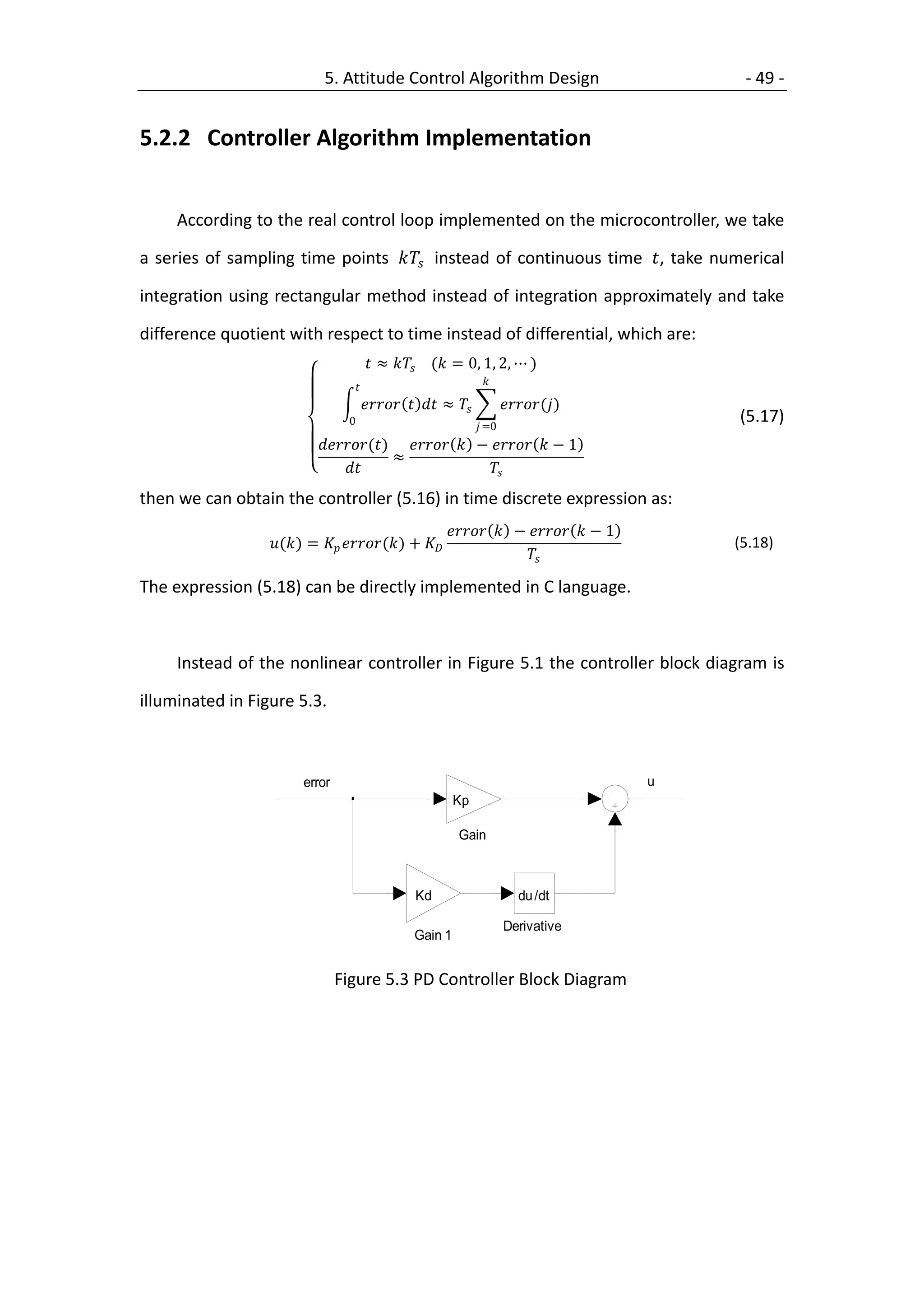
![- 50 - 5. Attitude Control Algorithm Design
5.3 PD controller Design with Partial Differential
Instead of the simple PD controller, the PD controller with Partial differential is
more widely used in industry area because of its better performance. Hence here we
also design a new PD controller with partial differential based on the simplified
system (5.15).
5.3.1 Controller Algorithm Design
In PID control theory, the introduce of the differential part can improve the
dynamic characteristic of the system, but also make the system easily be disturbed by
the high frequency signal, the drawback of the differential part is especially obvious
when the error signal has a big disturbance. However, the system performance can
be improved by adding a low pass filter to the control algorithm.
To overcome the drawback described above, one way is that adding a first order
inertial element (low pass filter) = 1 (1 + ) , which can improve the
system performance. The structure of the PD controller with partial differential is
shown in Figure 5.4, the low pass filter is added after the PD controller.[21]
() 1 ()
+
+ 1 + ∙
∙
Figure 5.4 Block Diagram of PD Controller with Partial Differential](https://image.slidesharecdn.com/2009developmentandimplementationofacontrolsystemforaquadrotoruav-111213204238-phpapp02/75/2009-development-and-implementation-of-a-control-system-for-a-quadrotor-uav-60-2048.jpg)
![5. Attitude Control Algorithm Design - 51 -
If we rearrange the PD controller shown in Figure 5.4 we can obtain the PD
controller in the form:
() 1 +
= = (5.19)
() 1 +
with = and ≪ . The controller (5.19) is so called real
PD-controller[20] and using the Root Locus method this controller is simply placing
one real zero near to the origin as a dominate pole and placing one real pole far away
from the added zero on the negative real axis of the Root Locus graph. Now we
obtain the Root Locus diagram as shown in Figure 5.5.
−
−
Figure 5.5 Root Locus using PD Controller with Partial Differential](https://image.slidesharecdn.com/2009developmentandimplementationofacontrolsystemforaquadrotoruav-111213204238-phpapp02/75/2009-development-and-implementation-of-a-control-system-for-a-quadrotor-uav-61-2048.jpg)
![- 54 - 5. Attitude Control Algorithm Design
1 1 0 0 0
2 0 2 0 0
= =
3 0 0 3 0
4 0 0 0 4
From (5.25) and (5.26) we can get
= −1 ∙ −1 ∙ − (5.27)
The (5.27) can be rewritten as:
1 1 1
1 = 1 + 3 + − 1
1 4 2 4 4
1 1 1
2 = 1 − 3 + − 2
2 4 2 4 4
1 1 1
3 = 1 + 2 − − 3
3 4 2 4 4
1 1 1 (5.28)
4 = − − − 4
4 4 1 2 2 4 4
The set of equations (5.28) can be easily implemented in C language to calculate
the desired PWM signals. Take into account that the operating range of the motor
speed ∈ (100, 250) for attitude control, it’s necessary to limit the value of
controller output variable with 2 ∈ −0.8, 0.8 , 3 ∈ −0.8, 0.8 [] and
4 ∈ −0.3, 0.3 []. This hardware limitation is always added to the controller in the
implementation test. The operating range of PWM signals for each are not the same
because there are big difference between the performances of the motors, see Table
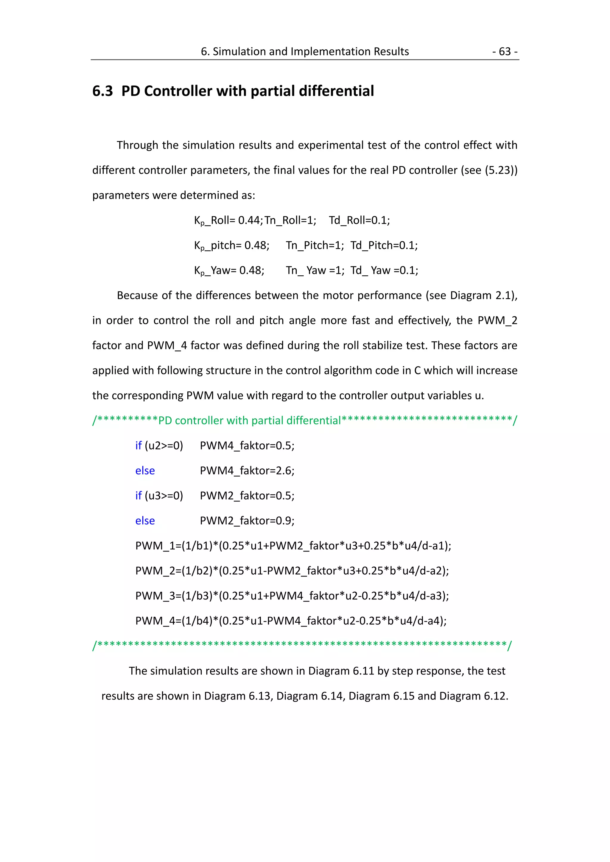
2.1 Motor Lift Force Measurement.](https://image.slidesharecdn.com/2009developmentandimplementationofacontrolsystemforaquadrotoruav-111213204238-phpapp02/75/2009-development-and-implementation-of-a-control-system-for-a-quadrotor-uav-64-2048.jpg)
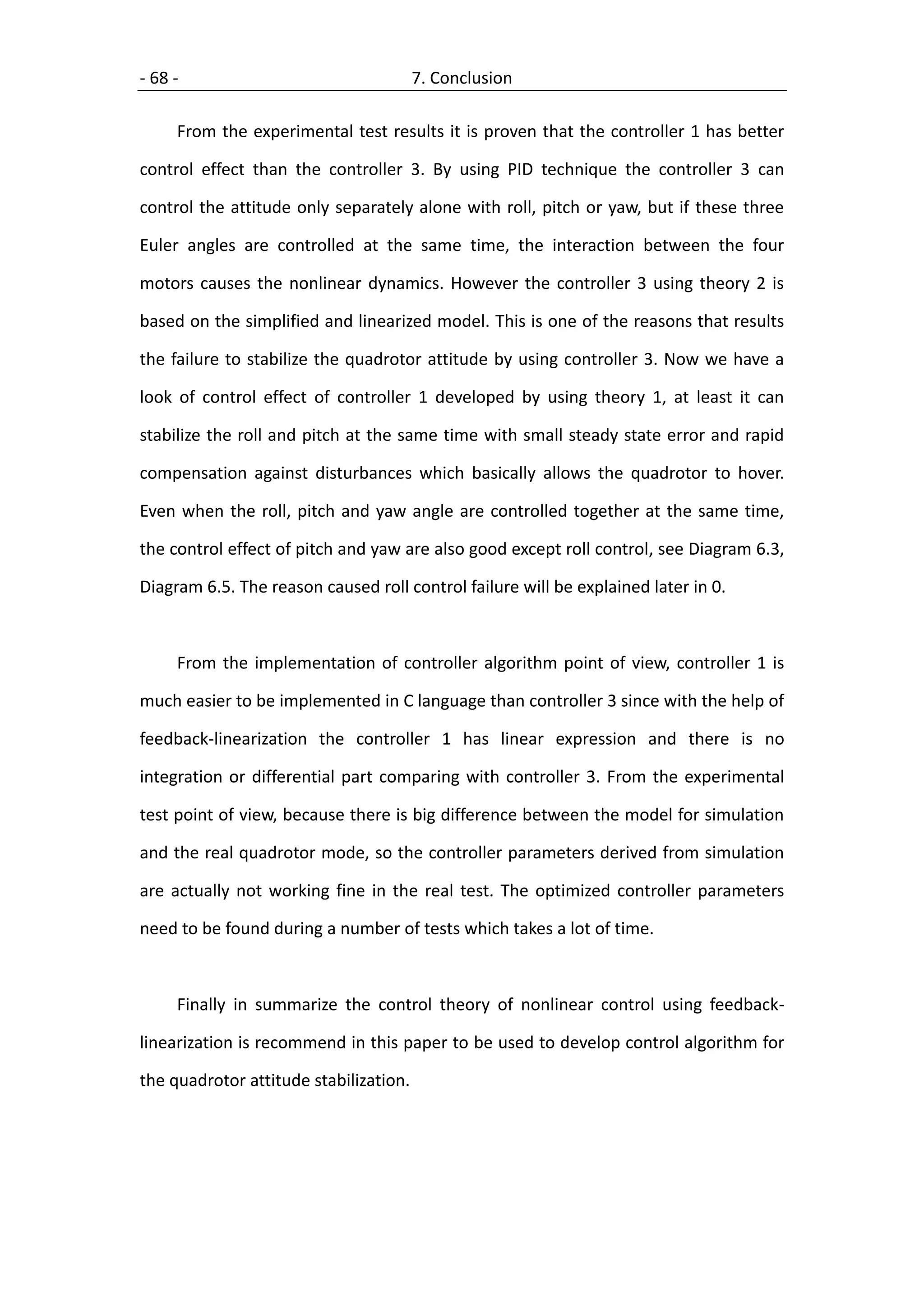
![7. Conclusion - 71 -
Redesign the mechanical structure of the quadrotor
The mechanical structure I designed in this project is only for the first step
test, it's a little heavy and the connection between the test platform and
the quadrotor is not with same length in X and Y direction which actually
results the inertia value of ≠ . This also leads to the different control
effects which are unexpected for roll and pitch control.
Identify the quadrotor constants by experiments
The nonlinear controller depends a lot on the accuracy of the quadrotor
constants. If the quadrotor constants are more accurate and close to the
real model, it will help the quadrotor to have better attitude control
performance by using nonlinear controller. The experiments to determine
the quadrotor constants are described in paper [11].
Besides above mentioned works related to improvement of attitude control, the
quadrotor provide interesting control challenges and impressive application
possibilities. Based on this attitude control, the other more advanced control task
can be implemented such as velocity control by using Inertial Navigation System
(INS)[1] , height sensor to control the altitude, GPS sensor to control the position,
wireless video sensor used for target tracking and so on. Although there has not
been any fully autonomous quadrotor flight possible to date, there are still other
groups who will continue to work on the quadrotor project to finally realize the
autonomous flight.](https://image.slidesharecdn.com/2009developmentandimplementationofacontrolsystemforaquadrotoruav-111213204238-phpapp02/75/2009-development-and-implementation-of-a-control-system-for-a-quadrotor-uav-81-2048.jpg)

![- 73 -
List of Figures
Figure 1.1 Timeline illustrating Course of Events .............................................. - 4 -
Figure 2.1 Hardware Architecture for real-time application [5] ………..............- 9 -
Figure 2.2 Robostix Board ................................................................................. - 9 -
Figure 2.3 Gumstix ............................................................................................ - 9 -
Figure 2.4 Wifistix ............................................................................................. - 9 -
Figure 2.5 The main process interacting with peripheral components [5] ...... - 10 -
Figure 2.6 DraganFlyer .................................................................................... - 11 -
Figure 2.7 Hardware Architecture MicrocontrollerOnBoard Implementation - 13 -
Figure 2.8 Mechanical Structure of Quadrotor ............................................... - 14 -
Figure 2.9 Test Platform .................................................................................. - 15 -
Figure 2.10 MTi Overview ............................................................................... - 16 -
Figure 2.11 MTi with sensor-fixed co-ordinate system overlaid..................... - 17 -
Figure 2.12 Electronic circuit board ................................................................ - 19 -
Figure 2.13 Motor controller Board ................................................................ - 20 -
Figure 2.14 Motor Force Experiment .............................................................. - 21 -
Figure 3.1 IMU Message Structure ………………………………………………………..- 25 -
Figure 3.2 Fast PWM Mode, Timing Diagram ................................................. - 29 -
Figure 3.3 Data Transmitting Measurement ................................................... - 33 -
Figure 4.1 Quadrotor control mechanism [17]……………………….……………………..- 35 -
Figure 4.2 Configuration, inertial and body fixed frame of the quadrotor[1] .. - 37 -
Figure 5.1 Nonlinear Control Block Diagram…………………………………..……………- 46 -
Figure 5.2 Root Locus using simple PD Controller .......................................... - 48 -
Figure 5.3 PD Controller Block Diagram .......................................................... - 49 -
Figure 5.4 Block Diagram of PD Controller with Partial Differential ............... - 50 -](https://image.slidesharecdn.com/2009developmentandimplementationofacontrolsystemforaquadrotoruav-111213204238-phpapp02/75/2009-development-and-implementation-of-a-control-system-for-a-quadrotor-uav-83-2048.jpg)
![- 77 -
Bibliography
[1]. H. Voos, “nonlinear Control of a Quadrotor Micro-UAV using
Feedback-Linearization”, University of Applied Science Ravensburg-
Weingarten, Germany
[2]. Katsuhiko Ogata, Modern control engineering, 4. edition, IBSN
0-13-043245-8, 2002
[3]. Schmitt Günter, Mikroconputertechnik mit Controllern der Atmel
AVR-RISC-Familie, ISBN 978-3-486-58400-4, 2007
[4]. T. Goclel, R. Dillmann, Embedded Robotics, ISBN 3-89576-155-9, 2005
[5]. J. Bjø M. Kjærgaard, M. Sø
rn, rensen, “Autonomous Hover Flight for a Quad Rotor
Helicopter”, Automation and Control Department of electronic systems,
AALBORG University, Denmark, 2007
[6]. MT Software Development Kit Documentation, Xsens Technologies B.V. ,
Revision F, Feb. 21, 2007, www.xsens.com
[7]. MTi and MTx Low-level communication Documentation, Xsens Technologies
B.V., Revision F, Sep. 20, 2007, www.xsens.com](https://image.slidesharecdn.com/2009developmentandimplementationofacontrolsystemforaquadrotoruav-111213204238-phpapp02/75/2009-development-and-implementation-of-a-control-system-for-a-quadrotor-uav-87-2048.jpg)
![- 78 -
[8]. Mti and MTx User Manual, Xsens Technologies B.V., Revision I, Jan. 30, 2007,
www.xsens.com
[9]. Df5ti-manual, draganFly Innovations Inc, www.rctoys.com
[10]. „BTS 621 L1“ motor controller datasheet, SIEMENS Semiconductor Group
[11]. A. Tayebi, S. McGilvray, Attitude stabilization of a four-rotor aerial robot, in
Proc. of 43rd IEEE Conf. on Decision and Control, Atlantis, Paradise Island,
Bahamas, 2004
[12]. M. Binswanger, Autonomous Airship, Development of a Navigation- and
Control-unit for a Airship Model, University of Applied Science Ravensburg-
Weingarten, March 2008
[13]. ATmega2560 datasheet, ATMEL, 2549l-AVR, July 2006, www.atmel.com
[14]. RN-MEGA 2560 Modul V1.0 datasheet, robotikhardware.de, Feb. 05, 2007
[15]. T. Bresciani, “Modeling, Identification and Control of a Quadrotor
Helicopter”, Department of Automatic Control, Lund University, October
2008
[16]. S. Bouabdallah, P.Murrieri, R. Siegwart, “Design and Control of an Indoor
Micro Quadrotor”, in Proc. Of the Int. Conf. on Robotics and Automation
ICRA’ 2004, New Orleans, USA, 2004](https://image.slidesharecdn.com/2009developmentandimplementationofacontrolsystemforaquadrotoruav-111213204238-phpapp02/75/2009-development-and-implementation-of-a-control-system-for-a-quadrotor-uav-88-2048.jpg)
![- 79 -
[17]. Beau J. Tippetts, “Real-time implementation of vision algorithms for control,
stabilization, and target tracking, for a hovering micro-UAV”, Brigham Young
University, August 2008
[18]. H. Voos, “Nonlinear State-Dependent Riccati Equation Control of a
Quadrotor UAV”, In Proc. of the IEEE Trans. on Control Systems Technology,
VOL.12, No.4, July 2004
[19]. H. Voos, Nonlinear and Neural Network-based Control of a small Four-Rotor,
in Proc. of the IEEE/ASME Int. Conference on Advanced Intelligent
Mechatronics, Zurich, CH, 2007
[20]. H. Voos, Advanced Control, University of Applied Science
Ravensburg-Weingarten, 2008
[21]. J. Liu, Advanced PID Control Matlab Simulation (second edition), Publishing
House of Electronics Industry, Beijing, China, Mai 2007
[22]. Jie Chen, Matlab User Guide, Publishing House of Electronics Industry,
Beijing, 2008](https://image.slidesharecdn.com/2009developmentandimplementationofacontrolsystemforaquadrotoruav-111213204238-phpapp02/75/2009-development-and-implementation-of-a-control-system-for-a-quadrotor-uav-89-2048.jpg)