The document summarizes a master's thesis that analyzes and develops controllers for a quadcopter. It presents the dynamic equations of the quadcopter and linearizes them. Two backstepping controllers are developed - a simpler one that cannot absorb disturbances, and a more advanced one that can handle disturbances like changes in mass. Both controllers separate attitude from horizontal/vertical position control. The controllers are simulated and compared to evaluate their performance.
![Chapter 1
Introduction
Quadcopters and their control have being developed in the last 20 years by
many investigation groups all around the world. However, it was only when
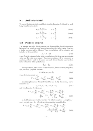
the size, consumption and weight of the computers were reduced, when these
aircraft became popular. Nowadays, their use is being regularized gradually in
many countries and it is expected that they will be used in several civil uses in
a near future.
There are presently a wide variety of techniques that may be used to control
them. In [24] a review of a wide set of different controllers, with their advantages
and their drawbacks, is presented. Normally, the quadcopter’s control is divided
in two different levels; one low level controller, in charge of stabilizing the atti-
tude, and a high level one, in charge of controlling the horizontal position. The
vertical movement can be separately controlled.
Linear strategies, and more specifically the well-known PID controllers, may
provide acceptable results if the movement of the quadcopter is slow and close
to the equilibrium point (hovering). For instance, in [16], the attitude of the
quadcopter was stabilized using a PID controller, whereas in [17] the attitude
and the position were controlled by this type of controller. In many cases, the
parameters are tuned intuitively by just observing the system response.
PID controllers can be combined with other methods to improve their per-
formance. In [22] for example, an helicopter was controlled with a PID, which
is switched to different configurations depending on the aircraft’s state. This is
actually an adaptive method, since its configuration changes depending on the
environment and/or the aircraft state. In that case, an adaptive method was
use to improve the robustness of the controller, but also if the system presents
not-well-known characteristics, they might be useful. In [7] for instance, the sys-
tem was supposed to have uncertain mass, inertia and aerodynamic damping
coefficients and the controller was able to deal with these uncertainties.
Another widely used and well-known technique is the backstepping. It con-
sists of dividing the system in different levels and stabilizing them one by one
progressively. In [15], using a quatiernion formulation, a backstepping method
was implemented to stabilize the attitude of the quadcopter, and Lyapunov
functions to prove the stability of the system. To improve the robustness of a
backstepping controller, in [9] an integrator term was added, eliminating steady-
state errors and reducing the response time.
Linear-Quadratic Regulators (LQR) have been also studied. In [2], a PID
1](https://image.slidesharecdn.com/520123f2-eb82-4c72-acd5-0cf972ce5fd0-150625092845-lva1-app6892/85/Control-of-a-Quadcopter-3-320.jpg)
![and a LQR controller are compared. The LQR one, which was based on a more
complex model, presents better results. Also feedback linearization [19], robust
control [3] and intelligent techniques [20][8] are used. Even really demanding
controllers in terms of computation cost can now be implemented due to the
improve in the micro-computers in the last years, like predictive control tech-
niques [5]. Despite here only a couple of techniques have been named, one can
get a picture of the diversity of solutions available to control these systems.
In this work, two different backstepping methods are presented and com-
pared. These methods converge fast and need less computational efforts, but
normally their robustness is not specially good. Both controllers separate the
attitude control from the horizontal and vertical position control. In first place,
the attitude is stabilized to lead the quadcopter to the required angles, by
controlling the traction of the propellers. The horizontal position control is sta-
bilized in second place, by assuming that the attitude angles are the variables
that can be controlled. The first and more simple controller is not able to ab-
sorb disturbances, such as horizontal forces or changes in the mass; the second
and more advance one, is capable of handle them. A final comparison will show
these differences.
2](https://image.slidesharecdn.com/520123f2-eb82-4c72-acd5-0cf972ce5fd0-150625092845-lva1-app6892/85/Control-of-a-Quadcopter-4-320.jpg)
![Faero, Maero aerodynamic forces and moments
Fprop, Mprop the propulsive forces and moments (propellers’ traction)
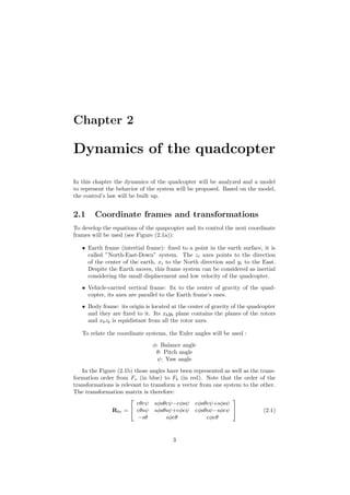
Every term will be determined in the following subsections.
2.2.1 Aerodynamic forces and moments
In a first approximation, they will be considered as negligible, i.e. Faero ≈
Maero ≈ 0. As the quadcopter moves faster, the aerodynamic forces become
higher and make it to move slower. If fact, if we simulated the movement of
the quadcopter without having these forces into account, it would accelerate
indefinitely, which is clearly unrealistic. Anyway, in this work only slow a dis-
placements will be considered and therefore this approximation can be assumed.
2.2.2 Propulsive forces
They are generated by the traction of the 4 propellers installed in the quad-
copter. The forces’ direction is always −zb, are always positive and it will be
assumed that they do not depend on the relative velocity of the air respect each
propeller1
. Therefore, the transfer function of the traction of each propeller, ui,
will be assumed to be:
ui = µ
ωm
s + ωm
vmi
(2.5)
where µ is a constant given, ωm is a bandwidth and vmi
is the voltage
delivered to the engines. In the Figure (2.2) the traction of each propeller and
the direction of rotation have been represented. The total force, resulting from
adding the traction of each propeller, is then T = u1 + u2 + u3 + u4. Normally
a change of variable is used so that the problem is simplified:
u1 + u2 + u3 + u4 = uz (2.6)
2.2.3 Propulsive moments
The moments caused by the traction of the propellers are:
Mx = L = d(u4 − u2) (2.7a)
My = M = d(u1 − u3) (2.7b)
Nz = N = dN (u1 + u3 − u2 − u4) (2.7c)
where d is the distance from the center of the propeller to the CoG in the xbyb
plane and dN is a fictitious distance which represents the aerodynamic reaction
of the propellers due to the draft of the blades. Note that the rotation inertia
of the blades and the motors have been neglected, which will cause moments
1The behavior of the propeller depends highly on it, see [14]. However, such a relative
velocity might be assumed to be much lower than the relative velocity of the air due to the
spin of the blades.
5](https://image.slidesharecdn.com/520123f2-eb82-4c72-acd5-0cf972ce5fd0-150625092845-lva1-app6892/85/Control-of-a-Quadcopter-7-320.jpg)
![z[m]
-1
-0.5
0
φ[°]
0
10
20
θ[°]
0
10
20
time [s]
0 5 10 15 20 25 30 35 40
ψ[°]
0
20
40
60
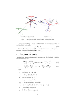
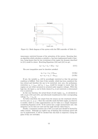
Figure 4.3: Response of the system with step reference signals.
.
21](https://image.slidesharecdn.com/520123f2-eb82-4c72-acd5-0cf972ce5fd0-150625092845-lva1-app6892/85/Control-of-a-Quadcopter-23-320.jpg)
![time [s]
0 20 40 60 80 100 120
-1
-0.5
0
0.5
1 X
Y
Z
(a) Position of the quadcopter in inertial
frame coordinates
Y [m]
1
0.5
0
10.80.6
X [m]
0.40.20-0.2
1.2
0
0.2
0.4
0.6
0.8
1
-Z[m]
(b) Trajectory of the quadcopter
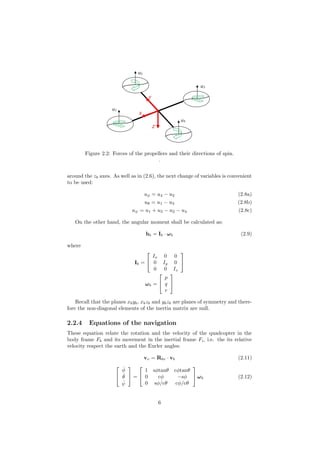
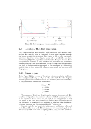
Figure 4.4: Test of the 6dof controller, following a predefined trajectory
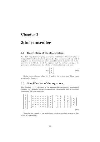
4.3 Results of the 6dof controller
In order to test that the controller works properly, the quadcopter will be com-
manded to reach some points in the space with a specific orientation. Firstly, the
quadcopter will ascend to zi = −0.5 m and then trace a 1-meter-side square in
the space with an orientation of ψd = 0. Having completed that, it will change
its orientation to ψd = π/4 and repeat the same movement in the space but
with an altitude of zi = −1. Despite the orientation changes, the quadcopter
must be capable of reaching the points anyway.
The movement of the quadcopter has been represented in Figure 4.4, follow-
ing the trajectory above described. In the Figure 4.4a the position in inertial
frame coordinates are shown; once the quadcopter reaches zi = −0.5 m, it
moves forward and then to the left, coming back to the origin. Afterwards,
it changes again its high to zi = −1 m and its orientation to ψd = π/4 and
repeats the same movement. Note that even with the change in the orientation
the quadcopter reaches the destination points successfully. In the Figure 4.4b
the 3d movement, estimated by the Observer, has been represented, indicating
the orientation with the blue arrows at some points of the trajectory.
Considering a step input of 1 m, see Figure 4.4a, the time characteristics of
the system response in the x and y direction are:
maxover = 0
td = 1.58 s
tr = 3.72 s
ts = 5.51 s
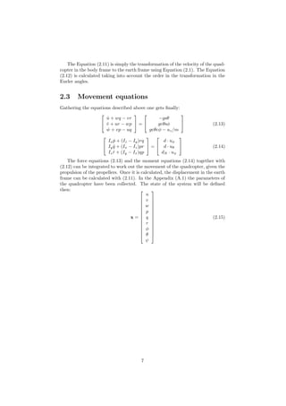
The attitude and the input of the motors haven represented in Figure 4.5a
and 4.5b respectively. The change in the pitch and roll angles needed to reach
the velocities in every direction are actually small (∼5◦
) so that the linealized
system is closed to the real one. On the other hand, once the yaw angle changes,
the distribution of pitch and roll angles change as well to achieve the attitude
to reach the destination points in the second level of the travel (in the plane
zi = −1). As it can be seen in the Figure (4.5b) the inputs remains always
23](https://image.slidesharecdn.com/520123f2-eb82-4c72-acd5-0cf972ce5fd0-150625092845-lva1-app6892/85/Control-of-a-Quadcopter-25-320.jpg)
![time [s]
0 20 40 60 80 100 120
angle[°]
-10
0
10
20
30
40
50
φ
θ
ψ
(a) Attitude (Euler angles)
time [s]
0 20 40 60 80 100 120
Vm[V]
0
2
4
6
8
10
12
14
16
18
20
Vm1
Vm2
Vm3
Vm4
(b) Inputs to the motors
Figure 4.5: Attitude and inputs during the movement represented in Figure
(4.4b)
between their limits, 0 and 20 V.
24](https://image.slidesharecdn.com/520123f2-eb82-4c72-acd5-0cf972ce5fd0-150625092845-lva1-app6892/85/Control-of-a-Quadcopter-26-320.jpg)
![Chapter 5
Advanced backstepping
controller
A new a more advanced controller will be presented, which is based on the
backstepping technique, but is build up with more complex laws, capable of
absorbing external forces and changes in the mass. This controller is presented
in [9] and the main contribution of this work is how the parameters have been
selected by using a genetic algorithm.
First, we define a new frame coordinate system k, whose center is the center
of gravity of the quadcopter, its x axes correspond to the k2 axes (see Figure
2.1b), y axes is k1 and z is zv. The angular velocity of this new system is
the ωk = [0, 0, − ˙ψ] so that it can be neglected in Equation (2.3), since it can
be expected only low values of yaw velocities. Taking the state of the system
of Equation (2.15) represented in the frame k, the equation of the motion is
˙x = f(X, U), being
f(X, U) =
uz·Ux+Dx
m
uz·Uy+Dy
m
−uz·cos φ cos θ
m + Dz
m + g
Iy−Iz
Ix
rq + d
Ix
· uφ
Iz−Ix
Iy
pr + d
Iy
· uθ
Ix−Iy
Iz
qp + dN
Iz
· uψ
p
q
r
(5.1)
where Di are disturbances, in N, in every axes; ux and uy are the coefficients
to project the traction in both axes:
−ux = cos φ sin θ cos ψ + sin φ sin ψ (5.2a)
−uy = cos φ sin θ sin ψ − sin φ cos ψ (5.2b)
25](https://image.slidesharecdn.com/520123f2-eb82-4c72-acd5-0cf972ce5fd0-150625092845-lva1-app6892/85/Control-of-a-Quadcopter-27-320.jpg)
![Now, lets divide again the term ux2 into two, ux2 = ux3 + ux4, and taking
ux3 = ˙pxλx + ˙e1xc1x, we get:
˙V = ˙px
∂V
∂px
+ ˙e1x
∂V
∂e1x
− ux4
∂V
∂e2x
−
˜Dx
m
∂V
∂e2x
−
˙ˆDx
∂V
∂ ˜Dx
(5.20)
The last term can be chosen as:
ux4 =
˙px
∂V
∂px
+ ˙e1x
∂V
∂e1x
∂V
∂e2x
+ kx
∂V
∂e2x
and as result, the derivative is:
˙V = −kx
∂V
∂ex2
2
−
˜Dx
m
∂V
∂ex2
−
˙ˆDx
∂V
∂ ˜Dx
(5.21)
We still have to choose the law of the estimated perturbation and the depen-
dency of the function V on ˜D. If we take:
˙ˆDx = −γx
∂V
∂ex2
(5.22)
∂V
∂ ˜Dx
=
˜Dx
mγx
(5.23)
both terms cancel each other, having finally:
˙V = −kx
∂V
∂ex2
2
(5.24)
which is definite-negative, being the convergence ensured. To define the control
terms u1 and u4 and the perturbation law ˆD, the partial derivative ∂V
∂ex2
must
be chosen:
∂V
∂ex2
= βx1px + βx2ex1 + βx3ex2 (5.25)
The Lyapunov function is then, considering also Equation (5.23)
V = β1xpxe2x + β2xe1xe2x + β3xe2
2x +
˜D2
x
2mγx
+ (·) (5.26)
Note that the last term of the function has not been specified, since it is
not needed to determine the control and the perturbation law. However, to
ensure the convergence of the system, with the explicit construction of the Lya-
punov functions, it must be shown that V is definite-positive. Here, a Implicit
Lyapunov Function (ILF, see [1]) has been used so that it is not necessary to
explicitly specified it1
. The control law is then:
ux =
m
u1
¨xd − ˆDx + ˙pxλx + ˙e1xc1x +
β1x ˙px + β2x ˙e1x ˙e2x
β1xpx + β2xe1x + β3xe2x
kx(β1xpx + β2xe1x + β3xe2x) (5.27)
1In the paper where this controller is developed [9] is not explicitly proved the convergence
of the system, since a function g(V, X) must have been specified.
28](https://image.slidesharecdn.com/520123f2-eb82-4c72-acd5-0cf972ce5fd0-150625092845-lva1-app6892/85/Control-of-a-Quadcopter-30-320.jpg)
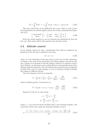
![5.4 Parameter selection
5.4.1 Use of genetic algorithms
One of the goals pursued when designing a controller is that it is easy to tune,
and one of the characteristics of the easy-to-tune controllers is normally that
they have a reduced number of parameters. Having a look on the controller just
presented, one can realized that it is not the case at all. Note that the controller
presented in Section 4 only has 6 parameters in the low level controller and 2
more for the high level one.
For the attitude control, we have a total of 3 parameters for every axes,
and 1 more if we consider the limit to start using the integral term of the con-
trol. Considering that the controller for θ and φ will have the same parameters
because of symmetry reasons, there are 8 parameters to be chosen:
c1θ,φ
c2θ,φ
λθ,φ eθ,φ
λlim
(5.42a)
c1ψ
c2ψ
λψ eψ
λlim
(5.42b)
The situation in the position controller is even worst. For the x and y
position control, we have a total number of 8 parameters, having taken into
consideration that for both axis the controller has the same configuration and
that the perturbation ˆD has its own law:
c1x,y
λx,y ex,y
λlim
kx,y γx,y β1x,y β2x,y β3x,y (5.43)
In the case of altitude control, we have 4 parameters, and 2 more for the
perturbation and the mass estimation:
λz ez
λlim
γ1z γ2z c1z c2z (5.44)
In total, the controller requires on 22 parameters to be specified. Note that
he control laws are quite complicated and it would be very tricky to analytically
draw conclusions about how the parameters influence the response of the system,
even if the model is simplified by a linearization, for example. Knowing that,
non-so-conventional approaches must be consider.
The use of intelligent system, and more particularly the evolutionary algo-
rithms (EA), have been used in the control theory in the last 30 years, see[11].
The EA enclose a set of techniques in which one can underline evolutionary pro-
gramming, evolution strategies, genetic programming and genetic algorithms.
Genetic algorithms (GA) are methods for robust search and optimization
based on natural selection principles and population genetics. Basically they
try to look for a sub-optimal solution of a problem when the number of possible
parameters or solutions make impossible scan them properly because computa-
tional costs. GA were popularized by Goldberg in 1989 and are the most used
method for control purposes, followed by genetic programming. Its two main
uses in the control theory are off-line design and the on-line optimization, being
the first one way more used since the the difficulties using the on-line design
associated with using them in real time.
In the search of a sub-optimal solution, a evaluation or fitting function must
be proposed so that the algorithm objectively verifies how good a solution is.
This function represents then the desired objectives of the solution and it might
31](https://image.slidesharecdn.com/520123f2-eb82-4c72-acd5-0cf972ce5fd0-150625092845-lva1-app6892/85/Control-of-a-Quadcopter-33-320.jpg)
![take into account penalties for not wanted behaviors. In case we have more
than one objective to be fulfilled, the problem becomes harder, since only one
scalar value is to be used to distinguish between good and bad solutions. One
can try to integrate both evaluation function into only one, taking into account
the importance of each objective by means of weights, see [12].
GA have been used to optimize the PID parameters of the controllers in
different fields from the 90s (see [21] and [23] for instance), but also in the H-
infinity and LQG control (see [6]), among others. Particularly they have been
implemented to tune the PID controller of a quadcopter in [10] and even as
a methodological method of designing UAVs in [18]. However, in the field in
which GA have been widely implemented for UAVs, is in the path planning,
optimal routing and strategical and tactical planning.
In general, we can find the following elements when using this method:
• Initial population: it is the set of solutions proposed initially. They can
be seeded on the search space randomly, uniformly spaced, heuristically,
with good solutions which are previously known or a combination of them.
Normally in a number between 20 and 100, this number is preserved along
the generations. Also the so called islands can be used, which are groups
of populations which progress in parallel and can interchanged genetic
material in punctual moments.
• Representation: we have to distinguish two different concepts or do-
mains. On one hand, we have the genotype space, which is the represen-
tation of the parameters to be optimized so that the algorithm is able
to manipulate them. In the early beginning, a binary representation was
usually implemented, but real numbers or any other data structure can be
also used. On the other hand, we have the phenotype space, which is the
real space of the parameters in the model, normally real numbers. The
transformation from the phenotype to the genotype is called encoding,
whereas the other way around is called decoding.
• Evaluation: every generation of solutions must be evaluated in order to
know how they are fulfilling an objective. A fitness value, which measures
the performance of each member is normally used and the the complete
generation can be ordered in a ranking. Note that it is necessary to finally
obtain a single scalar value, either absolute of relative to the rest of the
members of the generation.
• Selection: once the current population has been evaluated, the next step
is to select the members which are going to produced the next generation of
solution. The tournament method consist of once group of pairs have been
selected, they compete between them and the genetic material form the
winner will be then used. The roulette wheel is on the contrary a method
in which the parents are chosen randomly with a probability proportional
to the fitness value, i.e. the better the fitness value is, the higher the
probabilities of being chosen as parent is. Beside these two methods,
there exists many other, such as the stochastic universal sampling or the
truncation selection.
• Recombination: or crossover, is how the parents interchange their ge-
netic material and its a crucial feature in the GA. There are multiple ways
32](https://image.slidesharecdn.com/520123f2-eb82-4c72-acd5-0cf972ce5fd0-150625092845-lva1-app6892/85/Control-of-a-Quadcopter-34-320.jpg)
![of carrying it out; for instance, complete pieces of genes can be taken ran-
domly from one of the parents, or the complete chain of genes can be
split and interchanged between them. Often the frequency with which the
genetic material is interchanged is reduced when generations go by. The
new members are called offspring.
• Mutation: after the recombination, a mutation might be considered,
which is a random change in one of the genes. It allows to randomly
explore other search spaces, which might have been discarded, and gives a
chance to recover good genetic material. The probability of the mutation
is normally taken as 1/Np, where Np is the number of members in each
generation; this way, a mutation is statistically carried out at least once
in each generation.
• Next generation: with the offspring and the new material possibly mu-
tated, a new generation must be chosen. It might be only the new mem-
bers from the offspring or a combination between them and the previous
generation.
As can be seen, there are several elements involved in GA and a lot of
possibilities to configure it. A wrong configuration of its parameter might lead
to poor solutions.
5.4.2 Attitude controller
For the attitude controller a configuration similar to the one used in [21] will be
used:
Initial population
The initial population will be made up with Np = 30 members, whose parame-
ters are chosen randomly between their limits, which are:
c1θ,φ
∈ [0, 25] c2θ,φ
∈ [0, 10] λθ,φ ∈ [0, 5] eθ,φ
λlim
∈ [0, 0.5]
c1ψ
∈ [0, 20] c2ψ
∈ [0, 10] λψ ∈ [0, 5] eψ
λlim
∈ [0, 0.5]
These limits have been established by simply simulating them until the re-
sponse was not acceptable. Having a look later on at the results, these limits
can be confirmed.
Representation
In this case, we will represent the parameters as real numbers.
Evaluation
The attitude controller takes care of stabilizing the dynamics of the quadcopter
in its three axes independently, i.e. the attitude angles θ, φ and ψ. Since it
is assumed a double symmetry in the xbzb and ybzb planes, the controller for
the θ and φ angles will be the same and therefore, only θ will be tested. Then,
we will arrange two different tests, one for θ and another one for ψ, which
will consist of following a step command with different amplitudes, and with
33](https://image.slidesharecdn.com/520123f2-eb82-4c72-acd5-0cf972ce5fd0-150625092845-lva1-app6892/85/Control-of-a-Quadcopter-35-320.jpg)
![time [s]
0 5 10 15 20 25 30 35 40
θ[rad]
-0.05
0
0.05
0.1
0.15
0.2
θ
θc
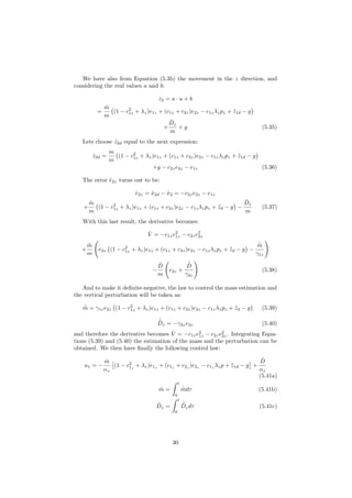
Figure 5.1: Example
two perturbations. In the Figure 5.1 an example of test for θ with a nominal
commanded value of 0.16 rad. The two perturbations are clearly visible at
t = 10 and 30 seconds. The nominal commanded values will be:
θcn
= [
π
4
,
3π
20
,
π
20
, −
π
20
, −
3π
20
, −
π
4
]
ψcn
= [π,
3π
5
,
π
5
, −
π
5
, −
3π
5
, −π]
For every test, three parameters will be measured. First, the quadratic error
of the overall simulation divided by the nominal commanded value, averaged
for the 6 tests:
Eθ =
1
6
6
i=1
(˜eθi + ˜eφi )
Eψ =
1
6
6
i=1
˜eψi
where the subscript i indicates the number of test and the squared errors are
defined as:
˜eθi =
1
θcni
tmax
0
(θ − θci
)
2
dt
˜eφi
=
1
θcni
tmax
0
(φ − φci
)
2
dt
˜eψi
=
1
ψcni
tmax
0
(ψ − ψci
)
2
dt
Secondly, the effort of the controller will be measured as well, being it defied
34](https://image.slidesharecdn.com/520123f2-eb82-4c72-acd5-0cf972ce5fd0-150625092845-lva1-app6892/85/Control-of-a-Quadcopter-36-320.jpg)
![Selection
Given a fitting value fm
for every member, the roulette wheel method will be
used to create the matting pool, which will be composed by a number of pairs
equal to the size of the population (Np = 30). These pairs will be chosen
from the previous generation randomly, taking into account a probability which
depends on the fitting value ˆfm
as follows:
Pm
=
fm
Np
i=1
fi
(5.54)
One parent will not be allowed to be matched with itself and the same pair
in the matting pool will be avoid either. It must be pointed out, that there will
be two independent matting pool, one for the θ variable and another one for ψ.
Recombination
For every pair of parents from the matting pool (recall that there are two), and
for every parameter of the solution, one will be taken randomly from one parent
to form the next generation. We will then obtain Np new solutions after the
recombination.
Although this method was the one used in [21], the new material which is
introduced in the generation is very small, since the recombination only takes
the material from one of the parents. One realizes after some simulations that
the complete generation tends to converge to a few different members.
Another recombination is proposed, which consists of making an weighted
average of both parents:
κoff = r · κ1 + (1 − r) · κ2 (5.55)
where κi is the parameter of the parent i and r is a random number between
0 and 1. This new method produces generations with members much more
different between them.
Mutation
For every parameter, there will be a probability of Pmut = 1/Np to be mutated;
this value is often taken so statistically is ensured, that in every generation there
will be at least one mutation in every parameter. If the mutation takes place,
it will happen as follows:
κ = κ + sign(0.5 − r1) ·
κmax
2
· r2 (5.56)
where r1 and r2 are two random number. If κ turns out to be negative, the
previous equation will be again calculated with new random parameters until it
becomes positive.
Next generation
The next generation will be made up with the best Np members of the previous
generation and the offspring generated from them.
36](https://image.slidesharecdn.com/520123f2-eb82-4c72-acd5-0cf972ce5fd0-150625092845-lva1-app6892/85/Control-of-a-Quadcopter-38-320.jpg)
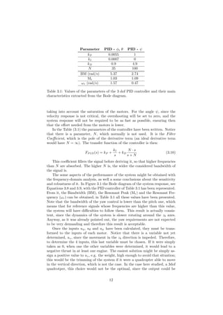
![Config. c1 c2 λ eλlim
E σ kb f
θ,φ
1 24.1 2.92 2.73 0.10 0.194 9.68 0.167 1
2 6.30 4.43 4.80 0.01 0.210 3.68 0.167 0.985
3 15.9 2.59 0.78 0.06 0.235 4.64 0.167 0.949
4 4.74 4.99 0.31 0.22 0.250 2.25 0.167 0.948
ψ
1 2.92 0.058 0.036 0.087 4.23 9.46 0.167 1
2 3.31 0.058 0.036 0.192 4.38 10.55 0 0.966
3 3.92 0.007 0.267 0.182 4.55 12.9 0.167 0.915
4 3.44 0.176 0.072 0.242 3.67 15.9 0 0.910
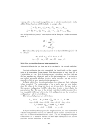
Table 5.1: Parameters of the best 4 configurations found by the genetic algo-
rithm, with their quadratic error E, effort σ and kickback measurement kb.
The above configuration will be run a maximum of 50 generations, being
stopped if in 5 generations in a row, there is not an improvement in the best
member of a 5%. Four different simulations will be carried out, two with the
recombination proposed in [21] and two more with the recombination based on
the weighted average of the two parents.
In the Table 3.1 the parameters of the four best configurations found by the
genetic algorithm for the θ/φ and for the ψ controller have been presented. Also
the values of the quadratic error E, the effort σ and the kickback number kb
haven also written, with the relative fitting value f. Note that configuration are
ordered so that the Configuration 1 is the best and the 4 is the worst.
The solutions for the controller of θ and φ are quite different between them,
although the final result is very similar. The configuration 1 has a very high c1
value so the effort is much higher than in the other configurations. Note that
for the four configurations there is at least a kickback in one of the 6 test, being
the kb = 1/6 = 0.167. On the other hand, the parameters for the ψ controller
are more similar between them, although the results are not.
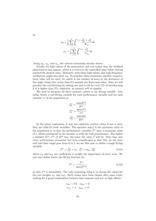
In the Figure 5.2 the time response of both controllers, with their four config-
urations, have been represented for an nominal input of θcn = 0.3 and ψcn = 1
rad. In the case of the pitch angle, see Figure 5.2a, configurations 1 and 2 are
very similar and the only clearly visible difference is that in presence of a pertur-
bation, configuration 1 returns to the reference value faster and therefore, the
error is lower, see Table 5.1. However, configuration 1 needs a way higher effort
and the likelihood of that the kickback shows up is also higher. Therefore, con-
figuration 2 will be chosen. On the other hand, for the angle ψ, Figure 5.2b, it
can be seen that configuration 4 is the best results in terms of velocity response
and error and it has not overshooting; however, it requires much more effort and
since the yaw control is not a relevant nor critical operation, it could prevent
the θ and φ controller to fulfill their duties in the best possible way. Because of
this, configuration 4 has been discarded and configuration 1 has been chosen,
which still has a fast response with a slight overshooting, but it requires less
control effort.
The parameters of the controllers chosen, with their main response charac-
teristics, have been presented in Table 5.2. The percentage of overshooting, the
delay time td, the rise time, tr and the settling time ts, all in seconds, have been
calculated having as a reference response the one shown in Figure 5.2.
37](https://image.slidesharecdn.com/520123f2-eb82-4c72-acd5-0cf972ce5fd0-150625092845-lva1-app6892/85/Control-of-a-Quadcopter-39-320.jpg)
![time [s]
0 5 10 15 20 25 30 35 40
θ[rad]
-0.05
0
0.05
0.1
0.15
0.2
0.25
0.3
0.35
0.4
Pitch angle θcn
=0.3
θc
Conf. 1
Conf. 2
Conf. 3
Conf. 4
(a) Time response of the 4 best
configurations of the θ and φ con-
troller.
time [s]
0 5 10 15 20 25 30 35 40
ψ[rad]
-0.2
0
0.2
0.4
0.6
0.8
1
1.2
Yaw angle ψcn
=1
ψc
Conf. 1
Conf. 2
Conf. 3
Conf. 4
(b) Time response of the 4 best
configurations of the ψ controller.
Figure 5.2: Time response of the controller with the best 4 configurations found,
see Table 5.1.
c1 c2 λ eλlim
maxover (%) td tr ts
θ,φ 6.30 4.43 4.80 0.01 - 0.27 0.42 0.82
ψ 2.92 0.058 0.036 0.087 2.8 1.88 4.03 5.68
Table 5.2: Values of the parameters of the controllers chosen, and their main
response characteristics of Figure 5.2.
38](https://image.slidesharecdn.com/520123f2-eb82-4c72-acd5-0cf972ce5fd0-150625092845-lva1-app6892/85/Control-of-a-Quadcopter-40-320.jpg)
![5.4.3 Position Controller
In the case of the position controller, there are more parameters to be deter-
mined. Also, there are more elements involved in the movement; not only a
position must be reached, but also the perturbation ˆD and the mass ˆm must be
estimated by different tests. As done with the attitude controller, the following
elements of the GA will be taken into consideration.
Initial population
The initial population will be taken randomly between a range of values, deter-
mined after some trials:
c1x,y
∈ [0, 5] λx,y ∈ [0, 2] ex,y
λlim
∈ [0, 0.1] kx,y ∈ [0, 5]
γx,y ∈ [0, 1] β1x,y ∈ [0, 2] β2x,y ∈ [0, 0.5] β3x,y ∈ [0, 5]
λz ∈ [0, 0.5] ez
λlim
∈ [0, 1] γ1z ∈ [0, 0.1]
γ2z ∈ [0, 0.1] c1z ∈ [0, 0.5] c2z ∈ [0, 2]
We will use again Np = 30 members. Since this controller is specially com-
plicated to be tuned, its likely that the first generations are made up with very
bad solutions. Therefore, 5 solutions with good performance will be included in
the initial population.
Representation
Again, the parameters will be represented as real numbers.
Evaluation
The performance of the controller of the x and y direction will be tested by
commanding different positions in the x direction, keeping altitude and position
along y direction. Also, different perturbation forces will be applied to the
quadcopter. The complete sequence of action to test the horizontal position
controller is:
1. Wait 2 second to stabilize the quadcopter in the z direction.
2. Go forward 1 m.
3. Go backward 2 m.
4. Go forward 7 m.
5. Go backward 13 m.
6. Go forward 23 m.
7. Go backward 33 m.
8. Go forward 10 m. back to the initial position.
9. Apply a perturbation force of 1 N.
10. Apply a perturbation force of 2 N.
39](https://image.slidesharecdn.com/520123f2-eb82-4c72-acd5-0cf972ce5fd0-150625092845-lva1-app6892/85/Control-of-a-Quadcopter-41-320.jpg)

![time [s]
0 20 40 60 80 100 120 140 160
X[m]
-10
-8
-6
-4
-2
0
2
4
6
8
10
Xr
X
(a) Movement in the xb direction.
time [s]
0 20 40 60 80 100 120 140 160ˆDx[N]
-3
-2
-1
0
1
2
3
Dx
ˆDx
(b) Estimation of the perturbation
Dx.
time [s]
0 20 40 60 80 100 120 140 160
Z[m]
-26
-24
-22
-20
-18
-16
-14
-12
-10
Zr
Z
(c) Movement in the zb direction.
time [s]
0 20 40 60 80 100 120 140 160
ˆDz[N]
-5
-4
-3
-2
-1
0
1
2
3
4
5
Dz
ˆDz
(d) Estimation of the perturba-
tion Dx.
time [s]
0 5 10 15 20 25 30
ˆm[kg]
1
1.1
1.2
1.3
1.4
1.5
1.6
1.7
1.8
m
ˆmz
(e) Estimation of the mass m.
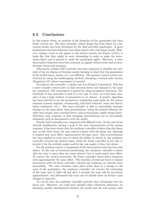
Figure 5.3: Result of the tests with configuration 3 for the controller in the xb
and yb direction and controller 1 in the zb direction.
44](https://image.slidesharecdn.com/520123f2-eb82-4c72-acd5-0cf972ce5fd0-150625092845-lva1-app6892/85/Control-of-a-Quadcopter-46-320.jpg)
![Characteristic x, y z
maxover (%) 6 -
td(s) 1.05 0.81
tr 1.52 2.14
ts 3.42 3.28
Table 5.4: Time characteristics of the two nonlinear controllers of the horizontal
and vertical positioning, with reference values x = 1 m and z = −1 m.
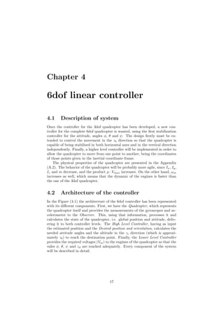
actual values. The controller is able to absorb firstly the excess of mass in the
first seconds, and afterwards the disturbances on every axes.
In Figure 5.4b the disturbances on the quadcopter and their estimation have
been represented. The three estimation remain close to the zero value until the
perturbations take place at 45, 65 and 85 s. The estimated values converge
approximately to the real values; although the approximation is not perfect, the
controller absorbs the perturbation, as can be seen in Figure 5.4a.
Finally, in Figure 5.4c the mass estimation and its real value has been shown.
Within 6 seconds, the algorithm estimates perfectly the real mass of the quad-
copter; afterwards, the mass estimation is disable and the final value used from
then on. The take off of the quadcopter delays the convergence of the estimation;
if we had considered that the quadcopter was already hovering, the convergence
would have taken place in less than 2 s. Once the mass has been estimated, its
value it passed to the x and y controller, see Equation 5.2; the update of the
value improves remarkably the performance of the position control, specially
when absorbing external perturbations.
It must be remark that the result here achieve seem to be better than those
obtained in [9]. Of course the quadcopter model is different and the final values
of the parameters are not specified, but the results present overshooting, high
oscillations and irregularities. The method there used to choose the parameters
is not specified.
45](https://image.slidesharecdn.com/520123f2-eb82-4c72-acd5-0cf972ce5fd0-150625092845-lva1-app6892/85/Control-of-a-Quadcopter-47-320.jpg)
![time [s]
0 20 40 60 80 100 120
Position[m]
-1.5
-1
-0.5
0
0.5
1
1.5
X
Y
Z
(a) Position of the quadcopter.
time [s]
0 20 40 60 80 100 120
ˆD
-3
-2
-1
0
1
2
3
ˆDx
ˆDx
ˆDx
(b) Estimation of the perturba-
tions.
time [s]
0 1 2 3 4 5 6
ˆm
1.4
1.45
1.5
1.55
1.6
1.65
1.7
1.75
1.8
(c) Estimation of the mass m dur-
ing the first 5 seconds.
Figure 5.4: Test with the final configuration of the controller, similar to the one
in Figure 4.4a, but with a change of +0.3 kg in the mass and perturbations in
the three axes.
46](https://image.slidesharecdn.com/520123f2-eb82-4c72-acd5-0cf972ce5fd0-150625092845-lva1-app6892/85/Control-of-a-Quadcopter-48-320.jpg)

![time [s]
0 1 2 3 4 5
θ[rad]
0
0.1
0.2
0.3
0.4
0.5
0.6
0.7
Reference
Lineal
Non-lineal
(a) Pitch angle response.
time [s]
0 5 10 15 20
ψ[rad]
0
0.2
0.4
0.6
0.8
1
1.2
Reference
Lineal
Non-lineal
(b) Yaw angle response.
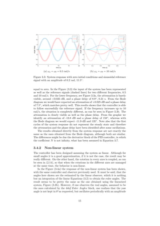
Figure 6.1: System response comparison between the linear controller, in red,
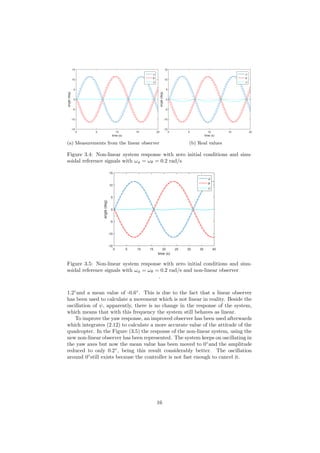
and the nonlinear controller, in red.
a perturbation, the controller does not succeed on coming back to the desired
value. Furthermore, if we take a look on the needed effort, defined by Equation
5.49, we have:
σθlinear
= 0.40
σθnonlinear
= 0.24
the effort is much higher in the linear controller, so the nonlinear controller is
visibly better.
The case of the ψ controller is different. As said, the PID controller con-
verges faster to the reference signal, but it needs more time to recover after the
perturbation. Also, the efforts are:
σψlinear
= 2.86
σψnonlinear
= 0.70
The effort needed by the linear controller is 40 times higher than the one
needed by the nonlinear controller. If we needed the yaw response to be faster,
we could configure the parameter selection algorithm so that the error is more
important, by reducing the weight of the effort.
6.2 Position controllers
To compare both high level controller, we will design 5 different tests. First,
the system response reaching the positions x = 1 m and z = −1 m will be
analyzed independently. Another two experiments will be carried out, in which
an external force in the x and −z will be applied, while the quadcopter tries to
remain in the initial position. Finally, an additional mass will be added and the
altitude will be checked to see if the controllers are able to keep it. In Figure
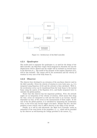
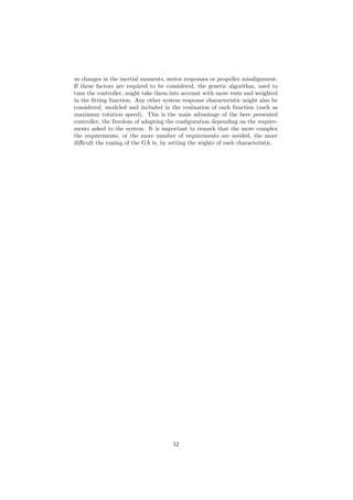
6.2 all the tests’ results have been presented.
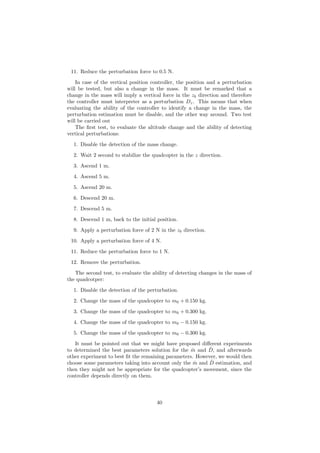
In Figure 6.2a the system response with both controllers have been shown,
when commanded with a reference signal x =1 m. The nonlinear controller
turns out to be faster, having a small overshooting. On the other hand, in Figure
48](https://image.slidesharecdn.com/520123f2-eb82-4c72-acd5-0cf972ce5fd0-150625092845-lva1-app6892/85/Control-of-a-Quadcopter-50-320.jpg)
![6.2b the movement in the zb axes can be seen, being initially the quadcopter
grounded and taking off to an altitude of z = −1 m. In this case, the linear
controller is faster than the nonlinear one. The time domain characteristics of
both controllers, in both axes are the following:
Controller maxover (%) td(s) tr ts
x,y
Linear 0 1.58 3.72 5.51
Nonlinear 6 1.05 1.52 3.42
z
Linear 0 0.41 1.00 1.55
Nonlinear 0 0.81 2.14 3.28
It should be remarked that the PID controller in the zb is 2 times faster than
the nonlinear controller, which is an important advantage. The effort turns out
to be:
σzlinear
= 2081
σznonlinear
= 1904
Both controllers need almost the same effort. If we define now the effort to
reach a position in the x direction as:
σx = σθ =
t
0
uθ · dt (6.4)
the effort of both controller to reach the [1,0] position are:
σxlinear
= 0.104
σxnonlinear
= 2.053
The nonlinear controller need 20 times more effort to reach the desired po-
sition.
In Figure 6.2c, an external force of 2 N in the x direction has been applied,
being shown the position along this axis. The lineal controller is not able to
absorb the force and come back to the initial position; only after 25 s, when the
quadcopter reaches x = 10.5 m, the error term of the backstepping controller
in high enough to counteract the perturbation and the quadcopter starts slowly
returning to the initial position (not shown in the figure). On the other hand,
the nonlinear controller absorbs the perturbation in within 9 s, keeping the
quadcopter closer than 30 cm from the required position.
The situation when applying a vertical force Dz is similar, but the linear
controller is not able to return to the initial position and only keeps the altitude
at z = −1.6 m (note that the direction of the force is zb). On the contrary, the
nonlinear controller returns slowly to the reference altitude, and also avoids the
quadcopter to increase its altitude more than 0.25 m.
Finally, if an additional mass is added to the quacopter, the nonlinear con-
troller estimates it successfully and returns to the desired altitude in less than
2 s, as can be seen in Figure 6.2e. As it happened when adding an external ver-
tical force, the linear controller can not absorb it and the quadcopter decreases
the altitude because of the additional mass down to 0.42 cm.
49](https://image.slidesharecdn.com/520123f2-eb82-4c72-acd5-0cf972ce5fd0-150625092845-lva1-app6892/85/Control-of-a-Quadcopter-51-320.jpg)
![time [s]
0 2 4 6 8 10
X[m]
0
0.2
0.4
0.6
0.8
1
1.2
Reference
Lineal
Non-lineal
(a) Movement in the x direction.
time [s]
0 2 4 6 8 10
Z[m]
-1
-0.8
-0.6
-0.4
-0.2
0
0.2
Reference
Lineal
Non-lineal
(b) Movement in the zb direction.
time [s]
0 2 4 6 8 10
X[m]
0
1
2
3
4
5
6
7
Reference
Lineal
Non-lineal
(c) Movement in the x direction
with non zero Dx.
time [s]
0 2 4 6 8 10
Z[m]
-1.6
-1.5
-1.4
-1.3
-1.2
-1.1
-1
-0.9
Reference
Lineal
Non-lineal
(d) Movement in the zb direction
with non zero Dz.
time [s]
0 2 4 6 8 10
Z[m]
-1.1
-1
-0.9
-0.8
-0.7
-0.6
-0.5
-0.4
Reference
Lineal
Non-lineal
(e) Movement in the zb direction
with an additional mass.
Figure 6.2: Comparison of the system position response in the five different
cases considered.
50](https://image.slidesharecdn.com/520123f2-eb82-4c72-acd5-0cf972ce5fd0-150625092845-lva1-app6892/85/Control-of-a-Quadcopter-52-320.jpg)
![Bibliography
[1] Adamy, J. (2005). Implicit Lyapunov functions and isochrones of linear sys-
tems. IEEE Transactions on Automatic Control, 50(6), 874-879.
[2] Argentim, L. M., Rezende, W. C., Santos, P. E., & Aguiar, R. A. (2013,
May). PID, LQR and LQR-PID on a quadcopter platform. In Informatics,
Electronics & Vision (ICIEV), 2013 International Conference on (pp. 1-6).
IEEE.
[3] Bai, Y., Liu, H., Shi, Z., & Zhong, Y. (2012, July). Robust control of quadro-
tor unmanned air vehicles. In Control Conference (CCC), 2012 31st Chinese
(pp. 4462-4467). IEEE.
[4] Bouabdallah, S., & Siegwart, R. (2005, April). Backstepping and sliding-
mode techniques applied to an indoor micro quadrotor. In Robotics and
Automation, 2005. ICRA 2005. Proceedings of the 2005 IEEE International
Conference on (pp. 2247-2252). IEEE.
[5] Bouffard, P. (2012). On-board Model Predictive Control of a Quadrotor He-
licopter: Design, Implementation, and Experiments (No. UCB/EECS-2012-
241). CALIFORNIA UNIV BERKELEY DEPT OF COMPUTER SCI-
ENCES.
[6] Chen, B. S., Cheng, Y. M., & Lee, C. H. (1995). A genetic approach to
mixed H2/H∞ optimal PID control. Control Systems, IEEE, 15(5), 51-60.
[7] Diao, C., Xian, B., Yin, Q., Zeng, W., Li, H., & Yang, Y. (2011, May). A
nonlinear adaptive control approach for quadrotor UAVs. In Control Con-
ference (ASCC), 2011 8th Asian (pp. 223-228). IEEE.
[8] Dierks, T., & Jagannathan, S. (2010). Output feedback control of a quadro-
tor UAV using neural networks. Neural Networks, IEEE Transactions on,
21(1), 50-66.
[9] Fang, Z., & Gao, W. (2011, July). Adaptive integral backstepping control of
a micro-quadrotor. In Intelligent Control and Information Processing (ICI-
CIP), 2011 2nd International Conference on (Vol. 2, pp. 910-915). IEEE.
[10] Fatan, M., Sefidgari, B. L., & Barenji, A. V. (2013, August). An adap-
tive neuro PID for controlling the altitude of quadcopter robot. In Methods
and Models in Automation and Robotics (MMAR), 2013 18th International
Conference on (pp. 662-665). IEEE.
55](https://image.slidesharecdn.com/520123f2-eb82-4c72-acd5-0cf972ce5fd0-150625092845-lva1-app6892/85/Control-of-a-Quadcopter-57-320.jpg)
![[11] Fleming, P. J., & Purshouse, R. C. (2002). Evolutionary algorithms in
control systems engineering: a survey. Control engineering practice, 10(11),
1223-1241.
[12] Giagkiozis, I., & Fleming, P. J. (2015). Methods for multi-objective opti-
mization: An analysis. Information Sciences, 293, 338-350.
[13] Hably, A., Kendoul, F., Marchand, N., & Castillo, P. (2006). Further results
on global stabilization of the PVTOL aircraft. Positive Systems, 303-310.
[14] Hoffmann, G. M., Huang, H., Waslander, S. L., & Tomlin, C. J. (2007, Au-
gust). Quadrotor helicopter flight dynamics and control: Theory and exper-
iment. In Proc. of the AIAA Guidance, Navigation, and Control Conference
(Vol. 2).
[15] Huo, X., Huo, M., & Karimi, H. R. (2014). Attitude stabilization control of
a quadrotor UAV by using backstepping approach. Mathematical Problems
in Engineering, 2014.
[16] Lee, K. U., Kim, H. S., Park, J. B., & Choi, Y. H. (2012, October). Hovering
control of a quadrotor. In Control, Automation and Systems (ICCAS), 2012
12th International Conference on (pp. 162-167). IEEE.
[17] Li, J., & Li, Y. (2011, August). Dynamic analysis and PID control for
a quadrotor. In Mechatronics and Automation (ICMA), 2011 International
Conference on (pp. 573-578). IEEE.
[18] NG TZE HUI, T. H. O. M. A. S. (2007). Design optimization of small-scale
unmanned air vehicles (Doctoral dissertation).
[19] Palunko, I., & Fierro, R. (2011, August). Adaptive control of a quadrotor
with dynamic changes in the center of gravity. In Proceedings 18th IFAC
World Congress (Vol. 18, No. 1, pp. 2626-2631).
[20] Santos, M., Lopez, V., & Morata, F. (2010, November). Intelligent fuzzy
controller of a quadrotor. In Intelligent Systems and Knowledge Engineering
(ISKE), 2010 International Conference on (pp. 141-146). IEEE.
[21] Shen, J. C. (2002). New tuning method for PID controller. ISA transactions,
41(4), 473-484.
[22] Sutarto, H. Y., Budiyono, A., Joelianto, E., & Hiong, G. T. (2006, Decem-
ber). Switched linear control of a model helicopter. In Control, Automation,
Robotics and Vision, 2006. ICARCV’06. 9th International Conference on
(pp.1-8). IEEE.
[23] Yang, Z., & Pedersen, G. (2006, October). Automatic tuning of PID con-
troller for a 1-D levitation system using a genetic algorithm-a real case study.
In Computer Aided Control System Design, 2006 IEEE International Con-
ference on Control Applications, 2006 IEEE International Symposium on
Intelligent Control, 2006 IEEE (pp. 3098-3103). IEEE.
[24] Zulu, A., & John, S. (2014). A Review of Control Algorithms for Au-
tonomous Quadrotors. Open Journal of Applied Sciences, 4(14), 547.
56](https://image.slidesharecdn.com/520123f2-eb82-4c72-acd5-0cf972ce5fd0-150625092845-lva1-app6892/85/Control-of-a-Quadcopter-58-320.jpg)