Download as PDF, PPTX
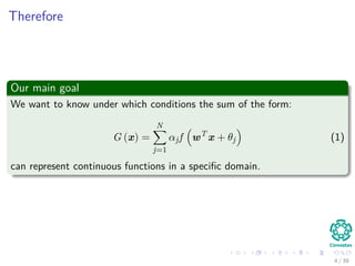
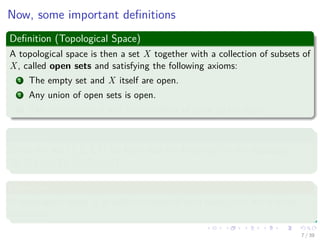
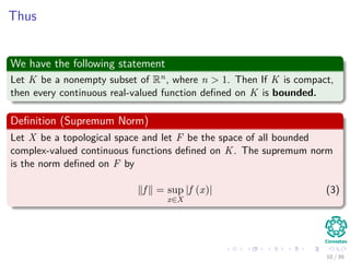
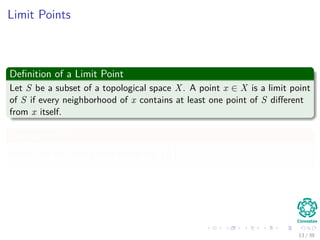
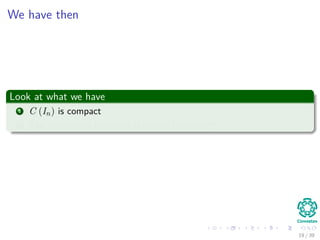
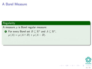
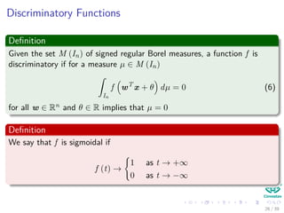
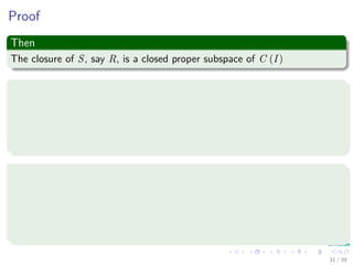
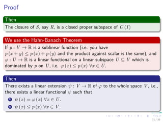
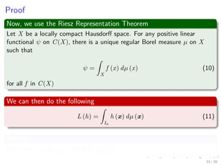
![Setup of the problem
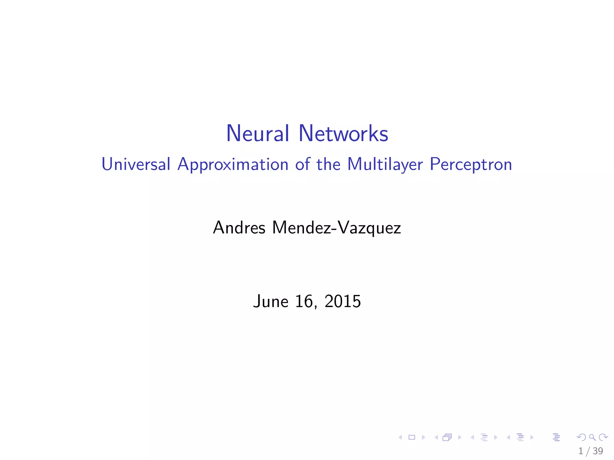
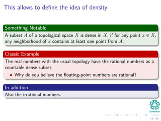
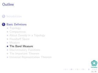
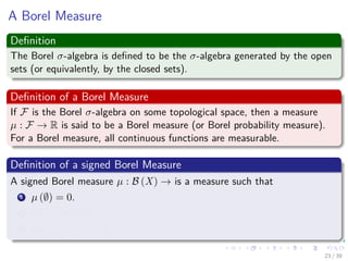
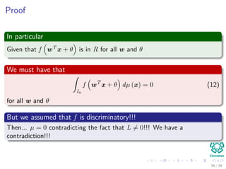
Definition of In
It is an n-dimensional unit cube [0, 1]n
In addition, we have the following set of functions
C (In) = {f : In → R|f is a continous function} (2)
5 / 39](https://image.slidesharecdn.com/07-151212040422/85/16-Machine-Learning-Universal-Approximation-Multilayer-Perceptron-6-320.jpg)
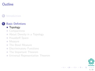
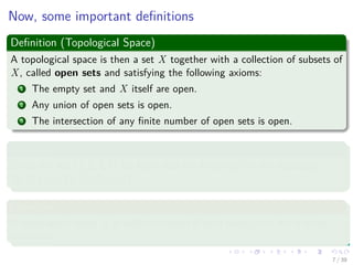
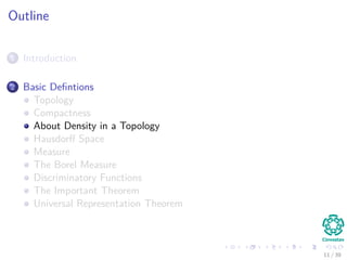
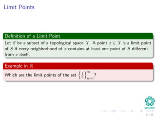
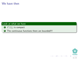
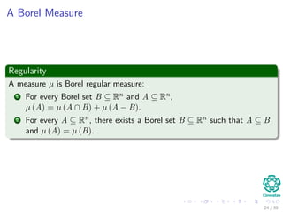
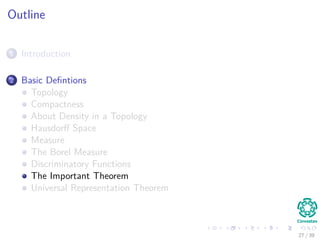
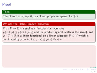
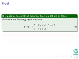
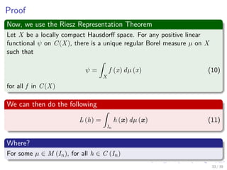
![Setup of the problem
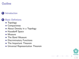
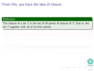
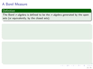
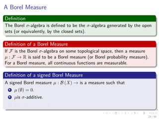
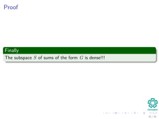
Definition of In
It is an n-dimensional unit cube [0, 1]n
In addition, we have the following set of functions
C (In) = {f : In → R|f is a continous function} (2)
5 / 39](https://image.slidesharecdn.com/07-151212040422/85/16-Machine-Learning-Universal-Approximation-Multilayer-Perceptron-7-320.jpg)
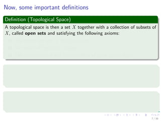
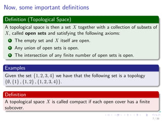
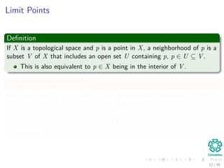
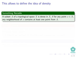

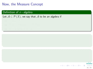
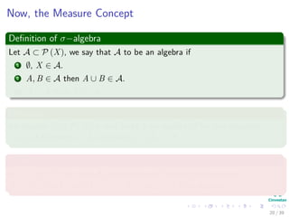
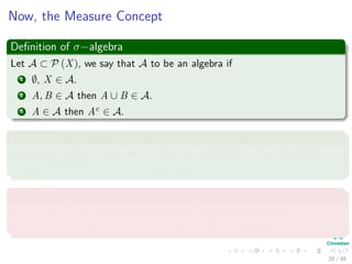
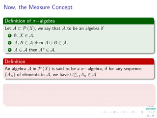
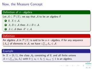
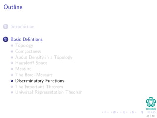
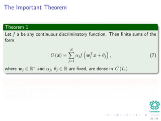
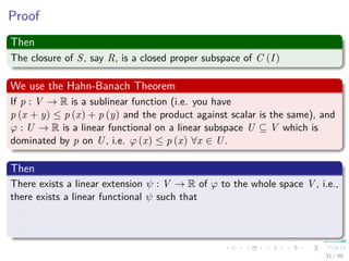
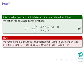
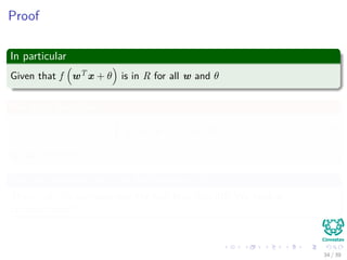
![Now, the Measure Concept
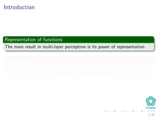
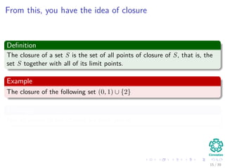
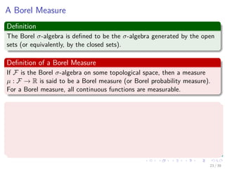
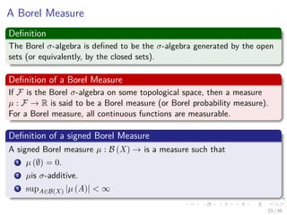
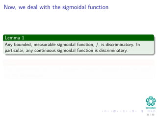
Definition of additivity
Let µ : A → [0, +∞] be such that µ (∅) = 0, we say that µ is σ−additive
if for any {Ai}i∈I ⊂ A (Where I can be finite of infinite countable) of
mutually disjoint sets such that ∪i∈I Ai ∈ A, we have that
µ (∪i∈I Ai) =
i∈I
µ (Ai) (5)
Definition of Measurability
Let A be a σ−algebra of subsets of X, we say that the [air (X, A) is a
measurable space where a σ−additive function µ : A → [0, +∞] is called a
measure on (X, A).
21 / 39](https://image.slidesharecdn.com/07-151212040422/85/16-Machine-Learning-Universal-Approximation-Multilayer-Perceptron-44-320.jpg)
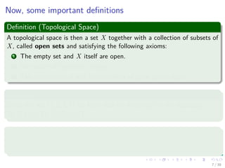
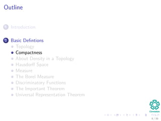
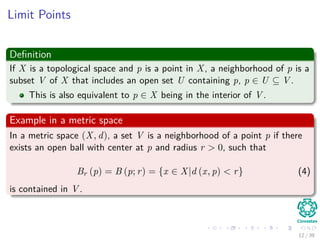
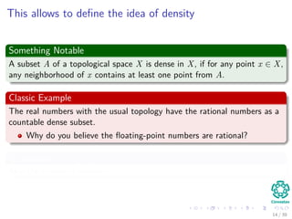
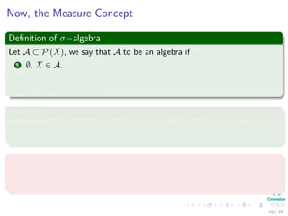
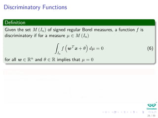
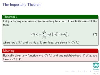
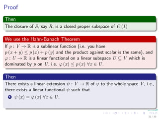
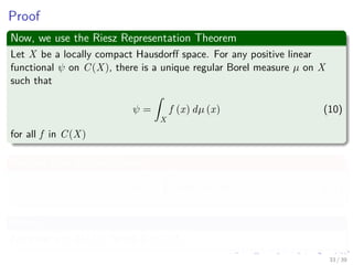
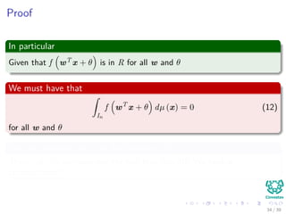
![Now, the Measure Concept
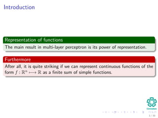
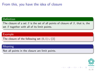
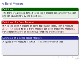
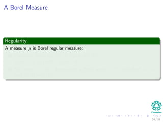
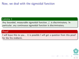
Definition of additivity
Let µ : A → [0, +∞] be such that µ (∅) = 0, we say that µ is σ−additive
if for any {Ai}i∈I ⊂ A (Where I can be finite of infinite countable) of
mutually disjoint sets such that ∪i∈I Ai ∈ A, we have that
µ (∪i∈I Ai) =
i∈I
µ (Ai) (5)
Definition of Measurability
Let A be a σ−algebra of subsets of X, we say that the [air (X, A) is a
measurable space where a σ−additive function µ : A → [0, +∞] is called a
measure on (X, A).
21 / 39](https://image.slidesharecdn.com/07-151212040422/85/16-Machine-Learning-Universal-Approximation-Multilayer-Perceptron-45-320.jpg)

The document discusses the universal approximation theorem for multilayer perceptrons, focusing on the conditions under which continuous functions can be represented as finite sums of simpler functions. It elaborates on various concepts in topology, such as compactness, limit points, dense subsets, and the properties of Hausdorff spaces, culminating in the exploration of measure theory and sigma-algebras. The main objective is to assess the representation capabilities of neural networks in approximating continuous functions defined on compact subsets of R^n.


![Competitive Learning [Deep Learning And Nueral Networks].pptx](https://cdn.slidesharecdn.com/ss_thumbnails/competitivelearning-240211053020-bc9a8437-thumbnail.jpg?width=640&height=640&fit=bounds)