This document provides an overview of preliminary topological concepts needed for applied mathematics. It defines topological spaces and metric spaces, and introduces key topological notions like open and closed sets, bases for topologies, convergence of sequences, accumulation points, interior and closure of sets, and dense sets. Metric spaces are shown to induce a natural topological structure, though not all topologies come from a metric. Examples are provided to illustrate various definitions and properties.

1. Methods of Applied Mathematics
Todd Arbogast and Jerry L. Bona
Department of Mathematics, and
Institute for Computational Engineering and Sciences
The University of Texas at Austin
Copyright 1999–2001, 2004–2005, 2007–2008 (corrected version)
by T. Arbogast and J. Bona.

3. Contents
Chapter 1. Preliminaries 5
1.1. Elementary Topology 5
1.2. Lebesgue Measure and Integration 13
1.3. Exercises 23
Chapter 2. Normed Linear Spaces and Banach Spaces 27
2.1. Basic Concepts and Definitions. 27
2.2. Some Important Examples 34
2.3. Hahn-Banach Theorems 43
2.4. Applications of Hahn-Banach 48
2.5. The Embedding of X into its Double Dual X∗∗ 52
2.6. The Open Mapping Theorem 53
2.7. Uniform Boundedness Principle 57
2.8. Compactness and Weak Convergence in a NLS 58
2.9. The Dual of an Operator 63
2.10. Exercises 66
Chapter 3. Hilbert Spaces 73
3.1. Basic Properties of Inner-Products 73
3.2. Best Approximation and Orthogonal Projections 75
3.3. The Dual Space 78
3.4. Orthonormal Subsets 79
3.5. Weak Convergence in a Hilbert Space 86
3.6. Exercises 87
Chapter 4. Spectral Theory and Compact Operators 89
4.1. Definitions of the Resolvent and Spectrum 90
4.2. Basic Spectral Theory in Banach Spaces 91
4.3. Compact Operators on a Banach Space 93
4.4. Bounded Self-Adjoint Linear Operators on a Hilbert Space 99
4.5. Compact Self-Adjoint Operators on a Hilbert Space 104
4.6. The Ascoli-Arzelà Theorem 107
4.7. Sturm Liouville Theory 109
4.8. Exercises 122
Chapter 5. Distributions 125
5.1. The Notion of Generalized Functions 125
5.2. Test Functions 127
5.3. Distributions 129
5.4. Operations with Distributions 133
3

4. 4 CONTENTS
5.5. Convergence of Distributions and Approximations to the Identity 138
5.6. Some Applications to Linear Differential Equations 140
5.7. Local Structure of D0 148
5.8. Exercises 148
Chapter 6. The Fourier Transform 151
6.1. The L1(Rd) Theory 153
6.2. The Schwartz Space Theory 157
6.3. The L2(Rd) Theory 162
6.4. The S0 Theory 164
6.5. Some Applications 170
6.6. Exercises 172
Chapter 7. Sobolev Spaces 177
7.1. Definitions and Basic Properties 177
7.2. Extensions from Ω to Rd 181
7.3. The Sobolev Imbedding Theorem 185
7.4. Compactness 191
7.5. The Hs Sobolev Spaces 193
7.6. A Trace Theorem 198
7.7. The Ws,p(Ω) Sobolev Spaces 203
7.8. Exercises 204
Chapter 8. Boundary Value Problems 207
8.1. Second Order Elliptic Partial Differential Equations 207
8.2. A Variational Problem and Minimization of Energy 210
8.3. The Closed Range Theorem and Operators Bounded Below 213
8.4. The Lax-Milgram Theorem 215
8.5. Application to Second Order Elliptic Equations 219
8.6. Galerkin Approximations 224
8.7. Green’s Functions 226
8.8. Exercises 229
Chapter 9. Differential Calculus in Banach Spaces and the Calculus of Variations 233
9.1. Differentiation 233
9.2. Fixed Points and Contractive Maps 241
9.3. Nonlinear Equations 245
9.4. Higher Derivatives 252
9.5. Extrema 256
9.6. The Euler-Lagrange Equations 259
9.7. Constrained Extrema and Lagrange Multipliers 265
9.8. Lower Semi-Continuity and Existence of Minima 269
9.9. Exercises 273
Bibliography 279

5. CHAPTER 1
Preliminaries
We discuss in this Chapter some of the pertinent aspects of topology and measure theory
that are needed in the course of the rest of the book. We treat this material as background, and
well prepared students may wish to skip either of both topics.
1.1. Elementary Topology
In applied mathematics, we are often faced with analyzing mathematical structures as they
might relate to real-world phenomena. In applying mathematics, real phenomena or objects are
conceptualized as abstract mathematical objects. Collections of such objects are called sets.
The objects in a set of interest may also be related to each other; that is, there is some structure
on the set. We call such structured sets spaces.
Examples. (1) A vector space (algebraic structure).
(2) The set of integers Z (number theoretical structure or arithmetic structure).
(3) The set of real numbers R or the set of complex numbers C (algebraic and topological
structure).
We start the discussion of spaces by putting forward sets of “points” on which we can talk about
the notions of convergence or limits and associated continuity of functions.
A simple example is a set X with a notion of distance between any two points of X. A
sequence {xn}∞
n=1 ⊂ X converges to x ∈ X if the distance from xn to x tends to 0 as n increases.
This definition relies on the following formal concept.
Definition. A metric or distance function on a set is a function d : X × X → R satisfying:
(1) (positivity) for any x, y ∈ X, d(x, y) ≥ 0, and d(x, y) = 0 if and only if x = y;
(2) (symmetry) for any x, y ∈ X, d(x, y) = d(y, x);
(3) (triangle inequality) for any x, y, z ∈ X, d(x, y) ≤ d(x, z) + d(z, y).
A metric space (X, d) is a set X together with an associated metric d : X × X → R.
Example. (Rd, | · |) is a metric space, where for x, y ∈ Rd, the distance from x to y is
|x − y| =
d
X
i=1
(xi − yi)2
1/2
.
It turns out that the notion of distance or metric is sometimes stronger than what actu-
ally appears in practice. The more fundamental concept upon which much of the mathematics
developed here rests, is that of limits. That is, there are important spaces arising in applied
mathematics that have well defined notions of limits, but these limiting processes are not com-
patible with any metric. We shall see such examples later; let it suffice for now to motivate a
weaker definition of limits.
5

6. 6 1. PRELIMINARIES
A sequence of points {xn}∞
n=1 can be thought of as converging to x if every “neighborhood” of
x contains all but finitely many of the xn, where a neighborhood is a subset of points containing
x that we think of as “close” to x. Such a structure is called a topology. It is formalized as
follows.
Definition. A topological space (X, T ) is a nonempty set X of points with a family T of
subsets, called open, with the properties:
(1) X ∈ T , ∅ ∈ T ;
(2) If ω1, ω2 ∈ T , then ω1 ∩ ω2 ∈ T ;
(3) If ωα ∈ T for all α in some index set I, then
S
α∈I ωα ∈ T .
The family T is called a topology for X. Given A ⊂ X, we say that A is closed if its complement
Ac = X A = {x ∈ X : x 6∈ A} is open.
Example. If X is any nonempty set, we can always define the two topologies:
(1) T1 = {∅, X}, called the trivial topology;
(2) T2 consisting of the collection of all subsets of X, called the discrete topology.
Proposition 1.1. The sets ∅ and X are both open and closed. Any finite intersection of
open sets is open. Any intersection of closed sets is closed. The union of any finite number of
closed sets is closed.
Proof. We need only show the last two statements, as the first two follow directly from the
definitions. Let Aα ⊂ X be closed for α ∈ I. Then one of deMorgan’s laws gives that
α∈I
Aα
c
=
[
α∈I
Ac
α is open.
Finally, if J ⊂ I is finite, the other deMorgan law gives
[
α∈J
Aα
c
=
α∈J
Ac
α is open.
It is often convenient to define a simpler collection of open sets that immediately generates
a topology.
Definition. Given a topological space (X, T ) and an x ∈ X, a base for the topology at x
is a collection Bx of open sets containing x such that for any open E 3 x, there is B ∈ Bx such
that
x ∈ B ⊂ E .
A base for the topology, B, is a collection of open sets that contains a base at x for all x ∈ X.
Proposition 1.2. A collection B of subsets of X is a base for a topology T if and only if
(1) each x ∈ X is contained in some B ∈ B and (2) if x ∈ B1 ∩ B2 for B1, B2 ∈ B, then there is
some B3 ∈ B such that x ∈ B3 ⊂ B1 ∩ B2. If (1) and (2) are valid, then
T = {E ⊂ X : E is a union of subsets in B} .
Proof. (⇒) Since X and B1 ∩ B2 are open, (1) and (2) follow from the definition of a base
at x.
(⇐) Let T be defined as above. Then ∅ ∈ T (the vacuous union), X ∈ T by (1), and
arbitrary unions of sets in T are again in T . It remains to show the intersection property. Let

7. 1.1. ELEMENTARY TOPOLOGY 7
E1, E2 ∈ T , and x ∈ E1 ∩ E2 (if E1 ∩ E2 = ∅, there is nothing to prove). Then there are sets
B1, B2 ∈ B such that
x ∈ B1 ⊂ E1 , x ∈ B2 ⊂ E2 ,
so
x ∈ B1 ∩ B2 ⊂ E1 ∩ E2 .
Now (2) gives B3 ∈ B such that
x ∈ B3 ⊂ E1 ∩ E2 .
Thus E1 ∩ E2 is a union of elements in B, and is thus in T .
We remark that instead of using open sets, one can consider neighborhoods of points x ∈ X,
which are sets N 3 x such that there is an open set E satisfying x ∈ E ⊂ N.
Theorem 1.3. If (X, d) is a metric space, then (X, T ) is a topological space, where a base
for the topology is given by
TB = {Br(x) : x ∈ X and r 0} ,
where
Br(x) = {y ∈ X : d(x, y) r}
is the ball of radius r about x.
Proof. Point (1) is clear. For (2), suppose x ∈ Br(y) ∩ Bs(z). Then x ∈ Bρ(x) ⊂ Br(y) ∩
Bs(z), where ρ = 1
2 min(r − d(x, y), s − d(x, z)) 0.
Thus metric spaces have a natural topological structure. However, not all topological spaces
are induced as above by a metric, so the class of topological spaces is genuinely richer.
Definition. Let (X, T ) be a topological space. The closure of A ⊂ X, denoted Ā, is the
intersection of all closed sets containing A:
Ā =
F closed
F⊇A
F .
Proposition 1.4. The set Ā is closed, and it is the smallest closed set containing A.
Proof. This follows by Proposition 1.1 and the definition.
Definition. The interior of A ⊂ X, denoted A◦, is the union of all open sets contained in
A:
A◦
=
[
E open
E⊂A
E .
Proposition 1.5. The set A◦ is open, and is the largest open set contained in A.
Proof. This also follows from Proposition 1.1 and the definition.
Proposition 1.6. It holds that A ⊂ Ā, ¯
Ā = Ā, A ⊂ B =⇒ Ā ⊂ B̄, A ∪ B = Ā ∪ B̄, and
A closed ⇔ A = Ā. Moreover, A ⊃ A◦, A◦◦ = A◦, A ⊂ B =⇒ A◦ ⊂ B◦, (A ∩ B)◦ = A◦ ∩ B◦,
and A open ⇔ A = A◦.
These results are left to the reader to prove.

8. 8 1. PRELIMINARIES
Proposition 1.7. It holds that (Ac)◦ = (Ā )c and (A◦)c = (Ac).
Proof. We have
x /
∈ ( Ā )c
⇔ x ∈ Ā ⇔ x ∈
F closed
F⊃A
F ⇔ x /
∈
F closed
F⊃A
F
c
⇔ x /
∈
[
Fc open
Fc⊂Ac
Fc
= (Ac
)◦
.
The second result is similar.
Definition. A point x ∈ X is an accumulation point of A ⊂ X if every open set containing
x intersects A {x}. Also, a point x ∈ A is an interior point of A if there is some open set E
such that
x ∈ E ⊂ A .
Finally, x ∈ A is an isolated point if there is an open set E 3 x such that E {x} ∩ A = ∅.
Proposition 1.8. For A ⊂ X, Ā is the union of the set of accumulation points of A and A
itself, and A0 is the union of the interior points of A.
Proof. Exercise.
Definition. A set A ⊂ X is dense in X if Ā = X.
Definition. The boundary of A ⊂ X, denoted ∂A, is
∂A = Ā ∩ Ac .
Proposition 1.9. If A ⊂ X, then ∂A is closed and
Ā = A◦
∪ ∂A , A◦
∩ ∂A = ∅ .
Moreover,
∂A = ∂Ac
= {x ∈ X : every open E 3 x intersects both A and Ac
} .
Proof. Exercise.
Definition. A sequence {xn}∞
n=1 ⊂ X converges to x ∈ X, or has limit x, if given any open
E 3 x, there is N 0 such that xn ∈ E for all n ≥ N (i.e., the entire tail of the sequence is
contained in E).
Proposition 1.10. If limn→∞ xn = x, then x is an accumulation point of {xn}∞
n=1, inter-
preted as a set.
Proof. Exercise.
We remark that if x is an accumulation point of {xn}∞
n=1, there may be no subsequence
{xnk
}∞
k=1 converging to x.
Example. Let X be the set of nonnegative integers, and a base TB = {{0, 1, . . . , i} for
each i ≥ 1}. Then {xn}∞
n=1 with xn = n has 0 as an accumulation point, but no subsequence
converges to 0.
If xn → x ∈ X and xn → y ∈ X, it is possible that x 6= y.
Example. Let X = {a, b} and T = {∅, {a}, {a, b}}. Then the sequence xn = a for all n
converges to both a and b.

9. 1.1. ELEMENTARY TOPOLOGY 9
Definition. A topological space (X, T ) is called Hausdorff if given distinct x, y ∈ X, there
are disjoint open sets E1 and E2 such that x ∈ E1 and y ∈ E2.
Proposition 1.11. If (X, T ) is Hausdorff, then every set consisting of a single point is
closed. Moreover, limits of sequences are unique.
Proof. Exercise.
Definition. A point x ∈ X is a strict limit point of A ⊂ X if there is a sequence {xn}∞
n=1 ⊂
A {x} such that limn→∞ xn = x.
Note that if x is an isolated point of X, then x /
∈ A◦, so ∂A 6= ∂(A◦) in general.
Metric spaces are less susceptible to pathology than general topological spaces. For example,
they are Hausdorff.
Proposition 1.12. If (X, d) is a metric space and A ⊂ X, then every x ∈ ∂A is either an
isolated point, or a strict limit point of A and Ac.
Proof. Exercise.
Proposition 1.13. If (X, d) is a metric space and {xn}∞
n=1 is a sequence in X, then xn → x
if and only if, given ε 0, there is N 0 such that
d(x, xn) ε ∀ n ≥ N .
That is, xn ∈ Bε(x) for all n ≥ N.
Proof. If xn → x, then the tail of the sequence is in every open set E 3 x. In particular,
this holds for the open sets Bε(x). Conversely, if E is any open set containing x, then the open
balls at x form a base for the topology, so there is some Bε(x) ⊂ E which contains the tail of
the sequence.
Proposition 1.14. Every metric space is Hausdorff.
Proof. Exercise.
Proposition 1.15. If (x, d) is a metric space and A ⊂ X has an accumulation point x,
Then there is some sequence {xn}∞
n=1 ⊂ A such that xn → x.
Proof. Given integer n ≥ 1, there is some xn ∈ B1/n(x), since x is an accumulation point.
Thus xn → x.
We avoid problems arising with limits in general topological spaces by the following definition
of continuity.
Definition. A mapping f of a topological space (X, T ) into a topological space (Y, S) is
continuous if the inverse image of every open set in Y is open in X.
This agrees with our notion of continuity on R.
We say that f is continuous at a point x ∈ X if given any open set E ⊂ Y containing f(x),
then f−1(E) contains an open set D containing x. That is,
x ∈ D and f(D) ⊂ E .
A map is continuous if and only if it is continuous at each point of X.
Proposition 1.16. If f : X → Y and g : Y → Z are continuous, then g ◦ f : X → Z is
continuous.

10. 10 1. PRELIMINARIES
Proof. Exercise.
Proposition 1.17. If f is continuous and xn → x, then f(xn) → f(x).
Proof. Exercise.
The converse of Proposition 1.17 is false in general. When the hypothesis xn → x always
implies f(xn) → f(x), we say that f is sequentially continuous.
Proposition 1.18. If f : X → Y is sequentially continuous, and if X is a metric space,
then f is continuous.
Proof. Let E ⊂ Y be open and A = f−1(E). We must show that A is open. Suppose not.
Then there is some x ∈ A such that Br(x) 6⊂ A for all r 0. Thus for rn = 1/n, n ≥ 1 an
integer, there is some xn ∈ Brn (x) ∩ Ac. Since xn → x, f(xn) → f(x) ∈ E. But f(xn) ∈ Ec
for all n, so f(x) is an accumulation point of Ec. That is, f(x) ∈ Ec ∩ E = ∂E. Hence,
f(x) ∈ ∂E ∩ E = ∂E ∩ E◦ = ∅, a contradiction.
Suppose we have a map f : X → Y that is both injective (one to one) and surjective (onto),
such that both f and f−1 are continuous. Then f and f−1 map open sets to open sets. That is
E ⊂ X is open if and only if f(E) ⊂ Y is open. Therefore f(T ) = S, and, from a topological
point of view, X and Y are indistinguishable. Any topological property of X is shared by Y ,
and conversely. For example, if xn → x in X, then f(xn) → f(x) in Y , and conversely (yn → y
in Y ⇒ f−1(yn) → f−1(y) in X).
Definition. A homeomorphism between two topological spaces X and Y is a one-to-one
continuous mapping f of X onto Y for which f−1 is also continuous. If there is a homeomorphism
f : X → Y , we say that X and Y are homeomorphic.
It is possible to define two or more nonhomeomorphic topologies on any set X of at least two
points. If (X, T ) and (X, S) are topological spaces, and S ⊃ T , then we say that S is stronger
than T or that T is weaker than S.
Example. The trivial topology is weaker than any other topology. The discrete topology
is stronger than any other topology.
Proposition 1.19. The topology S is stronger than T if and only if the identity mapping
I : (X, S) → (X, T ) is continuous.
Proposition 1.20. Given a collection C of subsets of X, there is a weakest topology T
containing C.
Proof. Since the intersection of topologies is again a topology (prove this),
C ⊂ T =
S⊇C
S a topology
S
is the weakest such topology (which is nonempty since the discrete topology is a topology
containing C).
Given a topological space (X, T ) and A ⊂ X, we obtain a topology S on A by restriction.
We say that this topology on A is inherited from X. Specifically
S = T ∩ A ≡ {E ⊂ A : there is some G ⊂ T such that E = A ∩ G} .
That S is a topology on A is easily verified. We also say that A is a subspace of X.

11. 1.1. ELEMENTARY TOPOLOGY 11
Given two topological spaces (X, T ) and (Y, S), we can define a topology R on
X × Y = {(x, y) : x ∈ X, y ∈ Y } ,
called the product topology, from the base
RB = {E1 × E2 : E1 ∈ T , E2 ∈ S} .
It is easily verified that this is indeed a base; moreover, we could replace T and S by bases and
obtain the same topology R.
Example. If (X, d1) and (Y, d2) are metric spaces, then a base for X × Y is
{Br(x) × Bs(y) ⊂ X × Y : x ∈ X, y ∈ Y and r, s 0} ,
wherein the balls are defined with respect to the appropriate metric d1 or d2. Moreover, d :
(X × Y ) × (X × Y ) → R defined by
d((x1, y1), (x2, y2)) = d1(x1, x2) + d2(y1, y2)
is a metric that gives the same topology.
Example. R2 has two equivalent and natural bases for the usual Euclidean topology, the
set of all (open) circles, and the set of all (open) rectangles.
This construction can be generalized to obtain an arbitrary product of spaces. Let (Xα, Tα)
α ∈ I be a collection of topological spaces. Then X = ×α∈IXα, defined to be the collection of
all points {xα}α∈I with the property that xα ∈ Xα for all α ∈ I, has a product topology with
base
TB =
n
×
α∈I
Eα : Eα ∈ Tα ∀ α ∈ I and Eα = Xα
for all but a finite number of α ∈ I
o
.
The projection map πα : X → Xα is defined for x = {xβ}β∈I by παx = xα, which gives the α-th
coordinate of x.
Remark. The notation {xα}α∈I is properly understood as a map g : I → ∪α∈IXα, where
g(α) = xα ∈ Xα for all α ∈ I. Then X = ×α∈IXα is the collection of all such maps, and
πα(g) = g(α) is evaluation at α ∈ I. However, we will continue to use the more informal view
of X as consisting of “points” {xα}α∈I.
Proposition 1.21. Each πα is continuous. Furthermore, the product topology is the weakest
topology on X that makes each πα continuous.
Proof. If Eα ⊂ Xα is open, then
π−1
α (Eα) = ×
β∈I
Eβ ,
where Eβ = Xβ for β 6= α, is a basic open set and so is open. Finite intersections of these sets
must be open, and indeed these form our base. It is therefore obvious that the product topology
as defined must form the weakest topology for which each πα is continuous.
Proposition 1.22. If X and Yα, α ∈ I, are topological spaces, then a function f : X →
×α∈IYα is continuous if and only if πα ◦ f : X → Yα is continuous for each α ∈ I.
Proof. Exercise.

12. 12 1. PRELIMINARIES
Proposition 1.23. If X is Hausdorff and A ⊂ X, then A is Hausdorff (in the inherited
topology). If {Xα}α∈I are Hausdorff, then ×α∈IXα is Hausdorff (in the product topology).
Proof. Exercise.
Most topologies of interest have an infinite number of open sets. For such spaces, it is often
difficult to draw conclusions. However, there is an important class of topological space with a
finiteness property.
Definition. Let (X, T ) be a topological space and A ⊂ X. A collection {Eα}α∈I ⊂ T is
called an open cover of A if A ⊂
S
α∈I Eα. If every open cover of A contains a finite subcover
(i.e., the collection {Eα} can be reduced to a finite number of open sets that still cover A), then
A is called compact.
An interesting point arises right away: Does the compactness of A depend upon the way it is
a subset of X? Another way to ask this is, if A $ X is compact, is A compact when it is viewed
as a subset of itself? That is, (A, T ∩A) is a topological space, and A ⊂ A, so is A also compact
in this context? What about the converse? If A is compact in itself, is A compact in X? It is
easy to verify that both these questions are answered in the affirmative. Thus compactness is a
property of a set, independent of some larger space in which it may live.
The Heine-Borel Theorem states that every closed and bounded subset of Rd is compact,
and conversely. The proof is technical and can be found in most introductory books on real
analysis (such as the one by Royden [Roy] or Rudin [Ru0]).
Proposition 1.24. A closed subset of a compact space is compact. A compact subset of a
Hausdorff space is closed.
Proof. Let X be compact, and F ⊂ X closed. If {Eα}α∈I is an open cover of F, then
{Eα}α∈I ∪ Fc is an open cover of X. By compactness, there is a finite subcover {Eα}α∈J ∪ Fc.
But then {Eα}α∈J covers F, so F is compact.
Suppose X is Hausdorff and K ⊂ X is compact. (We write K ⊂⊂ X in this case, and read
it as “K compactly contained in X.”) We claim that Kc is open. Fix y ∈ Kc. For each x ∈ K,
there are open sets Ex and Gx such that x ∈ Ex, y ∈ Gx, and Ex ∩Gx = ∅, since X is Hausdorff.
The sets {Ex}x∈K form an open cover of K, so a finite subcollection {Ex}x∈A still covers K.
Thus
G =
x∈A
Gx
is open, contains y, and does not intersect K. Since y is arbitrary, Kc is open and therefore K
closed.
Proposition 1.25. The continuous image of a compact set is compact.
Proof. Exercise.
An amazing fact about compact spaces is contained in the following theorem. Its proof can
be found in most introductory texts in analysis or topology (see [Roy], [Ru1]).
Theorem 1.26 (Tychonoff). Let {Xα}α∈I be an indexed family of compact topological spaces.
Then the product space X = ×α∈IXα is compact in the product topology.
A common way to use compactness in metric spaces is contained in the following result,
which also characterizes compactness.

13. 1.2. LEBESGUE MEASURE AND INTEGRATION 13
Proposition 1.27. Suppose (X, d) is a metric space. Then X is compact if and only if
every sequence {xn}∞
n=1 ⊂ X has a subsequence {xnk
}∞
k=1 which converges in X.
Proof. Suppose X is compact, but that there is a sequence with no convergent subsequence.
For each n, let
δn = inf
m6=n
d(xn, xm) .
If, for some n, δn = 0, then there are xmk
such that
d(xn, xmk
)
1
k
,
that is, xmk
→ xn as k → ∞, a contradiction. So δn 0 ∀ n, and
n
Bδn (xn)
o∞
n=1
∪
∞
[
n=1
Bδn/2
(xn)
c
is an open cover of X with no finite subcover, contradicting the compactness of X and estab-
lishing the forward implication.
Suppose now that every sequence in X has a convergent subsequence. Let {Uα}α∈I be a
minimal open cover of X. By this we mean that no Uα may be removed from the collection if
it is to remain a cover of X. Thus for each α ∈ I, ∃ xα ∈ X such that xα ∈ Uα but xα /
∈ Uβ
∀ β 6= α. If I is infinite, we can choose αn ∈ I for n = 1, 2, . . . and a subsequence that converges:
xαnk
→ x ∈ X as k → ∞ .
Now x ∈ Uγ for some γ ∈ I. But then ∃ N 0 such that for all k ≥ N, xαnk
∈ Uγ, a
contradiction. Thus any minimal open cover is finite, and so X is compact.
1.2. Lebesgue Measure and Integration
The Riemann integral is quite satisfactory for continuous functions, or functions with not
too many discontinuities, defined on bounded subsets of Rd; however, it is not so satisfactory
for discontinuous functions, nor can it be easily generalized to functions defined on sets outside
Rd, such as probability spaces. Measure theory resolves these difficulties. It seeks to measure
the size of relatively arbitrary subsets of some set X. From such a well defined notion of size,
the integral can be defined. We summarize the basic theory here, but omit most of the proofs.
They can be found in most texts in real analysis (see e.g., [Roy], [Ru0], [Ru2]).
It turns out that a consistent measure of subset size cannot be defined for all subsets of a
set X. We must either modify our notion of size or restrict to only certain types of subsets. The
latter course appears a good one since, as we will see, the subsets of Rd that can be measured
include any set that can be approximated well via rectangles.
Definition. A collection A of subsets of a set X is called a σ-algebra on X if
i) X ∈ A;
ii) whenever A ∈ A, Ac ∈ A;
iii) whenever An ∈ A for n = 1, 2, 3, . . . (i.e., countably many An), then also
S∞
n=1 An ∈ A.
Proposition 1.28.
i) ∅ ∈ A.
ii) If An ∈ A for n = 1, 2, . . . , then
T∞
n=1 An ∈ A.
iii) If A, B ∈ A, then A B = A ∩ Bc ∈ A.

14. 14 1. PRELIMINARIES
Proof. Exercise.
Definition. By a measure on A, we mean a countable additive function µ : A → R, where
either R = [0, +∞], giving a positive measure (as long as µ 6≡ +∞), or R = C, giving a complex
measure. Countably additive means that if An ∈ A for n = 1, 2, . . . , and Ai ∩ Aj = ∅ for i 6= j,
then
µ
∞
[
n=1
An
=
∞
X
n=1
µ(An) .
That is, the size or measure of a set is the sum of the measures of countably many disjoint pieces
of the set that fill it up.
Proposition 1.29.
i) µ(∅) = 0.
ii) If An ∈ A, n = 1, 2, . . . , N are pairwise disjoint, then
µ
N
[
n=1
An
=
N
X
n=1
µ(An) .
iii) If µ is a positive measure and A, B ∈ A with A ⊂ B, then
µ(A) ≤ µ(B) .
iv) If An ∈ A, n = 1, 2, . . . , and An ⊂ An+1 for all n, then
µ
∞
[
n=1
An
= lim
n→∞
µ(An) .
v) If An ∈ A, n = 1, 2, . . . , µ(A1) ∞, and An ⊇ An+1 for all n, then
µ
∞
n=1
An
= lim
n→∞
µ(An) .
Proof. i) Since µ 6≡ +∞, there is A ∈ A such that µ(A) is finite. Now A = A ∪
S∞
i=1 ∅,
and these sets are pairwise disjoint, so µ(A) = µ(A) +
P∞
i=1 µ(∅). Thus µ(∅) = 0.
ii) Let An = ∅ for n N. Then
µ
N
[
n=1
An
= µ
∞
[
n=1
An
=
∞
X
n=1
µ(An) =
N
X
n=1
µ(An) .
iii) Let C = B A. Then C ∩ A = ∅, so
µ(A) + µ(C) = µ(C ∪ A) = µ(B) ,
and µ(C) ≥ 0 gives the result.
iv) Let B1 = A1 and Bn = An An−1 for n ≥ 2. Then the {Bn} are pairwise disjoint, and,
for any N ≤ ∞,
AN =
N
[
n=1
An =
N
[
n=1
Bn ,

15. 1.2. LEBESGUE MEASURE AND INTEGRATION 15
so
µ
∞
[
n=1
An
= µ
∞
[
n=1
Bn
=
∞
X
n=1
µ(Bn)
= lim
N→∞
N
X
n=1
µ(Bn) = lim
N→∞
µ
N
[
n=1
Bn
= lim
N→∞
µ(AN ) .
v) Let Bn = An An+1 and B =
T∞
n=1 An. Then the Bn and B are pairwise disjoint,
AN = A1
N−1
[
n=1
Bn , and A1 = B ∪
∞
[
n=1
Bn .
In consequence of the countable additivity,
µ(A1) = µ(B) +
∞
X
n=1
µ(Bn) ∞ ,
or
µ(B) = µ(A1) −
N−1
X
n=1
µ(Bn) −
∞
X
n=N
µ(Bn)
= µ(AN ) −
∞
X
n=N
µ(Bn) .
Since the series
P∞
n=1 µ(Bn) converges, the limit as N → ∞ of the second term on the right-hand
side of the last equation is zero and the result follows.
A triple consisting of a set X, a σ-algebra A of subsets of X, and a measure µ defined on
A, i.e., (X, A, µ), is called a measure space.
An important σ-algebra is one generated by a topology, namely the family B of all Borel
sets in Rd.
Definition. The Borel sets B in Rd is the smallest family of subsets of Rd with the prop-
erties:
i) each open set is in B;
ii) if A ∈ B, then Ac ∈ B;
iii) if {An}∞
n=1 ⊂ B, then
S∞
n=1 An ∈ B.
That is, B contains all open sets and is closed under complements and countable unions.
That there is such a smallest family follows from the facts that the family of all subsets
satisfies (ii)–(iii), and if {Bα}α∈I is any collection of families satisfying (i)–(iii), then
T
α∈I Bα
also satisfies (i)–(iii).
Note that closed sets are in B, as well as countable intersections by deMorgan’s rule. Obvi-
ously, B is a σ-algebra.
Remark. This definition makes sense relative to the open sets in any topological space.

16. 16 1. PRELIMINARIES
Theorem 1.30. There exists a unique positive measure µ, called Lebesgue measure, defined
on the Borel sets B of Rd, having the properties that if A ⊂ B is a rectangle, i.e., there are
numbers ai and bi such that
A = {x ∈ Rd
: ai xi or ai ≤ xi and xi bi or xi ≤ bi ∀ i} ,
then µ(A) =
Qd
i=1(bi −ai) and µ is translation invariant, which means that if x ∈ Rd and A ∈ B,
then
µ(x + A) = µ(A) ,
where x + A = {y ∈ Rd : y = x + z for some z ∈ A} ∈ B.
The construction of Lebesgue measure is somewhat tedious, and can be found in most texts
in real analysis (see, e.g., [Roy], [Ru0], [Ru2]). Note that an interesting point arising in this
theorem is to determine why x + A ∈ B if A ∈ B. This follows since the mapping f(y) = y + x
is a homeomorphism of Rd onto Rd, and hence preserves the open sets which generate the Borel
sets.
A dilemma arises. If A ∈ B is such that µ(A) = 0, we say A is a set of measure zero. As
an example, a (d − 1)-dimensional hyperplane has d-dimensional measure zero. If we intersect
the hyperplane with A ⊂ Rd, the measure should be zero; however, such an intersection may
not be a Borel set. We would like to say that if µ(A) = 0 and B ⊂ A, then µ applies to B and
µ(B) = 0.
Let the sets of measure zero be
Z = {A ⊂ Rd
: ∃ B ∈ B with µ(B) = 0 and A ⊂ B} ,
and define the Lebesgue measurable sets M to be
M = {A ⊂ Rd
: ∃ B ∈ B, Z1, Z2 ∈ Z such that A = (B ∪ Z1) Z2} .
We leave it to the reader to verify that M is a σ-algebra.
Next extend µ : M → [0, ∞] by
µ(A) = µ(B)
where A = (B ∪ Z1) Z2 for some B ∈ B and Z1, Z2 ∈ Z. That this definition is independent
of the decomposition is easily verified, since µ|Z = 0.
Thus we have
Theorem 1.31. There exists a σ-algebra M of subsets of Rd and a positive measure µ :
M → [0, ∞] satisfying the following.
i) Every open set in Rd is in M.
ii) If A ⊂ B ∈ M and µ(B) = 0, then A ∈ M and µ(A) = 0.
iii) If A is a rectangle with xi bounded between ai and bi, then µ(A) =
Qd
i=1(bi − ai).
iv) µ is translation invariant: if x ∈ Rd, A ∈ M, then x + A ∈ M and µ(A) = µ(x + A).
Sets outside M exist, and are called unmeasurable or non-measurable sets. We shall not
meet any in this course. Moreover, for practical purposes, we might simply restrict M to B in
the following theory with only minor technical differences.
We now consider functions defined on measure spaces, taking values in the extended real
number system R ≡ R ∪ {−∞, +∞}, or in C.

17. 1.2. LEBESGUE MEASURE AND INTEGRATION 17
Definition. Suppose Ω ⊂ Rd is measurable. A function f : Ω → R is measurable if the
inverse image of every open set in R is measurable. A function g : Ω → C is measurable if its
real and imaginary parts are measurable.
We remark that measurability depends on M, but not on µ! It would be enough to verify
that the sets
Eα = {x ∈ Ω : f(x) α}
are measurable for all α ∈ R to conclude that f is measurable.
Theorem 1.32.
i) If f and g are measurable, so are f + g, f − g, fg, max(f, g), and min(f, g).
ii) If f is measurable and g : R → R is continuous, then g ◦ f is measurable.
iii) If f is defined on Ω ⊂ Rd, f continuous, and Ω measurable, then f is measurable.
iv) If {fn}∞
n=1 is a sequence of real, measurable functions, then
inf
n
fn , sup
n
fn , lim inf
n→∞
fn , and lim sup
n→∞
fn
are measurable functions.
The last statement above uses some important terminology. Given a nonempty set S ⊂ R
(such as S = {fn(x)}∞
n=1 for x ∈ Ω fixed), the infimum of S, denoted inf S, is the greatest
number α ∈ [−∞, +∞) such that s ≥ α for all s ∈ S. The supremum of S, sup S, is the least
number α ∈ (−∞, +∞] such that s ≤ α for all s ∈ S. Given a sequence {yn}∞
n=1 (such as
yn = fn(x) for x ∈ Ω fixed),
lim inf
n→∞
yn = sup
n≥1
inf
m≥n
ym = lim
n→∞
inf
m≥n
ym
.
Similarly,
lim sup
n→∞
yn = inf
n≥1
sup
m≥n
ym = lim
n→∞
sup
m≥n
ym
.
Corollary 1.33. If f is measurable, then so are
f+
= max(f, 0) , f−
= − min(f, 0) , and |f| .
Moreover, if {fn}∞
n=1 are measurable and converge pointwise, the limit function is measurable.
Remark. With these definitions, f = f+ − f− and |f| = f+ + f−.
Definition. If X is a set and E ⊂ X, then the function XE : X → R given by
XE(x) =
(
1 if x ∈ E ,
0 if x /
∈ E ,
is called the characteristic function of E. If s : X → R has finite range, then s is called a simple
function.
Of course, if the range of s is {c1, . . . , cn} and
Ei = {x ∈ X : s(x) = ci} ,
then
s(x) =
n
X
i=1
ciXEi (x) ,

18. 18 1. PRELIMINARIES
and s is measurable if and only if each Ei is measurable.
Every function can be approximated by simple functions.
Theorem 1.34. Given any function f : Ω ⊂ Rd → R, there is a sequence {sn}∞
n=1 of simple
functions such that
lim
n→∞
sn(x) = f(x) for any x ∈ Ω
(i.e., sn converges pointwise to f). If f is measurable, the {sn} can be chosen measurable.
Moreover, if f is bounded, {sn} can be chosen so that the convergence is uniform. If f ≥ 0, then
the {sn} may be chosen to be monotonically increasing at each point.
Proof. If f ≥ 0, define for n = 1, 2, . . . and i = 1, 2, . . . , n2n,
En,i =
x ∈ Ω :
i − 1
2n
≤ f(x)
i
2n
,
Fn = {x ∈ Ω : f(x) ≥ n} .
Then
sn(x) =
n2n
X
i=1
i − 1
2n
XEn,i (x) + nXFn
has the desired properties. In the general case, let f = f+ − f− and approximate f+ and f− as
above.
It is now straightforward to define the Lebesgue integral. Let Ω ⊂ Rd be measurable and
s : Ω → R be a measurable simple function given as
s(x) =
n
X
i=1
ciXEi (x) .
Then we define the Lebesgue integral of s over Ω to be
Z
Ω
s(x) dx =
n
X
i=1
ciµ(Ei) .
If f : Ω → [0, ∞] is measurable, we define
Z
Ω
f(x) dx = sup
s
Z
Ω
s(x) dx ,
where the supremum is taken over all measurable functions satisfying 0 ≤ s(x) ≤ f(x) for x ∈ Ω.
Note that the integral of f may be +∞.
If f is measurable and real-valued, then f = f+ − f−, where f+ ≥ 0 and f− ≥ 0. In this
case, define
Z
Ω
f(x) dx =
Z
Ω
f+
(x) dx −
Z
Ω
f−
(x) dx ,
provided at least one of the two integrals on the right is finite.
Finally, if f is complex-valued, apply the above construction to the real and imaginary parts
of f, provided the integrals of these parts are finite.
Definition. We say that a real-valued measurable function f is integrable if the integrals
of f+ and f− are both finite. If only one is finite, then f is not integrable; however, in that case
we assign +∞ or −∞ to the integral.

19. 1.2. LEBESGUE MEASURE AND INTEGRATION 19
Proposition 1.35. The real-valued measurable function f is integrable over Ω if and only
if
Z
Ω
|f(x)| dx ∞ .
Definition. The class of all integrable functions on Ω ⊂ Rd, Ω measurable, is denoted
L(Ω) = {measurable f :
Z
Ω
|f(x)| dx ∞} .
Theorem 1.36. If f is Riemann integrable on a compact set K ⊂ Rd, then f ∈ L(K) and
the Riemann and Lebesgue integrals agree.
Certain properties of the Lebesgue integral are clear from its definition.
Proposition 1.37. Assume that all functions and sets appearing below are measurable.
(a) If |f| is bounded on Ω and µ(Ω) ∞, then f ∈ L(Ω).
(b) If a ≤ f ≤ b on Ω and µ(Ω) ∞, then
aµ(Ω) ≤
Z
Ω
f(x) dx ≤ bµ(Ω) .
(c) If f ≤ g on Ω, then
Z
Ω
f(x) dx ≤
Z
Ω
g(x) dx .
(d) If f, g ∈ L(Ω), then f + g ∈ L(Ω) and
Z
Ω
(f + g)(x) dx =
Z
Ω
f(x) dx +
Z
Ω
g(x) dx .
(e) If f ∈ L(Ω) and c ∈ R (or C), then
Z
Ω
cf(x) dx = c
Z
Ω
f(x) dx .
(f) If f ∈ L(Ω), then |f| ∈ L(Ω) and
Z
Ω
f(x) dx ≤
Z
Ω
|f(x)| dx .
(g) If f ∈ L(Ω) and A ⊂ Ω, then f ∈ L(A). If also f ≥ 0, then
0 ≤
Z
A
f(x) dx ≤
Z
Ω
f(x) dx .
(h) If µ(Ω) = 0, then
Z
Ω
f(x) dx = 0 .
(i) If f ∈ L(Ω) and Ω = A ∪ B, A ∩ B = ∅, then
Z
Ω
f(x) dx =
Z
A
f(x) dx +
Z
B
f(x) dx .
Part (i) has a natural and useful generalization.

20. 20 1. PRELIMINARIES
Theorem 1.38. If Ω ⊂ Rd is measurable, f ∈ L(Ω), A ⊂ Ω, An ∈ M for n = 1, 2, . . . ,
Ai ∩ Aj = ∅ for i 6= j, and A =
S∞
n=1 An, then
Z
A
f(x) dx =
∞
X
n=1
Z
An
f(x) dx . (1.1)
Moreover, if f ≥ 0, the function λ : M → R given by
λ(A) =
Z
A
f(x) dx
is a positive measure.
Proof. That λ is a positive measure follows from (1.1), which gives the countable additivity.
If (1.1) is valid when f ≥ 0, it will follow for any real or complex valued function via the
decomposition f = f1 + if2 = f+
1 − f−
1 + i(f+
2 − f−
2 ), where f±
i ≥ 0.
For a characteristic function XE, E measurable, (1.1) holds since µ is countably additive:
Z
A
XE(x) dx = µ(A ∩ E) =
∞
X
n=1
µ(An ∩ E) =
∞
X
n=1
Z
An
XE(x) dx .
Because of (d) and (e) in Proposition 1.37, (1.1) also holds for any simple function.
If f ≥ 0 and s is a simple function such that 0 ≤ s ≤ f, then
Z
A
s(x) dx =
∞
X
n=1
Z
An
s(x) dx ≤
∞
X
n=1
Z
An
f(x) dx .
Thus
Z
A
f(x) dx = sup
s≤f
Z
A
s(x) dx ≤
∞
X
n=1
Z
An
f(x) dx .
However, by iterating Proposition 1.37(i), it follows that
n
X
k=1
Z
Ak
f(x) dx =
Z
Sn
k=1 Ak
f(x) dx ≤
Z
A
f(x) dx
for any n. The last two inequalities imply (1.1) for f.
From Proposition 1.37(h),(i), it is clear that if A and B are measurable sets and µ(A B) =
µ(B A) = 0, then
Z
A
f(x) dx =
Z
B
f(x) dx
for any integrable f. Moreover, if f and g are integrable and f(x) = g(x) for all x ∈ AC where
µ(C) = 0, then
Z
A
f(x) dx =
Z
A
g(x) dx .
Thus sets of measure zero are negligible in integration.
If a property P holds for every x ∈ E A where µ(A) = 0, then we say that P holds for
almost every x ∈ E, or that P holds almost everywhere on E. We generally abbreviate “almost
everywhere” as “a.e.” (or “p.p.” in French).

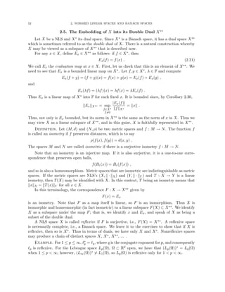
21. 1.2. LEBESGUE MEASURE AND INTEGRATION 21
Proposition 1.39. If f ∈ L(Ω), where Ω is measurable, and if
Z
A
f(x) dx = 0
for every measurable A ⊂ Ω, then f = 0 a.e. on Ω.
Proof. Suppose not. Decompose f as f = f1 + if2 = f+
1 − f−
1 + i(f+
2 − f−
2 ). At least one
of f±
1 , f±
2 is not zero a.e. Let g denote one such component of f. Thus g ≥ 0 and g is not zero
a.e. on Ω. However,
R
A g(x) dx = 0 for every measurable A ⊂ Ω. Let
An = {x ∈ Ω : g(x) 1/n} .
Then µ(An) = 0 ∀ n and A0 =
S∞
n=1 An = {x ∈ Ω : g(x) 0}. But µ(A0) = µ(
S∞
n=1 An) ≤
P∞
n=1 µ(An) = 0, contradicting the fact that g is not zero a.e.
We will not use the following, but it is interesting. It shows that Riemann integration is
restricted to a very narrow class of functions, whereas Lebesgue integration is much more general.
Proposition 1.40. If f is bounded on a compact set [a, b] ⊂ R, then f is Riemann integrable
on [a, b] if and only if f is continuous at a.e. point of [a, b].
The Lebesgue integral is absolutely continuous in the following sense.
Theorem 1.41. If f ∈ L(Ω), then
R
A |f| dx → 0 as µ(A) → 0, where A ⊂ Ω is measurable.
That is, given 0, there is δ 0 such that
Z
A
|f(x)| dx ≤
whenever µ(A) δ.
Proof. Given 0, there is a simple function s(x) such that
Z
A
|f(x) − s(x)| dx ≤ /2 ,
by the definitionn of the Lebesgue integral. Moreover, by the proof of the existance of s(x), we
know that we can take s(x) bounded:
|s(x)| ≤ M()
for some M(). Then on A ⊂ Ω measurable,
Z
A
|s(x)| dx ≤ µ(A)M(),
so if µ(A) δ ≡ /2M(), then
Z
A
|f(x)| dx ≤
Z
A
|f(x) − s(x)| dx +
Z
A
|s(x)| dx ≤ /2 + /2 = .
Theorem 1.34 states that we can approximate a measurable f by a sequence of simple
functions. We can go further, and approximate by a sequence of continuous functions, at least
when we control things near infinity. Let C0(Ω) be the set of continuous functions with compact
support, i.e., continuous functions that vanish outside a bounded set.

22. 22 1. PRELIMINARIES
Theorem 1.42 (Lusin’s Theorem). Suppose that f is measurable on Ω is such that f(x) = 0
for x 6∈ A, where A has finite measure. Given 0, there is g ∈ C0(Ω) such that the measure
of the set where f and g differ is less than . Moreover,
sup
x∈Ω
|g(x)| ≤ sup
x∈Ω
|f(x)| .
A proof can be found in, e.g., [Ru2]. The following lemma is easily demonstrated (and left
to the reader), but it turns out to be quite useful.
Lemma 1.43 (Chebyshev’s Inequality). If f ≥ 0 and Ω ⊂ Rd are measurable, then
µ({x ∈ Ω : f(x) α}) ≤
1
α
Z
Ω
f(x) dx
for any α 0.
We conclude our overview of Lebesgue measure and integration with the three basic con-
vergence theorems, Fubini’s Theorem on integration over product spaces, and the Fundamental
Theorem of Calculus, each without proof. For the first three results, assume that Ω ⊂ Rd is
measurable.
Theorem 1.44 (Lebesgue’s Monotone Convergence Theorem). If {fn}∞
n=1 is a sequence of
measurable functions satisfying 0 ≤ f1(x) ≤ f2(x) ≤ · · · for a.e. x ∈ Ω, then
lim
n→∞
Z
Ω
fn(x) dx =
Z
Ω
lim
n→∞
fn(x)
dx .
Theorem 1.45 (Fatou’s Lemma). If {fn}∞
n=1 is a sequence of nonnegative, measurable func-
tions, then
Z
Ω
lim inf
x→∞
fn(x)
dx ≤ lim inf
n→∞
Z
Ω
fn(x) dx .
Theorem 1.46 (Lebesgue’s Dominated Convergence Theorem). Let {fn}∞
n=1 be a sequence
of measurable functions that converge pointwise for a.e. x ∈ Ω. If there is a function g ∈ L(Ω)
such that
|fn(x)| ≤ g(x) for every n and a.e. x ∈ Ω,
then
lim
n→∞
Z
Ω
fn(x) dx =
Z
Ω
lim
n→∞
fn(x)
dx .
Theorem 1.47 (Fubini’s Theorem). Let f be measurable on Rn+m. If at least one of the
integrals
I1 =
Z
Rn+m
f(x, y) dx dy ,
I2 =
Z
Rm
Z
Rn
f(x, y) dx
dy ,
I3 =
Z
Rn
Z
Rm
f(x, y) dy
dx
exists in the Lebesgue sense (i.e., when f is replaced by |f|) and is finite, then each exists and
I1 = I2 = I3.

23. 1.3. EXERCISES 23
Note that in Fubini’s Theorem, the claim is that the following are equivalent:
(i) f ∈ L(Rn+m),
(ii) f(·, y) ∈ L(Rn) for a.e. y ∈ Rm and
R
Rn f(x, ·) dx ∈ L(Rm),
(iii) f(x, ·) ∈ L(Rm) for a.e. x ∈ Rn and
R
Rm f(·, y) dy ∈ L(Rn),
and the three full integrals agree. Among other things, f being measurable on Rn+m implies
that f(·, y) is measurable for a.e. y ∈ Rm and f(x, ·) is measurable for a.e. x ∈ Rn. Note also
that we cannot possibly claim anything about every x ∈ Rn and/or y ∈ Rm, but only about
almost every point.
Theorem 1.48 (Fundamental Theorem of Calculus). If f ∈ L([a, b]) and
F(x) =
Z x
a
f(t) dt ,
then F0(x) = f(x) for a.e. x ∈ [a, b]. Conversely, if F is differentiable everywhere (not a.e.!) on
[a, b] and F0 ∈ L([a, b]), then
F(x) − F(a) =
Z x
a
F0
(t) dt
for any x ∈ [a, b].
1.3. Exercises
1. Show that the following define a topology T on X, where X is any nonempty set.
(a) T = {∅, X}. This is called the trivial topology on X.
(b) TB = {{x} : x ∈ X} is a base. This is called the discrete topology on X.
(c) Let T consist of ∅ and all subsets of X with finite complements. If X is finite, what
topology is this?
2. Let X = {a, b} and T = {∅, {a}, X}. Show directly that there is no metric d : X × X → R
that is compatible with the topology. Thus not every topological space is metrizable.
3. Prove that if A ⊂ X, then ∂A is closed and
Ā = A◦
∪ ∂A , A◦
∩ ∂A = ∅ .
Moreover,
∂A = ∂Ac
= {x ∈ X : every open E containing x intersects both A and Ac
} .
4. Prove that if (X, T ) is Hausdorff, then every set consisting of a single point is closed. More-
over, limits of sequences are unique.
5. Prove that a set A ⊂ X is open if and only if, given x ∈ A, there is an open E such that
x ∈ E ⊂ A.
6. Prove that a mapping of X into Y is continuous if and only if the inverse image of every
closed set is closed.
7. Prove that if f is continuous and lim
n→∞
xn = x, then lim
n→∞
f(xn) = f(x).
8. Suppose that f(x) = y. Let Bx be a base at x ∈ X, and C a base at y ∈ Y . Prove that f is
continuous at x if and only if for each C ∈ Cy there is a B ∈ Bx such that B ⊂ f−1(C).
9. Show that every metric space is Hausdorff.

24. 24 1. PRELIMINARIES
10. Suppose that F : X → R. Characterize all topologies T on X that make f continuous.
Which is the weakest? Which is the strongest?
11. Construct an infinite open cover of (0, 1] that has no finite subcover. Find a sequence in
(0, 1] that does not have a convergent subsequence.
12. Prove that the continuous image of a compact set is compact.
13. Prove that a one-to-one continuous map of a compact space X onto a Hausdorff space Y is
necessarily a homeomorphism.
14. Prove that if f : X → R is continuous and X compact, then f takes on its maximum and
minimum values.
15. Show that the Borel sets B is the collection of all sets that can be constructed by a countable
number of basic set operations, starting from open sets. The basic set operations consist of
taking unions, intersections, or complements.
16. Prove each of the following.
(a) If f : Rd → R is measurable and g : R → R is continuous, then g ◦ f is measurable.
(b) If Ω ⊂ Rd is measurable and f : Ω → R is continuous, than f is measurable.
17. Let x ∈ Rd be fixed. Define dx for any A ⊂ Rd by
dx(A) =
(
1 if x ∈ A ,
0 if x 6∈ A .
Show that dx is a measure on the Borel sets B. This measure is called the Dirac or point
measure at x.
18. The Divergence Theorem from advanced calculus says that if Ω ⊂ Rd has a smooth boundary
and v ∈ (C1(Ω̄))d is a vector-valued function, then
Z
Ω
∇ · v(x) dx =
Z
∂Ω
v(x) · ν(x) ds(x) ,
where ν(x) is the outward pointing unit normal vector to Ω for any x ∈ ∂Ω, and ds(x) is
the surface differential (i.e., measure) on ∂Ω. Note that here dx is a d-dimensional measure,
and ds is a (d − 1)-dimensional measure.
(a) Interpret the formula when d = 1 in terms of the Dirac measure.
(b) Show that for φ ∈ C1(Ω̄),
∇ · (φv) = ∇φ · v + φ∇ · v .
(c) Let φ ∈ C1(Ω̄) and apply the Divergence Theorem to the vector φv in place of v. We
call this new formula integration by parts. Show that it reduces to ordinary integration by
parts when d = 1.
19. Prove that if f ∈ L(Ω) and g : Ω → R, where g and Ω are measurable and g is bounded,
then fg ∈ L(Ω).
20. Construct an example of a sequence of nonnegative measurable functions from R to R that
shows that strict inequality can result in Fatou’s Lemma.

25. 1.3. EXERCISES 25
21. Let
fn(x) =



1
n
, |x| ≤ n ,
0 , |x| n .
Show that fn(x) → 0 uniformly on R, but
Z ∞
−∞
fn(x) dx = 2 .
Comment on the applicability of the Dominated Convergence Theorem.
22. Let
f(x, y) =





1 , 0 ≤ x − y ≤ 1 ,
−1 , 0 ≤ y − x ≤ 1 ,
0 , otherwise.
Show that Z ∞
0
Z ∞
0
f(x, y) dx
dy 6=
Z ∞
0
Z ∞
0
f(x, y) dy
dx .
Comment on the applicability of Fubini’s Theorem.
23. Suppose that f is integrable on [a, b], and define
F(x) =
Z x
a
f(t) dt .
Prove that F is continuous on [a, b]. (In fact, F0 = f a.e., but it is more involved to prove
this.)

27. CHAPTER 2
Normed Linear Spaces and Banach Spaces
Functional Analysis grew out of the late 19th century study of differential and integral
equations arising in physics, but it emerged as a subject in its own right in the first part of
the 20th century. Thus functional analysis is a genuinely 20th century subject, often the first
one a student meets in analysis. For the first sixty or seventy years of this century, functional
analysis was a major topic within mathematics, attracting a large following among both pure
and applied mathematicians. Lately, the pure end of the subject has become the purview of a
more restricted coterie who are concerned with very difficult and often quite subtle issues. On
the other hand, the applications of the basic theory and even of some of its finer elucidations
has grown steadily, to the point where one can no longer intelligently read papers in much
of numerical analysis, partial differential equations and parts of stochastic analysis without a
working knowledge of functional analysis. Indeed, the basic structures of the theory arises in
many other parts of mathematics and its applications.
Our aim in the first section of this course is to expound the elements of the subject with an
eye especially for aspects that lend themselves to applications.
We begin with a formal development as this is the most efficient path.
2.1. Basic Concepts and Definitions.
Vector spaces are fundamental in science and engineering. They encapsulate notions of
scaling (scalar multiplication) and translation (vector addition). Vector spaces become very
powerful tools when we add the notion of vector size or norm.
Definition. Let X be a vector space over the real numbers R or the complex numbers C.
We say X is a normed linear space (NLS for short) if there is a mapping
k · k : X → R+
= [0, ∞) ,
called the norm on X, satisfying the following set of rules which apply to x, y ∈ X and λ ∈ R
or C:
(a) kλxk = |λ| kxk ,
(b) kxk = 0 if and only if x = 0 ,
(c) kx + yk ≤ kxk + kyk (triangle inequality).
In situations where more than one NLS is under consideration, it is often convenient to write
k · kX for the norm on the space X to indicate which norm is connoted.
A NLS X is finite dimensional if it is finite dimensional as a vector space, which is to
say there is a finite collection {xn}N
n=1 ⊂ X such that any x ∈ X can be written as a linear
combination of the {xn}N
n=1, viz.
x = λ1x1 + λ2x2 + · · · + λN xN ,
where the λi are scalars (member of the ground field R or C). Otherwise, X is called infinite
dimensional. Interest here is mainly in infinite-dimensional spaces.
27

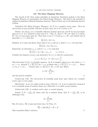
28. 28 2. NORMED LINEAR SPACES AND BANACH SPACES
Remark. In a good deal of the theory developed here, it will not matter for the outcome
whether the NLS’s are real or complex vector spaces. When this point is moot, we will often
write F rather than R or C. The reader should understand when the symbol F appears that it
stands for either R or for C, and the discussion at that juncture holds for both.
Examples. (a) Consider Fd with the usual Euclidean length of a vector x = (x1, ..., xd)
denoted |x| =
Pd
n=1 |xn|2
1/2
. If we define, for x ∈ Fd, kxk = |x|, then (Fd, k · k) is a finite
dimensional NLS.
(b) Let a and b be real numbers, a b, with a = −∞ or b = +∞ allowed as possible values.
Then
C([a, b]) =
f : [a, b] → F : f is continuous and sup
x∈[a,b]
|f(x)| ∞
.
We impose a vector space structure by pointwise multiplication and addition; that is, for x ∈ [a, b]
and λ ∈ F, we define
(f + g)(x) = f(x) + g(x) and (λf)(x) = λf(x) .
For f ∈ C([a, b]), let
kfkC([a,b]) = sup
x∈[a,b]
|f(x)| ,
which is easily shown to be a norm. Thus, C([a, b]), k · kC([a,b])
is a NLS, which is also infinite
dimensional. (To see this latter fact, the reader can consider the impossibility of finding a finite
basis for the periodic base functions of Fourier series on a bounded interval.)
(c) We can impose a different norm on the space C([a, b]) defined by
kfkL1([a,b]) =
Z b
a
|f(x)| dx .
Again, it is easy to verify that C([a, b]), k·kL1([a,b])
is a NLS, but it is different from C([a, b]), k·
kC([a,b])
. These two NLS’s have the same set objects and the same vector space structure, but
different norms, i.e., they measure sizes differently.
Further examples arise as subspaces of NLS’s. This fact follows directly from the definitions,
and is stated formally below.
Proposition 2.1. If (X, k · k) is a NLS and V ⊂ X is a linear subspace, then (V, k · k) is a
NLS.
Let (X, k · k) be a NLS. Then X is a metric space if we define a metric d on X by
d(x, y) = kx − yk .
To see this, just note the following: for x, y, z ∈ X,
d(x, x) = kx − xk = k0k = 0 ,
0 = d(x, y) = kx − yk =⇒ x − y = 0 =⇒ x = y ,
d(x, y) = kx − yk = k − (y − x)k = | − 1| ky − xk = d(y, x) ,
d(x, y) = kx − yk = kx − z + z − yk
≤ kx − zk + kz − yk = d(x, z) + d(z, y) .
Consequently, the concepts of elementary topology are available in any NLS. In particular, we
may talk about open sets and closed sets in a NLS.

29. 2.1. BASIC CONCEPTS AND DEFINITIONS. 29
A set U ⊂ X is open if for each x ∈ U, there is an r 0 (depending on x in general) such
that
Br(x) = {y ∈ X : d(y, x) r} ⊂ U .
The set Br(x) is referred to as the (open) ball of radius r about x. A set F ⊂ X is closed if
Fc = X r F = {y ∈ X, y /
∈ F} is open. As with any metric space, F is closed if and only if
it is sequentially closed. That is, F is closed means that whenever {xn}∞
1 ⊂ F and xn → x as
n → ∞ for the metric, then it must be the case that x ∈ F.
Proposition 2.2. In a NLS X, the operations of addition, + : X × X → X and scalar
multiplication, · : F × X → X, and the norm, k · k : X → R, are continuous.
Proof. Let {xn}∞
n=1 and {yn}∞
n=1 be sequences in X converging to x, y ∈ X, respectively.
Then
k(xn + yn) − (x + y)k = k(xn − x) + (yn − y)k ≤ kxn − xk + kyn − yk → 0 .
We leave scalar multiplication for the reader, which requires the fact that a convergent sequence
of scalars is bounded.
For the norm,
kxk ≤ kx − xnk + kxnk ≤ 2kx − xnk + kxk ,
so we conclude that limn→∞ kxnk = kxk, i.e., the norm is continuous.
Recall that a sequence {xn}∞
n=1 in a metric space (X, d) is called a Cauchy sequence if
lim
n,m→∞
d(xn, xm) = 0 ;
or equivalently, given ε 0, there is an N = N(ε) such that if n, m ≥ N, then
d(xn, xm) ≤ ε .
A metric space is called complete if every Cauchy sequence converges to a point in X. A
NLS (X, k · k) that is complete as a metric space is called a Banach space after the Polish
mathematician Stefan Banach, who was a pioneer in the subject.
Examples. (a) The spaces Rd and Cd are complete as we learn in advanced calculus or
elementary analysis.
(b) For a and b in [−∞, ∞], a b, the space C([a, b]), k · kC([a,b])
is complete, since the
uniform limit of continuous functions is continuous. That is, a Cauchy sequence will converge
to a continuous function.
(c) The space C([a, b]), k · kL1([a,b])
is not complete. To see this, suppose that a = −1 and
b = 1 (we can translate and scale if this is not true) and define for n = 1, 2, 3, ...,
fn(x) =





1 if x ≤ 0 ,
1 − nx if 0 x 1/n ,
0 if x ≥ 1/n .
Each fn ∈ C([−1, 1]), and this is a Cauchy sequence for the given norm, since
Z 1
−1
|fn(x) − fm(x)| dx ≤
Z 1
0
(|fn(x)| + |fm(x)|) dx ≤
1
2n
+
1
2m

30. 30 2. NORMED LINEAR SPACES AND BANACH SPACES
can be made as small as we like for n and m large enough (note that the sequence is not Cauchy
using the norm k·kC([−1,1])!). However, fn does not converge in C([−1, 1]), since it must converge
to 1 for x 0 and to 0 for x 0, which is not a continuous function.
By convention, unless otherwise specified, we use the norm k · k = k · kC([a,b]) on C([a, b]),
which makes it a Banach space.
If X is a linear space over F and d is a metric on X induced from a norm on X, then for all
x, y, a ∈ X and λ ∈ F,
d(x + a, y + a) = d(x, y) and d(λx, λy) = |λ|d(x, y) . (2.1)
Suppose now that X is a linear space over F and d is a metric on X satisfying (2.1). Is it
necessarily the case that there is a norm k · k on X such that d(x, y) = kx − yk? We leave this
question for the reader to ponder.
If X is a vector space and k·k1 and k · k2 are two norms on X, they are said to be equivalent
norms if there exist constants c, d 0 such that
ckxk1 ≤ kxk2 ≤ dkxk1 (2.2)
for all x ∈ X. Equivalent norms do not measure size in the same way, but, up to the constants
c and d, they agree when something is “small” or “large.”
It is a fundamental fact, as we will see later, that on a finite-dimensional NLS, any pair of
norms is equivalent, whereas this is not the case in infinite dimensional spaces. For example, if
f ∈ C([0, 1]), then
kfkL1([0,1]) ≤ kfkC([0,1]) ,
but the opposite bound is lacking. To see this, consider the sequence
fn(x) =





n2x if x ≤ 1/n ,
2n − n2x if 1/n x 2/n ,
0 if x ≥ 2/n ,
for which
kfnkC([0,1]) = n but kfkL1([0,1]) = 1 .
If k · k1 and k · k2 are two equivalent norms on a NLS X as in (2.2), then the collections O1
and O2 of open sets induced by these two norms as just outlined are the same. To see this, let
Bi
r(x) be the ball about x ∈ X of radius r measured using norm k · ki. Then
B1
r/c(x) ⊂ B2
r (x) ⊂ B1
r/d(x)
shows that our open balls are nested. Thus topologically, (X, k · k1) and (X, k · k2) are indis-
tinguishable. Moreover, finite dimensional NLS’s have a unique topological structure, whereas
infinite dimensional NLS’s may have many distinct topologies.
Convexity is an important property in vector spaces.
Definition. A set C in a linear space X over F is convex if whenever x, y ∈ C, then
tx + (1 − t)y ∈ C
whenever 0 ≤ t ≤ 1.
Proposition 2.3. Suppose (X, k · k) is a NLS and r 0. For any x ∈ X, Br(x) is convex.

31. 2.1. BASIC CONCEPTS AND DEFINITIONS. 31
Proof. Let y, z ∈ Br(x) and t ∈ [0, 1] and compute as follows:
kty + (1 − t)z − xk = kt(y − x) + (1 − t)(z − x)k
≤ kt(y − x)k + k(1 − t)(z − x)k
= |t| ky − xk + |1 − t| kz − xk
tr + (1 − t)r = r .
Thus, Br(x) is convex.
One reason vector spaces are so important and ubiquitous is that they are the natural
domain of definition for linear maps, and the latter pervade mathematics and its applications.
Remember, a linear map is one that commutes with addition and scalar multiplication, so that
T(x + y) = T(x) + T(y) ,
T(λx) = λT(x) ,
for x, y ∈ X, λ ∈ F. For linear maps, we often write Tx for T(x), leaving out the parentheses.
The scaling property requires that T(0) = 0 for every linear map.
A set M ⊂ X of a NLS X is said to be bounded if there is R 0 such that M ⊂ BR(0);
that is,
kxk ≤ R ∞ for all x ∈ M .
An operator T : X → Y , X and Y NLS’s, is bounded if it takes bounded sets to bounded sets.
(Note that this does not require that the entire image of T be bounded!)
Proposition 2.4. If X and Y are NLS’s and T : X → Y is linear, then T is bounded if
and only if there is C 0 such that
kTxkY ≤ CkxkX for all x ∈ X .
Proof. The result follows from scaling considerations. Suppose first that T is bounded.
For M = B1(0), there is R 0 such that
kTykY ≤ R for all y ∈ M .
Now let x ∈ X be given. If x = 0, the conclusion holds trivially. Otherwise, let y = x/2kxkX ∈
M. Then
kTxkY = T(2kxkXy) Y
= 2kxkXTy Y
= 2kxkXkTykY ≤ 2RkxkX ,
which is the conclusion with C = 2R.
Conversely, suppose that there is C 0 such that
kTxkY ≤ CkxkX for all x ∈ X .
Let M ⊂ BR(0) be bounded and fix x ∈ M. Then
kTxkY ≤ CkxkX ≤ CR ∞,
so T takes a bounded set to a bounded set.
On the one hand, the linear maps are the natural (i.e., structure preserving) maps on a
vector space. On the other hand, the natural mappings between topological spaces, and metric
spaces in particular, are the continuous maps. If (X, d) and (Y, ρ) are two metric spaces and

32. 32 2. NORMED LINEAR SPACES AND BANACH SPACES
f : X → Y is a function, then f is continuous if for any x ∈ X and ε 0, there exists a
δ = δ(x, ε) 0 such that
d(x, y) ≤ δ implies ρ(f(x), f(y)) ≤ ε .
This is to say, for NLS’s,
kx − yk ≤ δ implies kf(x) − f(y)k ≤ ε .
If (X, k·kX) and (Y, k·kY ) are NLS’s, then they are simultaneously linear spaces and metric
spaces. Thus one might expect the collection
B(X, Y ) = {T : X → Y : T is linear and continuous} (2.3)
to be an interesting class of mappings that are consistent with both the algebraic and metric
structures of the underlying spaces. Continuous linear mappings between NLS’s are often called
bounded operators or bounded linear operators or continuous linear operators.
Example. If X = Rd1 and Y = Rd2 , then B(Rd1 , Rd2 ) is precisely the set of (real) d1 × d2
matrices, which are easily seen to be continuous linear operators. In fact, in finite dimensions,
every linear map is continuous. This is not the case in infinite dimensions.
Proposition 2.5. Let X and Y be NLS’s and T : X → Y a linear map. The following are
equivalent:
(a) T is continuous,
(b) T is continuous at some point,
(c) T is bounded.
Proof. (a =⇒ b) Trivial.
(b =⇒ c) Suppose T is continuous at x0 ∈ X. Then there is a δ = δ(1, x0) 0 such that
kx − x0kX ≤ δ implies kTx − Tx0kY ≤ 1 . (2.4)
But by linearity Tx − Tx0 = T(x − x0). Thus, (2.4) is equivalent to the condition
kykX ≤ δ implies kTykY ≤ 1 .
Hence, it follows readily that if x ∈ X, x 6= 0, then
kTxkY =
kxkX
δ
T
δ
kxkX
x
Y
=
1
δ
T
δ
kxkX
x
Y
kxkX ≤
1
δ
kxkX ,
since
δ
kxkX
x
X
= δ .
(c =⇒ a) It is supposed that T is linear and bounded, so there is a C 0 such that
kTxkY ≤ CkxkX for all x ∈ X .
Let ε 0 be given and let δ = ε/C. Suppose kx − x0kX ≤ δ. Then
kTx − Tx0kY = kT(x − x0)kY ≤ Ckx − x0kX ≤ ε .
Therefore T is continuous at x0, and x0 was an arbitrary point in X.

33. 2.1. BASIC CONCEPTS AND DEFINITIONS. 33
Let X, Y be NLS’s and let T ∈ B(X, Y ) be a continuous linear operator from X to Y . We
know that T is therefore bounded on any bounded set of X, so the quantity
kTk = kTkB(X,Y ) = sup
x∈B1(0)
kTxkY (2.5)
is finite. The notation makes it clear that this mapping k · kB(X,Y ) : B(X, Y ) → [0, ∞) is
expected to be a norm. There are several things to check.
We begin by noting that B(X, Y ) is a vector space in its own right if we define S + T and
λT by
(S + T)(x) = Sx + Tx and (λS)(x) = λSx
for all x ∈ X and λ ∈ F.
Proposition 2.6. Let X and Y be NLS’s. The formula (2.5) defines a norm on B(X, Y ).
Moreover, if T ∈ B(X, Y ), then
kTk = sup
kxkX =1
kTxkY = sup
x6=0
kTxkY
kxkX
. (2.6)
If Y is a Banach space, then so is B(X, Y ) with this norm.
Proof. We first show that k·kB(X,Y ) is a norm. If T is the zero map, then clearly kTk = 0.
On the other hand, if kTk = 0, then T vanishes on the unit ball. For any x ∈ X, x 6= 0, write
x = 2kxk(x/2kxk) = 2kxky. Then y is in the unit ball, so T(y) = 0. Then T(x) = 2kxkT(y) = 0;
thus T ≡ 0. Plainly, by definition of scalar multiplication
kλTk = sup
B1(0)
k(λT)(x)kY = |λ| sup
B1(0)
kTxkY = |λ| kTk .
The triangle inequality is just as simple:
kT + Sk = sup
x∈B1(0)
k(T + S)(x)kY = sup
x∈B1(0)
kTx + SxkY
≤ sup
x∈B1(0)
n
kTxkY + kSxkY
o
≤ sup
x∈B1(0)
kTxkY + sup
x∈B1(0)
kSxkY = kTk + kSk .
Thus (B(X, Y ), k · kB(X,Y )) is indeed a NLS.
The alternative formulas for the norm expressed in (2.6) are straightforward to deduce.
Notice that the last formula makes it obvious that for all x ∈ X and T ∈ B(X, Y ),
kTxkY ≤ kTkB(X,Y )kxkX , (2.7)
an inequality that will find frequent use.
The more interesting fact is that B(X, Y ) is complete if we only assume Y is complete.
This simple result has far-reaching consequences. To establish this point, suppose {Tn}∞
n=1 is a
Cauchy sequence in B(X, Y ). We must show it converges in B(X, Y ). Let x ∈ X and consider
the sequence {Tnx}∞
n=1 in Y . Because of (2.7), it follows that
kTnx − TmxkY ≤ kTn − TmkB(X,Y )kxkX,
and thus {Tnx}∞
n=1 is seen to be Cauchy in Y . As Y is a Banach space, {Tnx}∞
n=1 must converge
to some element of Y that depends upon x of course; call this element Tx. There is thus
established a correspondence
x 7−→ Tx

34. 34 2. NORMED LINEAR SPACES AND BANACH SPACES
between X and Y . We claim it is a continuous linear correspondence, whence T ∈ B(X, Y ). It
is further asserted that Tn → T in B(X, Y ).
First note that
T(x + y) = lim
n→∞
Tn(x + y) = lim
n→∞
{Tnx + Tny}
= lim
n→∞
Tnx + lim
n→∞
Tny = Tx + Ty .
Similarly, T(λx) = λTx for x ∈ X and λ ∈ F. Thus T is a linear map. To see that T is a
bounded map, first note that {Tn}∞
n=1, being Cauchy, must be a bounded sequence. For there
is an N such that if n ≥ N, then
kTn − TN k ≤ 1 ,
say. By the triangle inequality, this means
kTnk ≤ kTN k + 1 ,
for n ≥ N. The initial segment, {T1, T2, . . . , TN−1} of the sequence is bounded since it is finite,
say kTjk ≤ K for 1 ≤ j ≤ N − 1. It therefore transpires that
kTkk ≤ max{K, kTN k + 1} = M ,
say, for all k. From this it follows at once that T is a bounded operator; for if x ∈ X, then
kTxkY = lim
n→∞
kTnxkY ≤ lim sup
n→∞
kTnkB(X,Y )kxkX ≤ Mkxk .
Finally, we check that Tn → T in B(X, Y ). Let x ∈ B1(0) in X and observe that
kTx − TnxkY = lim
m→∞
kTmx − TnxkY = lim
m→∞
k(Tm − Tn)xk
≤ lim sup
m→∞
kTm − TnkB(X,Y )kxkX ≤ ε(n) .
Since x was an arbitrary element in B1(0), this means
kT − TnkB(X,Y ) ≤ ε(n)
and because {Tk}∞
k=1 is Cauchy, ε(n) → 0 as n → ∞.
The structure of bounded linear maps T : X → Y on infinite dimensional spaces can be
quite complex. However, it will turn out to be quite a fruitful to study the simpler case, albeit
still quite complex, of a map T : X → F, for which the range has a single dimension.
Definition. Let X be a NLS over F. The dual space X∗ of X is the Banach space B(X, F).
The elements of X∗ are called bounded linear functionals on X.
The dual space is complete because R and C are complete.
2.2. Some Important Examples
2.2.1. Finite dimensional spaces. Let X be a vector space of dimension d ∞ over F,
and let {en}d
n=1 ⊂ X be a basis, which is to say that for any x ∈ X, there are unique xn ∈ F
such that
x =
d
X
n=1
xn en .
We define a map T : X → Fd by T(x) = (x1, ..., xd), which gives a one-to-one correspondance
between X and Fd. This map, called the coordinate mapping, is easily seen to be linear, so we

35. 2.2. SOME IMPORTANT EXAMPLES 35
have a vector space isomorphism between the spaces. Consequently, X and Fd have the same
vector space structure. That is, given a dimension d, there is only one vector space structure of
the given dimension (for the field F).
Define for 1 ≤ p ≤ ∞ the map k · k`p : Fd → [0, ∞) by
kxk`p =





d
X
n=1
|xn|p
1/p
for p ∞ ,
maxn=1,...,d |xn| for p = ∞ .
It is easy to verify that kxk`1 and kxk`∞ are norms on Fd. In fact, the zero and scaling properties
of a norm are easily verified for k · k`p , but we need a few facts before we can verify the triangle
inequality. Once done, note that then also kT(·)k`p is a norm on X.
The following simple inequality turns out to be quite useful in practice.
Lemma 2.7. Let 1 p ∞ and let q denote the conjugate exponent to p defined by
1
p
+
1
q
= 1 .
If a and b are nonnegative real numbers, then
ab ≤
ap
p
+
bq
q
, (2.8)
with equality if and only if ap/bq = 1. Moreover, for any 0, then there is C = C(p, ) 0
such that
ab ≤ ap
+ Cbq
.
Proof. The function u : [0, ∞) → R given by
u(t) =
tp
p
+
1
q
− t
has minimum value 0, attained only with t = 1. Apply this fact to t = ab−q/p to obtain main
result. Replace ab by [(p)1/pa][(p)−1/pb] to obtain the final result.
This leads us immediately to Hölder’s Inequality. When p = 2, the inequality is also called
the Cauchy-Schwarz Inequality.
Theorem 2.8 (Hölder’s Inequality). Let 1 ≤ p ≤ ∞ and let q denote the conjugate exponent
(i.e., 1/p + 1/q = 1, with the convention that q = ∞ if p = 1 and q = 1 if p = ∞). If x, y ∈ Fd,
then
d
X
n=1
|xnyn| ≤ kxk`p kyk`q .
Proof. The result is trivial if either p or q is infinity. Otherwise, simply apply (2.8) to
a = |xn|/kxk`p and b = |yn|/kyk`q and sum on n to see that
d
X
n=1
|xn|
kxk`p
|yn|
kyk`q
≤
d
X
n=1
|xn|p
pkxkp
`p
+
d
X
n=1
|yn|q
qkykq
`q
=
1
p
+
1
q
= 1 .
Thus the conclusion follows.

36. 36 2. NORMED LINEAR SPACES AND BANACH SPACES
We can now finish our proof that each k·k`p is in fact a norm on Fd; it remains only to show
the triangle inequality for 1 p ∞. For x, y ∈ Fd, simply apply Hölder’s inequality twice as
follows:
kx + ykp
`p
=
d
X
n=1
|xn + yn|p
≤
d
X
n=1
|xn + yn|p−1
(|xn| + |yn|)
≤
d
X
n=1
|xn + yn|(p−1)q
1/q
kxk`p + kyk`p
.
Since (p − 1)q = p and 1 − 1/q = 1/p, we have the triangle inequality
kx + yk`p ≤ kxk`p + kyk`p
as desired.
Proposition 2.9. Let 1 ≤ p ≤ ∞. For any x ∈ Fd,
kxk`∞ ≤ kxk`p ≤ d1/p
kxk`∞ ,
with equality possible.
This result is trivial, and shows that all the `p-norms kxk`p , 1 ≤ p ≤ ∞, are equivalent on
Fd, and it gives the optimal bounding constants with respect to the `∞-norm.
A fundamental difference between finite and infinite dimensional spaces NLS’s is that in
finite dimensions, a closed and bounded set is always compact, but this statement turns out to
be untrue in infinite dimensions. This is closely related to another fundamental difference: in
finite dimensions, all norms are equivalent, and so there is in fact only one norm topology.
Proposition 2.10. Let X be a finite dimensional NLS. All norms on X are equivalent.
Moreover, a subset of X is compact if and only if it is closed and bounded.
Proof. Let d be the dimension of X, and let {en}d
n=1 be a basis. We defined earlier the
coordinate mapping T : X → Fd. Let k · k denote any norm of X, and let
kxk1 = kT(x)k`1
be a second norm. We will show that these two norms are equivalent, which then implies that
any pair are equivalent.
The space (X, k · k1) is essentially Fd, on which we assume the norm k · k`1 . In fact, by
definition of the norm k·k1, the coordinate map T : (X, k·k1) → Fd is bounded, i.e., continuous,
as is its inverse, which is also a linear function. Thus, (X, k · k1) and Fd are homeomorphic as
topological spaces, and also isomorphic as vector spaces. The Heine-Borel Theorem states that
every closed and bounded subset of Fd is compact, so the same is true of (X, k·k1). In particular,
S1
1 = {x ∈ X : kxk1 = 1} is compact.
For x ∈ X,
kxk =
d
X
n=1
xnen ≤
d
X
n=1
|xn| kenk ≤ Ckxk1 ,
where C = maxn kenk ∞. This is one of the two bounds needed to show that the norms are
equivalent. Moreover, we conclude that the topology on X generated by k · k1 is stronger than
that generated by k · k (i.e., every open set of (X, k · k) is an open set of (X, k · k1)). Because a
norm is continuous in its own topology, we conclude that the function k · k : (X, k · k1) → R is

37. 2.2. SOME IMPORTANT EXAMPLES 37
also continuous (i.e., the inverse image of every open set in R is open in (X, k · k), and thus also
open in (X, k · k1)).
Now let
a = inf
x∈S1
1
kxk .
Since S1
1 is compact and k · k is continuous, the function must take on its minimal value. That
is, there is some x1 ∈ S1
1 such that a = kx1k, which is then strictly positive since x1 6= 0. That
is, for any x ∈ X, scaling implies that
kxk ≥ akxk1 , a 0 ,
which is the other bound needed and shows that in fact the two norms are equivalent. Finally,
the compactness result now holds in general, since there is only one norm topology on X.
Within the course of the above proof, we established that for a given dimension d, there is
only one NLS structure. Infinite dimensional spaces are more interesting.
Corollary 2.11. Every NLS of dimension d ∞ is isomorphic and homeomorphic to Fd,
and so is a Banach space.
We leave the following corollary for the reader.
Corollary 2.12. If X and Y are NLS’s, X finite dimensional, and T : X → Y linear,
then T is bounded. Moreover, the dual space X∗ is isomorphic and homeomorphic to Fd.
2.2.2. The spaces `p. Let p lie in the range [1, ∞) and define the real vector spaces and
norms
`p =
x = {xn}∞
n=1 : xn ∈ F and kxk`p =
∞
X
n=1
|xn|p
1/p
∞
,
and, if p = ∞,
`∞ =
n
x = {xn}∞
n=1 : xn ∈ F and kxk`∞ = sup
n
|xn| ∞
o
.
These spaces are NLS’s over F, since it is easy to verify that they are vector spaces and since
k · k`p can be shown to be a norm using the techniques of the previous section. In fact, we have
the infinite dimensional version of Hölder’s Inequality.
Theorem 2.13 (Hölder’s Inequality in `p). Let 1 ≤ p ≤ ∞ and let q denote the conjugate
exponent (i.e., 1/p + 1/q = 1). If x ∈ `p and y ∈ `q, then
∞
X
n=1
|xnyn| ≤ kxk`p kyk`q .
We leave the details of the proof of these assertions to the reader. Moreover, it is not difficult
to show that
`p ⊂ `q whenever p ≤ q .
Moreover, if 1 ≤ p ∞, `p is countably infinite dimensional, having the basis {ei}∞
i=1, where
ei
n = 0 except en
n = 1. In infinite dimensions, by a basis, we mean a set for which the set of
finite linear combinations is dense in the space; that is, our infinite series must converge in the
norm of the space. Thus, {ei}∞
i=1 is not a basis for `∞, since infinite series do not converge in
the `∞-norm.

38. 38 2. NORMED LINEAR SPACES AND BANACH SPACES
Let c0 ⊂ `∞ be the linear subspace defined as
c0 =
n
{xn}∞
n=1 : lim
n→∞
xn = 0
o
,
which is a NLS using norm k · k`∞ . Another interesting subspace is
f =
{xn}∞
n=1 : xn = 0 except for a finite
number of values of n
.
These normed linear spaces are related to each other; indeed if 1 ≤ p ∞,
f ⊂ `p ⊂ c0 ⊂ `∞ .
On f it is easy to construct a linear functional that is not continuous. Consider, for example,
T(x) =
∞
X
n=1
n xn ,
for which ei ∈ f gives T(ei) = i, but keik`∞ = 1. Thus there can be no bound C in the expression
|T(x)| ≤ Ckxk`∞ .
The spaces `p, 1 ≤ p ≤ ∞ are complete, though this requires proof, which follows from the
completeness of F and is left for the exercises. However, if we take the vector space `1 and equip
it with the `∞-norm, this is a NLS, but not a Banach space. To check this, first note that `1 is
a linear subspace of `∞. Indeed, if x = (x1, x2, . . . ) ∈ `1, then
|x|`∞ = sup
i≥1
|xi| ≤
∞
X
j=1
|xj| = |x|`1 ∞ .
Hence `1 with the `∞-norm is a NLS. To see it is not complete, consider the following sequence.
Define {yk}∞
k=1 ⊂ `1 by
yk = (yk,1, yk,2, . . . ) =
1,
1
2
,
1
3
,
1
4
, . . . ,
1
k
, 0, 0, . . .
,
k = 1, 2, 3, . . . . Then {yk}∞
k=1 is Cauchy in the `∞-norm. For if k ≥ m, then
|yk − ym|`∞ ≤
1
m + 1
.
If `1 were complete in the `∞-norm, then {yk}∞
k=1 would converge to some element z ∈ `1. Thus
we would have that
|yk − z|`∞ → 0
as k → ∞. But, for j ≥ 1,
|yk,j − zj| ≤ |yk − z|`∞
where yk,j and zj are the jth-components of yk and z, respectively. In consequence, it is seen
that zj = 1/j for all j ≥ 1. However, the element
z =
1,
1
2
,
1
3
,
1
4
, . . . ,
1
k
,
1
k + 1
, . . .
does not lie in `1, a contradiction. As a corollary, we conclude that an infinite dimensional vector
space may have multiple NLS structures imposed on it.
Lemma 2.14. If p 1, then k · kp is not a norm on `p.

39. 2.2. SOME IMPORTANT EXAMPLES 39
To prove this, show the unit ball B1(0) is not convex, which would otherwise contradict
Prop. 2.3. It is also easy to see directly that the triangle inequality does not always hold. We
leave the details to the reader.
The Hölder inequality implies the existence of continuous linear functionals. Let 1 ≤ p ≤ ∞
and q be conjugate to p. Then any y ∈ `q can be viewed as a function Y : `p → F by
Y (x) =
∞
X
n=1
xn yn for all x ∈ `p . (2.9)
This is clearly a linear functional, and it is bounded, since
|Y (x)| ≤ (kyk`q )kxk`p .
In fact, we leave it to the reader to show that
kY k = kyk`q .
The converse is also true for 1 ≤ p ∞: for any continuous linear functional Y on `p, there
is y ∈ `q such that (2.9) holds. That is, we can identify the dual of `p as `q under the action
defined by (2.9). Again, we leave the details to the exercises, but it should be clear that we need
to define yn = Y (en), where en is from the standard basis. The main concern is justifying that
y ∈ `p. We also have that c∗
0 = `1, but the dual of `∞ is larger that `1.
2.2.3. The Lebesgue spaces Lp(Ω). Let Ω ⊂ Rd be measurable and let 0 p ∞. We
denote by Lp(Ω) the class of all measurable functions f : Ω → F such that
Z
Ω
|f(x)|p
dx ∞ . (2.10)
An interesting point arises here. Suppose f and g lie in Lp(Ω) and that f(x) = g(x) for a.e.
x ∈ Ω. Then as far as integration is concerned, one really cannot distinguish f from g. For
example, if A ⊂ Ω is measurable, then
Z
A
|f|p
dx =
Z
A
|g|p
dx .
Thus within the class of Lp(Ω), f and g are equivalent. This is formalized by modifying the
definition of the elements of Lp(Ω). We declare two measurable functions that are equal a.e. to
be equivalent, and define the elements of Lp(Ω) to be the equivalence classes
[f] = {g : Ω → F : g = f a.e. on Ω}
such that one (and hence all) representative function satisfies (2.10). However, for convenience,
we continue to speak of and denote elements of Lp(Ω) as “functions” which may be modified on
a set of measure zero without consequence. For example, f = 0 in Lp(Ω) means only that f = 0
a.e. in Ω.
The integral (2.10) arises frequently, so we denote it as
kfkp =
Z
Ω
|f(x)|p
dx
1/p
,
and call it the Lp(Ω)-norm. We will indeed show it to be a norm.
A function f(x) is said to be bounded on Ω by K ∈ R if |f(x)| ≤ K for every x ∈ Ω. We
modify this for measurable functions.

40. 40 2. NORMED LINEAR SPACES AND BANACH SPACES
Definition. A measurable function f : Ω → C is essentially bounded on Ω by K if |f(x)| ≤
K for a.e. x ∈ Ω. The infimum of such K is the essential supremum of |f| on Ω, and denoted
ess supx∈Ω |f(x)|.
For p = ∞, we define kfk∞ = ess supx∈Ω |f(x)|. Then for all 0 p ≤ ∞,
Lp(Ω) = {f : kfkp ∞} .
Proposition 2.15. If 0 p ≤ ∞, then Lp(Ω) is a vector space and kfkp = 0 if and only if
f = 0 a.e. in Ω.
Proof. We first show that Lp(Ω) is closed under addition. For p ∞, f, g ∈ Lp(Ω), and
x ∈ Ω,
|f(x) + g(x)|p
≤
|f(x)| + |g(x)|
p
≤ 2p
|f(x)|p
+ |g(x)|p
.
Integrating, there obtains kf + gkp ≤ 2(kfkp
p + kgkp
p)1/p ∞. The case p = ∞ is clear.
For scalar multiplication, note that for α ∈ F,
kαfkp = |α| kfkp ,
so f ∈ Lp(Ω) implies αf ∈ Lp(Ω). The remark that kfkp = 0 implies f = 0 a.e. is clear.
These spaces are interrelated in a number of ways.
Theorem 2.16 (Hölder’s Inequality in Lp). Let 1 ≤ p ≤ ∞ and let q denote the conjugate
exponent defined by
1
p
+
1
q
= 1 (q = ∞ if p = 1, q = 1 if p = ∞).
If f ∈ Lp(Ω) and g ∈ Lq(Ω), then fg ∈ L1(Ω) and
kfgk1 ≤ kfkpkgkq .
If 1 p ∞, equality occurs if and only if |f(x)|p and |g(x)|q are proportional a.e. in Ω.
Proof. The result is clear if p = 1 or p = ∞. Suppose 1 p ∞. Recall that (2.8) implies
that for a, b 0,
ab ≤
ap
p
+
bq
q
,
with equality if and only if ap/bq = 1. If kfkp = 0 or kgkq = 0, then fg = 0 a.e. on Ω and the
result follows. Otherwise let a = |f(x)|/kfkp and b = |g(x)|/kgkq and integrate over Ω.
We complete the proof that Lp(Ω) is a NLS by showing the triangle inequality. This is called
Minkowski’s Inequality.
Theorem 2.17 (Minkowski’s Inequality). If 1 ≤ p ≤ ∞ and f and g are measurable, then
kf + gkp ≤ kfkp + kgkp .
Proof. If f or g /
∈ Lp(Ω), the result is clear, since the right-hand side is infinite. The result
is also clear for p = 1 or p = ∞, so suppose 1 p ∞ and f, g ∈ Lp(Ω). Then
kf + gkp
p =
Z
Ω
|f(x) + g(x)|p
dx ≤
Z
Ω
|f(x) + g(x)|p−1
|f(x)| + |g(x)|
dx
≤
Z
Ω
|f(x) + g(x)|(p−1)q
dx
1/q
kfkp + kgkp
,

41. 2.2. SOME IMPORTANT EXAMPLES 41
by two applications of Hölder’s inequality, where 1/p + 1/q = 1. Since (p − 1)q = p and
1/q = (p − 1)/p,
kf + gkp
p ≤ kf + gkp−1
p (kfkp + kgkp) .
The integral on the left is finite, so we can cancel terms (unless kf + gkp = 0, in which case
there is nothing to prove).
Proposition 2.18. Suppose Ω ⊂ Rd has finite measure (µ(Ω) ∞) and 1 ≤ p ≤ q ≤ ∞. If
f ∈ Lq(Ω), then f ∈ Lp(Ω) and
kfkp ≤ µ(Ω)
1/p−1/q
kfkq .
If f ∈ L∞(Ω), then
lim
p→∞
kfkp = kfk∞ .
If f ∈ Lp(Ω) for 1 ≤ p ∞ and there is K 0 such that
kfkp ≤ K ,
then f ∈ L∞(Ω) and kfk∞ ≤ K.
We leave the proof of this as an exercise, though the latter two results are nontrivial.
Proposition 2.19. Suppose that 1 ≤ p ≤ ∞ and Ω ⊂ Rd is measurable. Then Lp(Ω) is
complete, and hence a Banach space.
Proof. Let {fn}∞
n=1 be a Cauchy sequence in Lp(Ω). Select a subsequence such that
kfnj+1 − fnj kp ≤ 2−j
, j = 1, 2, ... .
Define the monotone increasing sequence of positive functions
Fm(x) = |fn1 (x)| +
m
X
j=1
|fnj+1 (x) − fnj (x)| ,
for which F(x) = lim
m→∞
Fm(x) may be +∞ for some points. However,
kFmkp ≤ kfn1 kp +
m
X
j=1
2−j
≤ kfn1 kp + 1 .
We claim that F ∈ Lp(Ω), and, in particular, that F(x) ∞ for a.e. x ∈ Ω. When p ∞,
Lebesgue’s Monotone Convergence Theorem 1.44 shows that
Z
Ω
|F(x)|p
dx =
Z
Ω
lim
m→∞
|Fm(x)|p
dx = lim
m→∞
kFm(x)kp
p ≤ (kfn1 kp + 1)p
∞ .
When p = ∞, we let Am be a set of measure zero such that
|Fm(x)| ≤ kFmk∞ ≤ kfn1 k∞ + 1 for x 6∈ Am ,
and let A be the (countable) union of the Am, which continues to have measure zero. Thus,
provided that x 6∈ A, our bound holds for every m and therefore also for the limit function F.
Now the collapsing sequence
fnj+1 (x) = fn1 (x) + fn2 (x) − fn1 (x)
+ · · · + fnj+1 (x) − fnj (x)
converges absolutely for a.e. x ∈ Ω to some f(x). In fact,
|fnj (x)| ≤ F(x) ,

42. 42 2. NORMED LINEAR SPACES AND BANACH SPACES
so f ∈ Lp(Ω) follows immediately for p = ∞, and, for p ∞, from Lebesgue’s Dominated
Convergence Theorem 1.46, since Fp ∈ L gives a bounding function for |f|p.
We finally claim that kfnj − fkp → 0. When p ∞, the Dominated Convergence Theorem
applies again with the bounding function
|fnj (x) − f(x)| ≤ F(x) + |f(x)| ∈ Lp(Ω) .
If p = ∞, let Bnj,nk
be a set of measure zero such that
|fnj (x) − fnk
(x)| ≤ kfnj − fnk
k∞ for x 6∈ Bnj,nk
,
and let B be the union of the A and Bnj,nk
, which continues to have measure zero. The right
side can be made as small as we please, say to 0, provided nj and nk are large enough.
Taking the limit on nk → ∞, we obtain that
|fnj (x) − f(x)| ≤ for x ∈ Ω B ,
which demonstrates the desired convergence.
It remains to consider the entire sequence. Given 0, we can choose N 0 such that for
n, nj N, kfn − fnj kp ≤ /2 and also kfnj − fkp ≤ /2. Thus
kfn − fkp ≤ kfn − fnj kp + kfnj − fkp ≤ ,
end the entire sequence converges to f in Lp(Ω).
A consequence of Hölder’s Inequality is that we can define linear functionals. Let 1 ≤ p ≤ ∞
and let q be the conjugate exponent. For g ∈ Lq(Ω), we define Tg : Lp(Ω) → F for f ∈ Lp(Ω) by
Tg(f) =
Z
Ω
f(x) g(x) dx .
Hölder shows that this is well defined (i.e., finite), and further that
|Tg(f)| ≤ kgkqkfkp ,
so Tg is bounded, since it is easy to veryfy that Tg is linear; that is, Tg ∈ (Lp(Ω))∗. Moreover,
we leave it to the reader to verify that in fact
kTgk(Lp(Ω))∗ = kgkq .
It is natural to ask if these are all the continuous linear functionals. The answer is “yes”
when 1 ≤ p ∞, but “no” for p = ∞. To present the details of the proof here would take us
far afield of functional analysis, so we state the following without proof (see, e.g., [Ru2] for the
proof, which uses the important measure theoretic Radon-Nikodym Theorem).
Proposition 2.20. Suppose that 1 ≤ p ∞ and Ω ∈ Rd is measurable. Then
(Lp(Ω))∗
= {Tg : g ∈ Lq(Ω)} .
Moreover, kTgk(Lp(Ω))∗ = kgkq.
Functions in Lp(Ω) can be quite complex. Fortunately, each is arbitrarily close to a simple
function s(x) with compact support, i.e., s(x) = 0 outside some ball, but only when p ∞.
Proposition 2.21. The set S of all measurable simple functions with compact support is
dense in Lp(Ω) when 1 ≤ p ∞.

43. 2.3. HAHN-BANACH THEOREMS 43
Proof. It is clear that S ⊂ Lp(Ω). For f ∈ Lp(Ω), f ≥ 0, we have a sequence of simple
functions with compact support as given in the proof of Theorem 1.34. Now 0 ≤ sn(x) ≤ f(x),
sn(x) → f(x), and |f − sn|p ≤ fp ∈ L(Ω), so the Dominated Convergence Theorem 1.46 implies
that kf − snkp → 0 as n → ∞. The case of a general f follows from the positive case.
If we prefer, we can reduce to the set C0(Ω) of continuous functions with compact support.
Proposition 2.22. For 1 ≤ p ∞, C0(Ω) is dense in Lp(Ω).
Proof. Given 0, we know that there is s ∈ S such that
kf − skp ≤ .
By Lusin’s Theorem 1.42, given η 0, there is g ∈ C0(Ω) such that g and s agree except on a
set A of measure less than η, and |g| ≤ ksk∞. Thus
kf − gkp ≤ kf − skp + ks − gkp ≤ +
Z
A
|s − g|p
dx
1/p
≤ + 2ksk∞η1/p
,
which can be made as small as we please by choosing small, fixing s, and then choosing η
small.
2.3. Hahn-Banach Theorems
Attention is now turned to the three principal results in the elementary theory of Banach
spaces. These theorems will find frequent use in many parts of the course. They are the
Hahn-Banach Theorem, the Open Mapping Theorem, and the Uniform Boundedness Principle.
A fourth theorem, the Banach-Alaoglu Theorem, is also presented, as it finds fundamental
importance in applied mathematics.
The Hahn-Banach theorems enable us to extend linear functionals defined on a subspace to
the entire space. The theory begins with the case when the underlying field F = R is real, and
the first crucial lemma enables us to extend by a single dimension. The main theorem then
follows from this result and an involved induction argument. The corresponding result over C
follows as a corollary from an important observation relating complex and real linear functionals.
In the case of a NLS, we can even extend the functional continuously. But first a definition.
Definition. Let X be a vector space over F. We say that p : X → [0, ∞) is sublinear if it
satisfies for any x, y ∈ X and real λ ≥ 0
p(λx) = λ p(x) (positive homogeneous),
p(x + y) ≤ p(x) + p(y) (triangle inequality).
If p also satisfies for any x ∈ X and λ ∈ F
p(λx) = |λ| p(x) ,
then p is said to be a seminorm.
Thus a sublinear function p is a seminorm if and only if it satisfies the stronger homogeneity
property p(λx) = |λ|p(x) for any λ ∈ F, and a seminorm p is a norm if and only if p(x) = 0
implies that x = 0.
Lemma 2.23. Let X be a vector space over R and let Y ⊂ X be a linear subspace such that
Y 6= X. Let p be sublinear on X and f : Y → R be a linear map such that
f(y) ≤ p(y) (2.11)

44. 44 2. NORMED LINEAR SPACES AND BANACH SPACES
for all y ∈ Y . For a given x0 ∈ X r Y , let
Ỹ = span{Y, x0} = Y + R x0 = {y + λx0 : y ∈ Y, λ ∈ R} .
Then there exists a linear map ˜
f : Ỹ → R such that
˜
f|Y = f and − p(−x) ≤ ˜
f(x) ≤ p(x) (2.12)
for all x ∈ Ỹ .
Proof. We need only find ˜
f such that ˜
f(x) ≤ p(x), since then we also have − ˜
f(x) =
˜
f(−x) ≤ p(−x).
Suppose there was such an ˜
f. What would it have to look like? Let ỹ = y + λx0 ∈ Ỹ . Then,
by linearity,
˜
f(ỹ) = ˜
f(y) + λ ˜
f(x0) = f(y) + λα , (2.13)
where α = ˜
f(x0) is some real number. Therefore, such an ˜
f, were it to exist, is completely
determined by α. Conversely, a choice of α determines a well-defined linear mapping. Indeed, if
ỹ = y + λx0 = y0
+ λ0
x0 ,
then
y − y0
= (λ0
− λ)x0 .
The left-hand side lies in Y , while the right-hand side can lie in Y only if λ0 − λ = 0. Thus
λ = λ0 and then y = y0. Hence the representation of x in the form y + λx0 is unique and so
a choice of ˜
f(x0) = α determines a unique linear mapping by using the formula (2.13) as its
definition.
It remains to be seen whether it is possible to choose α so that (2.12) holds. This amounts
to asking that for all y ∈ Y and λ ∈ R,
f(y) + λα = ˜
f(y + λx0) ≤ p(y + λx0) . (2.14)
Now, (2.14) is true for λ = 0 by the hypothesis (2.11). If λ 6= 0, write y = −λx, or x = −y/λ
(that is, we will remove λ by rescaling). Then, (2.14) becomes
−λ(f(x) − α) ≤ p(−λ(x − x0))
or, when λ 0,
f(x) − α ≤ p(x − x0) ,
and, when λ 0,
−(f(x) − α) ≤ p(−(x − x0)) ,
for all x ∈ Y . This is the same as the two-sided inequality
−p(x0 − x) ≤ f(x) − α ≤ p(x − x0)
or,
f(x) − p(x − x0) ≤ α ≤ f(x) + p(x0 − x) . (2.15)
Thus any choice of α that respects (2.15) for all x ∈ Y leads via (2.13) to a linear map ˜
f with
the desired property. Is there such an α? Let
a = sup
x∈Y
f(x) − p(x − x0)
and
b = inf
x∈Y
f(x) + p(x0 − x) .

45. 2.3. HAHN-BANACH THEOREMS 45
If it is demonstrated that a ≤ b, then there certainly is such an α and any choice in the non-empty
interval [a, b] will do. But, a calculation shows that for x, y ∈ Y ,
f(x) − f(y) = f(x − y) ≤ p(x − y) ≤ p(x − x0) + p(x0 − y) ,
on account of (2.11) and the triangle inequality. In consequence, we have
f(x) − p(x − x0) ≤ f(y) + p(x0 − y) ,
and this holds for any x, y ∈ Y . Fixing y, we see that
sup
x∈Y
f(x) − p(x − x0) ≤ f(y) + p(x0 − y) .
As this is valid for every y ∈ Y , it must be the case that
a = sup
x∈Y
f(x) − p(x − x0) ≤ inf
y∈Y
f(y) + p(x0 − y) = b .
The result is thereby established.
We now want to successively extend f to all of X, one dimension at a time. We can do this
trivially if X r Y is finite dimensional. If X r Y were to have a countable vector space basis,
we could use ordinary induction. However, not many interesting NLS’s have a countable vector
space basis. We therefore need to consider the most general case of a possibly uncountable
vector space basis, and this requires that we use what is known as transfinite induction.
We begin with some terminology.
Definition. For a set S, an ordering, denoted by , is a binary relation such that:
(a) x x for every x ∈ S (reflexivity);
(b) If x y and y x, then x = y (antisymmetry);
(c) If x y and y z, then x z (transitivity).
A set S is partially ordered if S has an ordering that may apply only to certain pairs of elements
of S, that is, there may be x and y in S such that neither x y nor y x holds. In that case,
x and y are said to be incomparable; otherwise they are comparable. A totally ordered set or
chain C is a partially ordered set such that every pair of elements in C are comparable.
Lemma 2.24 (Zorn’s Lemma). Suppose S is a nonempty, partially ordered set. Suppose that
every chain C ⊂ S has an upper bound; that is, there is some u ∈ S such that
x u for all x ∈ C .
Then S has at least one maximal element; that is, there is some m ∈ S such that for any x ∈ S,
m x =⇒ m = x .
This lemma follows from the Axiom of Choice, which states that given any set S and any
collection of its subsets, we can choose a single element from each subset. In fact, Zorn’s lemma
implies the Axiom of Choice, and is therefore equivalent to it. Since the proof takes us deeply
into logic and far afield from Functional Analysis, we accept Zorn’s lemma as an Axiom of set
theory and proceed.
Theorem 2.25 (Hahn-Banach Theorem for Real Vector Spaces). Suppose that X is a vector
space over R, Y is a linear subspace, and p is sublinear on X. If f is a linear functional on Y
such that
f(x) ≤ p(x) (2.16)

46. 46 2. NORMED LINEAR SPACES AND BANACH SPACES
for all x ∈ Y , then there is a linear functional F on X such that
F|Y = f
(i.e., F is a linear extension of f) and
−p(−x) ≤ F(x) ≤ p(x)
for all x ∈ X.
Proof. Let S be the set of all linear extensions g of f, defined on a vector space D(g) ⊂ X,
and satisfying the property g(x) ≤ p(x) for all x ∈ D(g). Since f ∈ S, S is not empty. We
define a partial ordering on S by g h means that h is an extension of g. More precisely, g h
means that D(g) ⊂ D(h) and g(x) = h(x) for all x ∈ D(g).
For any chain C ∈ S, let
D =
[
g∈C
D(g) ,
which is easily seen to be a vector space since C is a chain. Define for x ∈ D
gC(x) = g(x)
for any g ∈ C such that x ∈ D(g). Again, since C is a chain, gC is well defined. Moreover, it is
linear and D(gC) = D. Hence, gC is in S and it is an upper bound for the chain C.
We can therefore apply Zorn’s Lemma to conclude that S has at least one maximal element
F. By definition, F is a linear extension satisfying F(x) ≤ p(x) for all x ∈ D(F). It remains
to show that D(F) = X. If not, there is some nonzero x ∈ X r D(F), and by the previous
extension result, we can extend F to F̃ on D(F) + Rx. This contradicts the maximality of F,
so F is a linear extension satisfying our desired properties.
Theorem 2.26 (Hahn-Banach Theorem for General Vector Spaces). Suppose that X is a
vector space over F ( R or C), Y is a linear subspace, and p is a seminorm on X. If f is a
linear functional on Y such that
|f(x)| ≤ p(x) (2.17)
for all x ∈ Y , then there is a linear functional F on X such that
F|Y = f
(i.e., F is a linear extension of f) and
|F(x)| ≤ p(x)
for all x ∈ X.
Proof. Write f in terms of its real and imaginary parts, viz. f = g + ih, where g and h are
real-valued. Clearly g(y + z) = g(y) + g(z) and h(y + z) = h(y) + h(z). If λ ∈ R, then
f(λx) = g(λx) + ih(λx)
k
λf(x) = λg(x) + iλh(x) .
Taking real and imaginary parts in this relation and combining with the fact that g and h
commute with addition shows them both to be real linear. Moreover, g and h are intimately

47. 2.3. HAHN-BANACH THEOREMS 47
related. To see this, remark that for x ∈ Y ,
f(ix) = if(x) = ig(x) − h(x) = −h(x) + ig(x)
k
g(ix) + ih(ix) .
Taking the real part of this relation leads to
g(ix) = −h(x) ,
so that, in fact,
f(x) = g(x) − ig(ix) . (2.18)
Since g is the real part of f, clearly for x ∈ Y ,
|g(x)| ≤ |f(x)| ≤ p(x) (2.19)
by assumption. Thus g is a real-linear map defined on Y , considered as a vector subspace of X
over R. Because of (2.19), g satisfies the hypotheses of Theorem 2.25, so we obtain an extension
G of g such that G is an R-linear map of X into R which is such that
|G(x)| ≤ p(x)
for all x ∈ X. Use (2.18) to define F:
F(x) = G(x) − iG(ix) .
It is to be shown that F is a C-linear extension of f to X and, moreover, for all x ∈ X,
|F(x)| ≤ p(x) . (2.20)
First we check that F is C-linear. As it is R-linear, it suffices to show F(ix) = iF(x). But this
is true since
F(ix) = G(ix) − iG(−x) = G(ix) + iG(x) = i G(x) − iG(ix)
= iF(x) .
Inequality (2.20) holds for the following reason. Let x ∈ X and write F(x) = reiθ for some
r ≥ 0. Then, we have
r = |F(x)| = e−iθ
F(x) = F(e−iθ
x) = G(e−iθ
x) ≤ p(e−iθ
x) = p(x) ,
since F(e−iθx) is real.
Corollary 2.27 (Hahn-Banach Theorem for Normed Linear Spaces). Let X be a NLS over
F ( R or C) and let Y be a linear subspace. Let f ∈ Y ∗ be a continuous linear functional on Y .
Then there is an F ∈ X∗ such that
F|Y = f
and
kFkX∗ = kfkY ∗ .
Proof. Simply apply the Hahn-Banach Theorem to f, using seminorm
p(x) = kfkY ∗ kxkX .
We leave the details to the reader.

48. 48 2. NORMED LINEAR SPACES AND BANACH SPACES
2.4. Applications of Hahn-Banach
Corollary 2.28. Let X be a NLS and x0 6= 0 in X. Then there is an f ∈ X∗ such that
kfkX∗ = 1 and f(x0) = kx0k .
Proof. Let Z = Fx0 = span{x0}. Define h on Z by
h(λx0) = λkx0k .
Then h : Z → F and h has norm one on Z since for x ∈ Z, say x = λx0,
|h(x)| = |h(λx0)| = λkx0k = kλx0k = kxk .
By the Hahn-Banach Theorem, there exists f ∈ X∗ such that f|Z = h and kfk = khk = 1.
Corollary 2.29. Let X be a NLS and x0 ∈ X. There exists an f ∈ X∗ such that
f(x0) = kfkX∗ kx0k .
The proof is similar to that above.
Corollary 2.30. Let X be a NLS and x0 ∈ X. Then
kx0k = sup
f∈X∗
f6=0
|f(x0)|
kfkX∗
= sup
f∈X∗
kfk=1
|f(x0)| .
Proof. In any event, we always have
|f(x0)|
kfkX∗
≤
kfkX∗ kx0kX
kfkX∗
= kx0k ,
and consequently
sup
f∈X∗
f6=0
|f(x0)|
kfkX∗
≤ kx0k .
On the other hand, by Corollary 2.29, there is an ˜
f ∈ X∗ such that ˜
f(x0) = k ˜
fk kx0k. It follows
that
sup
f∈X∗
f6=0
|f(x0)|
kfkX∗
≥
| ˜
f(x0)|
k ˜
fkX∗
= kx0k .
Proposition 2.31. Let X be a NLS. Then X∗ separates points in X.
Proof. Let x1, x2 ∈ X, with x1 6= x2. Then x2 − x1 6= 0, so by Corollary 2.28, there is an
f ∈ X∗ so that
f(x2 − x1) 6= 0 .
Since f is linear, this means
f(x2) 6= f(x1) ,
which is the desired conclusion.
Corollary 2.32. Let X be a NLS and x0 ∈ X such that f(x0) = 0 for all f ∈ X∗. Then
x0 = 0.
Proof. This follows from either of the last two results.

49. 2.4. APPLICATIONS OF HAHN-BANACH 49
Lemma 2.33 (Mazur Separation Lemma 1). Let X be a NLS, Y a linear subspace of X and
w ∈ X r Y . Suppose
d = dist(w, Y ) = inf
y∈Y
kw − ykX 0 .
Then there exists f ∈ X∗ such that kfkX∗ ≤ 1,
f(w) = d and f(y) = 0 for all y ∈ Y .
Proof. As before, any element x ∈ Z = Y + Fw has a unique representation in the form
x = y + λw. Define g : Z → F by
g(y + λw) = λd .
It is easy to see g is F-linear and that kgkZ∗ ≤ 1. The latter is true since, if x ∈ Z, x = y+λw 6= 0,
then if λ = 0, x ∈ Y and so |g(x)| = 0 ≤ 1, whereas if λ 6= 0, then
g
y + λw
ky + λwk
=
λ
ky + λwk
d =
1
k1
λy + wk
d .
Since 1
λy = −z ∈ Y , it follows that
1
λ
y + w ≥ d .
In consequence, we have
g
y + λw
ky + λwk
≤
d
d
= 1 .
Use the Hahn-Banach Theorem to extend g to an f ∈ X∗ without increasing its norm. The
functional f meets the requirements in view.
Definition. A NLS is separable if it contains a countable, dense subset.
Separable spaces, although very large, are in some ways like smaller, countable spaces. Given
any point in the larger space, it is arbitrarily close to a point in the countable, dense subset.
Separable spaces arise frequently in applied mathematics.
Examples. (a) The rational numbers Q are countable, and dense in R. Also, the countable
set Q+iQ is dense in C. Thus Fd is separable for any finite dimension d. Moreover, if 1 ≤ p ∞,
we have a countable basis {en}∞
n=1 for `p, and a countable dense subset given by taking rational
coefficients (i.e., in Q or Q + iQ). We leave the details to the reader.
(b) If Ω ⊂ Rd is measurable and 1 ≤ p ∞, then Lp(Ω) is separable. This follows from
Proposition 2.21, which allows us to approximate and f ∈ Lp(Ω) by a simple function with
compact support. These in turn can be approximated (in the Lp(Ω)-norm) by simple functions
with range in Q or Q + iQ, depending on the base field F, and characteristic functions of
rectangles having edges in Qd. That is, the countable set of rational simple functions on rational
rectangles is dense in Lp(Ω), so Lp(Ω) is separable.
Proposition 2.34. Let X be a Banach space and X∗ its dual. If X∗ is separable, then so
is X.
Proof. Let {fn}∞
n=1 be a countable dense subset of X∗. Let {xn}∞
n=1 ⊂ X, be such that
kxnk = 1 and |fn(xn)| ≥ 1
2kfnk , n = 1, 2, . . . .
Such elements {xn}∞
n=1 exist by definition of the norm on X∗. Let D be the countable set
D =
(
all finite linear combinations of the {xn}∞
n=1
with rational coefficients
)
.

50. 50 2. NORMED LINEAR SPACES AND BANACH SPACES
We claim that D is dense in X. If D is not dense in X, then there is an element w0 ∈ X rD.
The point w0 is at positive distance from D, for if not, there is a sequence {zn}∞
n=1 ⊂ D such
that zn → w0. As D is closed, this means w0 ∈ D and that contradicts the choice of w0. From
Lemma 2.33, there is an f ∈ X∗ such that
f|D = 0 and f(w0) = d = inf
z∈D
kz − w0kX 0 .
Since f ∈ X∗, there is a subsequence {fnk
}∞
k=1 ⊂ X∗ such that fnk
X∗
−
−
→ f, by density. In
consequence,
kf − fnk
kX∗ ≥ |(f − fnk
)(xnk
)|
= |fnk
(xnk
)| ≥ 1
2kfnk
kX∗ .
Hence kfnk
kX∗ → 0 as k → ∞, and this means f = 0, a contradiction since f(w) = d 0.
We can also use the Hahn-Banach Theorem to distinguish sets that are not strictly subspaces,
as long as the linear geometry is respected. The next two lemmas consider convex sets.
Lemma 2.35 (Mazur Separation Lemma 2). Let X be a NLS, C a closed, convex subset of
X such that λx ∈ C whenever x ∈ C and |λ| ≤ 1 (we say that such a set C is balanced). For
any w ∈ X r C, there exists f ∈ X∗ such that |f(x)| ≤ 1 for all x ∈ C and f(w) 1.
Proof. Let B ∈ X be an open ball about the origin such that B + w does not intersect C.
Define the Minkowski functional p : X → [0, ∞) by
p(x) = inf{t 0 : x/t ∈ C + B} .
Since 0 ∈ C, p(x) is indeed finite for every x ∈ X (i.e., eventually every point can be contracted
at least into the ball 0 + B). Moreover, p(x) ≤ 1 for x ∈ C, but p(w) 1.
We claim that p is a seminorm. First, given x ∈ X, λ ∈ F, and t 0, the condition
λx/t ∈ C + B is equivalent to |λ|x/t ∈ (|λ|/λ)(C + B) = C + B, since C and B are balanced.
Thus
p(λx) = p(|λ|x) = |λ|p(x) .
Second, if x, y ∈ X and we choose any r 0 and s 0 such that x/r ∈ C +B and y/s ∈ C +B,
then the convex combination
r
s + r
x
r
+
s
s + r
y
s
=
x + y
s + r
∈ C + B ,
and so we conclude that
p(x + y) ≤ p(x) + p(y) .
Now let Y = Fw and define on Y the linear functional
f(λw) = λp(w),
so f(w) = p(w) 1. Now
|f(λw)| = |λ| p(w) = p(λw) ,
so the Hahn-Banach Theorem gives us a linear extension with the property that
|f(x)| ≤ p(x)
that is, |f(x)| ≤ 1 for x ∈ C ⊂ C + B, as required. Finally, f is bounded on B, so it is
continuous.
Not all convex sets are balanced, so we have the following lemma. We can no longer require
that the entire linear functional be well behaved when F = C, but only its real part.

51. 2.4. APPLICATIONS OF HAHN-BANACH 51
Lemma 2.36 (Separating Hyperplane Theorem). Let A and B be disjoint, nonempty, convex
sets in a NLS X.
(a) If A is open, then there is f ∈ X∗ and γ ∈ R such that
Ref(x) ≤ γ ≤ Ref(y) ∀x ∈ A , y ∈ B .
(b) If both A and B are open, then there is f ∈ X∗ and γ ∈ R such that
Ref(x) γ Ref(y) ∀x ∈ A , y ∈ B .
(c) If A is compact and B is closed, then there is f ∈ X∗ and γ ∈ R such that
Ref(x) γ Ref(y) ∀x ∈ A , y ∈ B .
Proof. It is sufficient to prove the result for field F = R. Then if F = C, we have a
continuous, real-linear functional g satisfying the separation result. We construct f ∈ X∗ by
using (2.18):
f(x) = g(x) − ig(ix) .
So we consider now only the case of a real field F = R.
For (a), fix −w ∈ A − B = {x − y : x ∈ A, y ∈ B} and let
C = A − B + {w} ,
which is an open, convex neighborhood of 0 in X. Moreover, w 6∈ C, since A and B are disjoint.
Define the subspace Y = Rw and the linear functional g : Y → R by
g(tw) = t .
Now let p : X → [0, ∞) be the Minkowski functional for C,
p(x) = inf{t 0 : x/t ∈ C} .
We saw in the previous proof that p is sublinear (it is not necessarily a seminorm, since C may
not be balanced, but it does satisfy the triangle inequality and positive homogeneity). Since
w 6∈ C, p(w) ≥ 1 and g(y) ≤ p(y) for y ∈ Y , so we use the Hahn-Banach Theorem for real
functionals (Theorem 2.25) to extend g to X linearly. Now g ≤ 1 on C, so also g ≥ −1 on −C,
and we conclude that |g| ≤ 1 on C ∩ (−C), which is a neighborhood of 0. Thus g is bounded,
and so continuous.
If x ∈ A and y ∈ B, then a − b + w ∈ C, so
1 ≥ g(a − b + w) = g(a) − g(b) + g(w) = g(a) − g(b) + 1 ,
which implies that g(a) ≤ g(b), and the result follows with γ = supa∈A g(A).
For (b), we use the previous construction. It is left to the reader to show that g(A) is an
open subset of R, since g is linear and A is open. Now both g(A) and g(B) are open subsets
that can intersect only in one point, so they must be disjoint.
For (c), consider S ≡ B − A. Since A is compact, we claim that S is closed. So suppose
there are points xn ∈ S such that xn = bn − an with bn ∈ B and an ∈ A and xn → x in X.
But since A is compact, there is a subsequence (still denoted by an for convenience), such that
an → a ∈ A. But then bn = xn + an → x + a ≡ b ∈ B, since B is closed. But this implies that
x ∈ S, and the claim follows.
Since 0 6∈ S, there is some open convex set U ⊂ X containing 0 such that U ∩ S is empty.
Let A0 = A + 1
2U and B0 = B − 1
2U. Then A0 and B0 are disjoint, convex, open sets, and so
(b) gives a functional with the desired properties, which hold also for the subsets A ⊂ A0 and
B ⊂ B0.

52. 52 2. NORMED LINEAR SPACES AND BANACH SPACES
2.5. The Embedding of X into its Double Dual X∗∗
Let X be a NLS and X∗ its dual space. Since X∗ is a Banach space, it has a dual space X∗∗
which is sometimes referred to as the double dual of X. There is a natural construction whereby
X may be viewed as a subspace of X∗∗ that is described now.
For any x ∈ X, define Ex ∈ X∗∗ as follows: if f ∈ X∗, then
Ex(f) = f(x) . (2.21)
We call Ex the evaluation map at x ∈ X. First, let us check that this is an element of X∗∗. We
need to see that Ex is a bounded linear map on X∗. Let f, g ∈ X∗, λ ∈ F and compute
Ex(f + g) = (f + g)(x) = f(x) + g(x) = Ex(f) + Ex(g) ,
and
Ex(λf) = (λf)(x) = λf(x) = λEx(f) .
Thus Ex is a linear map of X∗ into F for each fixed x. It is bounded since, by Corollary 2.30,
kExkX∗∗ = sup
f∈X∗
f6=0
|Ex(f)|
kfkX∗
= kxk .
Thus, not only is Ex bounded, but its norm in X∗∗ is the same as the norm of x in X. Thus we
may view X as a linear subspace of X∗∗, and in this guise, X is faithfully represented in X∗∗.
Definition. Let (M, d) and (N, ρ) be two metric spaces and f : M → N. The function f
is called an isometry if f preserves distances, which is to say
ρ(f(x), f(y)) = d(x, y) .
The spaces M and N are called isometric if there is a surjective isometry f : M → N.
Note that an isometry is an injective map. If it is also surjective, it is a one-to-one corre-
spondence that preserves open balls,
f(Br(x)) = Br(f(x)) ,
and so is also a homeomorphism. Metric spaces that are isometric are indistinguishable as metric
spaces. If the metric spaces are NLS’s (X, k · kX) and (Y, k · kY ) and T : X → Y is a linear
isometry, then T(X) may be identified with X. In this context, T being an isometry means that
kxkX = kT(x)kY for all x ∈ X.
In this terminology, the correspondence F : X → X∗∗ given by
F(x) = Ex
is an isometry. Note that F as a map itself is linear, so F is an isomorphism. Thus X is
isomorphic and homeomorphic (in fact isometric) to a linear subspace F(X) ⊂ X∗∗. We identify
X as a subspace under the map F; that is, we identify x and Ex, and speak of X as being a
subset of the double dual.
A NLS space X is called reflexive if F is surjective, i.e., F(X) = X∗∗. A reflexive space
is necessarily complete, i.e., a Banach space. We leave it to the exercises to show that if X is
reflexive, then so is X∗. Thus in terms of duals, we have only X and X∗. Nonreflexive spaces
may produce a chain of distinct spaces X, X∗, X∗∗, ... .
Example. For 1 ≤ p ≤ ∞, `∗
p = `q, where q is the conjugate exponent for p, and consequently
`p is reflexive. For the Lebesgue space Lp(Ω), Ω ⊂ Rd open, we have that (Lp(Ω))∗ = Lq(Ω)
when 1 ≤ p ∞; however, (L∞(Ω))∗ 6= L1(Ω), so Lp(Ω) is reflexive only for 1 p ∞.

53. 2.6. THE OPEN MAPPING THEOREM 53
2.6. The Open Mapping Theorem
The second of the three major principles of elementary functional analysis is the Open
Mapping Theorem (or equivalently the Closed Graph Theorem). The third is the principle of
uniform boundedness (Banach-Steinhaus theorem). Both of these rely on the following theorem
of Baire.
Theorem 2.37 (Baire Category Theorem). Let X be a complete metric space. Then the
intersection of any countable collection of dense open sets in X is dense in X.
Proof. Let {Vj}∞
i=1 be a countable collection of dense open sets. Let W be any non-empty
open set in X. It is required to show that if V =
T∞
j=1 Vj, then V ∩ W 6= ∅. Since V1 is dense,
W ∩ V1 is a non-empty open set. Thus there is an r1 0 and an x1 ∈ W, and without loss of
generality, r1 1, such that
Br1 (x1) ⊂ W ∩ V1 .
Similarly, V2 is open and dense, hence there is an x2 and an r2 with 0 r2 1/2 such that
Br2 (x2) ⊂ V2 ∩ Br1 (x1) .
Inductively, we determine xn, rn with 0 rn 1/n such that
Brn (xn) ⊂ Vn ∩ Brn−1 (xn−1) , n = 2, 3, 4, . . . .
Consider the sequence {xn}∞
n=1 just generated. If i, j ≥ n, then by construction
xi, xj ∈ Brn (xn) =⇒ d(xi, xj) ≤
2
n
.
This shows that {xi}∞
n=1 is a Cauchy sequence. As X is complete, there is an x for which xi → x
as i → ∞. Because xi ∈ Brn (xn) for i n, it follows that x ∈ Brn (xn), n = 1, 2, . . . . Hence
x ∈ Vn, n = 1, 2, . . . . Clearly, since x ∈ Br1 (x1) ⊂ W, x ∈ W also. Hence
x ∈ W ∩
∞
n=1
Vn ,
and the proof is complete.
Corollary 2.38. The intersection of countably many dense open subsets of a complete
metric space is non-empty.
Definition. A set A is called nowhere dense if Int(Ā ) = ∅. A set is called first category if
it is a countable union of nowhere dense sets. Otherwise, it is called second category.
Corollary 2.39. A complete metric space is second category.
Proof. If X =
S∞
j=1 Mj where each Mj is nowhere dense, then X =
S∞
j=1 M̄j, so by
deMorgan’s law,
∅ =
∞
j=1
M̄c
j .
But, for each j, M̄c
j is open and dense since, by Prop. 1.7,
M̄c
j = Int(M̄j)
c
= ∅c
= X .
This contradicts Baire’s theorem.

54. 54 2. NORMED LINEAR SPACES AND BANACH SPACES
Theorem 2.40 (Open-Mapping Principle). Let X and Y be Banach spaces and let T : X →
Y be a bounded linear surjection. Then T is an open mapping, i.e., T maps open sets to open
sets.
Proof. It is required to demonstrate that if U is open in X, then T(U) is open in Y . If
y ∈ T(U), we must show T(U) contains an open set about y. Suppose it is known that there is
an r 0 for which T(B1(0)) ⊃ Br(0). Let x ∈ U be such that Tx = y and let t 0 be such
that Bt(x) ⊂ U. Then, we see that
T(U) ⊃ T(Bt(x)) = T(tB1(0) + x)
= tT(B1(0)) + Tx ⊃ tBr(0) + y = Brt(y) .
As rt 0, y is an interior point of T(U) and the result would be established. Thus attention is
concentrated on showing that T(U) ⊃ Br(0) for some r 0 when U = B1(0).
We continue to write U for B1(0). Since T is onto,
Y =
∞
[
k=1
T(kU) .
Since Y is a complete metric space, at least one of the sets T(kU), k = 1, 2, . . . , is not nowhere
dense. Hence there is a non-empty open set W1 such that
W1 ⊂ T(kU) for some k ≥ 1 .
Multiplying this inclusion by 1/2k yields a non-empty open set W = 1
2k W1 included in T(1
2U).
Hence there is a y0 ∈ Y and an r 0 such that
Br(y0) ⊂ W ⊂ T(1
2U) .
But then, it must be the case that
Br(0) = Br(y0) − y0 ⊂ Br(y0) − Br(y0) ⊂ T(1
2U) − T(1
2U) ⊂ T(U) . (2.22)
The latter inclusion is very nearly the desired conclusion. It is only required to remove the
closure operation on the right-hand side. Note that since multiplication by a non-zero constant
is a homeomorphism, (2.22) implies that for any s 0,
Brs(0) ⊂ T(sU) . (2.23)
Fix y ∈ Br(0) and an ε in (0, 1). Since T(U) ∩ Br(0) is dense in Br(0), there exists x1 ∈ U
such that
ky − Tx1kY 1
2γ ,
where γ = rε. We proceed by mathematical induction. Let n ≥ 1 and suppose x1, x2, . . . , xn
have been chosen so that
ky − Tx1 − Tx2 − · · · − TxnkY 2−n
γ . (2.24)
Let z = y − (Tx1 + · · · + Txn), so z ∈ Brs(0), s = 2−nγ/r. Because of (2.23), there is an
xn+1 ∈ sU, i.e.,
kxn+1k s = 2−n
γ/r = 2−n
, (2.25)
such that
kz − Txn+1k 2−(n+1)
γ .
So the induction proceeds and (2.24) and (2.25) hold for all n ≥ 1.

55. 2.6. THE OPEN MAPPING THEOREM 55
Now because of (2.25), we know that
Pn
j=1 xj = sn is Cauchy. Hence, there is an x ∈ X so
that sn → x as n → ∞. Clearly
kxk ≤
∞
X
j=1
kxjk 1 +
∞
X
n=2
2−n+1
ε = 1 + ε .
By continuity of T, Tsn → Tx as n → ∞. By (2.24), Tsn → y as n → ∞. Hence Tx = y. Thus
we have shown that
T((1 + ε)U) ⊃ Br(0) ,
or, what is the same,
T(U) ⊃ Br/1+ε(0) .
That establishes the result.
Corollary 2.41. Let X, Y be Banach spaces and T a bounded, linear surjection that is also
an injection. Then T−1 is continuous.
Proof. This follows since (T−1)−1 = T is open, hence T−1 is continuous.
A closely related result is the Closed-Graph Theorem. If X, Y are sets, D ⊂ X, and f :
D → Y a function defined on the subset D, the graph of f is the set
graph(f) = {(x, y) ∈ X × Y : x ∈ D and y = f(x)} .
It is a subset of the Cartesian product X × Y .
Proposition 2.42. Let X be a topological space, Y a Hausdorff space, and f : X → Y
continuous. Then graph(f) is closed in X × Y .
Proof. Let U = X × Y r graph(f). We show that U is open. Fix (x0, y0) ∈ U, so that
y0 6= f(x0). Because Y is Hausdorff, there exist open sets V and W with y0 ∈ V , f(x0) ∈ W
and V ∩ W = ∅. Since f is continuous, f−1(W) is open in X. Thus, the open set f−1(W) × V
lies in U.
Question. Is the last result true if we omit the hypothesis that Y is Hausdorff?
In general, if f : X → Y and graph(f) is closed, it is not implied that f is continuous.
However, in special circumstances, the reverse conclusion is implied.
Definition. Let X and Y be NLS’s and let D be a linear subspace of X. Suppose T : D → Y
is linear. Then T is a closed operator if graph(T) is a closed subset of X × Y .
Since both X and Y are metric spaces, graph(T) being closed means exactly that if {xn}∞
n=1 ⊂
D with
xn
X
−
→ x and Txn
Y
−
→ y ,
then it follows that x ∈ D and y = Tx.
Theorem 2.43 (Closed Graph Theorem). Let X and Y be Banach spaces and T : X → Y
linear. Then T is continuous (i.e., bounded) if and only if T is closed.
Proof. T continuous implies graph(T) is closed on account of Proposition 2.42, since a
Banach space is Hausdorff.
Suppose graph(T) to be closed. Then graph(T) is a closed linear subspace of the Banach
space X × Y . Hence graph(T) is a Banach space in its own right with the graph norm
k(x, Tx)k = kxkX + kTxkY .

56. 56 2. NORMED LINEAR SPACES AND BANACH SPACES
Consider the continuous projections Π1 and Π2 on X × Y given by
Π1(x, y) = x and Π2(x, y) = y .
Restrict these to the subspace graph(T).
X × Y
∪
graph(T)
Π1
X
J
J
J
^
Π2
Y
The mapping Π1 is a one-to-one, continuous linear map of the Banach space graph(T) onto X.
By the Open Mapping Theorem,
Π−1
1 : X → graph(T)
is continuous. But then
T = Π2 ◦ Π−1
1 : X → Y
is continuous since it is the composition of continuous maps.
Corollary 2.44. Let X and Y be Banach spaces and D a linear subspace of X. Let
T : D → Y be a closed linear operator. Then T is bounded if and only if D is a closed subspace
of X.
Proof. If D is closed, it is a Banach space, so the closed graph theorem applied to T : D →
Y shows T to be continuous.
Conversely, suppose T is bounded as a map from D to Y . Let {xn}∞
n=1 ⊂ D and suppose
xn → x in X. Since T is bounded, it follows that {Txn}∞
n=1 is a Cauchy sequence, for
kTxn − Txmk ≤ kTk kxn − xmk → 0
as n, m → ∞. Since Y is complete, there is a y ∈ Y such that Txn → y. But since T is closed,
we infer that x ∈ D and y = Tx. In particular, D has all its limit points, so D is closed.
Example. Closed does not imply bounded in general, even for linear operators. Take
X = C(0, 1) with the max norm. Let Tf = f0 for f ∈ D = C1(0, 1). Consider T as a mapping
of D into X. Note that D ⊂ X is not closed. In fact, D̄ = X, so T is defined on a dense
subspace of X.
T is not bounded. Let fn(x) = xn. Then kfnk = 1 for all n, but Tfn = nxn−1 so kTfnk = n.
T is closed. Let {fn}∞
n=1 ⊂ D and suppose fn
X
−
→ f and f0
n → g. Then, by the Fundamental
Theorem of Calculus,
fn(t) = fn(0) +
Z t
0
f0
n(τ) dτ
for n = 1, 2, . . . . Taking the limit of this equation as n → ∞ yields
f(t) = f(0) +
Z t
0
g(τ) dτ ,
so g = f0, by another application of the Fundamental Theorem of Calculus.

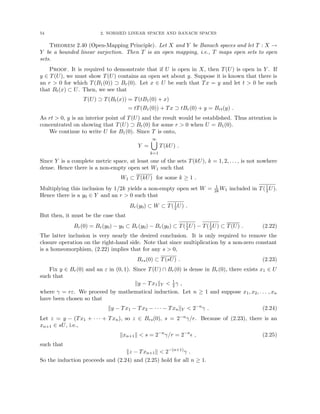
57. 2.7. UNIFORM BOUNDEDNESS PRINCIPLE 57
2.7. Uniform Boundedness Principle
The third basic result in Banach space theory is the Banach-Steinhauss Theorem, also known
as the Principle of Uniform Boundedness.
Theorem 2.45 (Uniform Boundedness Principle). Let X be a Banach space, Y a NLS and
{Tα}α∈I ⊂ B(X, Y ) a collection of bounded linear operators from X to Y . Then one of the
following two conclusions must obtain: either
(a) there is a constant M such that for all α ∈ I,
kTαkB(X,Y ) ≤ M ,
i.e., the Tα are uniformly bounded, or
(b) there is an x ∈ X such that
sup
α∈I
kTαxk = +∞ ,
i.e., there is a single fixed x ∈ X at which the Tαx are unbounded.
Proof. Define the function ϕ : X → [0, ∞] by
ϕ(x) = sup
α∈I
kTαxk ,
for x ∈ X. For n = 1, 2, 3, . . . , let
Vn = {x ∈ X : ϕ(x) n} .
For each α ∈ I, the map ϕα defined by
ϕα(x) = kTαxk
is continuous on X since it is the composition of two continuous maps. Thus the sets
{x : kTαxk n} = ϕ−1
α ((n, ∞))
are open, and consequently,
Vn =
[
α∈I
ϕ−1
α ((n, ∞))
is a union of open sets, so is itself open. Each Vn is either dense in X or it is not. If for some
N, VN is not dense in X, then there is an r 0 and an x0 ∈ X such that
Br(x0) ∩ VN = ∅ .
Therefore, if x ∈ Br(x0), then ϕ(x) ≤ N; thus, if kzk r, then for all α ∈ I,
kTα(x0 + z)k ≤ N .
Hence if kzk r, then for all α ∈ I,
kTα(z)k ≤ kTα(z + x0)k + kTα(x0)k ≤ N + kTαx0k ≤ 2N .
In consequence, we have
sup
α∈I
kTαk ≤
4N
r
,
and so condition (a) holds.
On the other hand, if all the Vn are dense, then they are all dense and open. By Baire’s
Theorem,
∞
n=1
Vn

58. 58 2. NORMED LINEAR SPACES AND BANACH SPACES
is non-empty. Let x ∈
T∞
n=1 Vn. Then, for all n = 1, 2, 3, . . . , ϕ(x) n, and so it follows that
ϕ(x) = +∞.
2.8. Compactness and Weak Convergence in a NLS
In a metric space, an infinite sequence within a compact set always has a convergent subse-
quence. It is therefore useful to characterize compact sets. However, compact sets in a NLS tend
to be quite small. Fortunately, we can define weaker topologies, and thus larger compact sets
and weaker notions of sequential convergence than the one induced by the norm. Some natural
weaker topologies play an interesting and helpful role in numerical analysis and the theory of
partial differential equations.
2.8.1. The norm or strong topology. We begin our study of compactness by noting that
the Heine-Borel theorem is not true in infinite dimensions. That is, a closed and norm-bounded
set with nonempty interior is not compact. First, although we do not have any well-defined
notion of angle in a NLS, we can yet find a point that is nearly orthogonal to a subspace.
Theorem 2.46. Let X be a NLS, Y a closed subspace, and Z a subspace containing Y . If
Z 6= Y and 0 θ 1, then there is some z ∈ Z such that kzk = 1 and
dist(z, Y ) ≥ θ .
Proof. Let z0 ∈ Z Y , and define
d = dist(z0, Y ) = inf
y∈Y
kz0 − yk .
Since Y is closed, d 0, so we can find y0 ∈ Y such that
d
θ
≥ kz0 − y0k ≥ d ,
and set
z =
z0 − y0
kz0 − y0k
∈ Z .
Then, for y ∈ Y ,
kz − yk =
z0 − y0 − ykz0 − y0k
kz0 − y0k
=
kz0 − y1k
kz0 − y0k
≥ kz0 − y1k
θ
d
≥ θ ,
since y1 = y0 + ykz0 − y0k ∈ Y , Y being a subspace.
Corollary 2.47. If X is an infinite dimensional NLS and M is a closed bounded set with
nonempty interior, then M is not compact.
Proof. It is enough to show the result for the closed unit ball. Let x1 ∈ X have norm 1.
By induction, we define a sequence x1, x2, ... , xn such that each has norm 1 and
kxi − xjk ≥ 1/2
for i, j ≤ n and i 6= j. We then continue the induction as follows. Let Y = span{x1, x2, ..., xn}
and choose any x ∈ X Y , which is nonempty since X has infinite dimensions. With Z =
span{Y, x} and θ = 1/2, the previous theorem gives xn+1 ∈ Z of size 1 and such that
dist(xn+1, Y ) ≥ 1/2 .
Thus we have constructed an infinite sequence of points that are at least a distance 1/2
apart from each other. There is clearly has no convergent subsequence, and so we conclude that
the closed unit ball cannot be compact.

59. 2.8. COMPACTNESS AND WEAK CONVERGENCE IN A NLS 59
2.8.2. The weak and weak-∗ topologies. We now define a weaker notion of convergence
than norm convergence.
Definition. Let X be a NLS and {xn}∞
n=1 a sequence in X. We say that {xn}∞
n=1 converges
weakly to x ∈ X if
f(xn) → f(x)
for all f ∈ X∗. We write xn * x or xn
w
−
→ for weak convergence. Let {fn}∞
n=1 be a sequence in
X∗ and f ∈ X∗. We say that fn converges weak-∗ if for each x ∈ X
fn(x) → f(x) .
We write fn
w∗
−→ f to indicate weak-∗ convergence.
Proposition 2.48. Let X be a NLS and {xn}∞
n=1 a sequence from X. If {xn}∞
n=1 converges
weakly, then its weak limit is unique and {kxnkX}∞
n=1 is bounded. If {fn}∞
n=1 ⊂ X∗ converges
weak-∗, then its weak-∗ limit is unique. If in addition X is a Banach space, then {kfnkX∗ }∞
n=1
is bounded.
Proof. Suppose xn * x and xn * y. That means that for any f ∈ X∗,
f(xn) −→ f(x)

y
f(y)
as n → ∞. Consequently f(x) = f(y) for all f ∈ X∗, which means x = y by the Hahn-Banach
Theorem.
Fix an f ∈ X∗. Then the sequence {f(xn)}∞
n=1 is bounded in F, say
|f(xn)| ≤ Cf for all n
since {f(xn)}∞
n=1 converges. View xn as the evaluation map Exn ∈ X∗∗. In this context, the
last condition amounts to
|Exn (f)| ≤ Cf
for all n. Thus we have a collection of bounded linear maps {Exn }∞
n=1 in X∗∗ = B(X∗, F) which
are bounded at each point of their domain X∗. By the Uniform Boundedness Principle, which
can be applied since X∗ is a Banach space, we must have
sup
n
kExn kX∗∗ ≤ C .
But by the Hahn-Banach Theorem,
kExn kX∗∗ = kxnkX .
The conclusions for weak-∗ convergence are left to the reader.
Proposition 2.49. Let X be a NLS and {xn}∞
n=1 ⊂ X. If xn
w
* x, then kxk ≤ lim inf
n→∞
kxnk.
We leave this as an exercise; the result follows from the Hahn-Banach Theorem.
We have actually defined new topologies on X and X∗ by these notions of weak convergence.
Definition. Suppose X is a NLS with dual X∗. The weak topology on X is the smallest
topology on X such that each f ∈ X∗ is continuous. The weak-∗ topology on X∗ is the smallest
topology on X∗ making continuous each evaluation map Ex : X∗ → F, x ∈ X (defined by
Ex(f) = f(x)).

60. 60 2. NORMED LINEAR SPACES AND BANACH SPACES
It is not difficult to describe a base for these topologies. A basic open set containing zero in
the weak topology of X is of the form
U = {x ∈ X : |fi(x)| εi, i = 1, . . . , n} =
n
i=1
f−1
i (Bεi (0))
for some n, εi 0, and fi ∈ X∗, where Bi (0) = {z ∈ F : |z| i}. Similarly for the weak-∗
topology of X∗, a basic open set containing zero is of the form
V = {f ∈ X∗
: |f(xi)| εi, i = 1, . . . , n} =
n
i=1
E−1
xi
(Bεi (0))
for some n, εi 0, and xi ∈ X. The rest of the topology is given by translations and unions of
these. If X is infinite dimensional, these topologies are not compatible with any metric, so some
care is warranted. That our limit processes arise from these topologies is given by the following.
Proposition 2.50. Suppose X is a NLS with dual X∗. Let x ∈ X and {xn}∞
n=1 ⊂ X. Then
xn converges to x in the weak topology if and only if xn
w
* x (i.e., f(xn) → f(x) in F for every
f ∈ X∗). Moreover, if f ∈ X∗ and {fn}∞
n=1 ⊂ X∗, then fn converges to f in the weak-∗ topology
if and only if fn
w∗
−→ f (i.e., fn(x) → f(x) in F for every x ∈ X).
Proof. If xn converges to x in the weak topology, then, since f ∈ X∗ is continuous in the
weak topology (by definition), f(xn) → f(x). That is xn
w
* x. Conversely, suppose f(xn) →
f(x) ∀ f ∈ X∗. Let U be a basic open set containing x. Then
U = x + {y ∈ X : |fi(y)| εi, i = 1, . . . , m}
for some m, εi 0, and fi ∈ X∗. Now there is some N 0 such that
|fi(xn) − fi(x)| = |fi(xn − x)| εi
for all n ≥ N, since fi(xn) → fi(x), so xn = x + (xn − x) ∈ U. That is, x converges to xn in the
weak topology. Similar reasoning gives the result for weak-∗ convergence.
By Proposition 2.48, the weak and weak-∗ topologies are Hausdorff. Obviously the weak
topology on X is weaker than the strong or norm topology (for which more than just the linear
functions are continuous).
On X∗, we have three topologies, the weak-∗ topology (weakest for which the evaluation
maps ⊂ X∗∗ are continuous), the weak topology (weakest for which X∗∗ maps are continuous),
and the strong or norm topology. The weak-∗ topology is weaker than the weak topology, which
is weaker than the strong topology. Of course, if X is reflexive, the weak-∗ and weak topologies
agree.
It is easier to obtain convergence in weaker topologies, as then there are fewer open sets to
consider. In infinite dimensions, the unit ball is not a compact set. However, if we restrict the
open sets in a cover to weakly open sets, we might hope to obtain compactness. This is in fact
the case in X∗.
Theorem 2.51 (Banach-Alaoglu Theorem). Suppose X is a NLS with dual X∗, and B∗
1 is
the closed unit ball in X∗ (i.e., B∗
1 = {f ∈ X∗ : kfk ≤ 1}. Then B∗
1 is compact in the weak-∗
topology.
By a scaling argument, we can immediately generalize the theorem to show that a closed
unit ball of any radius r 0 is weak-∗ compact.

61. 2.8. COMPACTNESS AND WEAK CONVERGENCE IN A NLS 61
Proof. For each x ∈ X, let
Bx = {λ ∈ F : |λ| ≤ kxk} .
Each Bx is closed and bounded in F, and so is compact. By Tychonoff’s Theorem,
C = ×
x∈X
Bx
is also compact. An element of C can be viewed as a function g : X → F satisfying |g(x)| ≤ kxk.
In this way, B∗
1 is the subset of C consisting of the linear functions. The product topology on C
is the weakest one making all coordinate projection maps g 7→ g(x) continuous. As these maps
are the evaluation maps, the inherited topology on B∗
1 is precisely the weak-∗ topology.
Since C is compact, we can complete the proof by showing that B∗
1 is closed in C. Since
X∗ is not a metric space when endowed with the weak-∗ topology, we must show that any
accumulation point g of B∗
1 is in B∗
1, i.e., linear with norm at most one. Fix x, y ∈ X and λ ∈ F.
Since g is an accumulation point, every neighborhood of the form
U = g + {h ∈ C : |h(xi)| εi, i = 1, . . . , m}
intersects B∗
1. Given ε 0, there is a neighborhood with m = 4 containing f ∈ B∗
1 such that
f = g + h ,
where
|h(x)|
ε
3 max(1, |λ|)
, |h(y)|
ε
3
, |h(x + y)|
ε
3
, and |h(λx)|
2
3
.
Thus, since f is linear,
|g(x + y) − g(x) − g(y)| = |h(x + y) − h(x) − h(y)| ≤ ε
and
|g(λx) − λg(x)| = |h(λx) − λh(x)| ≤ ε .
As ε is arbitrary, g is linear. Moreover,
|g(x)| = |f(x) − h(x)| ≤ |f(x)| +
ε
3
≤ kxk +
ε
3
,
so also |g(x)| ≤ kxk. That is, g ∈ B∗
1, so B∗
1 is closed.
What does compactness say about sequences? If the space is metrizable (i.e., there is a metric
that gives the same topology), a sequence in a compact space has a convergent subsequence (see
Proposition 1.27). This is the content of the next theorem.
Theorem 2.52. If X is a separable Banach space and K ⊂ X∗ is weak-∗ compact, then K
is metrizable in the weak-∗ topology.
Proof. Recall that separability means that we can find a dense subset D = {xn}∞
n=1 ⊂ X.
The evaluation maps En : X∗ → F, defined by En(x∗) = x∗(xn), are weak-∗ continuous by
definition. If En(x∗) = En(y∗) for each n, then x∗ and y∗ are two continuous functions that
agree on the dense set D, and so they must agree everywhere. That is, the set {En}∞
n=1 is a
countable set of continuous functions that separates points on X∗.
Now let Cn = supx∗∈K |En(x∗)| ∞, since K is compact and En is continuous, and define
fn = En/Cn. Then |fn| ≤ 1, and
d(x∗
, y∗
) =
∞
X
n=1
2−n
|fn(x∗
) − fn(y∗
)|

62. 62 2. NORMED LINEAR SPACES AND BANACH SPACES
is a metric on K, since the fn separate points.
We now have two topologies, the weak-∗ open sets τ, and the open sets τd generated from
the metric, which we must show coincide. First we show that τd ⊂ τ. For N ≥ 1, let
dN (x∗
, y∗
) =
N
X
n=1
2−n
|fn(x∗
) − fn(y∗
)| ,
which gives the τ-continuous function dN (·, y∗) for fixed y∗. Since dN (·, y∗) converges uniformly
to d(·, y∗), we conclude that d(·, y∗) is also τ-continuous. Finally, any ball Br(y∗) = {x∗ ∈ K :
d(x∗, y∗) r} is the inverse image of the open set (−∞, r), and so is τ-open.
To show the opposite inclusion, τ ⊂ τd, let A ∈ τ. Then Ac ⊂ K is τ-closed, and thus
τ-compact (Proposition 1.24). But τd ⊂ τ implies that Ac is also τd-compact by definition, since
any τd-open cover of Ac is also a τ-open cover, which has a finite subcover. Proposition 1.24
now implies that Ac is τd-closed, and thus A ∈ τd. The proof is complete.
Corollary 2.53. If X is a separable Banach space, {fn}∞
n=1 ⊂ X∗, and there is some R 0
such that kfnk ≤ R for all n, then there is a subsequence {fni }∞
i=1 that converges weak-∗ in X∗.
Corollary 2.54. If Banach space X is separable and reflexive and {xn}∞
n=1 ⊂ X is a
bounded sequence, then there is a subsequence {xn}∞
i=1 that converges weakly in X.
Example. If 1 p ∞ and Ω ∈ Rd is measurable, the Lp(Ω) is separable and reflexive, so a
bounded sequence {fn}∞
n=1 always has a weakly convergent subsequence. That is, if kfnkp ≤ M
for some M 0, then there is some f ∈ Lp(Ω) and subsequence such that fnk
w
* f in Lp(Ω).
Corollary 2.55 (Generalized Heine-Borel Theorem). Suppose X is a Banach space with
dual X∗, and K ⊂ X∗. Then K is weak-∗ compact if and only if K is weak-∗ closed and bounded.
Proof. Any (weak-∗) closed and bounded set K is compact, as it sits in a large closed ball,
which is compact. Conversely, if K is compact, it is closed. It must be bounded, for otherwise
we can find a nonconvergent sequence in K (every weak-∗ convergent sequence is bounded).
We close this section with an interesting result that relates weak and strong convergence.
Theorem 2.56 (Banach-Saks). Suppose that X is a NLS and {xn}∞
n=1 is a sequence in X
that converges weakly to x ∈ X. Then for every n ≥ 1, there are constants αn
j ≥ 0,
n
X
j=1
αn
j = 1,
such that yn =
n
X
j=1
αn
j xj converges strongly to x.
That is, whenever xn
w
* x, there is a sequence yn of finite, convex, linear combinations of
the xn such that yn → x.
Proof. Let zn = xn − x1 and z = x − x1, so that z1 = 0 is in the sequence and zn
w
* z. Let
M =
n
X
j=1
αn
j yj : n ≥ 1, αn
j ≥ 0, and
n
X
j=1
αn
j ≤ 1
,
which is convex. The conclusion of the theorem is that z is in M̄, the (norm) closure of M.
Suppose that this is not the case. Then we can apply the Separating Hyperplane Theorem 2.36
to the closed set M̄ and the compact set {z} to obtain a continuous linear functional f and a

63. 2.9. THE DUAL OF AN OPERATOR 63
number γ such that f(zn) γ but f(z) γ. Thus lim supn→∞ f(zn) ≤ γ, so f(zn) 6→ f(z), and
we have a contradiction to zn
w
* z and must conclude that z ∈ M̄ as required.
Corollary 2.57. Suppose that X is a NLS, and S ⊂ X is convex. Then the weak and
strong (norm) closures of S are identical.
Proof. Let S̄w denote the weak closure, and S̄ the usual norm closure. The Banach-Saks
Theorem implies that S̄w ⊂ S̄, since S is convex. But trivially S̄ ⊂ S̄w.
2.9. The Dual of an Operator
Suppose X and Y are NLS’s and T ∈ B(X, Y ). The operator T induces an operator
T∗
: Y ∗
→ X∗
,
called the dual, conjugate, or adjoint of T, as follows. Let g ∈ Y ∗ and define T∗ : X∗ → F by
the formula
(T∗
g)(x) = g(Tx)
for x ∈ X. Then, T∗g ∈ X∗, for T∗g = g ◦ T is a composition of continuous linear maps,
T g
- -
X Y F
T∗g
and so is itself continuous and linear. Moreover, if g ∈ Y ∗, x ∈ X, then
|T∗
g(x)| = |g(Tx)| ≤ kgkY ∗ kTxkY
≤ kgkY ∗ kTkB(X,Y )kxkX
=
kgkY ∗ kTkB(X,Y )
kxkX .
Hence, not only is T∗g bounded, but
kT∗
gkX∗ ≤ kTkB(X,Y )kgkY ∗ . (2.26)
Thus we have defined a map T∗ : Y ∗ → X∗. In fact, T∗ is itself a bounded linear map,
which is to say T∗ ∈ B(Y ∗, X∗). For linearity, we need to show that for g, h ∈ Y ∗, λ ∈ F,
T∗
(g + h) = T∗
g + T∗
h ,
T∗
(λg) = λT∗
g .
(2.27)
Let x ∈ X and evaluate both sides of these potential equalities at x, viz.
T∗
(g + h)(x) = (g + h)(Tx) = g(Tx) + h(Tx) = T∗
(g)(x) + T∗
h(x) = (T∗
g(g) + T∗
(h))(x)
and
T∗
(λg)(x) = (λg)(Tx) = λg(Tx) = λT∗
g(x) .
As x ∈ X, was arbitrary, it follows that the formulas (2.27) are valid. Thus T∗ is linear. The
fact that T∗ is bounded follows from (2.26), and, moreover,
kT∗
kB(Y ∗,X∗) ≤ kTkB(X,Y ) . (2.28)

64. 64 2. NORMED LINEAR SPACES AND BANACH SPACES
In fact, equality always holds in the last inequality. To see this, first note that if T = 0 is the zero
operator, then T∗ = 0 also and so their norms certainly agree. If T 6= 0, then kTkB(X,Y ) 0.
Let ε 0 be given and let x0 ∈ X, kx0kX = 1 be such that
kTx0kY ≥ kTkB(X,Y ) − ε .
Let g0 ∈ Y ∗ be such that kg0kY ∗ = 1 and
g0(Tx0) = kTx0k .
Such a g0 exists by one of the corollaries of the Hahn-Banach Theorem. Then, it transpires that
kT∗
kB(Y ∗,X∗) ≥ kT∗
g0kX∗ = sup
kxkX =1
|T∗
g0(x)|
≥ |T∗
g0(x0)| = g0(Tx0) = kTx0kY
≥ kTkB(X,Y ) − ε .
In consequence of these ruminations, it is seen that
kT∗
kB(Y ∗,X∗) ≥ kTkB(X,Y ) − ε ,
and ε 0 was arbitrary. Hence
kT∗
kB(Y ∗,X∗) ≥ kTkB(X,Y )
and, along with (2.28), this establishes the result.
The map T 7−→ T∗ itself,
∗ : B(X, Y ) −→ B(Y ∗
, X∗
) ,
has many simple properties of its own, which we leave to the reader to verify.
Proposition 2.58. Let X, Y , and Z be NLS’s, S, T ∈ B(X, Y ), R ∈ B(Y, Z) and λ, µ ∈ F.
Then
(a) kT∗
kB(Y ∗,X∗) = kTkB(X,Y ) (i.e., ∗ is norm preserving) ,
(b) (λT + µS)∗
= λT∗
+ µS∗
(i.e., ∗ is a linear map) ,
(c) (RS)∗
= S∗
R∗
,
(d) (IX)∗
= IX∗ ,
where IX ∈ B(X, X) is the identity mapping of X to itself.
Examples. (a) X = Rd, T : X → X may be represented by a d × d matrix MT in the
standard basis, say. Then T∗ also has a matrix representation in the dual basis and MT∗ = Mt
T
the transpose of MT .
(b) Here is a less elementary, but related example. Let 1 p ∞ and, for f ∈ Lp(0, 1) and
x ∈ (0, 1), set
Tf(x) =
Z 1
0
K(x, y)f(y) dy ,
where K is, say, a bounded measurable function. It is easily determined that T is a bounded
linear map of Lp(0, 1) into itself. We have seen that the dual space of Lp(0, 1) may be realized
concretely as Lq(0, 1), where 1/p + 1/q = 1. That is, for g ∈ Lq(0, 1), Λg ∈ L∗
p(0, 1) is given by
Λg(f) =
Z 1
0
f(x)g(x) dx ,

65. 2.9. THE DUAL OF AN OPERATOR 65
where f ∈ Lp(0, 1). To understand T∗, we compute its action:
(T∗
Λg)(f) = Λg(Tf)
=
Z 1
0
g(x)Tf(x) dx =
Z 1
0
g(x)
Z 1
0
K(x, y)f(y) dy dx
=
Z 1
0
f(y)
Z 1
0
K(x, y)g(x) dx dy .
Now T∗ : L∗
p(0, 1) → L∗
p(0, 1), which can be viewed as T∗ : Lq(0, 1) → Lq(0, 1). Thus, it is
determined that for y ∈ (0, 1),
T∗
(g)(y) =
Z 1
0
K(x, y)g(x) dx .
Lemma 2.59. Let X, Y be NLS’s and T ∈ B(X, Y ). Then T∗∗ : X∗∗ → Y ∗∗ is a bounded
linear extension of T. If X is reflexive, then T = T∗∗.
Proof. Let x ∈ X and g ∈ Y ∗. Realize x as Ex ∈ X∗∗. Then, by definition,
(T∗∗
Ex)(g) = Ex(T∗
g) = T∗
g(x) = g(Tx) = ETx(g) ,
and so
T∗∗
Ex = ETx .
Thus T∗∗|X = T . If X = X∗∗, then this means T = T∗∗.
Lemma 2.60. Let X be a Banach space, Y a NLS and T ∈ B(X, Y ). Then T has a bounded
inverse defined on all of Y if and only if T∗ has a bounded inverse defined on all of X∗. When
either exists, then
(T−1
)∗
= (T∗
)−1
.
Proof. If S = T−1 ∈ B(Y, X), then
S∗
T∗
= (TS)∗
= (IY )∗
= IY ∗ .
This shows that T∗ is one-to-one. The other way around,
T∗
S∗
= (ST)∗
= (TX)∗
= IX∗ ,
shows T∗ is onto. Moreover, S∗ is the inverse of T∗, and of course S∗ is bounded since it is the
dual of a bounded map.
Conversely, if T∗ ∈ B(Y ∗, X∗) has a bounded inverse, then applying the preceding argument,
we ascertain that (T∗∗)−1 ∈ B(Y ∗∗, X∗∗). But,
T∗∗
X
= T ,
so T must be one-to-one. We claim that T maps onto. If so, the Open Mapping Theorem implies
that the inverse is bounded, and we are done. Since T∗∗ is onto, it is an open mapping, and so
T∗∗ takes a closed set to a closed set. Since X is Banach, it is closed, so T∗∗(X) is closed in
Y ∗∗, which is to say that T(X) is closed in Y ∗∗, and hence in Y . Now suppose T is not onto.
Then we can find a y ∈ Y r T(X). By the Hahn-Banach Theorem, since T(X) is closed, there
is a y∗ ∈ Y ∗ such that
y∗
T(X)
= 0 , but y∗
(y) 6= 0 .
But then, for all x ∈ X,
T∗
y∗
(x) = y∗
(Tx) = 0 ,

66. 66 2. NORMED LINEAR SPACES AND BANACH SPACES
whence T∗y∗ = 0, and y∗ = 0, since T∗ is one-to-one. But y∗ 6= 0 in Y ∗, and so we have our
contradiction, and T maps onto Y .
2.10. Exercises
1. Suppose that X is a vector space.
(a) If A, B ⊂ X are convex, show that A + B and A ∩ B are convex. What about A ∪ B and
A B?
(b) Show that 2A ⊂ A + A. When is it true that 2A = A + A?
2. Let (X, d) be a metric space.
(a) Show that
ρ(x, y) = min(1, d(x, y))
is also a metric.
(b) Show that U ⊂ X is open in (X, d) if and only if U is open in (X, ρ).
(c) Repeat the above for
σ(x, y) =
d(x, y)
1 + d(x, y)
.
3. Let X be a NLS, x0 be a fixed vector in X, and α 6= 0 a fixed scalar. Show that the mappings
x 7→ x + x0 and x 7→ αx are homeomorphisms of X onto itself.
4. Show that if X is a NLS, then X is homeomorphic to Br(0) for fixed r. [Hint: consider the
mapping x 7→
xr
1 + kxk
.]
5. In Rd, show that any two norms are equivalent. Hint: Consider the unit sphere, which is
compact.
6. Let X and Y be NLS over the same field, both having the same finite dimension n. Then
prove that X and Y are topologically isomorphic, where a topological isomorphism is defined
to be a mapping that is simultaneously an isomorphism and a homeomorphism.
7. Show that C([a, b]), | · |
, the set of real-valued continuous functions in the interval [a, b]
with the sup-norm (L∞-norm), is a Banach space.
8. If f ∈ Lp(Ω) show that
kfkp = sup
Z
Ω
f g dx = sup
Z
Ω
|f g| dx
where the supremum is taken over all g ∈ Lq(Ω) such that kgkq ≤ 1 and 1/p + 1/q = 1,
where 1 ≤ p, q ≤ ∞.
9. Suppose that Ω ⊂ Rd has finite measure and 1 ≤ p ≤ q ≤ ∞.
(a) Prove that if f ∈ Lq(Ω), then f ∈ Lp(Ω) and
kfkp ≤ (µ(Ω))1/p−1/q
kfkq .
(b) Prove that if f ∈ L∞(Ω), then
lim
p→∞
kfkp = kfk∞ .

67. 2.10. EXERCISES 67
(c) Prove that if f ∈ Lp(Ω) for all 1 ≤ p ∞, and there is K 0 such that kfkp ≤ K, then
f ∈ L∞(Ω) and kfk∞ ≤ K.
10. Finite dimensional matrices.
(a) Let Mn×m be the set of matrices with real valued coefficients aij, for 1 ≤ i ≤ n and
1 ≤ j ≤ m. For every A ∈ Mn×m, define
kAk = max
x∈Rm
|Ax|Rn
|x|Rm
.
Show that Mn×m, k · k
is a NLS.
(b) Each A ∈ Mn×n defines a linear map of Rn into itself. Show that
kAk = max
|x|=|y|=1
yT
Ax ,
where yT is the transpose of y.
(c) Show that each A ∈ Mn×n is continuous.
(d) Prove that the convex hull is convex, and that it is the intersection of all convex subsets
of X containing A.
(e) If X is a normed linear space, prove that the convex hull of an open set is open.
(f) If X is a normed linear space, is the convex hull of a closed set always closed?
(g) Prove that if X is a normed linear space, then the convex hull of a bounded set is
bounded.
11. Prove that if X is a normed linear space and B = B1(0) is the unit ball, then X is infi-
nite dimensional if and only if B contains an infinite collection of non-overlapping balls of
diameter 1/2.
12. Prove that a subset A of a metric space (X, d) is bounded if and only if every countable
subset of A is bounded.
13. Consider (`p, | · |p).
(a) Prove that `p is a Banach space for 1 ≤ p ≤ ∞. Hint: Use that R is complete.
(b) Show that | · |p is not a norm for 0 p 1. Hint: First show the result on R2.
14. If an infinite dimensional vector space X is also a NLS and contains a sequence {en}∞
n=1
with the property that for every x ∈ X there is a unique sequence of scalars {αn}∞
n=1 such
that
kx − (α1e1 + ... + αnen)k → 0 as n → ∞ ,
then {en}∞
n=1 is called a Schauder basis for X, and we have the expansion of x
x =
∞
X
n=1
αnen .
(a) Find a Schauder basis for `p, 1 ≤ p ∞.
(b) Show that if a NLS has a Schauder basis, then it is separable. [Remark: The converse is
not true.]

68. 68 2. NORMED LINEAR SPACES AND BANACH SPACES
15. Let Y be a subspace of a vector space X. The coset of an element x ∈ X with respect to Y
is denoted by x + Y and is defined to be the set
x + Y = {z ∈ X : z = x + y for some y ∈ Y } .
Show that the distinct cosets form a partition of X. Show that under algebraic operations
defined by
(x1 + Y ) + (x2 + Y ) = (x1 + x2) + Y and λ(x + Y ) = λx + Y ,
for any x1, x2, x ∈ X and λ in the field, these cosets form a vector space. This space is called
the quotient space of X by (or modulo Y , and it is denoted X/Y .
16. Let Y be a closed subspace of a NLS X. Show that a norm on the quotient space X/Y is
given for x̂ ∈ X/Y by
kx̂kX/Y = inf
x∈x̂
kxkX .
17. If X and Y are NLS, then the product space X × Y is also a NLS with any of the norms
k(x, y)kX×Y = max(kxkX, kykY )
or, for any 1 ≤ p ∞,
k(x, y)kX×Y = (kxkp
X + kykp
Y )1/p
.
Why are these norms equivalent?
18. If X and Y are Banach spaces, prove that X × Y is a Banach space.
19. Let T : C([0, 1]) → C([0, 1]) be defined by
y(t) =
Z t
0
x(τ) dτ .
Find the range R(T) of T, and show that T is invertible on its range, T−1 : R(T) → C([0, 1]).
Is T−1 linear and bounded?
20. Show that on C([a, b]), for any y ∈ C([a, b]) and scalars α and β, the functionals
f1(x) =
Z b
a
x(t) y(t) dt and f2(x) = αx(a) + βx(b)
are linear and bounded.
21. Find the norm of the linear functional f defined on C([−1, 1]) by
f(x) =
Z 0
−1
x(t) dt −
Z 1
0
x(t) dt .
22. Recall that f = {{xn}∞
n=1 : only finitely many xn 6= 0} is a NLS with the sup-norm |{xn}| =
supn |xn|. Let T : f → f be defined by
T({xn}∞
n=1) = {nxn}∞
n=1 .
Show that T is linear but not continuous (i.e., not bounded).
23. The space C1([a, b]) is the NLS of all continuously differentiable functions defined on [a, b]
with the norm
kxk = sup
t∈[a,b]
|x(t)| + sup
t∈[a,b]
|x0
(t)| .

69. 2.10. EXERCISES 69
(a) Show that k · k is indeed a norm.
(b) Show that f(x) = x0 (a + b)/2
defines a continuous linear functional on C1([a, b]).
(c) Show that f defined above is not bounded on the subspace of C([a, b]) consisting of all
continuously differentiable functions with the norm inherited from C([a, b]).
24. Suppose X is a vector space. The algebraic dual of X is the set of all linear functionals
on X, and is also a vector space. Suppose also that X is a NLS. Show that X has finite
dimension if and only if the algebraic dual and the dual space X∗ coincide.
25. Let X be a NLS and M a nonempty subset. The annihilator Ma of M is defined to be the
set of all bounded linear functionals f ∈ X∗ such that f restricted to M is zero. Show that
Ma is a closed subspace of X∗. What are Xa and {0}a?
26. Define the operator T by the formula
T(f)(x) =
Z b
a
K(x, y) f(y) dy .
Suppose that K ∈ Lq([a, b] × [a, b]), where q lies in the range 1 ≤ q ≤ ∞. Determine the
values of p for which T is necessarily a bounded linear operator from Lp(a, b) to Lq(a, b).
In particular, if a and b are both finite, show that K ∈ L∞([a, b] × [a, b]) implies T to be
bounded on all the Lp-spaces.
27. Let U = Br(0) = {x : kxk r} be an open ball about 0 in a real normed linear space, and
let y 6∈ Ū. Show that there is a bounded linear functional f that separates U from y. (That
is, U and y lie in opposite half spaces determined by f, which is to say there is an α such
that U lies in {x : f(x) α} and f(y) α.)
28. Prove that L2([0, 1]) is of the first category in L1([0, 1]). (Recall that a set is of first category
if it is a countable union of nowhere dense sets, and that a set is nowhere dense if its closure
has an empty interior.) Hint: Show that Ak = {f : kfkL2 ≤ k} is closed in L1 but has empty
interior.
29. If a Banach space X is reflexive, show that X∗ is also reflexive. (∗) Is the converse true?
Give a proof or a counterexample.
30. Let y = (y1, y2, y3, ...) ∈ C∞ be a vector of complex numbers such that
P∞
i=1 yixi converges
for every x = (x1, x2, x3, ...) ∈ C0, where C0 = {x ∈ C∞ : xi → 0 as i → ∞}. Prove that
∞
X
i=1
|yi| ∞ .
31. Let X and Y be normed linear spaces, T ∈ B(X, Y ), and {xn}∞
n=1 ⊂ X. If xn
w
* x, prove
that Txn
w
* Tx in Y . Thus a bounded linear operator is weakly sequentially continuous. Is
a weakly sequentially continuous linear operator necessarily bounded?
32. Suppose that X is a Banach space, M and N are linear subspaces, and that X = M ⊕ N,
which means that
X = M + N = {m + n : m ∈ M, n ∈ N}
and M ∩ N is the trivial linear subspace consisting only of the zero element. Let P denote
the projection of X onto M. That is, if x = m + n, then
P(x) = m

70. 70 2. NORMED LINEAR SPACES AND BANACH SPACES
Show that P is well defined and linear. Prove that P is bounded if and only if both M and
N are closed.
33. Let X be a Banach space, Y a NLS, and Tn ∈ B(X, Y ) such that {Tnx}∞
n=1 is a Cauchy
sequence in Y . Show that {kTnk}∞
n=1 is bounded. If, in addition, Y is a Banach space, show
that if we define T by Tnx → Tx, then T ∈ B(X, Y ).
34. Let X be the normed space of sequences of complex numbers x = {xi}∞
i=1 with only finitely
many nonzero terms and norm defined by kxk = supi |xi|. Let T : X → X be defined by
y = Tx = {x1,
1
2
x2,
1
3
x3, ...} .
Show that T is a bounded linear map, but that T−1 is unbounded. Why does this not
contradict the Open Mapping Theorem?
35. Give an example of a function that is closed but not continuous.
36. For each α ∈ R, let Eα be the set of all continuous functions f on [−1, 1] such that f(0) = α.
Show that the Eα are convex, and that each is dense in L2([−1, 1]).
37. Suppose that X, Y , and Z are Banach spaces and that T : X × Y → Z is bilinear and
continuous. Prove that there is a constant M ∞ such that
kT(x, y)k ≤ Mkxk kyk for all x ∈ X, y ∈ Y .
Is completeness needed here?
38. Prove that a bilinear map is continuous if it is continuous at the origin (0, 0).
39. Consider X = C([a, b]), the continuous functions defined on [a, b] with the maximum norm.
Let {fn}∞
n=1 be a sequence in X and suppose that fn
w
* f. Prove that {fn}∞
n=1 is pointwise
convergent. That is,
fn(x) → f(x) for all x ∈ [a, b] .
Prove that a weakly convergent sequence in C1([a, b]) is convergent in C([a, b]). (∗) Is this
still true when [a, b] is replaced by R?
40. Let X be a normed linear space and Y a closed subspace. Show that Y is weakly sequentially
closed.
41. Let X be a normed linear space. We say that a sequence {xn}∞
n=1 ⊂ X is weakly Cauchy
if {Txn}∞
n=1 is Cauchy for all T ∈ X∗, and we say that X is weakly complete if each weak
Cauchy sequence converges weakly. If X is reflexive, prove that X is weakly complete.
42. Show that every finite dimensional vector space is reflexive.
43. Show that C([0, 1]) is not reflexive.
44. If X and Y are Banach spaces, show that E ⊂ B(X, Y ) is equicontinuous if, and only if,
there is an M ∞ such that kTk ≤ M for all T ∈ E.
45. Let X be a Banach space and T ∈ X∗ = B(X, F). Identify the range of T∗ ∈ B(F, X∗).
46. Let X be a Banach space, S, T ∈ B(X, X), and I be the identity map.
(a) Show by example that ST = I does not imply TS = I.
(b) If T is compact, show that S(I − T) = I if, and only if, (I − T)S = I.
(c) If S = (I − T)−1 exists for some T compact, show that I − S is compact.

71. 2.10. EXERCISES 71
47. Let 1 ≤ p ∞ and define, for each r ∈ Rd, Tr : Lp(Rd) → Lp(Rd) by
Tr(f)(x) = f(x + r) .
(a) Verify that Tr(f) ∈ Lp(Rd) and that Tr is bounded and linear. What is the norm of Tr?
(b) Show that as r → s, kTrf − TsfkLp → 0. Hint: Use that the set of continuous functions
with compact support are dense in Lp(Rd) for p ∞.

73. CHAPTER 3
Hilbert Spaces
The norm of a normed linear space gives a notion of absolute size for the elements of the
space. While this has generated an extremely interesting and useful structure, often one would
like more geometric information about the elements. In this chapter we add to the NLS structure
a notion of “angle” between elements and, in particular, a notion of orthogonality through a
device known as an inner-product.
3.1. Basic Properties of Inner-Products
Definition. An inner-product on a vector space H is a map (·, ·) : H × H → F satisfying
the following properties.
(a) The map (·, ·) is linear in its first argument; that is, for α, β ∈ F and x, y, z ∈ H,
(αx + βy, z) = α(x, z) + β(y, z) .
(b) The map (·, ·) is conjugate symmetric (symmetric if F = R), meaning that for x, y ∈ H,
(x, y) = (y, x) .
(c) For any x ∈ H, (x, x) ≥ 0; moreover, (x, x) = 0 if and only if x = 0.
If H has such an inner-product, then H is called an inner-product space (IPS) or a pre-Hilbert
space. Any map satisfying (a) and (b) is said to be sesquilinear (or bilinear, if F = R). We often
denote the inner-product on H as (·, ·)H or h·, ·iH.
Proposition 3.1. If (·, ·) is sesquilinear on H, then for α, β ∈ F and x, y, z ∈ F,
(x, αy + βz) = α(x, y) + β(x, z) .
That is, (·, ·) is conjugate linear in its second argument.
Examples.
(a) Fd (i.e., Cd or Rd) is an IPS with the inner-product
(x, y) = x · ȳ =
d
X
i=1
xiȳi, x, y ∈ Fd
.
(b) Similarly `2 is an IPS with
(x, y) =
∞
X
i=1
xiȳi , x, y ∈ `2 .
The Hölder inequality shows that this quantity is finite.
(c) For any measurable set Ω ⊂ Rd, L2(Ω) has inner-product
(f, g) =
Z
Ω
f(x) g(x) dx , f, g ∈ L2(Ω) .
73

74. 74 3. HILBERT SPACES
Definition. If (H, (·, ·)) is an IPS, we define the map k · k : H → R by
kxk = (x, x)1/2
for any x ∈ H. This map is called the induced norm.
Lemma 3.2 (Cauchy-Schwarz Inequality). If (H, (·, ·)) is an IPS with induced norm k · k,
then for any x, y ∈ H,
|(x, y)| ≤ kxk kyk ,
with equality holding if and only if x or y is a multiple of the other.
Proof. If y = 0, there is nothing to prove, so assume y 6= 0. Then for x, y ∈ H and λ ∈ F,
0 ≤ kx − λyk2
= (x − λy, x − λy)
= (x, x) − λ(x, y) − λ(y, x) + |λ|2
(y, y)
= kxk2
− ( λ(y, x) + λ(y, x)) + |λ|2
kyk2
= kxk2
− 2 Real(λ(y, x)) + |λ|2
kyk2
.
Let
λ =
(x, y)
kyk2
.
Then
0 ≤ kxk2
− 2 Real
(x, y)(y, x)
kyk2
+
|(x, y)|2
kyk4
kyk2
= kxk2
−
|(x, y)|2
kyk2
,
since (x, y)(y, x) = |(x, y)|2 is real. A rearrangement gives the result, with equality only if
x − λy = 0.
Corollary 3.3. The induced norm is indeed a norm, and thus an IPS is a NLS.
Proof. For α ∈ F and x ∈ H, kxk ≥ 0, kαxk = (αx, αx)1/2 = |α|(x, x)1/2 = |α| kxk and
kxk = 0 if and only if (x, x) = 0 if and only if x = 0.
It remains only to demonstrate the triangle inequality. For x, y ∈ H,
kx + yk2
= (x + y, x + y)
= kxk2
+ 2 Real(x, y) + kyk2
≤ kxk2
+ 2|(x, y)| + kyk2
≤ kxk2
+ 2kxk kyk + kyk2
= (kxk + kyk)2
.
Note that the Cauchy-Schwarz inequality gives a notion of angle, as we may define the angle
θ between x and y from
cos θ =
|(x, y)|
kxk kyk
≤ 1 .
However, generally we consider only the case where θ = π/2.
Definition. If (H, (·, ·)) is an IPS, x, y ∈ H, and (x, y) = 0, then we say that x and y are
orthogonal, and denote this fact as x ⊥ y.

75. 3.2. BEST APPROXIMATION AND ORTHOGONAL PROJECTIONS 75
Proposition 3.4 (Parallelogram Law). If x, y ∈ H, an IPS, then
kx + yk2
+ kx − yk2
= 2(kxk2
+ kyk2
)
Proof. Exercise.
The parallelogram law can be used to show that not all norms come from an inner-product,
as there are norms that violate the law. The law expresses the geometry of a parallelogram in
R2, generalized to an arbitrary IPS.
Lemma 3.5. If (H, h·, ·i) is an IPS, then h·, ·i : H × H → F is continuous.
Proof. Since H×H is a metric space, it is enough to show sequential continuity. So suppose
that (xn, yn) → (x, y) in H × H; that is, both xn → x and yn → y. Then
|hxn, yni − hx, yi| = |hxn, yni − hxn, yi + hxn, yi − hx, yi|
≤ |hxn, yni − hxn, yi| + |hxn, yi − hx, yi|
= |hxn, yn − yi| + |hxn − x, yi|
≤ kxnk kyn − yk + kxn − xk kyk .
Since xn → x, kxnk is bounded. Thus |hxn, yni − hx, yi| can be made as small as desired by
taking n sufficiently large.
Corollary 3.6. If λn → λ and µn → µ in F and xn → x and yn → y in H, then
hλnxn, µnyni → hλx, µyi .
Proof. Just note that λnxn → λx and µnyn → µy.
Definition. A complete IPS H is called a Hilbert space.
Hilbert spaces are thus Banach spaces.
3.2. Best Approximation and Orthogonal Projections
The following is an important geometric relation in an IPS.
Theorem 3.7 (Best approximation). Suppose (H, (·, ·)) is an IPS and M ⊂ H is nonempty,
convex, and complete (e.g,, closed if H is Hilbert). If x ∈ H, then there is a unique y = y(x) ∈ M
such that
dist(x, M) ≡ inf
Z∈M
kx − zk = kx − yk .
We call y the best approximation of or closest point to x from M.
Proof. Let
δ = inf
Z∈M
kx − zk .
If δ = 0, we must take x = y. That y = x is in M follows from completeness, since given any
integer n ≥ 1, there is some zn ∈ M such that kx − znk = 1/n, so zn → x ∈ M.
Suppose δ 0. Then x /
∈ M and so there is a sequence {yn}∞
n=1 ⊂ M such that as n → ∞,
kx − ynk ≡ δn → δ .

76. 76 3. HILBERT SPACES
We claim that {yn} is Cauchy. By the parallelogram law,
kyn − ymk2
= k(yn − x) + (x − ym)k2
= 2 kyn − xk2
+ kx − ymk2
− kyn + ym − 2xk2
= 2(δ2
n + δ2
m) − 4
yn + ym
2
− x
2
≤ 2(δ2
n + δ2
m) − 4δ2
,
since by convexity (yn + ym)/2 ∈ M. Thus as n, m → ∞, kyn − ymk → 0. By completeness,
yn → y for some y ∈ M. Since k · k is continuous, kx − yk = δ.
To see that y is unique, suppose that for some z ∈ M, kx − zk = δ. Then the parallelogram
law again shows
ky − zk2
= k(y − x) + (x − z)k2
= 2 ky − xk2
+ kx − zk2
− ky + z − 2xk2
= 4δ2
− 4
y + z
2
− x
2
≤ 4δ2
− 4δ2
= 0 .
Thus y = z.
Corollary 3.8. Suppose (H, (·, ·)) is an IPS and M is a complete linear subspace. If x ∈ H
and y ∈ M is the best approximation to x in M, then
x − y ⊥ M .
Proof. Let m ∈ M, m 6= 0. For any λ ∈ F, by best approximation,
kx − yk2
≤ kx − y + λmk2
= kx − yk2
+ λ(x − y, m) + λ(m, x − y) + |λ|2
kmk2
With λ = −(x − y, m)/kmk2, we have
0 ≤ −λλkmk2
− λλkmk2
+ |λ|2
kmk2
= −|λ|2
kmk2
,
so λ = 0, which means
(x − y, m) = 0
for any m ∈ M. That is, x − y ⊥ M.
Definition. Given an IPS H and M ⊂ H,
M⊥
= {x ∈ H : (x, m) = 0 ∀ m ∈ M} .
The space M⊥ is referred to as “M-perp.”
Proposition 3.9. Suppose H is an IPS and M ⊂ H. Then M⊥ is a closed linear subspace
of H, M ⊥ M⊥, and M ∩ M⊥ is either {0} or ∅.
Closure follows easily from the continuity of the inner-product.
Theorem 3.10. Suppose (H, (·, ·)) is an IPS and M ⊂ H is a complete linear subspace.
Then there exist two unique bounded linear surjective mappings
P : H → M and P⊥
: H → M⊥
defined for any x ∈ H by
(a) kx − Pxk = infy∈M kx − yk (i.e., Px is the best approximation to x in M),

77. 3.2. BEST APPROXIMATION AND ORTHOGONAL PROJECTIONS 77
(b) x = Px + P⊥x (i.e., P⊥ = I − P),
with the additional properties
(c) kxk2 = kPxk2 + kP⊥xk2,
(d) x ∈ M if and only if P⊥x = 0 (i.e., x = Px),
(e) x ∈ M⊥ if and only if Px = 0 (i.e., x = P⊥x),
(f) kPk = 1 unless M = {0}, and kP⊥k = 1 unless M = H,
(g) PP⊥ = P⊥P = 0, P2 = P, and (P⊥)2 = P⊥ (i.e., P and P⊥ are orthogonal projection
operators),
(h) y = Px if and only if y ∈ M satisfies (x − y, m) = 0 for all m ∈ M.
Note that (c) is the Pythagorean theorem in an IPS, since Px ⊥ P⊥x and (b) holds. We call P
and P⊥ the orthogonal projections of H onto M and M⊥, respectively.
Proof. By the best approximation theorem, (a) defines P uniquely, and then (b) defines
P⊥ : H → H uniquely. But if x ∈ H, then for m ∈ M,
(P⊥
x, m) = (x − Px, m) = 0
by Corollary 3.8, so the range of P⊥ is M⊥.
To see that P and P⊥ are linear, let α, β ∈ F and x, y ∈ H. Then by (b),
αx + βy = P(αx + βy) + P⊥
(αx + βy) ,
and
αx + βy = α(Px + P⊥
x) + β(Py + P⊥
y)
= αPx + βPy + αP⊥
x + βP⊥
y .
Thus
αPx + βPy − P(αx + βy) = P⊥
(αx + βy) − αP⊥
x − βP⊥
y .
Since M and M⊥ are vector spaces, the left side above is in M and the right side is in M⊥. So
both sides are in M ∩ M⊥ = {0}, and so
P(αx + βy) = αPx + βPy ,
P⊥
(αx + βy) = αP⊥
x + βP⊥
y ;
that is, P and P⊥ are linear.
From the proof of the best approximation theorem, we saw that if x ∈ M, then Px = x;
thus, P is surjective. Also, x = Px implies x = Px ∈ M, so (d) follows.
If x ∈ M⊥, then since x = Px + P⊥x,
x − P⊥
x = Px ∈ M ∩ M⊥
= {0} ,
so x ∈ P⊥x, P⊥ is surjective, and (e) follows.
If x ∈ H, then (e) and (d) imply that PP⊥x = 0 since P⊥x ∈ M⊥ and P⊥Px = 0 since
Px ∈ M, so 0 = PP⊥ = P(I − P) = P − P2 and 0 = P⊥P = P⊥(I − P⊥) = P⊥ − (P⊥)2. That
is, (g) follows.
We obtain (c) by direct computation,
kxk2
= kPx + P⊥
xk2
= (Px + P⊥
x, Px + P⊥
x)
= kPxk2
+ (Px, P⊥
x) + (P⊥
x, Px) + kP⊥
xk2
.
The two cross terms on the left vanish since M ⊥ M⊥.

78. 78 3. HILBERT SPACES
Finally, (c) implies that
kPxk2
= kxk2
− kP⊥
xk ≤ kxk2
,
so kPk ≤ 1. But if M 6= {0}, there exists x ∈ M {0} for which kPxk = kxk. Thus kPk = 1.
Similarly remarks apply to P⊥. We conclude that P and P⊥ are bounded and (f) holds.
For (h), Corollary 3.8 gives the forward implication. For the converse, note that kx − (y +
m)k2 = kx − yk2 + kmk2, which is minimized for m = 0. Thus y = Px.
Corollary 3.11. If (H, (·, ·)) is a Hilbert space and M ⊂ H is a closed linear subspace,
then P⊥ is best approximation of H in M⊥.
Proof. We have the unique operators PM and (PM )⊥ from the theorem. Now M⊥ is closed,
so we can apply the theorem also to M⊥ to obtain the unique operators PM⊥ and (PM⊥ )⊥. It
is not difficult to conclude that PM⊥ = (PM )⊥, which is best approximation of H in M⊥.
3.3. The Dual Space
We turn now to a discussion of the dual H∗ of a Hilbert space (H, (·, ·)). We first observe
that if y ∈ H, then the functional Ly defined by
Ly(x) = (x, y)
is linear in x and bounded by the Cauchy-Schwarz inequality. In fact,
|Ly(x)| ≤ kyk kxk ,
so kLyk ≤ kyk. But |Ly(y/kyk)| = kyk, so in fact
kLyk = kyk .
We conclude that Ly ∈ H∗, and, as y is arbitrary,
{Ly}y∈H ⊂ H∗
.
We have represented certain members of H∗ as Ly maps; in fact, as we will see, every member
of H∗ can be so represented. Thus by identifying Ly with y, we see that in some sense H is its
own dual.
Theorem 3.12 (Riesz Representation Theorem). Let (H, (·, ·)) be a Hilbert space and L ∈
H∗. Then there is a unique y ∈ H such that
Lx = (x, y) ∀ x ∈ H .
Moreover, kLkH∗ = kykH.
Proof. If L ≡ 0 (i.e., Lx = 0 ∀ x ∈ H), then take y = 0. Uniqueness is clear, since if
Lx = (x, z), then
0 = Lz = (z, z) = kzk2
implies z = 0.
Suppose then that L 6≡ 0. Let
M = N(L) ≡ ker(L) ≡ {x ∈ H : Lx = 0} .
As M is the inverse image of the closed set {0} under L, M is closed. Easily M is a vector
space, so M is a closed (i.e., complete) linear subspace of H.

79. 3.4. ORTHONORMAL SUBSETS 79
Since L 6≡ 0, M 6= H and M⊥ 6= {0} by Theorem 3.10. Let z ∈ M⊥ {0}, normalized so
kzk = 1. For x ∈ H, let
u = (Lx)z − (Lz)x ,
so
Lu = (Lx)(Lz) − (Lz)(Lx) = 0 .
Thus u ∈ M and so u ⊥ z. That is,
0 = (u, z) =
(Lx)z − (Lz)x, z
= Lx(z, z) − Lz(x, z) = Lx − Lz(x, z) ,
or
Lx = Lz(x, z) = (x, (Lz)z) .
Uniqueness is trivial, for if
Lx = (x, y1) = (x, y2) ∀ x ∈ H ,
then
(x, y1 − y2) = 0 ∀ x ∈ H .
Substitute x = y1 −y2 to conclude y1 = y2. Finally, we already saw that kLk = kLyk = kyk.
We define a map R : H → H∗, called the Riesz map, by
Rx = Lx ∀ x ∈ H .
The Riesz Representation Theorem says that R is one-to-one and onto. Thus we identify H
with its dual precisely through R: Given x ∈ H there is a unique Rx = Lx ∈ H∗, and conversely
given L ∈ H∗, there is a unique x = R−1L ∈ H such that L = Lx. While R is not linear when
F = C, it is conjugate linear:
R(x + y) = Rx + Ry ∀ x, y ∈ H ,
R(λx) = λRx ∀ x ∈ H, λ ∈ F .
3.4. Orthonormal Subsets
In finite dimensions, a vector space is isomorphic to Rd for some d ∞, which can be
described by an orthogonal basis. Similar results hold for infinite dimensional Hilbert spaces.
Definition. Suppose H is an IPS and I is some index set. A set A = {xα}α∈I ⊂ H is said
to be orthogonal if xα 6= 0 ∀ α ∈ I and
xα ⊥ xβ (i.e., (xα, xβ) = 0)
for all α, β ∈ I, α 6= β. Furthermore, if also kxαk = 1 ∀ α ∈ I, then A is orthonormal (ON).
Definition. If A ⊂ X, a NLS, then A is linearly independent if every finite subset of A
is linearly independent. That is, every collection {xi}n
i=1 ⊂ A must satisfy the property that if
there are scalars ci ∈ F with
n
X
i=1
cixi = 0 (3.1)
then necessarily ci = 0 ∀ i.

80. 80 3. HILBERT SPACES
Proposition 3.13. If a subset A of a Hilbert space H is orthogonal, and 0 6∈ A, then A is
linearly independent.
Proof. If {xi}n
i=1 ⊂ A and ci ∈ F satisfy (3.1), then for 1 ≤ j ≤ n,
0 =
n
X
i=1
cixi, xj
=
n
X
i=1
ci(xi, xj) = cjkxjk2
.
As xj 6= 0, necessarily each cj = 0.
Let {x1, . . . , xn} be linearly independent in a Hilbert space H, and
M = span{x1, . . . , xn} ,
which is closed in H as it is finite dimensional. We compute the orthogonal projection of x ∈ H
onto M. That is, we want c1, . . . , cn ∈ F such that PM x =
Pn
j=1 cjxj and PM x − x ⊥ M. That
is, for every 1 ≤ i ≤ n,
(PM x, xi) = (x, xi) .
Now
(PM x, xi) =
n
X
j=1
cj(xj, xi) ,
so with
aij = (xi, xj) and bi = (x, xi)
we have that the n × n matrix A = (aij) and n-vectors b = (bi) and c = (cj) satisfy
Ac = b .
We already know that a unique solution c exists, so A is invertible and the solution c can be
found, giving PM x.
Theorem 3.14. Suppose H is a Hilbert space and {u1, . . . , un} ⊂ H is ON. Let x ∈ H.
Then the orthogonal projection of x onto M = span{u1, . . . , un} is given by
PM x =
n
X
i=1
(x, ui)ui .
Moreover,
n
X
i=1
|(x, ui)|2
≤ kxk2
.
Proof. In this case, the matrix A = ((ui, uj)) = I, so our coefficients c are the values
b = ((x, ui)). The final remark follows from the fact that kPM xk ≤ kxk and the calculation
kPM xk2
=
n
X
i=1
|(x, ui)|2
,
left to the reader.

81. 3.4. ORTHONORMAL SUBSETS 81
We extend this result to larger ON sets. To do so, we need to note a few facts about infinite
series. Let I be any index set (possibly uncountable!), and {xα}α∈I a series of nonnegative real
numbers. We define
X
α∈I
xα = sup
J ⊂I
J finite
X
α∈J
xα .
If I = N = {0, 1, 2, . . . } is countable, this agrees with the usual definition
∞
X
α=0
xα = lim
n→∞
n
X
α=0
xα .
We leave it to the reader to verify that if
X
α∈I
xα ∞ ,
then at most countably many xα are nonzero.
Theorem 3.15 (Bessel’s inequality). Let H be a Hilbert space and {uα}α∈I ⊂ H an ON set.
For x ∈ H,
X
α∈I
|(x, uα)|2
≤ kxk2
.
Proof. By the previous theorem, for any finite J ⊂ I,
X
α∈J
|(x, uα)|2
≤ kxk2
,
so the same is true of the supremum.
Corollary 3.16. At most countably many of the (x, uα) are nonzero.
In a sense to be made precise below in the Riesz-Fischer Theorem, x ∈ H can be associated
to its coefficients (x, uα) ∀ α ∈ I, where I is some index set. The subtlety is that I may be
uncountable. We define a space of coefficients below.
Definition. Let I be a set. We denote by `2(I) the set
`2(I) =
n
f : I → F :
X
α∈I
|f(α)|2
∞
o
.
If I = N, we have the usual space `2, which is a Hilbert space. In general, we have an
inner-product on `2(I) given by
(f, g) =
X
α∈I
f(α)g(α) ,
as the reader can verify. Moreover, `2(I) is complete.
Theorem 3.17 (Riesz-Fischer Theorem). Let H be a Hilbert space and {uα}α∈I any ON set
in H. Define the mapping F : H → `2(I) by F(x) = fx, where
fx(α) = xα ≡ (x, uα) for α ∈ I .
Then F is a surjective, bounded linear map.

82. 82 3. HILBERT SPACES
Proof. Denoting the map fx by {xα}α∈I, the mapping F is linear since
F(x + y) = {(x + y)α}α∈I = {(x + y, uα)}α∈I
= {(x, uα) + (y, uα)}α∈I
= {(x, uα)}α∈I + {(y, uα)}α∈I
= F(x) + F(y) ,
and similarly for scalar multiplication. F is a bounded map because of Bessel’s inequality
kF(x)k2
`2(I) =
X
α∈I
|xα|2
≤ kxk2
H .
Thus, not only is F bounded, but
kFkB(H,`2(I)) ≤ 1 .
The interesting point is that F is surjective. Let f ∈ `2(I) and let n ∈ N. If
In =
n
α ∈ I : |f(α)|
1
n
o
,
then if |In| denotes the number of α in In,
|In| ≤ n2
kfk2
`2(I) .
Let J =
S∞
n=1 In. Then J is countable and if β /
∈ J , then f(β) = 0. In H, define xn by
xn =
X
α∈In
f(α)uα .
Since In is a finite set, xn is a well-defined element of H. We expect that {xn}∞
n=1 is Cauchy in
H. To see this, let n m ≥ 1 and compute
kxn − xmk2
=
X
α∈InrIm
f(α)uα
2
=
X
α∈InrIm
|f(α)|2
≤
X
α∈IrIm
|f(α)|2
and the latter is the tail of an absolutely convergent series, and so is as small as we like provided
we take m large enough. Since H is a Hilbert space, there is an x ∈ H such that xn
H
−
→ x. As
F is continuous, F(xn) → F(x). We show that F(x) = f. By continuity of the inner-product,
for α ∈ I
F(x)(α) = (x, uα) = lim
n→∞
(xn, uα)
= lim
n→∞
X
β∈In
f(β)(uβ, uα) = f(α) .
Theorem 3.18. Let H be a Hilbert space. The following are equivalent conditions on an ON
set {uα}α∈I ⊂ H.
(i) {uα}α∈I is a maximal ON set (also called an ON basis for H).
(ii) Span{uα : α ∈ I} is dense in H.
(iii) kxk2
H =
P
α∈I |(x, uα)|2 for all x ∈ H.
(iv) (x, y) =
P
α∈I(x, uα)(y, uα) for all x, y ∈ H.

83. 3.4. ORTHONORMAL SUBSETS 83
Proof. (i) =⇒ (ii). Let M = span{uα}. Then M is a closed linear subspace of H. If M
is not all of H, M⊥ 6= {0} since H = M + M⊥. Let x ∈ M⊥, x 6= 0, kxk = 1. Then the set
{uα : α ∈ I} ∪ {x} is an ON set, so {uα}α∈I is not maximal, a contradiction.
(ii) =⇒ (iii). We are assuming M = H in the notation of the last paragraph. Let x ∈ H.
Because of Bessel’s inequality,
kxk2
≥
X
α∈I
|xα|2
,
where xα = (x, uα) for α ∈ I. Let ε 0 be given. Since span{uα : α ∈ I} is dense, there is a
finite set α1, . . . , αN and constants c1, . . . , cN such that
x −
N
X
i=1
ciuαi ≤ ε .
By the Best Approximation analysis, on the other hand,
x −
N
X
i=1
xαi uαi ≤ x −
N
X
i=1
ciuαi .
It follows from orthonormality of the {uα}α∈I that
ε2
≥ x −
N
X
i=1
xαi uαi
2
= kxk2
−
N
X
i=1
|xαi |2
≥ kxk2
−
X
α∈I
|xα|2
.
In consequence,
kxk2
≤
X
α∈I
|xα|2
+ ε ,
and ε 0 was arbitrary. Thus equality holds everywhere in Bessel’s inequality.
(iii) =⇒ (iv). This follows because in a Hilbert space, the norm determines the inner-
product as we now show. Let x, y ∈ H. Because of (iii), we have
kxk2
+ kyk2
+ (x, y) + (y, x) = kx + yk2
=
X
α∈I
|xα + yα|2
=
X
α∈I
|xα|2
+
X
α∈I
|yα|2
+
X
α∈I
xαȳα +
X
α∈I
x̄αyα ;
whereas
kxk2
+ kyk2
+ i(y, x) − i(x, y) = kx + iyk2
=
X
α∈I
|xα + iyα|2
=
X
α∈I
|xα|2
+
X
α∈I
|yα|2
+ i
X
α∈I
yαx̄α − i
X
α∈I
xαȳα .
Since
kxk2
=
X
α∈I
|xα|2
and kyk2
=
X
α∈I
|yα|2
,
it is ascertained that
(x, y) + (x, y) =
X
α∈I
xαȳα +
X
α∈I
xαȳα
and
(x, y) − (x, y) =
X
α∈I
xαȳα −
X
α∈I
xαȳα ,
and the desired result follows (even for F = R, in which case the argument above simplifies).

84. 84 3. HILBERT SPACES
(iv) =⇒ (i). If {uα}α∈I is not a maximal ON set, let u ∈ H, u ⊥ uα for all α ∈ I, and
kuk = 1. Then, because of (iv),
1 = kuk2
=
X
α∈I
|(u, uα)|2
= 0 ,
a contradiction.
Corollary 3.19. If {uα}α∈I is maximal ON and x ∈ H is infinite dimensional, then there
are αi ∈ I for i = 1, 2, . . . such that
x =
∞
X
i=1
(x, uαi )uαi =
X
α∈I
(x, uα)uα .
Proof. Exercise.
That is, indeed, a maximal ON set is a type of basis for the Hilbert space. We call (x, uα)
the Fourier coefficients of x in the ON basis {uα}α∈I.
Corollary 3.20. If {uα}α∈I is a maximal ON set, then the Riesz-Fischer map F : H →
`2(I) is a Hilbert space isomorphism.
That F is injective follows, for a linear map, from Fx = 0 implying that x = 0, which follows
from (iii) of Theorem 3.18
Theorem 3.21. Let H be a Hilbert space and {uα}α∈I any ON set in H. Then {uα}α∈I ⊂
{uβ}β∈J where the latter is ON and maximal.
Proof. The general result follows from transfinite induction. We prove the result assuming
that H is also separable.
Let {x̃j}∞
j=1 be dense in H and
M = span{uα}α∈I .
Define
x̂j = x̃j − PM x̃j ∈ M⊥
,
where PM is orthogonal projection onto M. Then the span of
{uα}α∈I ∪ {x̂j}∞
j=1
is dense in H. Define successively for j = 1, 2, . . . (with x1 = x̂1)
Nj = span{x1, . . . , xj} ,
xj+1 = x̂j+1 − PNj x̂j+1 ∈ N⊥
j .
Then the span of
{uα}α∈I ∪ {xj}∞
j=1
is dense in H and any two elements are orthogonal. Remove any zero vectors and normalize to
complete the proof by the equivalence of (ii) and (iii) in Theorem 3.18.
Corollary 3.22. Every Hilbert space H is isomorphic to `2(I) for some I. Moreover, H
is infinite dimensional and separable if and only if H is isomorphic to `2(N).

85. 3.4. ORTHONORMAL SUBSETS 85
We illustrate orthogonality in a Hilbert space by considering Fourier series. If f : R → C
is periodic of period T, then g : R → C defined by g(x) = f(λx) for some λ 6= 0 is periodic of
period T/λ. So when considering periodic functions, it is enough to restrict to the case T = 2π.
Let
L2,per(−π, π) = {f : R → C : f ∈ L2([−π, π)) and f(x + 2nπ) = f(x)
for a.e. x ∈ [−π, π) and integer n} .
With the inner-product
(f, g) =
1
2π
Z π
−π
f(x) g(x) dx ,
L2,per(−π, π) is a Hilbert space (it is left to the reader to verify these assertions). The set
{einx
}∞
n=−∞ ⊂ L2,per(−π, π)
is ON, as can be readily verified.
Theorem 3.23. The set span{einx}∞
n=−∞ is dense in L2,per(−π, π).
Proof. We first remark that Cper([−π, π]), the continuous functions defined on (−∞, ∞)
that are periodic, are dense in L2,per(−π, π). In fact, C0([−π, π]) is dense (Proposition 2.22) and
clearly periodic. Thus it is enough to show that a continuous and periodic function f of period
2π is the limit of functions in span{einx}∞
n=−∞.
For any integer m ≥ 0, on [−π, π] let
km(x) = cm
1 + cos x
2
m
≥ 0
where cm is defined so that
1
2π
Z π
−π
km(x) dx = 1 . (3.2)
As m → ∞, km(x) is concentrated about x = 0 but maintains total integral 2π (i.e., km/2π → δ0,
the Dirac distribution to be defined later). Now
km(x) = cm
2 + eix + e−ix
4
m
∈ span {einx
}m
n=−m ,
and so, for some λn ∈ C,
fm(x) ≡
1
2π
Z π
−π
km(x − y)f(y) dy
=
1
2π
Z π
−π
m
X
n=−m
λnein(x−y)
f(y) dy
=
m
X
n=−m
λn
2π
Z π
−π
e−iny
f(y) dy
einx
∈ span {einx
}m
n=−m .
We claim that in fact fm → f uniformly in the L∞ norm, so also in L2, and the proof will
be complete. By periodicity,
fm(x) =
1
2π
Z π
−π
f(x − y)km(y) dy ,

86. 86 3. HILBERT SPACES
and, by (3.2),
f(x) =
1
2π
Z π
−π
f(x)km(y) dy .
Thus, for any δ 0,
|fm(x) − f(x)| =
1
2π
Z π
−π
f(x − y) − f(x)
km(y) dy
≤
1
2π
Z π
−π
|f(x − y) − f(x)|km(y) dy
=
1
2π
Z
δ|y|≤π
|f(x − y) − f(x)|km(y) dy
+
1
2π
Z
|y|≤δ
|f(x − y) − f(x)|km(y) dy .
Given ε 0, since f is continuous on [−π, π], it is uniformly continuous. Thus there is δ 0
such that |f(x − y) − f(x)| ε/2 for all |y| ≤ δ, and the last term on the right side above is
bounded by ε/2. For the next to last term, we note that from (3.2),
1 =
cm
π
Z π
0
1 + cos x
2
m
dx
≥
cm
π
Z π
0
1 + cos x
2
m
sin x dx
=
cm
(m + 1)π
,
which implies that
cm ≤ (m + 1)π .
Now f is continuous on [−π, π], so there is M ≥ 0 such that |f(x)| ≤ M. Thus for |y| δ,
km(y) ≤ (1 + m)π
1 + cos δ
2
m
ε
4M
for m large enough. Combining, we have that
|fm(x) − f(x)| ≤
1
2π
Z π
−π
2M
ε
4M
dy +
ε
2
= ε .
We conclude that fm
L∞
−
−
→ f uniformly.
Thus, given f ∈ L2,per(−π, π), we have the representation
f(x) =
∞
X
n=−∞
(f, e−in(·)
)e−inx
=
∞
X
n=−∞
1
2π
Z π
−π
f(y) einy
dy
e−inx
.
3.5. Weak Convergence in a Hilbert Space
Because of the Riesz Representation Theorem, a sequence {xn}∞
n=1 from a Hilbert space H
converges weakly to x if and only if
(xn, y) −→ (x, y) (3.3)
for all y ∈ H.

87. 3.6. EXERCISES 87
Lemma 3.24. If {eα}α∈I is an ON base for H and xn and x lie in H, then xn
w
−
→ x if and
only if kxnk is bounded and the Fourier coefficients
(xn, eα)
n→∞
−
−
−
→ (x, eα) (3.4)
for all α ∈ I.
Proof. Clearly (3.3) implies (3.4). On the other hand suppose (3.4) is valid and let y ∈ H.
Since {eα}α∈I is an ON base, we know from the Riesz-Fischer Theorem that span{eα}α∈I is
dense in H. Let ε 0 be given and let {cα}α∈I be a collection of constants such that cα = 0
for all but a finite number of α and so that z =
P
α∈I cαeα ∈ span{eα}α∈I satisfies
ky − zk ε .
Because of (3.4),
(xn, z)
n→∞
−
−
−
→ (x, z)
since z is a finite linear combination of the eα’s. But then,
lim sup
n→∞
|(xn − x, y)| ≤ lim sup
n→∞
|(xn − x, y − z)| + lim sup
n→∞
|(xn − x, z)|
= lim sup
n→∞
|(xn − x, y − z)|
≤
sup
n≥1
kxnk + kxk
ky − zk
≤ Cε .
It follows that
lim
n→∞
(xn, y) = (x, y) ,
as required.
Since H∗ = H, we can say more from the Banach-Alaoglu Theorem 2.51.
Lemma 3.25. If xn ∈ H, then there exists a subsequence xnj converging weakly to some
x ∈ H.
Example. Consider L2,per(−π, π) and consider the ON basis
{einx
}∞
n=−∞ .
This sequence converges weakly to zero, for obviously if m is fixed,
(einx
, eimx
) = 0
for n m. However, as keinx − eimxk =
√
2 for n 6= m, the sequence is not Cauchy in norm,
and so has no strong limit.
3.6. Exercises
1. Prove the parallelogram law in a Hilbert space.
2. On a NLS X, a linear map P : X → X is a projection if P2 = P.
(a) Prove that every projection on a Hilbert space for which kPk = 1 is the orthogonal
projection onto some subspace of H.

88. 88 3. HILBERT SPACES
(b) Prove that in general if P 6≡ 0, kPk ≥ 1. Show by example that if the Hilbert space H
has at least two dimensions, then there is a nonorthogonal projection defined on H.
3. Let H be a Hilbert space, and R : H → H∗ the Riesz map.
(a) Show that R is conjugate linear.
(b) Show that the map (·, ·)H∗ : H∗ × H∗ → F defined by (L1, L2)H∗ = (R−1L2, R−1L1)H is
an inner product.
4. Show that if I is an index set and {xα}α∈I is a collection of nonnegative real numbers
satisfying X
α∈I
xα ∞ ,
then at most countably many of the xα are different from zero.
5. If {uα}α∈I is a maximal ON set in a Hilbert space (H, (·, ·)), and x ∈ H, show that there
exist at most countably many αi ∈ I such that
x =
∞
X
i=1
(x, uαi )uαi .
6. Prove that for any index set I, the space `2(I) is a Hilbert space.
7. Let H be a Hilbert space and {xn}∞
n=1 a bounded sequence in H.
(a) Show that {xn}∞
n=1 has a weakly convergent subsequence.
(b) Suppose that xn
w
* x. Prove that xn → x if and only if kxnk → kxk.
(c) If xn
w
* x, then there exist non-negative constants {{αn
i }n
i=1}∞
n=1 such that
n
X
i=1
αn
i = 1
and
n
X
i=1
αn
i xi ≡ yn → x (strong convergence).
8. Let H be a Hilbert space and Y a subspace (not necessarily closed).
(a) Prove that
(Y ⊥
)⊥
= Ȳ and Y ⊥
= (Ȳ )⊥
.
(b) If Y is not trivial, show that P, projection onto Ȳ , has norm 1 and that
(Px, y) = (x, y)
for all x ∈ H and y ∈ Ȳ .

89. CHAPTER 4
Spectral Theory and Compact Operators
We turn now to a discussion of spectral theory, which is concerned with questions of invert-
ibility of an operator. Initially our theory will be developed for operators in a Banach space;
later we will restrict to Hilbert spaces. Some of the best results apply to a special type of
operator, called a compact operator, which we also consider in this chapter.
Before continuing, there are two prototypical examples that we should consider. The first is
the case of a square d × d matrix
A : Fd
−→ Fd
,
for which we know that the eigenvalues λ ∈ Cd and nonzero eigenvectors x ∈ Cd play a critical
role:
Ax = λx ,
that is, for this λ, A − λI is singular, i.e., not invertible. Clearly A is invertible if and only if
0 is not an eigenvalue. But in some cases, we can understand the entire action of A simply by
knowing its eigenstructure. Perhaps the best case is when A is real and symmetric. Then the
eigenvalues are real and the eigenvectors may be taken to be real. Moreover, if there are d distinct
eigenvalues λi, with corresponding nonzero eigenvectors xi, i = 1, ..., d, then the eigenvectors
form an orthogonal basis for Rd. That is, given x ∈ Rd, let
αi =
xi · xi
x · xi
,
and then
x =
d
X
i=1
αixi .
This is an important way to construct an orthogonal basis. Moreover, this particular basis is
tailored to the operator A, since
Ax =
d
X
i=1
αiλixi ;
that is, for all i, the component of x in the xi direction is scaled by λi under the action of A.
We will prove these facts in a more general setting here, but the reader may recall them for this
special case from undergraduate linear algebra.
The second prototypical example is that of differentiation,
D : C1
−→ C0
,
which is not invertible, but nearly so. A family of eigenvalues and eigenfunctions is
Deλx
= λeλx
.
89

90. 90 4. SPECTRAL THEORY AND COMPACT OPERATORS
On its surface there is a difference to the first example: the domain and range are different in
this case. However, they are separably infinite dimensional, so in some sense D is like a square
matrix.
4.1. Definitions of the Resolvent and Spectrum
Even in the finite dimensional case, we need complex eigenvalues. So let X be a complex
NLS (so F = C) and D = D(T) ⊂ X a dense linear subspace. Suppose that
T : D −→ X
is a linear operator. The domain of T is D(T), the range or image is
R(T) = {y ∈ X : y = Tx for some x ∈ D} ⊂ X ,
and the null space or kernel is
N(T) = {x ∈ X : Tx = 0} ⊂ X .
For λ ∈ C, we consider
Tλ = T − λI : D −→ Rλ = R(Tλ(D(T))) ⊂ X ,
where I is the identity operator on X.
If Tλ is injective (i.e., it maps one-to-one), then T−1
λ : Rλ → D exists, and it is necessarily
a linear operator. However, this is not a nice operator unless it is bounded and defined on at
least most of X, i.e., unless Rλ ⊂ X is dense. These are subtle points that arise only in infinite
dimensions: In finite dimensions, linear operators are necessariy bounded, and as soon as Rλ is
dense, it is all of X.
Definition. If Tλ is injective, maps onto a dense subset of X, and T−1
λ is bounded (i.e.,
continuous), then λ is said to be in the resolvent set of T, denoted ρ(T) ⊂ C. Also, T−1
λ is then
called the resolvent operator of T for the given λ.
There are three reasons why λ ∈ C may fail to lie in ρ(T).
Definition. If λ /
∈ ρ(T), then we say that λ lies in the spectrum of T, denoted by σ(T) =
C ρ(T), which is subdivided into the point spectrum of T,
σp(T) = {µ ∈ C : Tµ is not one-to-one} ,
the continuous spectrum of T,
σc(T) = {µ ∈ C : Tµ is one-to-one and R(Tµ) is dense in X, but T−1
µ is not bounded} ,
and the residual spectrum of T,
σr(T) = {µ ∈ C : Tµ is one-to-one and R(Tµ) is not dense in X} .
The following result is a clear consequence of the definition.
Proposition 4.1. The point, continuous, and residual spectra are disjoint and their union
is σ(T). That is,
σ(T) = C ρ(T) = σp(T) ∪ σc(T) ∪ σr(T) ,
where σp(T) ∩ σc(T) = σp(T) ∩ σr(T) = σc(T) ∩ σr(T) = ∅.

91. 4.2. BASIC SPECTRAL THEORY IN BANACH SPACES 91
If λ ∈ σp(T), then
N(Tλ) 6= {0} ,
so there are x ∈ X, x 6= 0, such that Tλx = 0; that is,
Tx = λx .
Definition. The complex numbers in σp(T) are called eigenvalues, and any x ∈ X such
that x 6= 0 and
Tx = λx
is called an eigenfunction or eigenvector of T corresponding to λ ∈ σp(T).
Examples. (a) The linear operator T : `2 → `2 defined by
Tx = T(x1, x2, ...) = (0, x1, x2, ...)
clearly has an inverse, but the range is not densely defined.
(b) The linear operator D : C1(R) → C0(R) has σ = σp = C and ρ(T) = ∅, because of
the aforementioned eigenfunctions. This operator is densely defined, as required, since C1(R) is
dense in C0(R), but it is also unbounded (consider T applied to fn(x) = sin nx).
4.2. Basic Spectral Theory in Banach Spaces
Things are somewhat simpler if we consider bounded linear operators defined on the full
domain, i.e., operators T : X → X.
Lemma 4.2. If X is Banach, T ∈ B(X, X) (or simply a closed operator), and λ ∈ ρ(T),
then Tλ maps onto X.
Proof. By assumption, R̄λ = X. If Rλ = X, we are done, so suppose this is not the case.
Let S = T−1
λ : Rλ → X, which is a bounded linear operator.
We first extend S to a bounded linear operator S̃ defined on all of X. By density, given
y ∈ X, there is a sequence yn ∈ Rλ such that yn → y in X. Since {yn}∞
n=1 is Cauchy and S is
bounded linear, so is {Syn}∞
n=1, since
kSyn − Symk ≤ kSk kyn − ymk .
Therefore we can define
S̃(y) = lim
n→∞
Syn .
However, the definition appears to depend on the choice of limiting sequence yn. We must verify
that the operator is well-defined in that it does not depend on this choice. But if zn ∈ Rλ also
satisfies zn → y in X, then
lim
n→∞
kSzn − S̃(y)k = lim
n→∞
lim
m→∞
kSzn − Symk
≤ lim
n→∞
lim
m→∞
kSk kzn − ymk = 0 ;
that is, we get the same limit S̃(y), so it is indeed well-defined. Moreover, it is not hard to show
that S̃ is a linear operator, and that S̃y = Sy for y ∈ Rλ (just consider yn = y → y). Moreover,
S̃ is sequentially continuous by construction, so it is bounded.
Now given y ∈ X, let yn ∈ Rλ be such that yn → y, and let xn = Syn = T−1
λ yn. But then
xn = S̃yn −→ S̃y ≡ x ∈ X ,

92. 92 4. SPECTRAL THEORY AND COMPACT OPERATORS
and, by continuity (or closedness) of T,
yn = Tλxn −→ Tλx = y .
Thus Rλ = X, and the proof is complete.
Corollary 4.3. If X is a Banach space and T ∈ B(X, X), then λ ∈ ρ(T) if and only if Tλ
is invertible on all of X (i.e., Tλ is injective and surjective).
Proof. The converse follows from the Open Mapping Theorem 2.40.
Lemma 4.4. Let X be a Banach space and V ∈ B(X, X) with kV k 1. Then I − V ∈
B(X, X) is one-to-one and onto, hence by the open mapping theorem has a bounded inverse.
Moreover,
(I − V )−1
=
∞
X
n=0
V n
.
The latter expression is called the Neumann series for V .
Proof. Let N 0 be an integer and let
SN = I + V + V 2
+ · · · + V N
=
N
X
n=0
V n
.
Then SN ∈ B(X, X) for all N. The sequence {SN }∞
N=1 is Cauchy in B(X, X), for if M N,
then
kSM − SN kB(X,X) =
M
X
n=N+1
V n
D(X,X)
≤
M
X
n=N+1
kV kn
B(X,X) ,
and this tends to zero as N → ∞ since µ = kV kB(X,X) 1 implies
P∞
k=0 µk ∞. Since
B(X, X) is a Banach space, it follows that there is an S ∈ B(X, X) such that SN → S.
We now show that (I − V )S = S(I − V ) = I. Notice that
(I − V )SN = I − V N+1
= SN (I − V ) . (4.1)
On the other hand V N+1 → 0 in B(X, X) since
kV N+1
kB(X,X) ≤ kV kN+1
B(X,X) → 0
as N → ∞, so SN → S in B(X, X). It follows readily that TSN → TS and SN T → ST for any
T ∈ B(X, X). Thus we may take the limit as N → ∞ in (4.1) to obtain
(I − V )S = I = S(I − V ) .
These two relations imply I − V to be onto and one-to-one, respectively.
Corollary 4.5. If X is a Banach space, T ∈ B(X, X), λ ∈ ρ(T), and kTkB(X,X) λ, then
T−1
λ = −
1
λ
∞
X
n=0
1
λ
T
n
.
Proof. Simply note that
Tλ = (T − λI) = −λ
I −
1
λ
T
.

93. 4.3. COMPACT OPERATORS ON A BANACH SPACE 93
Corollary 4.6. Let X be a Banach space. Then the set of bounded invertible operators in
B(X, X), denoted GL(X) = GL(X, X), is open.
Proof. Let A ∈ B(X, X) be such that A−1 ∈ B(X, X). Let ε 0 be such that ε ≤
1/kA−1kB(X,X). Choose any B ∈ B(X, X) with kBk ε. Then A + B is invertible. To see this,
write
A + B = A(I + A−1
B)
and note that
kA−1
BkB(X,X) ≤ kA−1
kB(X,X)kBkB(X,X) εkA−1
kB(X,X) 1 .
Hence I + A−1B is boundedly invertible, and thus so is A(I + A−1B) since it is a composition
of two invertible operators.
Corollary 4.7. Let T ∈ B(X, X), X Banach. Then ρ(T) is an open subset of C and σ(T)
is compact. Moreover,
|λ| ≤ kTkB(X,X) for all λ ∈ σ(T) .
Proof. If λ ∈ ρ(T), then T − λI is invertible. Hence T − λI + B is invertible if kBkB(X,X)
is small enough. In particular,
T − λI − µI
is invertible if |µ| is small enough. Thus λ ∈ ρ(T) implies λ + µ ∈ ρ(T) if |µ| is small enough,
and so ρ(T) is open.
Corollary 4.5 shows that if λ kTk, then λ ∈ ρ(T), so σ(T) is bounded as claimed. Finally,
σ(T) is compact, since it is closed and bounded.
We should caution the reader that we have not shown that σ(T) 6= ∅; operators with an
empty spectrum exist. To continue, we will restrict to certain classes of operators where we can
say more.
4.3. Compact Operators on a Banach Space
An important class of operators exhibit a compactness property. We will see examples later.
Definition. Suppose X and Y are NLS. An operator T : X → Y is a compact linear
operator (or completely continuous linear operator) if T is linear and if the closure of the image
of any bounded set M ⊂ X is compact, i.e., T(M) ⊂ Y is compact. (We call a set with compact
closure precompact.)
Proposition 4.8. Let X and Y be NLS. If T : X → Y is a compact linear operator, then
T is bounded, hence continuous.
Proof. The unit sphere U = {x ∈ X : kxk = 1} in X is bounded, so T(U) is compact. A
compact set in Y is necessarily bounded, so there is some R 0 such that
T(U) ⊂ BR(0) ⊂ Y ;
that is,
kTk = sup
x∈U
kTxk ≤ R ∞ ,
so T ∈ B(X, Y ).

94. 94 4. SPECTRAL THEORY AND COMPACT OPERATORS
Compactness gives us convergence of subsequences, as the next two lemmas show. The first
is simply a restatement of Proposition 1.27.
Lemma 4.9. Suppose (X, d) is a metric space. Then X is compact if and only if every
sequence {xn}∞
n=1 ⊂ X has a convergent subsequence {xnk
}∞
k=1.
Lemma 4.10. Let X and Y be NLS’s and T : X → Y linear. Then T is compact if and
only if T maps every bounded sequence {xn}∞
n=1 ⊂ X onto a sequence {Txn}∞
n=1 ⊂ Y with a
convergent subsequence.
Proof. If T is compact and {xn}∞
n=1 bounded, then the closure in Y of {Txn}∞
n=1 is com-
pact. Since Y is a metric space, the conclusion follows from the previous lemma.
Conversely, suppose every bounded sequence {xn}∞
n=1 gives rise to a convergent subsequence
{Txn}∞
n=1. Let B ⊂ X be bounded and consider T(B). This set is compact if every sequence
{yn}∞
n=1 ⊂ T(B) has a convergent subsequence. For each yn ∈ ∂T(B), choose {yn,m}∞
m=1 ⊂ T(B)
such that
kyn,m − ynk ≤
1
m
and xn,m ∈ B such that yn,m = Txn,m. Then {xn,n}∞
n=1 is bounded and there is a convergent
subsequence
ynk,nk
= Txnk,nk
→ y ∈ T(B) as k → ∞ .
But then
kynk
− yk ≤ kynk,nk
− yk + kynk
− ynk,nk
k
≤ kynk,nk
− yk +
1
nk
→ 0 as k → ∞ ,
so ynk
→ y and, by the previous lemma, T(B) is compact.
Trivial examples of compact operators abound, as shown by the following proposition.
Proposition 4.11. Let X and Y be NLS’s and T : X → Y a linear operator. Then
(a) If X is finite dimensional, then T is compact.
(b) If T is bounded and Y is finite dimensional, then T is compact.
(c) If X is infinite dimensional, then I : X → X is not compact.
Proof. For (a), we note that necessarily T is bounded when T is linear and dim X ∞,
and R(T) is finite dimensional. Thus (a) follows from (b), which is trivial since closed bounded
sets in finite dimensional spaces are compact. The non compactness of such sets in infinite
dimensions gives (c).
We denote the collection of all compact operators T : X → Y by
C(X, Y ) ⊂ B(X, Y ) .
Clearly C(X, Y ) is a linear subspace, as a finite linear combination of compact linear operators
is compact. This set is also closed in B(X, Y ) when Y is complete, by the following theorem.
Theorem 4.12. Suppose X is a NLS and Y a Banach space. Let {Tn}∞
n=1 ⊂ C(X, Y ) be
convergent in norm to T ∈ B(X, Y ),
kTn − Tk → 0 as n → ∞ .
Then T ∈ C(X, Y ). That is, C(X, Y ) is a closed linear subspace of B(X, Y ).

95. 4.3. COMPACT OPERATORS ON A BANACH SPACE 95
Proof. We make extensive use of Lemma 4.10. Let {xn}∞
n=1 ⊂ X be bounded. Then
{T1xn}∞
n=1 ⊂ Y has a convergent subsequence. Denote it by {T1x1,n}∞
n=1. Then {x1,n}∞
n=1 is
bounded, so {T2x1,n}∞
n=1 has a convergent subsequence. Denote it by {T2x2,n}∞
n=1. Continuing,
we obtain subsequences of {xn}∞
n=1 satisfying
{xk,n}∞
n=1 ⊃ {xk+1,n}∞
n=1 ∀ k
and Tnxn,m converges as m → ∞. We now apply a diagonalization argument by considering the
sequence
{xn,n}∞
n=1 ≡ {x̃n}∞
n=1 ⊂ X .
For each n ≥ 1, the sequence {Tnx̃m}∞
m=1 converges, since convergence depends only on the tail
of the sequence. We claim also that {Tx̃m}∞
m=1 is Cauchy, and therefore T is compact. Let
ε 0 be given and find N ≥ 1 such that
kTN − Tk ε .
Let M bound {xn}∞
n=1. Then for any x̃n and x̃m,
kTx̃n − Tx̃mk ≤ kTx̃n − TN x̃nk + kTN x̃n − TN x̃mk + kTN x̃m − Tx̃mk
≤ 2εM + kTN x̃n − TN x̃mk .
Since the last term above tends to zero as n, m → ∞, we have our desired conclusion.
Example. Let X = Y = `2 and define T ∈ B(X, X) by
Tx = T(x1, x2, . . . ) =
x1,
1
2
x2,
1
3
x3, . . .
. (4.2)
If we define
Tnx =
x1,
1
2
x2, . . . ,
1
n
xn, 0, . . .
,
then Tn is compact. But
kT − Tnk2
= sup
kxk=1
kTnx − Txk2
= sup
kxk=1
∞
X
j=n+1
1
j2
|xj|2
≤ sup
kxk=1
1
(n + 1)2
∞
X
j=n+1
|xj|2
=
1
(n + 1)2
,
so Tn → T, and we conclude that T is compact.
A useful property of a compact operator T : X → Y is that it is sequentially continuous
when X has the weak topology.
Theorem 4.13. Suppose X and Y are NLS’s and T ∈ C(X, Y ). If {xn}∞
n=1 ⊂ X is weakly
convergent to x ∈ X, i.e.,
xn * x
then we have the norm or strong convergence for a subsequence
Txnk
→ Tx .

96. 96 4. SPECTRAL THEORY AND COMPACT OPERATORS
Proof. Let yn = Txn and y = Tx. We first show that yn * y. Let g ∈ Y ∗ and define
f : X → F by
f(z) = g(Tz) .
Then f is clearly linear and continuous, i.e., f ∈ X∗, and so
f(xn) → f(x) ;
that is,
g(yn) → g(y)
and we conclude yn * y.
Since {xn}∞
n=1 converges weakly, it is also bounded. Thus {Txn}∞
n=1 has a convergent sub-
sequence {Txnj }∞
j=1 with limit, say, ỹ ∈ Y . That is, Txnj → ỹ as j → ∞. But then also
Txnj * ỹ, so ỹ = y. That is,
Txnj → y = Tx .
Proposition 4.14. Suppose X is a NLS, T ∈ C(X, X). Then σp(T) is countable (it could
be empty), and, if it is infinite, it must accumulate at 0.
Proof. Let r 0 be given. If it can be established that
σp(T) ∩ {λ : |λ| ≥ r}
is finite for any positive r, then the result follows, since σ(T) is compact.
Arguing by contradiction, suppose there is an r 0 and a sequence {λn}∞
n=1 of distinct
eigenvalues of T with |λn| ≥ r 0, for all n. Let {xn}∞
n=1 be corresponding eigenvectors, xn 6= 0
of course. The set {xn : n = 1, 2, . . . } is a linearly independent set in X, for if
N
X
j=1
αjxj = 0 (4.3)
and N is chosen to be minimal with this property consistent with not all the αj being zero, then
0 = TλN
N
X
j=1
αjxj
=
N
X
j=1
αj(λj − λN )xj .
Since λj −λN 6= 0 for 1 ≤ j N, by the minimality of N, we conclude that αj = 0, 1 ≤ j ≤ N−1.
But then αN = 0 since xN 6= 0. We have reached a contradiction unless (4.3) implies αj = 0,
1 ≤ j ≤ N.
Define
Mn = span{x1, . . . , xn} ,
and let x ∈ Mn. Then x =
Pn
j=1 αjxj for some αj ∈ F. Because Txj = λjxj, T : Mn → Mn for
all n. Moreover, as above, for x ∈ Mn,
Tλn x =
n
X
j=1
αj(λj − λn)xj =
n−1
X
j=1
αj(λj − λn)xj .
Thus it transpires that
Tλn (Mn) ⊂ Mn−1 , n = 1, 2, . . . .

97. 4.3. COMPACT OPERATORS ON A BANACH SPACE 97
Let y ∈ Mn Mn−1 and let
d = dist{y, Mn−1} 0 .
Then there is a y0 ∈ Mn−1 such that
d ≤ ky − y0k ≤ 2d ,
say. Let zn = (y − y0)/ky − y0k so that kznk = 1. Let w ∈ Mn−1 be arbitrary and note that
kzn − wk =
1
ky − y0k
(y − y0) − w
=
1
ky − y0k
y − y0 − ky − y0kw
≥
1
ky − y0k
d ≥
1
2
,
since y0 + ky − y0kw ∈ Mn−1.
Thus there is a sequence {zn}∞
n=1 in X for which zn ∈ Mn, kznk = 1 and
kzn − wk ≥
1
2
for all w ∈ Mn−1 . (4.4)
Let n m and consider
Tzn − Tzm = λnzn − x̃ ,
where
x̃ = λnzn − Tzn + Tzm = −Tλn zn + Tzm .
As above, Tλn zn ∈ Mn−1 and Tzm ∈ Mm ⊂ Mn−1. Thus x̃ ∈ Mn−1, and because of (4.4), we
adduce that (x = x̃/|λn| ∈ Mn−1)
kTzn − Tzmk = |λn| kzn − xk ≥
1
2
|λn| ≥
1
2
r 0 .
Thus {Tzn}∞
n=1 has no convergent subsequence, and this is contrary to the hypothesis that T is
compact and the fact that {zn}∞
n=1 is a bounded sequence.
Example. Let X = `2 and consider the compact operator defined in (4.2). It is not hard to
verify that σp(T) = {1/n : n is a positive integer} and the eigenspaces are N(T1/n) = span{en},
where en is the vector with one in the nth position and zeros elsewhere. Moreover, we claim
that T maps onto a dense subspace of X. For, given 0 and y ∈ X, let n be such that
P∞
j=n+1 |yj|2 ≤ 2 and
x = (y1, 2y2, 3y3, ..., nyn, 0, ...) ∈ X ,
which leads us to ky − Txk ≤ . Thus, 0 ∈ σc(T).
Proposition 4.15. Suppose that X is a NLS and T ∈ C(X, X). If λ 6= 0, then N(Tλ) is
finite dimensional.
Proof. If λ /
∈ σp(T), then dim{N(Tλ)} = 0, so we can assume λ ∈ σp(T). Let B be the
closed unit ball in N(Tλ), so that
B = B1(0) ∩ N(Tλ) .

98. 98 4. SPECTRAL THEORY AND COMPACT OPERATORS
Let {xn}∞
n=1 be any sequence in B. Since B is bounded, there is a subsequence {xnk
}∞
k=1 such
that {Txnk
}∞
k=1 converges, say
Txnk
→ z as k → ∞ .
But Txnk
= λxnk
and λ 6= 0, so xnk
→ 1
λz = w, say. As B is closed, w ∈ B. Thus B is
sequentially compact, thus compact. Since N(Tλ) is a Hilbert space, its closed unit ball can be
compact only if
dim N(Tλ) +∞ .
Theorem 4.16. Let X be a Banach space and T ∈ C(X, X). If λ ∈ σ(T) and λ 6= 0, then
λ ∈ σp(T). That is, all nonzero spectral values are eigenvalues.
Proof. Let λ ∈ σ(T) and λ 6= 0. If λ /
∈ σp(T), then Tλ is one-to-one but R(Tλ) 6= X, by
the Open Mapping Theorem 2.40.
Consider the nested sequence of closed subspaces
X % R(Tλ) ⊇ R(T2
λ ) ⊇ · · · ⊇ R(Tn
λ ) ⊇ · · · .
This sequence must stabilize for some n ≥ 1, which is to say
R(Tn
λ ) = R(Tn+1
λ ) .
If not, then use the construction in Proposition 4.14 to produce a sequence {xn}∞
n=0, with
xn ∈ R(Tn
λ ) , kxnk = 1 n = 0, 1, . . . ,
where R(T0
λ ) = R(I) = X by convention, having the property
kxn − xk ≥
1
2
for all x ∈ R(Tn+1
λ ) .
As before, if n m, then
Txm − Txn = Tλxm − Tλxmn + λxm − λxmn = λxm − x̃ ,
where
x̃ = λxn + Tλxn − Tλxm ≡ λx .
But xn ∈ R(Tn
λ ), Tλxn ∈ R(Tn+1
λ ) ⊆ R(Tn
λ ) and Tλxm ∈ R(Tm+1
λ ). Hence x̃ ∈ R(Tm+1
λ ), and
kλxm − x̃k = |λ| kxm − xk ≥
1
2
|λ| .
Hence {xn}∞
n=1 is a bounded sequence such that {Txn}∞
n=1 has no convergent subsequence, a
contradiction to the compactness of T.
Thus there is an n ≥ 1 for which
R(Tn
λ ) = R(Tn+1
λ ) .
Let y ∈ X R(Tλ). Consider Tn
λ y ∈ R(Tn
λ ) = R(Tn+1
λ ). There is an x such that
Tn+1
λ x = Tn
λ y ,
so
Tn
λ (y − Tλx) = 0 .
As Tλ is one-to-one, this means
y − Tλx = 0 ,
i.e., y ∈ R(Tλ), a contradiction.

99. 4.4. BOUNDED SELF-ADJOINT LINEAR OPERATORS ON A HILBERT SPACE 99
We summarize our results.
Theorem 4.17 (Spectral Theorem for Compact Operators). Let X be a Banach space and
T ∈ C(X, X). The spectrum of T consists of at most a countable number of eigenvalues and
possibly 0. If λ ∈ σ(T), λ 6= 0, then the eigenspace N(Tλ) is finite dimensional. If X is infinite
dimensional, then 0 ∈ σ(T). If there are infinitely many eigenvalues, they converge to 0 ∈ σ(T).
In infinite dimensions, that 0 ∈ σ(T) is clear from the definition, since the closed unit ball
is not compact.
Corollary 4.18 (Fredholm alternative). Suppose X is a Banach space, λ ∈ F, λ 6= 0, and
T ∈ C(X, X). Let y ∈ X and consider
(T − λI)x = Tλx = y .
Either
(a) there exists a unique solution x ∈ X to the equation for any y ∈ X; or
(b) if y ∈ X has a solution, then it has infinitely many solutions.
Proof. Case (a) corresponds to λ ∈ ρ(T). Otherwise, λ ∈ σp(T) which we must show is case
(b). So for λ ∈ σp(T), if x is a solution to the equation, then so is x+z for any z ∈ N(Tλ) 6= {0},
and so we must have infinitely many solutions.
4.4. Bounded Self-Adjoint Linear Operators on a Hilbert Space
We consider now an operator T ∈ B(H, H) defined on a Hilbert space H. Because of the
Riesz representation theorem, the adjoint operator T∗ : H∗ → H∗ is also defined on H ∼
= H∗.
That is, we consider that T∗ ∈ B(H, H). In this case, we call T∗ the Hilbert-adjoint operator
for T. Let us consider its action. If Ly ∈ H∗ for some y ∈ H and x ∈ H, then, by definition,
(T∗
Ly)(x) = Ly(Tx) = (Tx, y) .
Now T∗Ly = Lz for some z ∈ H. Call z = T∗y, and then T∗Ly = LT∗y, so
(x, T∗
y) = (Tx, y) ∀ x, y ∈ H .
Proposition 4.19. Let H be a Hilbert space and T ∈ B(H, H). Then T = T∗∗ and
(T∗x, y) = (x, Ty) ∀ x, y ∈ H.
Proof. Exercise.
We consider maps T for which T = T∗.
Definition. If H is a Hilbert space, T ∈ B(H, H), and T = T∗ (interpreted as above), then
T is said to be self-adjoint or Hermitian.
Proposition 4.20. Let H be a Hilbert space and T ∈ B(H, H).
(a) If T is self-adjoint, then
(Tx, x) ∈ R ∀ x ∈ H .
(b) If H is a complex Hilbert space, then T is self-adjoint if and only if (Tx, x) is real for
all x ∈ H.

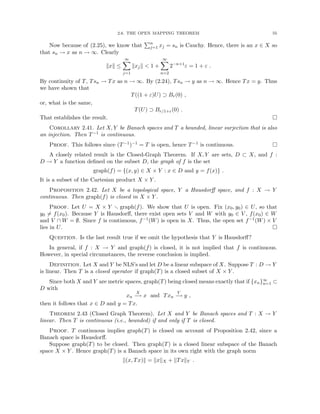
100. 100 4. SPECTRAL THEORY AND COMPACT OPERATORS
Proof. (a) We compute
(Tx, x) = (x, Tx) = (x, T∗x) = (Tx, x) ∈ R .
(b) By (a), we need only show the converse. This will follow if we can show that
(Tx, y) = (T∗
x, y) ∀ x, y ∈ H .
Let α ∈ C and compute
R 3
T(x + αy), x + αy
= (Tx, x) + |α|2
(Ty, y) + α(Ty, x) + ᾱ(Tx, y) .
The first two terms on the right are real, so also the sum of the latter two. Thus
R 3 ᾱ(Tx, y) + ᾱ(T∗x, y) .
If α = 1, we conclude that the complex parts of (Tx, y) and (T∗x, y) agree; if α = i, the real
parts agree.
We isolate an important result that is useful in other contexts.
Lemma 4.21. Suppose X and Y are Banach spaces and T ∈ B(X, Y ). Suppose that T is
bounded below, i.e., there is some γ 0 such that
kTxkY ≥ γkxkX ∀ x ∈ X .
Then T is one-to-one and R(T) is closed in Y .
Proof. That T is one-to-one is clear by linearity. Suppose for n = 1, 2, . . . , yn = Txn is a
sequence in R(T) and that yn → y ∈ Y . Then {yn}∞
n=1 is Cauchy, so also is {xn}∞
n=1. Since X is
complete, there is x ∈ X such that xn → x. Since T is continuous, yn = Txn → Tx = y ∈ R(T);
that is, R(T) is closed.
Theorem 4.22. Let H be a Hilbert space and T ∈ B(H, H) be a self-adjoint operator. Then
σr(T) = ∅ and
σ(T) ⊂ [r, R] ⊂ R ,
where
r = inf
kxk=1
(Tx, x) and R = sup
kxk=1
(Tx, x) .
Moreover, λ ∈ ρ(T) if and only if Tλ is bounded below.
Proof. If λ ∈ σp(T) and Tx = λx for x 6= 0, then λ(x, x) = (Tx, x) = (x, Tx) = (x, λx) =
λ̄(x, x); thus λ = λ̄ is real. If λ ∈ ρ(T), then the final conclusion follows from the boundedness
of T−1
λ ,
kxk = kT−1
λ Tλxk ≤ kT−1
λ k kTλxk ,
and the fact that T−1
λ 6≡ 0. Conversely, suppose Tλ is bounded below. By Lemma 4.21, Tλ is
one-to-one and R(Tλ) is closed. If R(Tλ) 6= H, then there is some x0 ∈ R(Tλ)⊥, and, ∀ x ∈ H,
0 = (Tλx, x0) = (Tx, x0) − λ(x, x0)
= (x, Tx0) − λ(x, x0)
= (x, Tλ̄x0) .

101. 4.4. BOUNDED SELF-ADJOINT LINEAR OPERATORS ON A HILBERT SPACE 101
Thus Tλ̄x0 = 0, or Tx0 = λ̄x0 and λ̄ ∈ σp(T). But then λ = λ̄ ∈ σp(T), and Tλ is not one-to-one,
a contradiction. Thus R(Tλ) = H and λ ∈ ρ(T).
Suppose now λ = α + iβ ∈ σ(T), where α, β ∈ R. For any x 6= 0 in H,
(Tλx, x) = (Tx, x) − λ(x, x)
and
(Tλx, x) = (Tx, x) − λ̄(x, x) ,
since (Tx, x) is real. Thus
(Tλx, x) − (Tλx, x) = −2iβ(x, x) ,
or
|β| kxk2
=
1
2
(Tλx, x) − (Tλx, x) ≤ kTλxk kxk .
As x 6= 0, we see that if β 6= 0, Tλ is bounded below, and conclude λ ∈ ρ(T), a contradiction.
Thus σ(T) ⊂ R.
Now suppose that σr(T) is not empty. Let λ ∈ σr(T). Then Tλ is invertible on its range
T−1
λ : R(Tλ) → H ,
but
R(Tλ) 6= H .
Let
y ∈ R(Tλ)
⊥
{0} .
Then, ∀ x ∈ H,
0 = (Tλx, y) = (x, Tλy) .
Let x = Tλy to conclude that Tλy = 0, i.e., λ ∈ σp(T). Since σr(T) ∩ σp(T) = ∅, we have our
contradiction, and conclude that σr(T) = ∅.
Finally, we bound the spectrum. Let c 0 and let λ = R + c R. Let x 6= 0 and compute
(Tx, x) = kxk2
T
x
kxk
,
x
kxk
≤ kxk2
R .
On the other hand,
−(Tx − λx, x) = −(Tλx, x) ≤ kTλxk kxk ,
and
−(Tx − λx, x) = −(Tx, x) + λkxk2
≥ −kxk2
R + λkxk2
= ckxk2
.
It is concluded that
kTλxk ≥ ckxk ;
hence, λ ∈ ρ(T).
A similar argument applies in case λ = r − c where c 0. Write for x 6= 0
(Tx, x) = kxk2
T
x
kxk
,
x
kxk
≥ kxk2
r .

102. 102 4. SPECTRAL THEORY AND COMPACT OPERATORS
On the other hand,
(Tx − λx, x) = (Tλx, x) ≤ kTλxk kxk ,
and
(Tx − λx, x) = (Tx, x) − λkxk2
≥ (r − λ)kxk2
= ckxk2
,
so λ ∈ ρ(T).
We call
q(x) =
(Tx, x)
(x, x)
∀ x 6= 0
the Rayleigh quotient of T at x. The result above is that
σ(T) ⊂
inf
x6=0
q(x) , sup
x6=0
q(x)
.
The next result shows the importance of the Rayleigh quotient of a self-adjoint operator.
Theorem 4.23. Let H be a Hilbert space and T ∈ B(H, H) self-adjoint. Then
r = inf
kxk=1
(Tx, x) ∈ σ(T) and R = sup
kxk=1
(Tx, x) ∈ σ(T) .
Moreover,
kTkB(X,X) = sup
kxk=1
|(Tx, x)| = max(|r|, |R|) .
That is, the minimal real number in σ(T) is r, and the maximal number in σ(T) is R, the
infimal and supremal values of the Rayleigh quotient. Moreover, kTk = max(|r|, |R|).
Proof. Let
M = sup
kxk=1
|(Tx, x)| .
Obviously,
M ≤ kTk .
If T ≡ 0, we are done, so let z ∈ H be such that Tz 6= 0 and kzk = 1. Set
v = kTzk1/2
z , w = kTzk−1/2
Tz .
Then
kvk2
= kwk2
= kTzk
and, since T is self-adjoint
T(v + w), v + w
−
T(v − w), v − w
= 2
h
(Tv, w) + (Tw, v)
i
= 4kTzk2
,
and
T(v + w), v + w
−
T(v − w), v − w
≤
T(v + w), v + w
+
T(v − w), v − w
≤ M kv + wk2
+ kv − wk2
= 2M kvk2
+ kwk2
= 4MkTzk .

103. 4.4. BOUNDED SELF-ADJOINT LINEAR OPERATORS ON A HILBERT SPACE 103
We conclude that
kTzk ≤ M ,
and, taking the supremum over all such z,
kTk ≤ M .
Thus kTk = M.
Obviously, λ ∈ σ(T) if and only if λ + µ ∈ σ(Tµ), so by such a translation, we may assume
that 0 ≤ r ≤ R. Then kTk = R and there is a sequence {xn}∞
n=1 such that kxnk = 1 and
(Txn, xn) = R −
1
n
.
Now
kTRxnk2
= kTxn − Rxnk2
= kTxnk2
− 2R(Txn, xn) + R2
≤ 2R2
− 2R
R −
1
n
=
2R
n
→ 0 .
Thus TR is not bounded below, so R /
∈ ρ(T), i.e., R ∈ σ(T). Similar arguments show r ∈
σ(T).
We know that if T ∈ B(H, H) is self-adjoint, then (Tx, x) ∈ R for all x ∈ H.
Definition. If H is a Hilbert space and T ∈ B(H, H) satisfies
(Tx, x) ≥ 0 ∀ x ∈ H ,
then T is said to be a positive operator. We denote this fact by writing 0 ≤ T. Moreover, if
R, S ∈ B(H, H), then R ≤ S means that 0 ≤ S − R.
Proposition 4.24. Suppose H is a complex Hilbert space and T ∈ B(H, H). Then T is a
positive operator if and only if σ(T) ≥ 0. Moreover, if T is positive, then T is self-adjoint.
Proof. This follows from Proposition 4.20 and Theorem 4.22.
An interesting and useful fact about a positive operator is that it has a square root.
Definition. Let H be a Hilbert space and T ∈ B(H, H) be positive. An operator S ∈
B(H, H) is said to be a square root of T if
S2
= T .
If, in addition, S is positive, then S is called a positive square root of T, denoted by
S = T1/2
.
Theorem 4.25. Every positive operator T ∈ B(H, H), where H is a Hilbert space, has a
unique positive square root.
The proof is long but not difficult. We omit it and refer the interested reader to [Kr,
p. 473–479].

104. 104 4. SPECTRAL THEORY AND COMPACT OPERATORS
Examples. (a) Let H = L2(Ω) for some Ω ⊂ Rd and φ : Ω → R a positive and bounded
function. Then T : H → H defined by
(Tf)(x) = φ(x)f(x) ∀ x ∈ Ω
is a positive operator, with positive square root
(Sf)(x) =
p
φ(x) f(x) ∀ x ∈ Ω .
(b) If T ∈ B(H, H) is any operator, then T∗T is positive.
4.5. Compact Self-Adjoint Operators on a Hilbert Space
On a Hilbert space, we can be very specific about the structure of a self-adjoint, compact
operator. In this case, the spectrum is real, countable, and nonzero values are eigenvalues with
finite dimensional eigenspaces. Moreover, if the number of eigenvalues is infinite, then they
converge to 0.
Theorem 4.26 (Hilbert-Schmidt). Let H be a Hilbert space, T ∈ C(H, H), and T = T∗.
There is an ON set {un} of eigenvectors corresponding to non-zero eigenvalues {λn} of T such
that every x ∈ H has a unique decomposition of the form
x =
X
αnun + v ,
where αn ∈ C and v ∈ N(T).
Proof. By Theorem 4.23, there is an eigenvalue λ1 of T such that
|λ1| = sup
kxk=1
|(Tx, x)| .
Let u1 be an associated eigenvector, normalized so that ku1k = 1. Let Q1 = {u1}⊥. Then Q1 is
a closed linear subspace of H, so Q1 is a Hilbert space in its own right. Moreover, if x ∈ Q1, we
have by self-adjointness that
(Tx, u1) = (x, Tu1) = λ1(x, u1) = 0 ,
so Tx ∈ Q1. Thus T : Q1 → Q1 and we may conclude by Theorem 4.23 that there is an
eigenvalue λ2 with
|λ2| = sup
kxk=1
x∈Q1
|(Tx, x)| .
Let u2 be a normalized eigenvector corresponding to λ2. Plainly, u1 ⊥ u2. Let
Q2 = {x ∈ Q1 : x ⊥ u2} = {u1, u2}⊥
.
Arguing inductively, there obtains a sequence of closed linear subspaces {Qn}. At the n-th stage,
we note that if x ∈ Qn = {u1, . . . , un}⊥, then for j = 1, . . . , n,
(Tx, uj) = (x, Tuj) = λj(x, uj) = 0 ,
so T : Qn → Qn. Thus there is an eigenvalue λn+1 with
|λn+1| = sup
kxk=1
x∈Qn
|(Tx, x)|
and an eigenvector un+1 with kun+1k = 1 corresponding to λn+1.

105. 4.5. COMPACT SELF-ADJOINT OPERATORS ON A HILBERT SPACE 105
Two possibilities occur. Either we reach a point where |(Tx, x)| 0 for some x ∈ Qn but
(Tx, x) = 0 (4.5)
for all x ∈ Qn+1 for some n, or we do not. If (4.5) is obtained, then with T1 = T|Qn+1 , our
theory shows that
kT1k = sup
kxk=1
x∈Qn+1
|(Tx, x)| = 0 .
Hence T vanishes on Qn+1, and Qn+1 ⊂ N(T). Equality must hold since T does not vanish
on span{u1, . . . , un} {0}, as Tx =
Pn
j=1 λjαjuj = 0 only if each αj = 0 (the λj 6= 0). Thus
Qn+1 = N(T) and we have the orthogonal decomposition from H = span{u1, . . . , un} ⊕ Qn+1:
Every x ∈ H may be written uniquely as
x =
n
X
j=1
αjuj + v
for some v ∈ {u1, . . . , un}⊥ = Qn+1.
If the procedure does not terminate in a finite number of steps, it generates an infinite
sequence of eigenvalues {λn}∞
n=1 and eigenvectors {un}∞
n=1. By our general results, we know
that although the λn may repeat, each can do so only a finite number of times. Thus
λn → 0 as n → ∞ .
Let H1 be the Hilbert space generated by the ON family {un}∞
n=1. Every element x ∈ H is
written uniquely in the form
x =
∞
X
j=1
(x, uj)uj + v
for some v ∈ H⊥
1 , since H = H1 ⊕ H⊥
1 . It remains to check that H⊥
1 = N(T). Let v ∈ H⊥
1 ,
v 6= 0. Now,
H⊥
1 ⊂ Qn for all n = 1, 2, . . . ,
so it must obtain that
|(Tv, v)|
kvk2
≤ sup
x∈Qn
|(Tx, x)|
kxk2
= |λn+1| .
The right-hand side tends to zero as n → +∞, whereas the left-hand side does not depend on
n. It follows that
(Tv, v) = 0 for all v ∈ H⊥
1 .
Thus T2 = T|H⊥
1
vanishes, as
kT2k = sup
kvk=1
v∈H⊥
1
|(Tv, v)| = 0 ,
so H⊥
1 ⊂ N(T). For x ∈ H1, for some scalars βn,
Tx = T
∞
X
n=1
βnun
!
=
∞
X
n=1
βnTun =
∞
X
n=1
λnβnun ∈ H1,

106. 106 4. SPECTRAL THEORY AND COMPACT OPERATORS
and we conclude that T : H1 → H1 is one-to-one and onto (each λn 6= 0). Thus N(T)∩H1 = {0},
so N(T) = H⊥
1 .
Theorem 4.27 (Spectral Theorem for Self-Adjoint Compact Operators). Let T ∈ C(H, H)
be a self-adjoint operator on a Hilbert space H. Then there exists an ON base {vα}α∈I for H
such that each vα is an eigenvector for T. Moreover, for every x ∈ H,
Tx =
X
α∈I
λα(x, vα)vα , (4.6)
where λα is the eigenvalue corresponding to vα.
Proof. Let {un} be the ON system constructed in the last theorem. Let H1 be the closed
subspace spann{un}. Let {eβ}β∈J be an ON base for H⊥
1 . Then
{eβ}β∈J ∪ {un}
is an ON base for H. Moreover,
Teβ = 0 ∀ β ∈ J ,
so the eβ are eigenvalues corresponding to the eigenvalue 0.
We know that for x ∈ H, there is v ∈ N(T) such that
N
X
n=1
(x, un)un + v
converges to x in H. Because T is continuous,
N
X
n=1
λn(x, un)un = T
N
X
n=1
(x, un)un + v
→ Tx .
That is, (4.6) holds since λα = 0 for any index α corresponding to an eβ, β ∈ J .
We have represented a self-adjoint T ∈ C(H, H) as an infinite, diagonal matrix of its eigen-
values. It should come as no surprise that if T is a positive operator, S defined by
Sx =
X
α∈I
p
λα (x, uα)uα
is the positive square root of T. We leave it to the reader to verify this statement, as well as the
implied fact that S ∈ C(H, H).
Proposition 4.28. Let S, T ∈ C(H, H) be self-adjoint operators on a Hilbert space H.
Suppose ST = TS. Then there exists an ON base {vα}α∈I for H of common eigenvectors of S
and T.
Proof. Let λ ∈ σ(S) and let Vλ be the corresponding eigenspace. For any x ∈ Vλ,
STx = TSx = T(λx) = λTx ⇒ Tx ∈ Vλ .
Therefore T : Vλ → Vλ. Now T is self-adjoint on Vλ and compact, so it has a complete ON set
of T-eigenvectors. This ON set are also eigenvectors for S since everything in Vλ is such.

107. 4.6. THE ASCOLI-ARZELÀ THEOREM 107
4.6. The Ascoli-Arzelà Theorem
We now discuss important examples of compact operators called integral operators. These
are operators of the form
(Tf)(x) =
Z
Ω
K(x, y)f(y) dy ,
where f is in an appropriate Hilbert (or Banach) space and K satisfies appropriate hypothesis.
To demonstrate compactness, we will derive a more general result, known as the Ascoli-Arzelà
Theorem, about compact metric spaces.
Lemma 4.29. A compact metric space (M, d) is separable (i.e., it has a countable dense
subset).
Proof. For any integer n ≥ 1, cover M by balls of radius 1/n:
M =
[
x∈M
B1/n(x) .
By compactness, we can extract a finite subcover
M =
Nn
[
i=1
B1/n(xn
i ) (4.7)
for some xn
i ∈ M. The set
S = {xn
i | i = 1, . . . , Nn ; n = 1, 2 . . . }
is countable, and we claim that it is dense in M. Let x ∈ M and ε 0 be given. For n large
enough that 1/n ≤ ε, by (4.7), there is some xn
j ∈ S such that
x ∈ B1/n(xn
j ) ;
that is, d(x, xn
j ) 1/n ≤ ε. Thus indeed S is dense.
Theorem 4.30 (Ascoli-Arzelà). Let (M, d) be a compact metric space and let
C(M) = C(M; F)
denote the Banach space of continuous functions from M to F with the maximum norm
kfk = max
x∈M
|f(x)| .
Let A ⊂ C(M) be a subset that is bounded and equicontinuous, which is to say, respectively, that
for some R 0,
kfk ≤ R ∀f ∈ A ,
(i.e., A ⊂ BR(0)), and, given ε 0 there is δ 0 such that
max
d(x,y)δ
|f(x) − f(y)| ε ∀f ∈ A . (4.8)
Then the closure of A, Ā, is compact in C(M).

108. 108 4. SPECTRAL THEORY AND COMPACT OPERATORS
Proof. It suffices by Lemma 4.9 to show that an arbitrary sequence {fn}∞
n=1 ⊂ A has a
convergent subsequence. For each fixed x ∈ M, {fn(x)}∞
n=1 is bounded in F by R, and so it has
a convergent subsequence. Let {xj}∞
j=1 be a countable dense subset of M. By a diagonalization
argument, we can extract a single subsequence {fnk
}∞
k=1 such that {fnk
(xj)}∞
k=1 converges for
each j. The argument is as follows. Let {fnk(x1)(x1)}∞
k=1 be convergent, and from the bounded
set {fnk(x1)(x2)}∞
k=1, select a convergent subsequence {fnk(x2)(x2)}∞
k=1. Continuing, we obtain
indices
{nk(x1)}∞
k=1 ⊃ {nk(x2)}∞
k=1 ⊃ · · ·
such that {fnk(xi)(xj)}∞
k=1 converges for all j ≤ i. Finally, {fnk(xk)}∞
k=1 is our desired subse-
quence.
Now let ε 0 be given and fix x ∈ M. Let δ 0 correspond to ε via (4.8). There exists a
finite subset {x̃m}N
m=1 ⊂ {xj}∞
j=1 such that
N
[
m=1
Bδ(x̃m) ⊃ M ,
since M is compact. Choose x̃` such that
d(x, x̃`) δ .
Then for any i, j, by (4.8),
|fni (x) − fnj (x)|
≤ |fni (x) − fni (x̃`)| + |fni (x̃`) − fnj (x̃`)| + |fnj (x̃`) − fnj (x)|
≤ 2ε + |fni (x̃`) − fnj (x̃`)|
≤ 2ε + max
1≤m≤N
|fni (x̃m) − fnj (x̃m)| .
(4.9)
Since each sequence of real numbers {fnk
(x̃m)}∞
k=1 is Cauchy, we conclude that {fnk
(x)}∞
k=1 is
also Cauchy. Now define f : M → F by
f(x) = lim
k→∞
fnk
(x) .
This is the pointwise limit. However, since the right-hand side of (4.9) is independent of x,
we conclude that in fact the convergence is uniform, i.e., the convergence is in the norm of
C(M).
Theorem 4.31. Let Ω ⊂ Rd be bounded and open, and K continuous on Ω × Ω. Let
X = C( Ω ) and define T : X → X by
Tf(x) =
Z
Ω
K(x, y)f(y) dy
(that T is well defined is easily checked). Then T is compact.
Proof. Let {fn}∞
n=1 be bounded in M. We must show that {Tfn}∞
n=1 has a convergent
subsequence. Since Ω is a compact metric space, the Ascoli-Arzelà theorem implies the result if
the image of our sequence is bounded and equicontinuous. The former follows since
kTfnkL∞(Ω) ≤ kfnkL∞(Ω)kKkL∞(Ω×Ω)
Z
Ω
dx

109. 4.7. STURM LIOUVILLE THEORY 109
is bounded independently of n. For equicontinuity, we compute
|Tfn(x) − Tfn(y)| =
Z
Ω
(K(x, z) − K(y, z))fn(z) dz
≤ kfnkL∞ sup
z∈Ω
|K(x, z) − K(y, z)|
Z
Ω
dx .
Since K is uniformly continuous on Ω × Ω, the right-side above can be made uniformly small
provided |x − y| is taken small enough.
By an argument based on the density of C( Ω ) in L2(Ω), and the fact that the limit of
compact operators is compact, we can extend this result to L2(Ω). The details are left to the
reader.
Corollary 4.32. Let Ω ⊂ Rd be bounded and open. Suppose K ∈ L2(Ω × Ω) and
T : L2(Ω) → L2(Ω) is defined as in the previous theorem. Then T is compact.
4.7. Sturm Liouville Theory
Suppose I = [a, b] ⊂ R, aj ∈ C2−j(I), j = 0, 1, 2 and a0 0. We consider the operator
L : C2(I) → C(I) defined by
(Lx)(t) = a0(t)x00
(t) + a1(t)x0
(t) + a2(t)x(t) .
Note that L is a bounded linear operator.
Theorem 4.33 (Picard). Given f ∈ C(I) and x0, x1 ∈ R, there exists a unique solution
x ∈ C2(I) to the initial value problem (IVP)
(
Lx = f ,
x(a) = x0 , x0(a) = x1 .
(4.10)
Consult a text on ordinary differential equations for a proof.
Corollary 4.34. The null space N(L) is two dimensional.
Proof. We construct a basis. Solve (4.10) with f = x1 = 0, x0 = 1. Call this solution
z0(t). Clearly z0 ∈ N(L). Now solve for z1(t) with f = x0 = 0, x1 = 1. Then any x ∈ N(L)
solves (4.10) with x0 = x(a) and x1 = x0(a), so
x(t) = x(a)z0(t) + x0
(a)z1(t) ,
by uniqueness.
Thus, to solve (4.10), we cannot find L−1 (it does not exist). Rather, the inverse operator
we desire concerns both L and the initial conditions. Ignoring these conditions for a moment,
we study the structure of L within the context of an inner-product space.
Definition. The formal adjoint of L is denoted L∗ and defined by L∗ : C2(I) → C(I)
where
(L∗
x)(t) = (ā0x)00
− (ā1x)0
+ ā2x
= ā0x00
+ (2ā0
0 − ā1)x0
+ (ā00
0 − ā0
1 + ā2)x .

110. 110 4. SPECTRAL THEORY AND COMPACT OPERATORS
The motivation is the L2(I) inner-product. If x, y ∈ C2(I), then
(Lx, y) =
Z b
a
Lx(t)ȳ(t) dt
=
Z b
a
[a0x00
ȳ + a1x0
ȳ + a2xȳ ] dt
=
Z b
a
xL∗y dt + [a0x0
ȳ − x(a0ȳ )0
+ a1xȳ ]b
a
= (x, L∗
y) + Boundary terms.
Definition. If L = L∗, we say that L is formally self-adjoint. If a0, a1, and a2 are real-
valued functions, we say that L is real.
Proposition 4.35. The real operator L = a0D2 + a1D + a2 is formally self-adjoint if and
only if a0
0 = a1. In this case,
Lx = (a0x0
)0
+ a2x = D(a0D)x + a2x ,
i.e.,
L = Da0D + a2 .
Proof. Note that for a real operator,
L∗
= a0D2
+ (2a0
0 − a1)D + (a00
0 − a0
1 + a2) ,
so L = L∗ if and only if
a1 = 2a0
0 − a1 ,
a2 = a00
0 − a0
1 + a2 .
That is,
a1 = a0
0 and a0
1 = a00
0 ,
or simply the former condition. Then
Lx = a0D2
x + a0
0Dx + a2x = D(a0Dx) + a2x .
Remark. If L = a0D2 + a1D + a2 is real but not formally self-adjoint, we can render it so
by a small adjustment using the integrating factor
Q(t) =
1
a0(t)
P(t) ,
P(t) = exp
Z t
a
a1(τ)
a0(τ)
dτ
0 ,
for which P0 = a1P/a0. Then
Lx = f ⇐⇒ L̃x = ˜
f ,
where
L̃ = QL and ˜
f = Qf .

111. 4.7. STURM LIOUVILLE THEORY 111
But L̃ is formally self-adjoint, since
L̃x = QLx = Px00
+
a1
a0
Px0
+ a2Qx
= Px00
+ P0
x0
+ a2Qx
= (Px0
) +
a2
a0
P
x .
Examples. The most important examples are posed for I = (a, b), a or b possibly infinite,
and aj ∈ C2−j( ¯
I ), where a0 0 on I (thus a0(a) and a0(b) may vanish — we have excluded
this case, but the theory is similar).
(a) Legendre:
Lx = ((1 − t2
)x0
)0
, −1 ≤ t ≤ 1 .
(b) Chebyshev:
Lx = (1 − t2
)1/2
((1 − t2
)1/2
x0
)0
, −1 ≤ t ≤ 1 .
(c) Laguerre:
Lx = et
(te−t
x0
)0
, 0 t ∞ .
(d) Bessel: for ν ∈ R,
Lx =
1
t
(tx0
)0
−
ν2
t2
x , 0 t 1 .
(e) Hermite:
Lx = et2
(e−t2
x0
)0
, t ∈ R .
We now include and generalize the initial conditions, which characterize N(L). Instead of
two conditions at t = a, we consider one condition at each end of I = [a, b], called boundary
conditions (BC’s).
Definition. Let p, q, and w be real-valued functions on I = [a, b], a b both finite, with
p 6= 0 and w 0. Let α1, α2, β1, and β2 ∈ R be such that
α2
1 + α2
2 6= 0 and β2
1 + β2
2 6= 0 .
Then the problem of finding x(t) ∈ C2(I) and λ ∈ C such that





Ax ≡ 1
w [(px0)0 + qx] = λx , t ∈ (a, b) ,
α1x(a) + α2x0(a) = 0 ,
β1x(b) + β2x0(b) = 0 ,
(4.11)
is called a regular Sturm-Liouville (regular SL) problem. It is the eigenvalue problem for A with
the BC’s.
We remark that if a or b are infinite or p vanishes at a or b, the corresponding BC is lost
and the problem is called a singular Sturm-Liouville problem.
Example. Let I = [0, 1] and
(
Ax = −x00 = λx , t ∈ (0, 1) ,
x(0) = x(1) = 0 .
(4.12)

112. 112 4. SPECTRAL THEORY AND COMPACT OPERATORS
Then we need to solve
x00
+ λx = 0 ,
which as we saw has the 2 dimensional form
x(t) = A sin
√
λ t + b cos
√
λ t
for some constants A and B. Now the BC’s imply that
x(0) = B = 0 ,
x(1) = A sin
√
λ = 0 .
Thus either A = 0 or, for some integer n,
√
λ = nπ ;
that is, non trivial solutions are given only for the eigenvalues
λn = n2
π2
,
and the corresponding eigenfunctions are
xn(t) = sin(nπt)
(or any nonzero multiple).
To analyze a regular SL problem, it is helpful to notice that
A : C2
(I) → C0
(I)
has strictly larger range. However, its inverse (with the BC’s), would map C0(I) to C2(I) ⊂
C0(I). So the inverse might be a bounded linear operator with known spectral properties,
which can then be related to A itself. This is the case, and leads us to the classical notion of
a Green’s function. The Green’s function allows us to construct the solution to the boundary
value problem





Ax = f , t ∈ (a, b) ,
α1x(a) + α2x0(a) = 0 ,
β1x(b) + β2x0(b) = 0 ,
(4.13)
for any f ∈ C0(I).
Definition. A Green’s function for the regular SL problem (4.11) is a function G : I×I → R
such that
(a) G ∈ C0(I × I) and G ∈ C2(I × I D), where D = {(t, t) : t ∈ I} is the diagonal in
I × I;
(b) For each fixed s ∈ I, G(·, s) satisfies the BC’s of the problem;
(c) A applied to the first variable t of G(t, s), also denoted AtG(t, s), vanishes for (t, s) ∈
I × I D, i.e.,
AtG(t, s) ≡
1
w
∂
∂t
p(t)
∂G
∂t
(t, s)
+ q(t)G(t, s)
= 0 ∀ t 6= s ;
(d) lim
s→t−
∂G
∂t
(t, s) − lim
s→t+
∂G
∂t
(t, s) =
1
p(t)
for all t ∈ (a, b).

113. 4.7. STURM LIOUVILLE THEORY 113
Example. Corresponding to (4.12), consider
(
Ax = −x00 = f , t ∈ (0, 1) ,
x(0) = x(1) = 0 ,
(4.14)
for f ∈ C0(I). Let
G(t, s) =
(
(1 − t)s , 0 ≤ s ≤ t ≤ 1 ,
(1 − s)t , 0 ≤ t ≤ s ≤ 1 .
Then G satisfies (a) and
G(0, s) = (1 − s) · 0 = 0 ,
G(1, s) = (1 − (1))s = 0 ,
so (b) holds. Since w = 1, p = −1, and q = 0,
AtG(t, s) = −
∂2
∂t2
G(t, s) = 0 for s 6= t
and
lim
s→t−
∂G
∂t
= −t , lim
s→t+
∂G
∂t
= 1 − t ,
we also have (c) and (d). Thus G(t, s) is our Green’s function. Moreover, if we define
x(t) =
Z 1
0
G(t, s)f(s) ds ,
then x(0) = x(1) = 0 and
x0
(t) =
d
dt
Z t
0
G(t, s)f(s) ds +
Z 1
t
G(t, s)f(s) ds
= G(t, t)f(t) +
Z t
0
∂G
∂t
(t, s)f(s) ds − G(t, t)f(t) +
Z 1
t
∂G
∂t
(t, s)f(s) ds
=
Z 1
0
∂G
∂t
(t, s)f(s) ds ,
x00
(t) =
d
dt
Z t
0
∂G
∂t
f ds +
Z 1
t
∂G
∂t
f ds
=
∂G
∂t
(t, t−
)f(t) +
Z t
0
∂2G
∂t2
f ds −
∂G
∂t
(t, t+
)f(t) +
Z 1
t
∂2G
∂t2
f ds
= −f +
Z 1
0
∂2G
∂t2
f ds
= −f(t) .
Thus we constructed a solution to (4.14) with G(t, s).

114. 114 4. SPECTRAL THEORY AND COMPACT OPERATORS
Theorem 4.36. Suppose that for the regular SL system (so α2
1 + α2
2 0 and β2
1 + β2
2 0)







Au ≡
1
w
Lu ≡
1
w
[(pu0
)0
+ qu] = f , t ∈ (a, b) ,
α1u(a) + α2u0(a) = 0 ,
β1u(b) + β2u0(b) = 0 ,
on the interval I = [a, b], p ∈ C1(I), w, q ∈ C0(I), and p, w 0. Suppose also that 0 is not
an eigenvalue (so Au = 0 with the BC’s implies u = 0). Let u1 and u2 be any nonzero real
solutions of Au = Lu = 0 such that for u1,
α1u1(a) + α2u0
1(a) = 0 ,
and for u2,
β1u2(b) + β2u0
2(b) = 0 .
Define G : I × I → R by
G(t, s) =







u2(t)u1(s)
pW
, a ≤ s ≤ t ≤ b ,
u1(t)u2(s)
pW
, a ≤ t ≤ s ≤ b ,
where p(t) W(t) is a nonzero constant and
W(s) = W(s; u1, u2) ≡ u1(s)u0
2(s) − u0
1(s)u2(s)
is the Wronskian of u1 and u2. Then G is a Green’s function for L. Moreover, if G is any
Green’s function for L and f ∈ C0(I), then
u(t) =
Z b
a
G(t, s)f(s) ds (4.15)
is the unique solution of Lu = f satisfying the BC’s.
To solve Au = f, just solve Lu = wf:
u(t) =
Z b
a
G(t, s)f(s)w(s) ds .
We first prove two lemmas concerning the Wronskian.
Lemma 4.37 (Abel). Let Lu = (pu0)0 +qu satisfy p ∈ C1(I) and q ∈ C0(I). For any positive
w ∈ C0(I) and λ ∈ C, if u1 and u2 solve
Lu = λwu ,
then
p(t)W(t; u1, u2)
is constant.

115. 4.7. STURM LIOUVILLE THEORY 115
Proof. We compute
0 = λw(u1u2 − u2u1)
= u1Lu2 − u2Lu1
= u1(pu00
2 + p0
u0
2 + qu2) − u2(pu00
1 + p0
u0
1 + qu1)
= p(u1u00
2 − u2u00
1) + p0
W
= (pW)0
.
Lemma 4.38. Suppose u, v ∈ C1(I). If W(t0; u, v) 6= 0 for some t0 ∈ I, then u and v are
linearly independent. If u and v are linearly independent, then W(t; u, v) 6= 0 for all t ∈ I.
Proof. Suppose for some scalars α and β,
αu(t) + βv(t) = 0 ,
so also
αu0
(t) + βv0
(t) = 0 .
At t = t0, we have a linear system
u(t0) v(t0)
u0(t0) v0(t0)
α
β
=
0
0
,
which is uniquely solvable if the matrix is invertible, i.e., if its determinant, W(t0) 6= 0. Thus
α = β = 0 and we conclude that u and v are linearly independent.
Conversely, the linear independence of u and v requires the determinant W(t) 6= 0 for each
t ∈ I.
Proof of Theorem 4.36. The existence of u1 and u2 follows from Picard’s Theorem 4.33.
If we use the standard basis
N(L) = span{z0, z1} ,
where
z0(a) = 1 , z0
0(a) = 0 ,
z1(a) = 0 , z0
1(a) = 1 ,
then
u1(t) = −α2z0(t) + α1z1(t) 6≡ 0 .
A similar construction at t = b gives u2(t).
If u1 = λu2 for some λ ∈ C, i.e., u1 and u2 are linearly dependent, then u1 6≡ 0 satisfies both
boundary conditions, since λ cannot vanish, and the equation Lu1 = 0, contrary to the hypoth-
esis that 0 is not an eigenvalue to the SL problem. Thus u1 and u2 are linearly independent,
and by our two lemmas pW is a nonzero constant. Thus G(t, s) is well defined.
Clearly G is continuous and C2 when t 6= s, since u1, u2 ∈ C2(I). Moreover, G(·, s) satisfies
the BC’s by construction, and AtG is either Au1 = 0 or Au2 = 0 for t 6= s. Thus it remains

116. 116 4. SPECTRAL THEORY AND COMPACT OPERATORS
only to show the jump condition on ∂G/∂t of the definition of a Green’s function. But
∂G
∂t
(t, s) =







u0
2(t)u1(s)
pW
, a ≤ s ≤ t ≤ b ,
u0
1(t)u2(s)
pW
, a ≤ t ≤ s ≤ b ,
so
∂G
∂t
(t, t−
) −
∂G
∂t
(t, t+
) =
u0
2(t)u1(t)
pW
−
u0
1(t)u2(t)
pW
=
1
p(t)
.
If Lu = f has a solution, it must be unique since the difference of two such solutions would
satisfy the eigenvalue problem with eigenvalue 0, and therefore vanish. Thus it remains only to
show that u(t) defined by (4.15) is a solution to Lu = f. We use only (a)–(d) in the definition
of a Green’s function.
Trivially u satisfies the two BC’s by (b) and the next computation. We compute for t ∈ (a, b)
using (a):
u0
(t) =
d
dt
Z b
a
G(t, s)f(s) ds
=
d
dt
Z t
a
G(t, s)f(s) ds
+
d
dt
Z b
t
G(t, s)f(s) ds
= G(t, t)f(t) +
Z t
a
∂G
∂t
(t, s)f(s) ds − G(t, t)f(t) +
Z b
t
∂G
∂t
(t, s)f(s) ds
=
Z b
a
∂G
∂t
(t, s)f(s) ds .
Then
(p(t)u0
(t))0
=
d
dt
Z t
a
p(t)
∂G
∂t
(t, s)f(s) ds
+
d
dt
Z b
t
p(t)
∂G
∂t
(t, s)f(s) ds
= p(t)
∂G
∂t
(t, t−
)f(t) +
Z t
0
∂
∂t
p(t)
∂G
∂t
(t, s)
f(s) ds
− p(t)
∂G
∂t
(t, t+
)f(t) +
Z b
t
∂
∂t
p(t)
∂G
∂t
(t, s)
f(s) ds
= f(t) +
Z b
a
∂
∂t
p(t)
∂G
∂t
(t, s)
f(s) ds ,
using (d). Finally, we use (c) to conclude
Lu(t) = (pu0
)0
+ qu
= f(t) +
Z b
a
AtG(t, s)f9s)w(t) ds
= f(t)
as required.
We define the solution operator
T : C0
(I) → C0
(I)

117. 4.7. STURM LIOUVILLE THEORY 117
by
Tf(t) =
Z b
a
G(t, s)f(s) ds ,
where G is our Green’s function. Endowing T with the L2(I) inner-product, we conclude that
T is a bounded linear operator, since for f ∈ C0(I),
kTfk2
≤
Z b
a
Z b
a
|G(t, s)| f(s)| ds
2
dt
≤
Z b
a
Z b
a
|G(t, s)|2
ds
Z b
a
|f(s)|2
ds dt
= kGkL
L2(I×I)kfk2
L2(I) .
Since G(s, t) = G(t, s) is real, we compute that for f, g ∈ C0(I),
(Tf, g) =
Z b
a
Z b
a
G(t, s)f(s) ds g(t) dt
=
Z b
a
f(s)
Z b
a
G(s, t) g(t) dt ds
= (f, Tg) ,
that is, T is self-adjoint. By the Ascoli-Arzelà theorem, we know that T is a compact operator.
The incompleteness of C0(I) is easily rectified, since C0(I) is dense in L2(I). We extend T
to L2(I) as follows. Given f ∈ L2(I), find fn ∈ C0(I) such that fn → f in L2(I). Then
boundedness implies that {Tfn}∞
n=1 is Cauchy in L2(I). So define
Tf = lim
n→∞
Tfn .
Then
T : L2(I) → L2(I)
is a continuous linear operator. Moreover, it is not difficult to conclude that the extended T
remains compact and self-adjoint.
We know much about the spectral properties of T. We relate these properties to those of
L = wA.
Proposition 4.39. If λ = 0 is not an eigenvalue of the regular SL problem, then λ = 0 is
not an eigenvalue of T either.
Proof. Suppose Tf = 0 for some f ∈ L2(I). Then, with c = (pW)−1,
0 = (Tf)0
(t) =
d
dt
cu2(t)
Z t
a
f(s)u1(s) ds + cu1(t)
Z b
t
f(s)u2(s) ds
= c
u0
2
Z t
a
fu1 ds + u0
1
Z b
t
fu2 ds
.
But
0 = Tf(t) = c
u2
Z t
a
fu1 ds + u1
Z b
t
fu2 ds
,

118. 118 4. SPECTRAL THEORY AND COMPACT OPERATORS
so, since W(t; u1, u2) 6= 0, the solution of this linear system is trivial; that is, for each t ∈ [a, b],
Z t
a
fu1 ds =
Z b
t
fu2 ds = 0 .
We conclude that
f(t)u1(t) = f(t)u2(t) = 0 ,
so f = 0, since u1 and u2 cannot both vanish at the same point (W 6= 0). Thus N(T) = {0}
and 0 /
∈ σp(T).
Proposition 4.40. Suppose λ 6= 0. Then λ is an eigenvalue of the regular SL problem if
and only if 1/λ is an eigenvalue of T. Moreover, the corresponding eigenspaces coincide.
Proof. If f ∈ C0(I) is an eigenfunction for L, then
Lf = λf ,
so
f = TLf = λTf
shows that
Tf =
1
λ
f .
Conversely, suppose f ∈ L2(I) is an eigenfunction for T:
Tf =
1
λ
f .
Since G is continuous, in fact R(T) ⊂ C0(I), so f ∈ C0(I) and
f = LTf =
1
λ
Lf .
We return to our original operator A = 1
w L. Define the inner-product on L2(I)
hf, giw =
Z b
a
f(t) g(t) w(t) dt .
This induces a norm equivalent to the usual L2(I)-norm, since
0 min
s∈I
w(s) ≤ w(t) ≤ max
s∈I
w(s) ∞
for all t ∈ I. Define K : L2(I) → L2(I) by
Kf(t) =
Z b
a
G(t, s)f(s)w(s) ds .
This is the solution operator for
Au = f .
With the usual inner-product on L2(I), K is not self-adjoint; however, with h·, ·iw, K is self-
adjoint. The proof of the following result is left as an exercise .

119. 4.7. STURM LIOUVILLE THEORY 119
Proposition 4.41. The operator K is self-adjoint and compact on (L2(I), h·, ·iw), 0 /
∈
σp(K), and
σ(K) = {0} ∪ {λ 6= 0 : 1/λ is an eigenvalue of A} .
Moreover, the eigenspaces of K and A coincide.
We know that dim(N(Tλ)) = dim(N(Kλ)) is finite. However, we can conclude directly that
eigenfunctions of a regular SL problem are simple (i.e., one dimensional).
Proposition 4.42. The eigenvalues of a regular SL problem are simple.
Proof. Suppose u and v are eigenvectors for λ 6= 0 an eigenvalue. Lemma 4.37 tells us
that pW = c for some constant c. If c = 0, then as p 6= 0, W ≡ 0 and u and v are linearly
independent. So suppose W(t0) 6= 0 for some t0. By Lemma 4.38, W 6= 0 for all t ∈ [a, b].
However, W(a) = 0 by the boundary conditions:
α1u(a) + α2u0
(a) = 0 ,
α1v(a) + α2v0
(a) = 0 ,
is a linear system with a nontrivial solution (α1, α2), so W(a), the determinant of the corre-
sponding matrix, vanishes. Thus u and v are linearly independent and λ is simple.
We summarize what we know about the regular SL problem for A based on the Spectral
Theorem for Compact Self-adjoint operators as applied to K. The details of the proof are left
as an exercise.
Theorem 4.43. Let a, b ∈ R, a b, I = [a, b], p ∈ C1(I), p 6= 0, q ∈ C0(I), and w ∈ C0(I),
w 0. Let
A =
1
w
[DpD + q]
be a formally self-adjoint regular SL operator with boundary conditions
α1u(a) + α2u0
(a) = 0 ,
β1u(b) + β2u0
(b) = 0 ,
for u ∈ C2(I), where α2
1 + α2
2 6= 0 and β2
1 + β2
2 6= 0, αi, βi ∈ R. If 0 is not an eigenvalue of A,
then A has a countable collection of real eigenvalues {λn}∞
n=1 such that
|λn| → ∞ as n → ∞
and each eigenspace is one-dimensional. Let {un}∞
n=1 be the corresponding normalized eigen-
functions. These form an ON basis for (L2(I), h·, ·iw), so if u ∈ L2(I),
u =
∞
X
n=1
hu, uniwun
and, provided Au ∈ L2(I),
Au =
∞
X
n=1
λnhu, uniwun .

120. 120 4. SPECTRAL THEORY AND COMPACT OPERATORS
We saw earlier that the regular SL problem
(
−x00 = λx , t ∈ (0, 1) ,
x(0) = x(1) = 0 ,
has eigenvalues
λn = n2
π2
, n = 1, 2, . . .
and corresponding (normalized) eigenfunctions
un(t) =
√
2 sin(nπt) .
Given any f ∈ L2(0, 1), we have its sine series
f(t) =
∞
X
n=1
2
Z 1
0
f(s) sin nπs ds
sin nπt ,
where equality holds for a.e. t ∈ [0, 1], i.e., in L2(0, 1). This shows that L2(0, 1) is separable.
By iterating our result, we can decompose any f ∈ L2(I × I), I = (0, 1). For a.e. x ∈ I,
f(x, y) =
∞
X
n=1
2
Z 1
0
f(x, t) sin nπt dt
sin nπy
= 4
∞
X
n=1
Z 1
0
∞
X
m=1
Z 1
0
f(s, t) sin mπs ds sin nπt dt sin nπy sin nπx
= 4
∞
X
n=1
∞
X
m=1
Z 1
0
Z 1
0
f(s, t) sin mπs sin nπt ds dt sin nπx sin nπy .
So L2(I × I) has the ON basis
{2 sin nπx sin nπy}∞,∞
m=1, n=1 ,
and again L2(I × I) is separable. Continuing, we can find a countable basis for any L2(R),
R = Id, d = 1, 2, . . . . By dilation and translation, we can replace R by any rectangle, and since
L2(Ω) ⊂ L2(R) whenever Ω ⊂ R (if we extend the domain of f ∈ L2(Ω) by defining f ≡ 0 on
R Ω), L2(Ω) is separable for any bounded Ω, but the construction of a basis is not so clear.
The regular SL problem
(
−x00 = λx , t ∈ (0, 1) ,
x0(0) = x0(1) = 0 ,
gives the eigenfunctions
un(t) =
√
2 cos(nπt) .
These are used to define cosine series expansions, similar to the development above. The
problem





−x00 = λx , t ∈ (0, 1) ,
x(0) = x(1) ,
x0(0) = x0(1) ,

121. 4.7. STURM LIOUVILLE THEORY 121
seeks a periodic solution. Although not a regular SL problem as defined above, a similar theory
produces a complete set of orthogonal eigenfunctions, which leads us to Fourier series:
un(t) =
√
2 cos(2nπt) and vn(t) =
√
2 sin(2nπt) .
Example. Let Ω = (0, a) × (0, b), and consider a solution u(x, y) of



−
∂2u
∂x2
−
∂2u
∂y2
= f(x, y) , (x, y) ∈ Ω ,
u(x, y) = 0 , (x, y) ∈ ∂Ω ,
where f ∈ L2(Ω). We proceed formally; that is, we compute without justifying our steps.
We justify the final result only. We use the technique called separation of variables. Suppose
v(x, y) = X(x)Y (y) is a solution to the eigenvalue problem
−X00
Y − XY 00
= λXY .
Then
−
X00
X
= λ +
Y 00
Y
= µ ,
a constant. Now the BC’s are
X(0) = X(a) = 0 ,
Y (0) = Y (b) = 0 ,
so X satisfies a SL problem with
µ = µm =
mπ
a
2
, m = 1, 2, . . . ,
Xm(x) = sin
mπx
a
.
Now, for each such m,
−Y 00
= (λm − µm)Y
has solution
λm,n − µm =
nπ
b
2
, n = 1, 2, . . . ,
Yn(y) = sin
nπy
b
.
That is, for m, n = 1, 2, . . . ,
λm,n =
m
a
2
+
n
b
2
π2
,
Vm,n(x, y) = sin
mπx
a
sin
nπy
b
.
We know that {vm,n} form a basis for L2((0, a) × (0, b)), so, rigorously, we expand
f(x, y) =
X
m,n
cm,nvm,n(x, y)
for the coefficients
cm,n =
R b
0
R a
0 f(x, y)vm,n(x, y) dx dy
R b
0
R a
0 v2
m,n(x, y) dx dy
.

122. 122 4. SPECTRAL THEORY AND COMPACT OPERATORS
Forming
u(x, y) ≡
X
m,n
cm,n
p
λm,n
vm,n(x, y) ,
we verify that indeed u is a solution to the problem.
4.8. Exercises
1. Let {xn}∞
n=1 be an orthonormal set in a Hilbert space H. Let {an}∞
n=1 be a sequence of
non-negative numbers and let
S =
x ∈ H : x =
∞
X
n=1
bnxn and |bn| ≤ an for all n
.
Show that S is compact if and only if
P∞
n=1 a2
n ∞.
2. Let H be a Hilbert space and P ∈ B(H, H) a projection.
(a) Show that P is an orthogonal projection if and only if P = P∗.
(b) If P is an orthogonal projection, find σp(P), σc(P), and σr(P).
3. Let A be a self-adjoint, compact operator on a Hilbert space. Prove that there are positive
operators P and N such that A = P − N and PN = 0. (An operator T is positive if
(Tx, x) ≥ 0 for all x ∈ H.) Prove the conclusion if A is merely self-adjoint.
4. Let T be a compact, positive operator on a complex Hilbert space H. Show that there is a
unique positive operator S on H such that S2 = T. Moreover, show that S is compact.
5. Give an example of a self-adjoint operator on a Hilbert space that has no eigenvalues (see
[Kr], p. 464, no. 9).
6. Let H be a separable Hilbert space and T a positive operator on H. Let {en}∞
n=1 be an
orthonormal base for H and suppose that tr(T) is finite, where
tr(T) =
∞
X
n=1
(Ten, en) .
Show the same is true for any other orthonormal base, and that the sum is independent of
which base is chosen. Show that this is not necessarily true if we omit the assumption that
T is positive.
7. Let H be a Hilbert space and S ∈ B(H, H). Define |S| to be the square root of S∗S. Extend
the definition of trace class to non-positive operators by saying that S is of trace class if
T = |S| is such that tr(T) is finite. Show that the trace class operators form an ideal in
B(H, H).
8. Show that T ∈ B(H, H) is a trace class operator if and only if T = UV where U and V are
Hilbert-Schmidt operators.
9. Derive a spectral theorem for compact normal operators.
10. Define the operator T : L2(0, 1) → L2(0, 1) by
Tu(x) =
Z x
0
u(y) dy .

123. 4.8. EXERCISES 123
Show that T is compact, and find the eigenvalues of the self-adjoint compact operator T∗T.
[Hint: T∗ involves integration, so differentiate twice to get a second order ODE with two
boundary conditions.]
11. For the differential operator
L = D2
+ xD ,
find a multiplying factor w so that wL is formally self adjoint. Find boundary conditions
on I = [0, 1] which make this operator into a regular Sturm-Liouville problem for which 0 is
not an eigenvalue.
12. Give conditions under which the Sturm-Liouville operator
L = DpD + q ,
defined over an interval I = [a, b], is a positive operator.
13. Write the Euler operator
L = x2
D2
+ xD
with the boundary conditions u(1) = u(e) = 0 on the interval [1, e] as a regular Sturm-
Liouville problem with an appropriate weight function w. Find the eigenvalues and eigen-
functions for this problem.
14. Prove that eigenfunctions of distinct eigenvalues are linearly independent.

125. CHAPTER 5
Distributions
The theory of distributions, of “generalized functions,” provides a general setting within
which differentiation may be understood and exploited. It underlies the modern study of differ-
ential equations, optimization, the calculus of variations, and any subject utilizing differentiation.
5.1. The Notion of Generalized Functions
The classic definition of the derivative is rather restrictive. For example, consider the function
defined by
f(x) =



x , x ≥ 0 ,
0 , x 0 .
Then f ∈ C0(−∞, ∞) and f is differentiable at every point except 0. The derivative of f is the
Heaviside function
H(x) =



1 , x 0 ,
0 , x 0 .
(5.1)
The nondifferentiability of f at 0 creates no particular problem, so should we consider f differ-
entiable on (−∞, ∞)? The derivative of H is also well defined, except at 0. However, it would
appear that
H0
(x) =



0 , x 6= 0 ,
+∞ , x = 0 ,
at least in some sense. Can we make a precise statement? That is, can we generalize the notion
of function so that H0 is well defined?
We can make a precise statement if we use integration by parts. Recall that if u, φ ∈
C1([a, b]), then
Z b
a
u0
φ dx = uφ
b
a
−
Z b
a
uφ0
dx .
If φ ∈ C1 but u ∈ C0 r C1, we can define “
R b
a u0v dx” by the expression
uφ
b
a
−
Z b
a
uφ0
dx .
If we have enough “test functions” φ ∈ C1, then we can determine properties of u0. In practice,
we take φ ∈ C∞
0 (−∞, ∞) = {ψ ∈ C∞(−∞, ∞) : ∃ R 0 such that ψ(x) = 0 ∀ |x| R} so that
the boundary terms vanish for a → −∞, b → ∞.
125

126. 126 5. DISTRIBUTIONS
In our example, we have for all φ ∈ C∞
0 ,
Z ∞
−∞
f0
φ dx ≡ −
Z ∞
−∞
fφ0
dx
= −
Z ∞
0
xφ0
dx
= −xφ
∞
0
+
Z ∞
0
φ dx
=
Z ∞
−∞
Hφ dx .
Thus, we identify f0 = H. Moreover,
“
Z ∞
−∞
H0
φ dx
”
≡ −
Z ∞
−∞
Hφ0
dx = −
Z ∞
0
φ0
dx = φ(0) ,
and we identify H0 with evaluation at the origin! We call H0(x) = δ0(x) the Dirac delta function.
It is essentially zero everywhere except at the origin, where it must be infinite in some sense. It
is not a function; it is a generalized function (or distribution).
We can continue. For example
“
Z
H00
φ dx
”
=
“
Z
δ0
0φ dx
”
=
“
−
Z
δ0φ0
dx
”
= −φ0
(0) .
Obviously, H00 = δ0
0 has no well defined value at the origin; nevertheless, we have a precise
statement of the “integral” of δ0
0 times any test function φ ∈ C∞
0 .
What we have described above can be viewed as a duality pairing between function spaces.
That is, if we let
D = C∞
0 (−∞, ∞)
be a space of test functions, then
f, f0
= H , H0
= δ0 , H00
= δ0
0
can be viewed as linear functionals on D, since integrals are linear and map to F. For any linear
functional u, we imagine
u(φ) =
“
Z
uφ dx ,
”
even when the integral is not defined in the Lebesgue sense, and define the derivative of u by
u0
(φ) = −u(φ0
) .
Then also
u00
(φ) = −u0
(φ0
) = u(φ00
) ,

127. 5.2. TEST FUNCTIONS 127
and so on for higher derivatives. In our case, precise statements are
f(φ) =
Z
fφ dx ,
f0
(φ) = −f(φ0
) = −
Z
fφ0
dx =
Z
Hφ dx = H(φ) ,
H0
(φ) = −H(φ0
) = −
Z
Hφ0
dx = φ(0) = δ0(φ) ,
H00
(φ) = H(φ00
) =
Z
Hφ00
dx = −φ0
(0) = −δ0(φ0
) = δ0
0(φ) ,
for any φ ∈ D, repeating the integration by parts arguments for the integrals in the second line
(which are now well defined).
We often wish to consider limit processes. To do so in this context would require that the
linear functionals be continuous. That is, we require a topology on D. Unfortunately, no simple
topology will suffice.
5.2. Test Functions
Let Ω ⊂ Rd be a domain, i.e., an open subset.
Definition. If f ∈ C0(Ω), the support of f is
supp(f) = {x ∈ Ω : |f(x)| 0} ⊂ Ω ,
the closure (in Ω) of the set where f is nonzero. A multi-index α = (α1, α2, . . . , αd) ∈ Nd is an
ordered d-tuple of nonnegative integers, and
|α| = α1 + α2 + · · · + αd .
We let
∂α
= Dα
=
∂
∂x1
α1
· · ·
∂
∂xd
αd
be a differential operator of order |α|. Then we can define
Cn
(Ω) = {f ∈ C0
(Ω) : Dα
f ∈ C0
(Ω) for all |α| ≤ n} ,
C∞
(Ω) = {f ∈ C0
(Ω) : Dα
f ∈ C0
(Ω) for all α} =
∞
n=1
Cn
(Ω) ,
D(Ω) = C∞
0 (Ω) = {f ∈ C∞
(Ω) : supp(f) is compact},
and, if K ⊂⊂ Ω (i.e., K compact and K ⊂ Ω),
DK = {f ∈ C∞
0 (Ω) : supp(f) ⊂ K} .
Proposition 5.1. The sets Cn(Ω), C∞(Ω), D(Ω), and DK (for any K ⊂⊂ Ω with nonempty
interior) are nontrivial vector spaces.
Proof. It is trivial to verify that addition of functions and scalar multiplication are alge-
braically closed operations. Thus, each set is a vector space.

128. 128 5. DISTRIBUTIONS
To see that these spaces are nonempty, we construct an element of DK ⊂ D(Ω) ⊂ C∞(Ω) ⊂
Cn(Ω). Consider first Cauchy’s infinitely differentiable function ψ : R → R given by
ψ(x) =



e−1/x2
, x 0,
0 , x ≤ 0.
(5.2)
This function is clearly infinitely differentiable for x 6= 0, and its mth derivative takes the form
ψ(m)
(x) =



Rm(x)e−1/x2
, x 0,
0 , x 0,
for some polynomial divided by x to a power Rm(x). But L’Hôpital’s rule implies that
lim
x→0
Rm(x)e−1/x2
= 0 ,
so in fact ψ(m) is continuous at 0 for all m, and thus ψ is infinitely differentiable.
Now let φ(x) = ψ(1 − x)ψ(1 + x). Then φ ∈ C∞
0 (R) and supp(φ) = [−1, 1]. Finally, for
x ∈ Rd,
Φ(x) = φ(x1)φ(x2) . . . φ(xd) ∈ C∞
(Rd
)
has support [−1, 1]d. By translation and dilation, we can construct an element of DK.
Corollary 5.2. There exist nonanalytic functions.
That is, there are functions not given by their Taylor series, since the Taylor series of ψ(x)
about 0 is 0, but ψ(x) 6= 0 for x 0.
We define a norm on Cn(Ω) by
kφkn,∞,Ω =
X
|α|≤n
kDα
φkL∞(Ω) .
Then Cn(Ω) is a Banach space, since completeness follows from the fact that, on compact
subsets, the uniform limit of continuous functions is continuous. Note that if m ≥ n, then
kφkm,∞,Ω ≥ kφkn,∞,Ω, so we have a nested sequence of norms. We will use these to define
convergence in D(Ω), but we must be careful, as the following example shows.
Example. Take any φ ∈ C∞
0 (R) such that supp(φ) = [0, 1] and φ(x) 0 for x ∈ (0, 1)
(for example, we can construct such a function using Cauchy’s infinitely differentiable function
(5.2)). Define for any integer n ≥ 1
ψn(x) =
n
X
j=1
1
j
φ(x − j) ∈ C∞
0 (R) ,
for which supp(ψn) = [1, n + 1]. Define also
ψ(x) =
∞
X
j=1
1
j
φ(x − j) ∈ C∞
(R) r C∞
0 (R) .
Now it is easy to verify that for any m ≥ 0,
Dm
ψn
L∞
−→ Dm
ψ ;
that is,
kψn − ψkm,∞,R → 0

129. 5.3. DISTRIBUTIONS 129
for each m, but ψ /
∈ C∞
0 (R).
To insure that D(Ω) be complete, we will need both uniform convergence and a condition to
force the limit to be compactly supported. The following definition suffices, and gives the usual
topology on C∞
0 (Ω), which we denote by D = D(Ω).
Definition. Let Ω ⊂ Rd be a domain. We denote by D(Ω) the vector space C∞
0 (Ω) endowed
with the following notion of convergence: A sequence {φj}∞
j=1 ⊂ D(Ω) converges to φ ∈ D(Ω) if
and only if there is some fixed K ⊂⊂ Ω such that supp(φj) ⊂ K for all j and
lim
j→∞
kφj − φkn,∞,Ω = 0
for all n. Moreover, the sequence is Cauchy if supp(φj) ⊂ K for all j for some fixed K ⊂⊂ Ω
and, given 0 and n ≥ 0, there exists N 0 such that for all j, k ≥ N,
kφj − φkkn,∞,Ω ≤ .
That is, we have convergence if the φj are all localized to a compact set K, and each of
their derivatives converges uniformly. Our definition does not identify open and closed sets;
nevertheless, it does define a topology on D. Unfortunately, D is not metrizable! However, it is
easy to show and left to the reader that D(Ω) is complete.
Theorem 5.3. The linear space D(Ω) is complete.
5.3. Distributions
It turns out that, even though D(Ω) is not a metric space, continuity and sequential con-
tinuity are equivalent for linear functionals. We do not use or prove the following fact, but it
does explain our terminology.
Theorem 5.4. If T : D(Ω) → F is linear, then T is continuous if and only if T is sequentially
continuous.
Definition. A distribution or generalized function on a domain Ω is a (sequentially) con-
tinuous linear functional on D(Ω). The vector space of all distributions is denoted D0(Ω) (or
D(Ω)∗). When Ω = Rd, we often write D for D(Rd) and D0 for D0(Rd).
As in any linear space, we have the following result.
Theorem 5.5. If T : D(Ω) → F is linear, then T is sequentially continuous if and only if T
is sequentially continuous at 0 ∈ D.
We recast this result in our case as follows.
Theorem 5.6. Suppose that T : D(Ω) → F is linear. Then T ∈ D0(Ω) (i.e., T is continuous)
if and only if for every K ⊂⊂ Ω, there are n ≥ 0 and C 0 such that
|T(φ)| ≤ Ckφkn,∞,Ω
for every φ ∈ DK.
Proof. Suppose that T ∈ D0(Ω), but suppose also that the conclusion is false. Then there
is some K ⊂⊂ Ω such that for every n ≥ 0 and m 0, we have some φn,m ∈ DK such that
|T(φn,m)| mkφn,mkn,∞,Ω .
Normalize by setting φ̂j = φj,j/(jkφjkj,∞,Ω) ∈ DK. Then |T(φ̂j)| 1, but φ̂j → 0 in D(Ω) (since
kφ̂jkn,∞,Ω ≤ kφ̂jkj,∞,Ω = 1/j for j ≥ n), contradicting the hypothesis.

130. 130 5. DISTRIBUTIONS
For the converse, suppose that φj → 0 in D(Ω). Then there is some K ⊂⊂ Ω such that
supp(φj) ⊂ K for all j, and, by hypothesis, some n and C such that
|T(φj)| ≤ Ckφjkn,∞,Ω → 0.
That is, T is (sequentially) continuous at 0.
We proceed by giving some important examples.
Definition.
L1,loc(Ω) =
n
f : Ω → F | f is measurable and for every K ⊂⊂ Ω ,
Z
K
|f(x)| dx ∞
o
.
Note that L1(Ω) ⊂ L1,loc(Ω). Any polynomial is in L1,loc(Ω) but not in L1(Ω), if Ω is
unbounded. Elements of L1,loc(Ω) may not be too singular at a point, but they may grow at
infinity.
Example. If f ∈ L1,loc(Ω), we define Λf ∈ D0(Ω) by
Λf (φ) =
Z
Ω
f(x)φ(x) dx
for every φ ∈ D(Ω). Now Λf is obviously a linear functional; it is also continuous, since for
φ ∈ DK,
|Λf (φ)| ≤
Z
K
|f(x)| |φ(x)| dx ≤
Z
K
|f(x)| dx
kφk0,∞,Ω
satisfies the requirement of Theorem 5.6.
The mapping f 7→ Λf is one to one in the following sense.
Proposition 5.7 (Lebesgue Lemma). Let f, g ∈ L1,loc(Ω). Then Λf = Λg if and only if
f = g almost everywhere.
Proof. If f = g a.e., then obviously Λf = Λg. Conversely, suppose Λf = Λg. Then
Λf−g = 0 by linearity. Let
R = {x ∈ Rd
: ai ≤ x ≤ bi, i = 1, . . . , d} ⊂ Ω
be an arbitrary closed rectangle, and let ψ(x) be Cauchy’s infinitely differentiable function on
R given by (5.2). For ε 0, let
φε(x) = ψ(ε − x)ψ(x) ≥ 0
and
Φε(x) =
Z x
−∞
φε(ξ) dξ
Z ∞
−∞
φε(ξ) dξ
.
Then supp(φε) = [0, ε], 0 ≤ Φε(x) ≤ 1, Φε(x) = 0 for x ≤ 0, and Φε(x) = 1 for x ≥ ε.
Now let
Ψε(x) =
d
Y
i=1
Φε(xi − ai)Φε(bi − xi) ∈ DR .

131. 5.3. DISTRIBUTIONS 131
If we let the characteristic function of R be
χR(x) =



1 , x ∈ R ,
0 , x /
∈ R ,
then, pointwise, Ψε(x) → χR(x) as ε → 0, and Lebesgue’s Dominated Convergence Theorem
implies that
(f − g)Ψε → (f − g)χR
in L1(R). Thus
0 = Λf−g(Ψε) =
Z
R
(f − g)(x)Ψε(x) dx →
Z
R
(f − g)(x) dx
as ε → 0. So the integral of f − g vanishes over any closed rectangle. From the theory of
Lebesgue integration, we conclude that f − g = 0, a.e.
We identify f ∈ L1,loc(Ω) with Λf ∈ D0(Ω), calling the function f a distribution in this
sense. Since there are distributions that do not arise this way, as we will see, we call distributions
generalized functions: functions are distributions but also more general objects are distributions.
Definition. For T ∈ D0(Ω), if there is f ∈ L1,loc(Ω) such that T = Λf , then we call T a
regular distribution. Otherwise T is a singular distribution.
Because the action of regular distributions is given by integration, people sometimes write,
improperly but conveniently,
T(φ) =
Z
Ω
Tφ dx
for T ∈ D0(Ω), φ ∈ D(Ω). To be more precise, we will often write
T(φ) = hT, φi = hT, φiD0,D ,
where the notation h·, ·i emphasizes the dual nature of the pairing of elements of D0(Ω) and
D(Ω) and is sometimes, but not always, ordinary integration on Ω (i.e., the standard L2(Ω)
inner product).
Example. We let δ0 ∈ D0(Ω) be defined by
hδ0, φi = φ(0)
for every φ ∈ D(Ω). Again, linearity is trivial, and
|hδ0, φi| = |φ(0)| ≤ kφk0,∞,Ω
implies by Theorem 5.6 that δ0 is continuous. We call δ0 the Dirac mass, distribution or delta
function at 0. There is clearly no f ∈ L1,loc(Ω) such that δ0 = Λf , so δ0 is a singular distribution.
If x ∈ Ω, we also have δx ∈ D0(Ω) defined by
hδx, φi = φ(x) .
This is the Dirac mass at x. This generalized function is often written, improperly, as
δx(ξ) = δ0(ξ − x) = δ0(x − ξ) .

132. 132 5. DISTRIBUTIONS
Remark. We sketch a proof that D(Ω) is not metrizable. The details are left to the reader.
For K ⊂⊂ Ω,
DK =
x∈ΩrK
ker(δx) .
Since ker(δx) is closed, so is DK (in D(Ω)). It is easy to show that DK has empty interior in D.
But for a sequence K1 ⊂ K2 ⊂ · · · ⊂ Ω of compact sets such that
∞
[
n=1
Kn = Ω ,
we have
D(Ω) =
∞
[
n=1
DKn .
Apply the Baire Theorem to conclude that D(Ω) is not metrizable.
Example. If µ is either a complex Borel measure on Ω or a positive measure on Ω such that
µ(K) ∞ for every K ⊂⊂ Ω, then
Λµ(φ) =
Z
Ω
φ(x) dµ(x)
defines a distribution, since
|Λµ(φ)| ≤ µ(supp(φ))kφk0,∞,Ω .
Example. We define a distribution PV 1
x ∈ D0(R) by
PV
1
x
, φ = PV
Z
1
x
φ(x) dx ≡ lim
ε↓0
Z
|x|ε
1
x
φ(x) dx ,
called Cauchy’s principle value of 1/x. Since 1/x /
∈ L1,loc(R), we must verify that the limit is
well defined. Fix φ ∈ D. Then integration by parts gives
Z
|x|ε
1
x
φ(x) dx = [φ(−ε) − φ(ε)] ln ε −
Z
|x|ε
ln |x|φ0
(x) dx .
The boundary terms tend to 0:
lim
ε↓0
[φ(−ε) − φ(ε)] ln ε = lim
ε↓0
2
φ(−ε) − φ(ε)
2ε
ε ln ε = −φ0
(0) lim
ε↓0
ε ln ε = 0 .
Thus, if supp(φ) ⊂ [−R, R] = K, then
PV
Z
1
x
φ(x) = − lim
ε↓0
Z
|x|ε
ln |x|φ0
(x) dx = −
Z R
−R
ln |x|φ0
(x) dx
exists, and
PV
Z
1
x
φ(x) dx ≤
Z R
−R
ln |x| dx
kφk1,∞,R
shows that PV (1/x) is a distribution, since the latter integral is finite.

133. 5.4. OPERATIONS WITH DISTRIBUTIONS 133
5.4. Operations with Distributions
A simple way to define a new distribution from an existing one is to use duality. If T :
D(Ω) → D(Ω) is sequentially continuous and linear, then T∗ : D0(Ω) → D0(Ω) satisfies
hu, Tφi = hT∗
u, φi
for all u ∈ D0(Ω), φ ∈ D(Ω). Obviously T∗u = u ◦ T is sequentially continuous and linear.
Proposition 5.8. If u ∈ D0(Ω) and T : D(Ω) → D(Ω) is sequentially continuous and linear,
then T∗u = u ◦ T ∈ D0(Ω).
We use this proposition below to conclude that our linear functionals are distributions;
alternatively, we could have shown the condition of Theorem 5.6, as the reader can verify.
5.4.1. Multiplication by a smooth function. If f ∈ C∞(Ω), we can define Tf : D(Ω) →
D(Ω) by Tf (φ) = fφ. Obviously Tf is linear and sequentially continuous, by the product rule
for differentiation. Thus, for any u ∈ D0(Ω), T∗
f u = u ◦ Tf ∈ D0(Ω). But if u = Λu is a regular
distribution (i.e., u ∈ L1,loc(Ω)),
hT∗
f u, φi = hu, Tf φi = hu, fφi
=
Z
Ω
u(x)f(x)φ(x) dx
= hfu, φi ,
for any φ ∈ D(Ω). We define for any u ∈ D0 and f ∈ C∞(Ω) a new distribution, denoted fu, as
fu = T∗
f u, satisfying
hfu, φi = hu, fφi ∀ φ ∈ D(Ω) .
Thus we can multiply any distribution by a smooth function, and
fΛu = Λfu
for a regular distribution.
5.4.2. Differentiation. Our most important example is differentiation. Note that Dα :
D(Ω) → D(Ω) is sequentially continuous for any multi-index α, so (Dα)∗u = u ◦ Dα ∈ D0(Ω).
Moreover, for φ, ψ ∈ C∞
0 (Ω),
Z
Dα
φ(x)ψ(x) dx = (−1)|α|
Z
φ(x)Dα
ψ(x) dx ,
using integration by parts.
Definition. If α is a multi-index and u ∈ D0(Ω), we define Dαu ∈ D0(Ω) by
hDα
u, φi = (−1)|α|
hu, Dα
φi ∀ φ ∈ D(Ω) . (5.3)
We should verify that this definition is consistent with our usual notion of differentiation when
u = Λu is a regular distribution.
Proposition 5.9. Suppose u ∈ Cn(Ω) for n ≥ 0. Let α be a multi-index such that |α| ≤ n,
and denote the classical α-partial derivatives of u by ∂αu = ∂αu/∂xα. Then
Dα
u ≡ Dα
Λu = ∂α
u .
That is, the two distributions DαΛu and Λ∂αu agree.

134. 134 5. DISTRIBUTIONS
Proof. For any φ ∈ D(Ω),
hDα
Λu, φi = (−1)|α|
hΛu, Dα
φi
= (−1)|α|
Z
u(x)Dα
φ(x) dx
=
Z
∂α
u(x)φ(x) dx
= h∂α
u, φi ,
where the third equality comes by the ordinary integration by parts formula. Since φ is arbitrary,
DαΛu = ∂αu.
Example. If H(x) is the Heaviside function (5.1), then H ∈ L1,loc(R) is also a distribution,
and, for any φ ∈ D(R),
hH0
, φi = −hH, φ0
i
= −
Z ∞
−∞
H(x)φ0
(x) dx
= −
Z ∞
0
φ0
(x) dx
= φ(0) = hδ0, φi .
Thus H0 = δ0, as distributions.
Example. Since ln |x| ∈ L1,loc(R) is a distribution, the distributional derivative applied to
φ ∈ D is
hD ln |x|, φi = −hln |x|, Dφi
= −
Z
ln |x|φ0
(x) dx
= − lim
ε↓0
Z
|x|ε
ln |x|φ0
(x) dx
= lim
ε↓0
Z
|x|0
1
x
φ(x) dx + (φ(ε) − φ(−ε)) ln |ε|
= lim
ε↓0
Z
|x|0
1
x
φ(x) dx .
Thus D ln |x| = PV (1/x).
Proposition 5.10. If u ∈ D0(Ω) and α and β are multi-indices, then
Dα
Dβ
u = Dβ
Dα
u = Dα+β
u .
Proof. For φ ∈ D(Ω),
hDα
Dβ
u, φi = (−1)|α|
hDβ
u, Dα
φi
= (−1)|α|+|β|
hu, Dβ
Dα
φi
= (−1)|β|+|α|
hu, Dα
Dβ
φi .

135. 5.4. OPERATIONS WITH DISTRIBUTIONS 135
Thus α and β may be interchanged. Moreover,
hDα
Dβ
u, φi = (−1)|α|+|β|
hu, Dα
Dβ
φi
= (−1)|α+β|
hu, Dα+β
φi
= hDα+β
u, φi .
Lemma 5.11 (Leibniz Rule). Let f ∈ C∞(Ω), u ∈ D0(Ω), and α a multi-index. Then
Dα
(fu) =
X
β≤α
α
β
Dα−β
fDβ
u ∈ D0
(Ω) ,
where
α
β
=
α!
(α − β)!β!
,
α! = α1!α2! · · · αd!, and β ≤ α means that β is a multi-index with βi ≤ αi for i = 1, . . . , d.
If u ∈ C∞(Ω), this is just the product rule for differentiation.
Proof. By the previous proposition, we have the theorem if it is true for multi-indices that
have a single nonzero component, say the first component. We proceed by induction on n = |α|.
The result holds for n = 0, but we will need the result for n = 1. Denote Dα by Dn
1 . When
n = 1, for any φ ∈ D(Ω),
hD1(fu), φi = −hfu, D1φi
= −hu, fD1φi = −hu, D1(fφ) − D1fφi
= hD1u, fφi + hu, D1fφi
= hfD1u + D1fu, φi ,
and the result holds.
Now assume the result for derivatives up to order n − 1. Then
Dn
1 (fu) = D1Dn−1
1 (fu)
= D1
n−1
X
j=0
n − 1
j
Dn−1−j
1 fDj
1u
=
n−1
X
j=0
n − 1
j
(Dn−j
1 fDj
1u + Dn−1−j
1 fDj+1
1 u)
=
n−1
X
j=0
n − 1
j
Dn−j
1 fDj
1u +
n
X
j=1
n − 1
j − 1
Dn−j
1 fDj
1u
=
n
X
j=0
n
j
Dn−j
1 fDj
1u ,
where the last equality follows from the combinatorial identity
n
j
=
n − 1
j
+
n − 1
j − 1
,
and so the induction proceeds.

136. 136 5. DISTRIBUTIONS
Example. Consider f(x) = x ln |x|. Since x ∈ C∞(R) and ln |x| ∈ D0, we have
D(x ln |x|) = ln |x| + x PV
1
x
.
But, for φ ∈ D, integration by parts gives
hD(x ln |x|), φi = −hx ln |x|, Dφi
= −
Z
x ln |x|φ0
(x) dx
=
Z ∞
0
(ln |x| + 1)φ(x) dx +
Z 0
−∞
(ln |x| + 1)φ(x) dx
= hln |x| + 1, φi .
Thus
x PV
1
x
= 1 ,
which the reader can prove directly quite easily.
5.4.3. Translations and dilations of Rd. Assume Ω = Rd and define for any fixed x ∈ Rd
and λ ∈ R, λ 6= 0, the maps τx : D → D and Tλ : D → D by
τxφ(y) = φ(y − x) and Tλφ(y) = φ(λy) ,
for any y ∈ Rd. These maps translate and dilate the domain. They are clearly sequentially
continuous and linear maps on D.
Given u ∈ D0, we define the distributions τxu and Tλu for φ ∈ D by
hτxu, φi = hu, τ−xφi ,
hTλu, φi =
1
|λ|d
hu, T1/λφi .
These definitions are clearly consistent with the usual change of variables formulas for integrals
when u is a regular distribution.
5.4.4. Convolutions. If f, g : Rd → F are functions, we define the convolution of f and g,
a function denoted f ∗ g : Rd → F, by
(f ∗ g)(x) =
Z
Rd
f(y)g(x − y) dy = (g ∗ f)(x) ,
provided the (Lebesgue) integral exists for almost every x ∈ Rd. If we let τx denote spatial
translation and R denote reflection (i.e., R = T−1 from the previous subsection), then
f ∗ g(x) =
Z
Rd
f(y)(τxRg)(y) dy .
This motivates the definition of the convolution of a distribution u ∈ D0(Rd) and a test function
φ ∈ D(Rd):
(u ∗ φ)(x) = hu, τxRφi = hRτ−xu, φi , for any x ∈ Rd
.
Indeed, Rτ−xu = u ◦ τx ◦ R ∈ D0 is well defined.

137. 5.4. OPERATIONS WITH DISTRIBUTIONS 137
Example. If φ ∈ D and x ∈ Rd, then
δ0 ∗ φ(x) = hδ0, τxRφi = φ(x) .
If u ∈ D0, then
u ∗ Rφ(0) = hu, φi .
Proposition 5.12. If u ∈ D0(Rd) and φ ∈ D(Rd), then
(a) for any x ∈ Rd,
τx(u ∗ φ) = (τxu) ∗ φ = u ∗ (τxφ) ,
(b) u ∗ φ ∈ C∞(Rd) and, for any multi-index α,
Dα
(u ∗ φ) = (Dα
u) ∗ φ = u ∗ (Dα
φ) .
Remark. Since u could be a function in L1,loc(Rd), these results hold for functions as well.
Proof. For (a), note that
τx(u ∗ φ)(y) = (u ∗ φ)(y − x) = hu, τy−xRφi ,
(τxu) ∗ φ(y) = hτxu, τyRφi = hu, τy−xRφi ,
(u ∗ τxφ)(y) = hu, τyRτxφi = hu, τy−xRφi .
Part of (b) is easy:
Dα
u ∗ φ(x) = hDα
u, τxRφi
= (−1)|α|
hu, Dα
τxRφi
= (−1)|α|
hu, τxDα
Rφi
= hu, τxRDα
φi
= u ∗ Dα
φ(x) .
Now for h 0 and e ∈ Rd a unit vector, let
Th =
1
h
(I − τhe) .
Then
lim
h→0
Thφ(x) =
∂φ
∂e
(x)
pointwise; in fact we claim that the convergence is uniform since ∂φ/∂e is uniformly continuous
(it has a bounded gradient). Given ε 0, there is δ 0 such that
∂φ
∂e
(x) −
∂φ
∂e
(y) ≤ ε
whenever |x − y| δ. Thus
Thφ(x) −
∂φ
∂e
(x) =
1
h
Z 0
−h
∂φ
∂e
(x + se) −
∂φ
∂e
(x)
ds ≤ ε
whenever |h| δ. Similarly
Dα
Thφ = ThDα
φ
L∞(Rd)
−
−
−
−
−
→ Dα ∂φ
∂e
,
so we conclude that
Thφ
D
−
→
∂φ
∂e
as h → 0 ,

138. 138 5. DISTRIBUTIONS
since supp(Thφ) ⊂ {x ∈ Ω : dist(x, Ω) ≤ h} is compact.
Now, by part (a), for any x ∈ Rd,
Th(u ∗ φ)(x) = u ∗ Thφ(x) ,
so
lim
h→0
Th(u ∗ φ)(x) = lim
h→0
u ∗ Thφ(x) = u ∗
∂φ
∂e
(x) ,
since u ◦ τx ◦ R ∈ D0. Thus ∂
∂e (u ∗ φ) exists and equals u ∗ ∂φ
∂e . By iteration, (b) follows.
If φ, ψ ∈ D, then φ ∗ ψ ∈ D, since
supp(φ ∗ ψ) ⊂ supp(φ) + supp(ψ) .
Proposition 5.13. If φ, ψ ∈ D, u ∈ D0, then
(u ∗ φ) ∗ ψ = u ∗ (φ ∗ ψ) .
Proof. Since φ ∗ ψ is uniformly continuous, we may approximate the convolution integral
by a Riemann sum: for h 0,
rh(x) =
X
k∈Zd
φ(x − kh)ψ(kh)hd
,
and rh(x) → φ ∗ ψ(x) uniformly in x as h → 0. Moreover,
Dα
rh → (Dα
φ) ∗ ψ = Dα
(φ ∗ ψ)
uniformly, and
supp(rh) ⊂ supp(φ) + supp(ψ) .
We conclude that
rh
D
−
→ φ ∗ ψ .
Thus
u ∗ (φ ∗ ψ)(x) = lim
h↓0
u ∗ rh(x)
= lim
h↓0
X
k∈Zd
u ∗ φ(x − kh)ψ(kh)hd
= (u ∗ φ) ∗ ψ(x) .
5.5. Convergence of Distributions and Approximations to the Identity
We endow D0(Ω) with its weak topology. Although we will not prove or use the fact, D is
reflexive, so the weak topology on D0(Ω) is the weak-∗ topology. The weak topology on D0(Ω)
is defined by the following notion of convergence: a sequence {uj}∞
j=1 ⊂ D0(Ω) converges to
u ∈ D0(Ω) if and only if
huj, φi → hu, φi ∀ φ ∈ D(Ω) .
As the following proposition states, D0(Ω) is (sequentially) complete.
Proposition 5.14. If {un}∞
n=1 ⊂ D0(Ω) and {hun, φi}∞
n=1 ⊂ F is Cauchy for all φ ∈ D(Ω),
then u : D → F defined by
u(φ) = hu, φi = lim
n→∞
hun, φi
defines a distribution.

139. 5.5. CONVERGENCE OF DISTRIBUTIONS AND APPROXIMATIONS TO THE IDENTITY 139
The existence and linearity of u is clear. We hypothesize pointwise convergence, so the
continuity of u follows from a uniform boundedness principle, which we do not prove here (see,
e.g., [Yo] and [Ru1]).
Lemma 5.15. If T : D(Ω) → D(Ω) is continuous and linear, and if un → u in D0(Ω), then
T∗un → T∗u.
Proof. Simply compute, for φ ∈ D(Ω),
hT∗
un, φi = hun, Tφi → hu, Tφi = hT∗
u, φi .
Corollary 5.16. If un
D0(Ω)
−
−
−
→ u and α is any multi-index, then Dαun
D0(Ω)
−
−
−
→ Dαu.
Of course, we can also directly show the corollary: For any φ ∈ D,
hDα
un, φi = (−1)|α|
hun, Dα
φi → (−1)|α|
hu, Dα
φi = hDα
u, φi .
We leave the following two propositions as exercises.
Proposition 5.17. If u ∈ D0(Ω) and α is a multi-index with |α| = 1, then
lim
h→0
1
h
(u − τhαu)
D0(Ω)
−
−
−
→ Dα
u ,
wherein the first α is interpreted as a unit vector in Rd.
Proposition 5.18. Let χR(x) denote the characteristic function of R ⊂ R. For ε 0,
1
ε
χ[−ε/2,ε/2]
D0(R)
−
−
−
→ δ0
as ε → 0.
Definition. Let ϕ ∈ D(Rd) satisfy
(a) ϕ ≥ 0,
(b)
R
ϕ(x) dx = 1,
and define for ε 0
ϕε(x) =
1
εd
ϕ
x
ε
.
Then we call {ϕε}ε0 an approximation to the identity.
The following is easily verified.
Proposition 5.19. If {ϕε}ε0 is an approximation to the identity, then
Z
ϕε(x) dx = 1 ∀ ε 0
and supp(ϕε) → {0} as ε → 0.
Theorem 5.20. Let {ϕε}ε0 be an approximation to the identity.
(a) If ψ ∈ D, then ψ ∗ ϕε
D
−
→ ψ.
(b) If u ∈ D0, then u ∗ ϕε
D0
−
→ u.
Since u ∗ ϕε ∈ C∞, we see that C∞(Rd) ⊂ D0 is dense. Moreover, {ϕε}ε0 approximates the
convolution identity δ0.

140. 140 5. DISTRIBUTIONS
Proof. (a) Let supp(ϕ) ⊂ BR(0) for some R 0. First note that for 0 ε ≤ 1,
supp(ψ ∗ ϕε) ⊂ supp(ψ) + supp(ϕε) ⊂ supp(ψ) + BR(0) = K
is contained in a compact set. If f ∈ C∞
0 (Rd), then
f ∗ ϕε(x) =
Z
f(x − y)ϕε(y) dy
=
Z
f(x − y)ε−d
ϕ(ε−1
y) dy
=
Z
f(x − εz)ϕ(z) dz
=
Z
(f(x − εz) − f(x))ϕ(z) dz + f(x) ,
and this converges uniformly to f(x). Thus for any multi-index α,
Dα
(ψ ∗ ϕε) = (Dα
ψ) ∗ ϕε
L∞
−
−
→ Dα
ψ ;
that is, ψ ∗ ϕε
DK
−
−
→ ψ, and so also ψ ∗ ϕε
D
−
→ ψ.
(b) Since convolution generates a (continuous) distribution for any fixed x, by (a) and
Proposition 5.13, we have for ψ ∈ D,
hu, ψi = u ∗ Rψ(0)
= lim
ε→0
u ∗ (Rψ ∗ ϕε)(0)
= lim
ε→0
(u ∗ ϕε) ∗ Rψ(0)
= lim
ε→0
hu ∗ ϕε, ψi .
Corollary 5.21. ϕε = δ0 ∗ ϕε
D0
−
→ δ0.
5.6. Some Applications to Linear Differential Equations
An operator L : Cm(Rd) → C0(Rd) is called a linear differential operator if there are
functions aα ∈ C0(Rd) for all multi-indices α such that
L =
X
|α|≤m
aαDα
. (5.4)
The maximal |α| for which aα is not identically zero is the order of L.
If aα ∈ C∞(Rd), then we can extend L to
L : D0
→ D0
,
and this operator is linear and continuous. Given f ∈ D0, we have the partial or ordinary
differential equation
Lu = f in D0
for which we seek a distributional solution u ∈ D0 such that
hLu, φi = hf, φi ∀ φ ∈ D .
We say that any such u is a classical solution if u ∈ Cm(Rd) satisfies the equation pointwise. If
u is a regular distribution, then u is called a weak solution (so classical solutions are also weak

141. 5.6. SOME APPLICATIONS TO LINEAR DIFFERENTIAL EQUATIONS 141
solutions). Note that if u ∈ D0 solves the equation, it would fail to be a weak solution if u is a
singular distribution.
5.6.1. Ordinary differential equations. We consider the case when d = 1.
Lemma 5.22. Let φ ∈ D(R). Then
R
φ(x) dx = 0 if and only if there is some ψ ∈ D(R) such
that φ = ψ0.
The proof is left to the reader.
Definition. A distribution v ∈ D0(R) is a primitive of u ∈ D0(R) if Dv ≡ v0 = u.
Theorem 5.23. Every u ∈ D0(R) has infinitely many primitives, and any two differ by a
constant.
Proof. Let
D0 =
n
φ ∈ D(R) :
Z
φ(x) dx = 0
o
= {φ ∈ D(R) : there is ψ ∈ D(R) such that ψ0
= φ} .
Then D0 is a vector space and v ∈ D0 is a primitive for u if and only if
hu, ψi = hv0
, ψi = −hv, ψ0
i ∀ ψ ∈ D ;
that is, by the lemma, if and only if
hv, φi = −
D
u,
Z x
−∞
φ(ξ) dξ
E
∀ φ ∈ D0 .
Thus v : D0 → F is defined. We extend v to D as follows. Fix φ1 ∈ D such that
R
φ1(x) dx = 1.
Then any ψ ∈ D is uniquely decomposed as
ψ = φ + h1, ψiφ1
where φ ∈ D0. Choose c ∈ F and define vc for ψ ∈ D by
hvc, ψi = hvc, φi + h1, ψihvc, φ1i ≡ hv, φi + ch1, ψi .
Clearly vc is linear and vc|D0 = v. We claim that vc is continuous. If ψn
D
−
→ 0, then
h1, ψni
F
−
→ 0 and D0 3 φn = ψn − h1, ψniφ1
D
−
→ 0, as does
R x
−∞ φn(ξ) dξ. Therefore hv, φni =
−hu,
R x
−∞ φn(ξ) dξi → 0, and so also hvc, ψni → 0. Thus vc, for each c ∈ F, is a distribution and
v0
c = u.
If v, w ∈ D0 are primitives of u, then for ψ ∈ D expanded as above with φ ∈ D0,
hv − w, ψi = hv − w, φi + hv − w, h1, ψiφ1i
= 0 + hv − w, φ1i, ψ ,
and so
v − w = hv − w, φ1i ∈ F .
Corollary 5.24. If u0 = 0 in D0(R), then u is constant.
Corollary 5.25. If a ∈ F, then u0 = au in D0(R) has only classical solutions given by
u(x) = Ceax
for some C ∈ F.

142. 142 5. DISTRIBUTIONS
Proof. We have the existence of at least the solutions Ceax. Let u be any distributional
solution. Note that e−ax ∈ C∞(R), so v = e−axu ∈ D0 and Leibniz rule implies
v0
= −ae−ax
u + e−ax
u0
= e−ax
(u0
− au) = 0 .
Thus v = C, a constant, and u = Ceax.
Corollary 5.26. Let a(x), b(x) ∈ C∞(R). Then the differential equation
u0
+ a(x)u = b(x) in D0
(R) (5.5)
possesses only the classical solutions
u = e−A(x)
Z x
0
eA(ξ)
b(ξ) dξ + C
for any C ∈ F where A is any primitive of a (i.e., A0 = a).
Proof. If u, v ∈ D0 solve the equation, then their difference solves the homogeneous equa-
tion
w0
+ a(x)w = 0 in D0
(R) .
But, similar to the proof above, such solutions have the form
w = Ce−A(x)
(i.e., (eA(x)w)0 = eA(x)w0 +a(x)eA(x)w = 0). Thus any solution of the nonhomogeneous equation
(5.5) has the form
u = Ce−A(x)
+ v
where v is any solution. Since
v = e−A(x)
Z x
0
eA(ξ)
b(ξ) dξ
is a solution, the result follows.
Not all equations are so simple.
Example. Let us solve
xu0
= 1 in D0
(R) .
We know u = ln |x| ∈ L1,loc(R) is a solution, since (ln |x|)0 = PV (1/x) and xPV (1/x) = 1. All
other solutions are given by adding any solution to
xv0
= 0 in D0
(R) .
Since v0 ∈ D0(R) may not be a regular distribution, we must not divide by x to conclude v is a
constant (since x = 0 is possible). In fact,
v = c1 + c2H(x) ,
for constants c1, c2 ∈ F, where H(x) is the Heaviside function. To see this, consider
xw = 0 in D0
.
For φ ∈ D,
0 = hxw, φi = hw, xφi ,

143. 5.6. SOME APPLICATIONS TO LINEAR DIFFERENTIAL EQUATIONS 143
so we wish to write φ in terms of xψ for some ψ ∈ D. To this end, let r ∈ D be any function
that is 1 for −ε x ε for some ε 0 (such a function is easy to construct). Then
φ(x) = φ(0)r(x) + (φ(x) − φ(0)r(x))
= φ(0)r(x) +
Z x
0
(φ0
(ξ) − φ(0)r0
(ξ)) dξ
= φ(0)r(x) + x
Z 1
0
(φ0
(xη) − φ(0)r0
(xη)) dη
= φ(0)r(x) + xψ(x) ,
where
ψ =
Z 1
0
(φ0
(xη) − φ(0)r0
(xη)) dη
clearly has compact support and ψ ∈ C∞, since differentiation and integration commute when
the integrand is continuously differentiable. Thus
hw, φi = hw, φ(0)ri + hw, xψi = φ(0)hw, ri ;
that is, with c = hw, ri,
w = cδ0 .
Finally, then v0 = c2δ0 and v = c1 + c2H. Our general solution
u = ln |x| + c1 + c2H(x)
is not a classical solution but merely a weak solution.
5.6.2. Partial differential equations and fundamental solutions. We return to d ≥ 1
but restrict to the case of constant coefficients in L:
L =
X
|α|≤m
cαDα
,
where cα ∈ F. We associate to L the polynomial
p(x) =
X
|α|≤m
cαxα
,
where xα = xα1
1 xα2
2 · · · xαd
d ; thus,
L = p(D) .
Easily, L is the adjoint of
L =
X
|α|≤m
(−1)|α|
cαDα
,
since hu, Lφi = hL∗u, φi = hLu, φi for any u ∈ D0, φ ∈ D.
Example. Suppose L is the wave operator:
L =
∂2
∂t2
− c2 ∂2
∂x2
for (t, x) ∈ R2 and c 0. For every g ∈ C2(R), f(t, x) ≡ g(x − ct) solves Lf = 0. Similarly, if
g ∈ L1,loc, we obtain a weak solution. In fact, f(t, x) = δ0(x − ct) is a distributional solution,
although we need to be more precise. Let u ∈ D0(R2) be defined by
hu, φi = hδ0(x − ct), φ(t, x)i =
Z ∞
−∞
φ(t, ct) dt ∀ φ ∈ D(R2
)

144. 144 5. DISTRIBUTIONS
(it is a simple exercise to verify that u is well defined in D0). Then
hLu, φi = hu, Lφi = hu, Lφi
=
u,
∂2
∂t2
− c2 ∂2
∂x2
φ
=
u,
∂
∂t
+ c
∂
∂x
∂
∂t
− c
∂
∂x
φ
=
u,
∂
∂t
+ c
∂
∂x
ψ
,
where ψ ∈ D. Continuing,
hLu, φi =
Z ∞
−∞
∂
∂t
+ c
∂
∂x
ψ(t, ct) dt =
Z ∞
−∞
d
dt
ψ(t, ct) dt = 0 .
Definition. If Lu = δ0 for some u ∈ D0, then u is called a fundamental solution of L.
If a fundamental solution u exists, it is not in general unique, since any solution to Lv = 0
gives another fundamental solution u + v. The reason for the name and its importance is given
by the following theorem.
Theorem 5.27. If f ∈ D and E ∈ D0 is a fundamental solution for L, then E ∗ f is a
solution to
Lu = f .
Proof. Since LE = δ0, then also
(LE) ∗ f = δ0 ∗ f = f .
But
(LE) ∗ f = L(E ∗ f) .
Theorem 5.28 (Malgrange and Ehrenpreis). Every constant coefficient linear partial differ-
ential operator on Rd has a fundamental solution.
A proof can be found in [Yo] and [Ru1]. The solution has a simple interpretation, referred
to as the Principle of Superposition. If we consider f as a source of disturbance to the system
described by the linear partial differential operator L, then E is the response to a unit point
disturbance at the origin (i.e., to δ0). By linearity, E(x − y) is the response to a unit point
disturbance at y (i.e., to δy = δ0(x−y)). If we multiply by the correct magnitude of disturbance,
f(y), we see that the responce to the actual point disturbance at y is E(x − y) f(y), again by
linearity of the operator L. We now “sum” these responses, in the sense of integration theory,
to obtain the entire response of the system:
u(x) =
Z
E(x − y) f(y) dy .
That is, we superimpose the point solutions to obtain the entire solution.
Example. A fundamental solution of
L =
∂2
∂t2
− c2 ∂2
∂x2
,
where c 0, is given by
E(t, x) =
1
2c
H(ct − |x|) =
1
2c
H(ct − x)H(ct + x) ,

145. 5.6. SOME APPLICATIONS TO LINEAR DIFFERENTIAL EQUATIONS 145
where H is the Heaviside function. That is, we claim
hLE, φi = φ(0, 0) ∀ φ ∈ D0
(R2
) .
For convenience, let D± = ∂
∂t ± c ∂
∂x , so L = D+D− = D−D+. Then
hLE, φi = hE, D+D−φi =
ZZ
1
2c
H(ct − |x|)D+D−φ dt dx
=
1
2c
Z ∞
0
Z ∞
x/c
D+D−φ dt dx +
Z 0
−∞
Z ∞
−x/c
D−D+φ dt dx
=
1
2c
Z ∞
0
Z ∞
0
(D+D−φ)(t + x/c, x) dt dx +
Z 0
−∞
Z ∞
0
(D−D+φ)(t − x/c, x) dt dx
=
1
2
Z ∞
0
Z ∞
0
d
dx
(D−φ)(t + x/c, x) dx dt −
Z ∞
0
Z 0
−∞
d
dx
(D+φ)(t − x/c, x) dx dt
= −
1
2
Z ∞
0
h
D−φ(t, 0) + D+φ(t, 0)
i
dt
= −
Z ∞
0
∂
∂t
φ(t, 0) dt
= φ(0, 0) = hδ0, φi .
Since the fundamental solution is E(t, x) = 1
2cH(ct − |x|), a solution to Lu = f ∈ D is given
by
u(t, x) = E ∗ f(t, x) =
1
2c
ZZ
c(t−s)−|x−y|0
f(s, y) dy ds
=
1
2c
Z t
−∞
Z x+c(t−s)
x−c(t−s)
f(s, y) dy ds .
Thus we see that the solution at a point (t, x) depends on the value of f only in the cone of
points
{(s, y) : 0 ≤ −∞ s ≤ t and x − c(t − s) ≤ y ≤ x + c(t − s)} ,
which is called the domain of dependence of the point (t, x). If f were to be changed outside
this cone, the solution at (t, x) would be unchanged. Conversely, we note that a point (s, y) will
influence the solution in the cone
{(t, x)) : 0 ≤ s ≤ t ∞ and y − c(t − s) ≤ x ≤ y + c(t − s)} ,
called the domain of influence of the point (s, y).
Example. The Laplace operator is
∆ =
∂2
∂x2
1
+ · · · +
∂2
∂x2
d
= ∇ · ∇ = ∇2
.

146. 146 5. DISTRIBUTIONS
A fundamental solution is given by
E(x) =















1
2
|x| , d = 1 ,
1
2π
ln |x| , d = 2 ,
1
dωd
|x|2−d
2 − d
, d 2 ,
(5.6)
where
ωd =
2πd/2
dΓ(d/2)
is the hyper-volume of the unit ball in Rd. (As a side remark, the hyper-area of the unit sphere
is dωd.) It is trivial to verify the claim if d = 1: D2 1
2|x| = D1
2(2H(x) − 1) = H0 = δ0. For d ≥ 2,
we need to show
h∆E, φi = hE, ∆φi = φ(0) ∀ φ ∈ D(Rd
) .
It is important to recognize that E is a regular distribution, i.e., E ∈ L1,loc(Rd). This is clear
everywhere except possibly near x = 0, where for 1 r 0 and d = 2, change of variables to
polar coordinates gives
Z
Br(0)
1
2π
ln |x| dx = −
Z 2π
0
Z r
0
1
2π
ln r rdr dθ
= −
1
2
r2
ln r +
1
4
r2
∞
and, for d 2,
Z
Br(0)
|E(x)| dx = −
Z
S1(0)
Z r
0
r2−d
dωd(2 − d)
rd−1
dr dσ
=
r2
2(d − 2)
∞ ,
where S1(0) is the unit sphere. Thus we need that
Z
E(x)∆φ(x) dx = φ(0) ∀ φ ∈ D .
Let supp(φ) ⊂ BR(0) and ε 0. Then
Z
ε|x|R
E∆φ dx = −
Z
ε|x|R
∇E · ∇φ dx +
Z
|x|=ε
E∇φ · ν dσ ,
by the divergence theorem, where ν ∈ Rd is the unit vector normal to the surface |x| = ε pointing
toward 0 (i.e., out of the set ε |x| R). Another application of the divergence theorem gives
that Z
ε|x|R
E∆φ dx =
Z
ε|x|R
∆Eφ dx −
Z
|x|=ε
∇E · νφ dσ +
Z
|x|=ε
E∇φ · ν dσ .
It is an exercise to verify that ∆E = 0 for x 6= 0. Moreover,
Z
|x|=ε
E∇φ · ν dσ =
Z
S1(0)
1
dωd
ε2−d
2 − d
∇φ · νεd−1
dσ → 0

147. 5.6. SOME APPLICATIONS TO LINEAR DIFFERENTIAL EQUATIONS 147
as ε ↓ 0 for d 2 and similarly for d = 2. Also
−
Z
|x|=ε
∇E · νφ dσ =
Z
S1(0)
∂E
∂r
(ε, σ)φ(ε, σ)εd−1
dσ
=
Z
S1(0)
1
dωd
ε1−d
φ(ε, σ)εd−1
dσ −→ φ(0) .
Thus
Z
E∆φ dx = lim
ε↓0
Z
ε|x|R
E∆φ dx = φ(0) ,
as we needed to show.
If f ∈ D, we can solve
∆u = f
by u = E ∗ f. Note that in this case, the domains of dependence and influence are the entire
domain: a change in f on a set of nontrivial measure will change the solution everywhere. We
can extend this result to many f ∈ L1 by the following.
Theorem 5.29. If E(x) is the fundamental solution to the Laplacian given by (5.6) and
f ∈ L1(Rd) is such that for almost every x ∈ Rd,
E(x − y)f(y) ∈ L1(Rd
)
(as a function of y), then
u = E ∗ f
is well defined, u ∈ L1,loc(Rd), and
∆u = f in D0
.
Proof. For any r 0, using Fubini’s theorem,
Z
Br(0)
|u(x)| dx ≤
Z
Br(0)
Z
|E(x − y)f(y)| dy dx
=
Z Z
Br(0)
|E(x − y)| dx|f(y)| dy
=
Z Z
Br(−y)
|E(z)| dz|f(y)| dy
≤
Z Z
Br(0)
|E(z)| dz|f(y)| dy ∞ ,
since E decreases radially, E ∈ L1,loc, and f ∈ L1. Thus u ∈ L1,loc.

148. 148 5. DISTRIBUTIONS
For φ ∈ D, using again Fubini’s theorem,
h∆u, φi = hu, ∆φi
=
Z
u∆φ dx =
ZZ
E(x − y)f(y)∆φ(x) dy dx
=
ZZ
E(x − y)∆φ(x) dx f(y) dy
=
Z
E ∗ ∆φ(y)f(y) dy
=
Z
φ(y)f(y) dy = hf, φi ,
since E(x − y) = E(y − x) and
E ∗ ∆φ = ∆E ∗ φ = δ0 ∗ φ = φ .
Thus ∆u = f in D0 as claimed.
5.7. Local Structure of D0
We state without proof the following theorem. See [Ru1, p. 154] for a proof.
Theorem 5.30. If u ∈ D0(Ω), then there exist continuous functions gα, one for each multi-
index α, such that
(i) each K ⊂⊂ Ω intersects the supports of only finitely many of the gα
and
(ii) u =
X
α
Dα
gα.
Thus we see that D0(Ω) consists of nothing more than sums of derivatives of continuous
functions, such that locally on any compact set, the sum is finite. Surely we wanted D0(Ω) to
contain at least all such functions. The complicated definition of D0(Ω) we gave has included no
other objects.
5.8. Exercises
1. Let ψ ∈ D be fixed and define T : D → D by T(φ) =
R
φ(ξ) dξ ψ. Show that T is a continuous
linear map.
2. Show that if φ ∈ D(R), then
R
φ(x) dx = 0 if and only if there is ψ ∈ D(R) such that φ = ψ0.
3. Let Th be the translation operator on D(R): Thφ(x) = φ(x−h). Show that for any φ ∈ D(R),
lim
h→0
1
h
(φ − Thφ) = φ0
in D(R).
4. Prove that D(Ω) is not metrizable. [Hint: see the sketch of the proof given in Section 5.3.]
5. Prove directly that x PV(1/x) = 1.
6. Let T : D(R) → R.
(a) If T(φ) = |φ(0)|, show T is not a distribution.
(b) If T(φ) =
P∞
n=0 φ(n), show T is a distribution.

149. 5.8. EXERCISES 149
(c) If T(φ) =
P∞
n=0 Dnφ(n), show T is a distribution.
7. Is it true that δ1/n → δ0 in D0? Why or why not?
8. Determine if the following are distributions.
(a)
∞
X
n=1
δn = lim
N→∞
N
X
n=1
δn.
(b)
∞
X
n=1
δ1/n = lim
N→∞
N
X
n=1
δ1/n.
9. Let Ω ⊂ Rd be open and let {an}∞
n=1 be a sequence from Ω with no accumulation point in
Ω. For φ ∈ D(Ω), define
T(φ) =
∞
X
n=1
λn φ(an),
where {λn}∞
n=1 is a sequence of complex numbers. Show that T ∈ D0(Ω).
10. Prove the Plemelij-Sochozki formula
1
x + i0
= PV(1/x) − iπδ0(x); that is, for φ ∈ D,
lim
r→0
n
lim
→0+
Z
|x|≥
1
x + ir
φ(x) dx
o
= lim
→0+
Z
|x|≥
1
x
φ(x) dx − iπφ(0).
11. Prove that the trigonometric series
∞
X
n=−∞
aneinx
converges in D0(R) if there exists a constant
A 0 and an integer N ≥ 0 such that |an| ≤ A|n|N .
12. Show the following in D0(R).
(a) lim
n→∞
cos(nx) PV(1/x) = 0.
(b) lim
n→∞
sin(nx) PV(1/x) = πδ0.
(c) lim
n→∞
einx
PV(1/x) = iπδ0.
13. Prove that the set of functions φ ∗ ψ, for φ and ψ in D, is dense in D.
14. Suppose that u ∈ D0 and that there is some K ⊂⊂ Ω such that u(φ) = 0 for all φ ∈ D
with supp(φ) ⊂ Kc. (We say that u has compact support.) Show that for any φ ∈ D,
u ∗ φ ∈ C∞(Ω) has compact support. For any v ∈ D0, show that v ∗ (u ∗ φ) is well defined.
Further define v ∗ u, show that it is in D0, and that (v ∗ u) ∗ φ = v ∗ (u ∗ φ).
15. Find a general solution to the differential equation D2T = 0 in D0(R).
16. Verify that ∆E = 0 for x 6= 0, where E is the fundamental solution to the Laplacian given
in the text.
17. Find a fundamental solution for the operator −D2 + I on R.
18. On R3, show that the operator
T(φ) = lim
→0+
Z
|x|≥
1
4π|x|
e−|kx|
φ(x) dx
is a fundamental solution to the Helmholtz operator −∆ + k2I.

151. CHAPTER 6
The Fourier Transform
Fourier analysis began with Jean-Baptiste-Joseph Fourier’s work two centuries ago. Fourier
was concerned with the propagation of heat and invented what we now call Fourier series. He
used a Fourier series representation to express solutions of the linear heat equation. His work
was greeted with suspicion by his contemporaries.
The paradigm that Fourier put forward has proved to be a central conception in analysis
and in the theory of differential equations. The idea is this. Consider for example the linear
heat equation











∂u
∂t
=
∂2u
∂x2
, 0 x 1 , t 0 ,
u(0, t) = u(1, t) = 0 ,
u(x, 0) = ϕ(x) ,
(6.1)
in which the ends of the bar are held at constant temperature 0, and the initial temperature
distribution ϕ(x) is given. This might look difficult to solve, so let us try a special case
ϕ(x) = sin(nπx) , n = 1, 2, . . . .
Try for a solution of the form
un(x, t) = Un(t) sin(nπx) .
Then Un has to satisfy
U0
n sin(nπx) = −n2
Un sin(nπx) ,
or
U0
n = −n2
Un . (6.2)
We can solve this very easily:
Un(t) = Un(0)e−n2t
.
The solution is
un(x, t) = Un(0)e−n2t
sin(nπx) .
Now, and here is Fourier’s great conception, suppose we can decompose ϕ into {sin(nπx)}∞
n=1:
ϕ(x) =
∞
X
n=1
ϕn sin(nπx) ;
151

152. 152 6. THE FOURIER TRANSFORM
that is, we represent ϕ in terms of the simple functions sin(nπx), n = 1, 2, . . . . Then we obtain
formally a representation of the solution of (6.1), namely
u(x, t) =
∞
X
n=1
un(x, t) =
∞
X
n=1
ϕne−n2t
sin(nπx) .
In obtaining this, we used the representation in terms of simple harmonic functions {sin(nπx)}∞
n=1
to convert the partial differential equation (PDE) (6.1) into a system of ordinary differential
equations (ODE’s) (6.2).
Suppose now the rod was infinitely long, so we want to solve









ut = uxx , −∞ x ∞ , t 0 ,
u(x, 0) = ϕ(x) ,
u(x, t) → 0 as x → ±∞ .
(6.3)
Again, we would like to represent ϕ in terms of harmonic functions, e.g.,
ϕ(x) =
∞
X
n=−∞
ϕne−inx
.
Any such function is periodic of period 2π, however. It turns out that to represent a general
function, you need the uncountable class
{e−iλx
}λ∈R .
We cannot sum these, but we might be able to integrate them; viz.,
ϕ(x) =
Z ∞
−∞
e−iλx
ρ(λ) dλ ,
say for some density ρ. Suppose we could. As before, we search for a solution in the form
U(x, t) =
Z ∞
−∞
e−iλx
ρ(λ, t) dλ .
If this is to satisfy (6.3), then
Z ∞
−∞
e−iλx ∂ρ
∂t
(λ, t) dλ = −
Z ∞
−∞
e−iλx
λ2
ρ(λ, t) dλ ,
or
Z ∞
−∞
e−iλx
∂ρ
∂t
+ λ2
ρ
dλ = 0 ,
for all x, t. As x is allowed to wonder over all of R, we conclude that this will hold only when
∂ρ
∂t
+ λ2
ρ = 0 ∀ λ ∈ R . (6.4)
This collection of ODE’s is easily solved as before:
ρ(λ, t) = ρ(λ, 0)e−λ2t
.
Thus formally, the full solution is
u(x, t) =
Z ∞
−∞
e−iλx
e−λ2t
ρ(λ) dλ ,
another representation of solutions. These observations that

153. 6.1. THE L1(Rd) THEORY 153
(1) functions can be represented in terms of harmonic functions, and
(2) in this representation, PDE’s may be reduced in complexity to ODE’s,
is already enough to warrant further study. The crux of the formula above for u is ρ — what is
ρ such that
ϕ(x) =
Z ∞
−∞
e−iλx
ρ(λ) dλ ?
Is there such a ρ, and if so, how do we find it? This leads us directly to the study of the Fourier
transform: F.
The Fourier transform is a linear operator that can be defined naturally for any function in
L1(Rd). The definition can be extended to apply to functions in L2(Rd), and then the transform
takes L2(Rd) onto itself with nice properties. Moreover, the Fourier transform can be applied
to some, but unfortunately not all, distributions, called tempered distributions.
Throughout this chapter we assume that the underlying vector space field F is C.
6.1. The L1(Rd) Theory
If ξ ∈ Rd, the function
ϕξ(x) = e−ix·ξ
= cos(x · ξ) − i sin(x · ξ) , x ∈ Rd
,
is a wave in the direction ξ. Its period in the jth direction is 2π/ξj. These functions have nice
algebraic and differential properties.
Proposition 6.1.
(a) |ϕξ| = 1 and ϕ̄ξ = ϕ−ξ for any ξ ∈ Rd.
(b) ϕξ(x + y) = ϕξ(x)ϕξ(y) for any x, y, ξ ∈ Rd.
(c) −∆ϕξ = |ξ|2ϕξ for any ξ ∈ Rd.
These are easily verified. Note that the third result says that ϕξ is an eigenfunction of the
Laplace operator with eigenvalue −|ξ|2.
If f(x) is periodic, we can expand f as a Fourier series using commensurate waves e−ix·ξ (i.e.,
waves of the same period) as mentioned above. If f is not periodic, we need all such waves. This
leads us to the Fourier transform, which has nice algebraic and differential properties similar to
those listed above for e−ix·ξ.
Definition. If f ∈ L1(Rd), the Fourier transform of f is
Ff(ξ) = ˆ
f(ξ) = (2π)−d/2
Z
Rd
f(x)e−ix·ξ
dx .
This is well defined since
|f(x)e−ix·ξ
| = |f(x)| ∈ L1(Rd
) .
We remark that it is possible to define a Fourier transform by any of the following:
Z
Rd
f(x)e±2πix·ξ
dx ,
Z
Rd
f(x)e±ix·ξ
dx ,
(2π)−d/2
Z
Rd
f(x)e±ix·ξ
dx .

154. 154 6. THE FOURIER TRANSFORM
The choice here affects the form of the results that follow, but not their substance. Different
authors make different choices here, but it is easy to translate results for one definition into
another.
Proposition 6.2. The Fourier transform
F : L1(Rd
) → L∞(Rd
)
is a bounded linear operator, and
k ˆ
fkL∞(Rd) ≤ (2π)−d/2
kfkL1(Rd) .
The proof is an easy exercise of the definitions.
Example. Consider the characteristic function of [−1, 1]d:
f(x) =
(
1 if −1 xj 1, j = 1, . . . , d,
0 otherwise.
Then
ˆ
f(ξ) = (2π)−d/2
Z 1
−1
· · ·
Z 1
−1
e−ix·ξ
dx
=
d
Y
j=1
(2π)−1/2
Z 1
−1
e−ixjξj
dxj
=
d
Y
j=1
(2π)−1/2 −1
iξj
(e−iξj
− eiξj
)
=
d
Y
j=1
r
2
π
sin ξj
ξj
.
Proposition 6.3. If f ∈ L1(Rd) and τy is translation by y (i.e., τyϕ(x) = ϕ(x − y)), then
(a) (τyf)∧(ξ) = e−iy·ξ ˆ
f(ξ) ∀ y ∈ Rd;
(b) (eix·yf)∧(ξ) = τy
ˆ
f(ξ) ∀ y ∈ Rd;
(c) if r 0 is given,
f(rx)(ξ) = r−d ˆ
f(r−1
ξ) ;
(d) ˆ
¯
f(ξ) = ˆ
f(−ξ).
The proof is a simple exercise of change of variables.
While the Fourier transform maps L1(Rd) into L∞(Rd), it does not map onto. Its range is
poorly understood, but it is known to be contained in a set we will call Cv(Rd).
Definition. A continuous function f on Rd is said to vanish at infinity if for any ε 0
there is K ⊂⊂ Rd such that
|f(x)| ε ∀ x /
∈ K .
We define
Cv(Rd
) = {f ∈ C0
(Rd
) : f vanishes at ∞} .
Proposition 6.4. The space Cv(Rd) is a closed linear subspace of L∞(Rd).

155. 6.1. THE L1(Rd) THEORY 155
Proof. Linearity is trivial. Suppose that {fn}∞
n=1 ⊂ Cv(Rd) and that
fn
L∞
−
−
→ f .
Then f is continuous (the uniform convergence of continuous functions is continuous). Now let
ε 0 be given and choose n such that kf − fnkL∞ ε/2 and K ⊂⊂ Rd such that |fn(x)| ε/2
for x /
∈ K. Then
|f(x)| ≤ |f(x) − fn(x)| + |fn(x)| ε
shows that f ∈ Cv(Rd).
Lemma 6.5 (Riemann-Lebesgue Lemma). The Fourier transform
F : L1(Rd
) → Cv(Rd
) L∞(Rd
) .
Thus for f ∈ L1(Rd),
lim
|ξ|→∞
| ˆ
f(ξ)| = 0 and ˆ
f ∈ C0
(Rd
) .
Proof. Let f ∈ L1(Rd). There is a sequence of simple functions {fn}∞
n=1 such that fn → f
in L1(Rd). Recall that a simple function is a finite linear combination of characteristic functions
of rectangles. If ˆ
fn ∈ Cv(Rd), we are done since
ˆ
fn
L∞
−
−
→ ˆ
f
and Cv(Rd) is a closed subspace. We know that the Fourier transform of the characteristic
function of [−1, 1]d is
d
Y
j=1
r
2
π
sin ξj
ξj
∈ Cv(Rd
) .
By Proposition 6.3, translation and dilation of this cube gives us that the characteristic function
of any rectangle is in Cv(Rd), and hence also any finite linear combination of these.
Some nice properties of the Fourier transform are given in the following.
Proposition 6.6. If f, g ∈ L1(Rd), then
(a)
Z
ˆ
f(x)g(x) dx =
Z
f(x)ĝ(x) dx ,
(b) f ∗ g ∈ L1(Rd) and [
f ∗ g = (2π)d/2 ˆ
fĝ ,
where the convolution of f and g is
f ∗ g(x) =
Z
f(x − y)g(y) dy ,
which is defined for almost every x ∈ Rd.

156. 156 6. THE FOURIER TRANSFORM
Proof. For (a), note that ˆ
f ∈ L∞ and g ∈ L1 implies ˆ
fg ∈ L1, so the integrals are well
defined. Fubini’s theorem gives the result:
Z
ˆ
f(x)g(x) dx = (2π)−d/2
ZZ
f(y)e−ix·y
g(x) dy dx
= (2π)−d/2
ZZ
f(y)e−ix·y
g(x) dx dy
=
Z
f(y)ĝ(y) dy .
The reader can show (b) similarly, using Fubini’s theorem and change of variables, once we know
that f ∗ g ∈ L1(Rd). We show this fact below, more generally than we need here.
Theorem 6.7 (Generalized Young’s Inequality). Suppose K(x, y) is measurable on Rd × Rd
and there is some C 0 such that
Z
|K(x, y)| dx ≤ C for almost every y ∈ Rd
and
Z
|K(x, y)| dy ≤ C for almost every x ∈ Rd
.
Let the operator T be defined by
Tf(x) =
Z
K(x, y)f(y) dy .
If 1 ≤ p ≤ ∞, then T : Lp(Rd) → Lp(Rd) is a bounded linear map with norm kTk ≤ C.
Corollary 6.8 (Young’s Inequality). If 1 ≤ p ≤ ∞, f ∈ Lp(Rd), and g ∈ L1(Rd), then
f ∗ g ∈ Lp(Rd) and
kf ∗ gkLp(Rd) ≤ kfkLp(Rd)kgkL1(Rd) .
Just take K(x, y) = g(x − y).
Corollary 6.9. The space L1(Rd) is an algebra with multiplication defined by the convolu-
tion operation.
Proof. (Generalized Young’s Inequality) If p = ∞, the result is trivial (and, in fact, we
need not assume that
R
|K(x, y)| dx ≤ C). If p ∞, let 1
q + 1
p = 1 and then
|Tf(x)| ≤
Z
|K(x, y)|1/q
|K(x, y)|1/p
|f(y)| dy
≤
Z
|K(x, y)| dy
1/qZ
|K(x, y)| |f(y)|p
dy
1/p

157. 6.2. THE SCHWARTZ SPACE THEORY 157
by Hölder’s inequality. Thus
kTfkp
Lp
≤ Cp/q
ZZ
|K(x, y)| |f(y)|p
dy dx
= Cp/q
ZZ
|K(x, y)| dx|f(y)|p
dy
≤ Cp/q+1
Z
|f(y)|p
dy
= Cp
kfkp
Lp
,
and the theorem follows since T is clearly linear.
An unresolved question is: Given f, what does ˆ
f look like? We have the Riemann-Lebesgue
lemma, and the following theorem.
Theorem 6.10 (Paley-Wiener). If f ∈ C∞
0 (Rd), then ˆ
f extends to an entire holomorphic
function on Cd.
Proof. The function
ξ 7−→ e−ix·ξ
is an entire function for x ∈ Rd fixed. The Riemann sums approximating
ˆ
f(ξ) = (2π)−d/2
Z
f(x)e−ix·ξ
dx
are entire, and they converge uniformly on compact sets since f ∈ C∞
0 (Rd). Thus we conclude
that ˆ
f is entire.
See [Ru1] for the converse. Since holomorphic functions do not have compact support, we
see that functions which are localized in space are not localized in Fourier space (the converse
will follow after we develop the inverse Fourier transform).
6.2. The Schwartz Space Theory
Since L2(Rd) is not contained in L1(Rd), we restrict to a suitable subspace S ⊂ L2(Rd) ∩
L1(Rd) on which to define the Fourier transform before attempting the definition on L2(Rd).
Definition. The Schwartz space or space of functions of rapid decrease is
S = S(Rd
) =
n
φ ∈ C∞
(Rd
) : sup
x∈Rd
|xα
Dβ
φ(x)| ∞ for all multi-indices α and β
o
.
That is, φ and all its derivatives tend to 0 at infinity faster than any polynomial. As an
example, consider φ(x) = p(x)e−a|x|2
for any a 0 and any polynomial p(x).
Proposition 6.11. One has that
C∞
0 (Rd
) S L1(Rd
) ∩ L∞(Rd
) ;
thus also S(Rd) ⊂ Lp(Rd) ∀ 1 ≤ p ≤ ∞.

158. 158 6. THE FOURIER TRANSFORM
Proof. The only nontrivial statement is that S ⊂ L1. For φ ∈ S,
Z
|φ(x)| dx =
Z
B1(0)
|φ(x)| dx +
Z
|x|≥1
|φ(x)| dx .
The former integral is finite, so consider the latter. Since φ ∈ S, we can find C 0 such that
|x|d+1|φ(x)| C ∀ |x| 1. Then
Z
|x|≥1
|φ(x)| dx =
Z
|x|≥1
|x|−d−1
(|x|d+1
|φ(x)|) dx
≤ C
Z
|x|≥1
|x|−d−1
dx
= C dωd
Z ∞
1
r−d−1
rd−1
dr
= C dωd
Z ∞
1
r−2
dr ∞ ,
where dωd is the measure of the unit sphere.
Given n = 0, 1, 2, . . . , we define for φ ∈ S
ρn(φ) = sup
|α|≤n
sup
x
(1 + |x|2
)n/2
|Dα
φ(x)| = sup
|α|≤n
k(1 + | · |2
)n/2
Dα
φkL∞(Rd) . (6.5)
Each ρn is a norm on S and ρn(φ) ≤ ρm(φ) whenever n ≤ m.
Proposition 6.12. With ωαβ(φ) = supx |xαDβφ| = k(·)αDβφkL∞(Rd), the Schwartz class
S = {φ ∈ C∞
(Rd
) : ωαβ(φ) ∞ for all multi-indices α and β}
= {φ ∈ C∞
(Rd
) : ρn(φ) ∞ ∀ n}.
Proof. The expression ρn(φ) is bounded by sums of terms of the form ωαβ(φ), and ρn(φ)
bounds ωαβ(φ) for n = max(|α|, |β|).
Proposition 6.13. The Schwartz class S is a complete metric space where the {ρn}∞
n=0
generate its topology through the metric
d(φ1, φ2) =
∞
X
n=0
2−n ρn(φ1 − φ2)
1 + ρn(φ1 − φ2)
.
We remark that for a sequence in S, φj → φ if and only if ρn(φ1 − φ2) → 0 for all n if and
only if ωαβ(φ) → 0 for all α and β. The Schwartz class is an example of a Fréchet space: a
linear metric space defined through an infinite sequence of seminorms that separate points.
Proof. Clearly S is a vector space and d is a metric. To show completeness, let {φj}∞
j=1
be a Cauchy sequence in S. That is,
ρn(φj − φk) → 0 as j, k → ∞ ∀ n .
Thus, for any α and n ≥ |α|,
n
(1 + |x|2
)n/2
Dα
φj
o∞
j=1
is Cauchy in C0
(Rd
) ,

159. 6.2. THE SCHWARTZ SPACE THEORY 159
so there is some ψn,α ∈ C0(Rd) such that
(1 + |x|2
)n/2
Dα
φj
L∞
−
−
→ ψn,α .
But then it follows
Dα
φj
L∞
−
−
→
ψn,α
(1 + |x|2)n/2
∈ C0
(Rd
) .
Now φj
L∞
−
−
→ ψ0,0, so as distributions Dαφj
D0
−
→ Dαψ0,0. So ψn,α = (1 + |x|2)n/2Dαψ0,0,
ρn(ψ0,0) ∞ ∀ n, and ρn(φj − ψ0,0) → 0 ∀ n. That is, ψ0,0 ∈ S, and φj
S
−
→ ψ0,0.
Proposition 6.14. If p(x) is a polynomial, g ∈ S, and α a multi-index, then each of the
three mappings
f 7→ pf , f 7→ gf , and f 7→ Dα
f
is a continuous linear map from S to S.
Proof. The range of each map is S, by the Leibniz formula for the first two. Each map is
easily seen to be sequentially continuous, thus continuous.
We leave the proof of the following to the reader.
Proposition 6.15. If {fj}∞
j=1 ⊂ S, fj
S
−
→ f, and 1 ≤ p ≤ ∞, then fj
Lp
−
→ f.
Since S ⊂ L1(Rd), we can take the Fourier transform of functions in S.
Theorem 6.16. If f ∈ S and α is a multi-index, then ˆ
f ∈ C∞(Rd) and
(a) (Dαf)∧(ξ) = (iξ)α ˆ
f(ξ),
(b) Dα ˆ
f(ξ) = (−ix)αf(x)
∧
(ξ).
Proof. For (a)
(2π)d/2
(Dα
f)∧
(ξ) =
Z
Dα
f(x)e−ix·ξ
dx
= lim
r→∞
Z
Br(0)
Dα
f(x)e−ix·ξ
dx
= lim
r→∞
Z
Br(0)
f(x)(iξ)α
e−ix·ξ
dx + (boundary terms)
,
by integration by parts. There are finitely many boundary terms, each evaluated at |x| = r and
the absolute value of any such boundary term is bounded by a constant times |Dβf(x)| for some
multi-index β ≤ α. Since f ∈ S, each of these tends to zero faster than the measure of ∂Br(0)
(i.e., faster than rd−1), so each boundary term vanishes. Continuing,
(Dα
f)∧
(ξ) = (2π)−d/2
Z
f(x)(iξ)α
e−ix·ξ
dx = (iξ)α ˆ
f(ξ) .
For (b), we wish to interchange integration and differentiation, since
(2π)d/2
Dα ˆ
f(ξ) = Dα
Z
f(x)e−ix·ξ
dx .
Consider a single derivative
(2π)d/2
Dj
ˆ
f(ξ) = lim
h→0
Z
f(x)e−ix·ξ e−ixjh − 1
h
dx .

160. 160 6. THE FOURIER TRANSFORM
Since
e−iθ − 1
θ
2
= 2
1 − cos θ
θ2
≤ 1 ,
we have
ixjf(x)e−ix·ξ e−ixjh − 1
ixjh
≤ |xjf(x)| ∈ L1
independently of h, and the Dominated Convergence theorem applies and shows that
(2π)d/2
Dj
ˆ
f(ξ) =
Z
lim
h→0
ixjf(x) e−ix·ξ e−ixjh − 1
ixjh
dx
=
Z
−ixjf(x)e−ix·ξ
dx
= (2π)d/2
− ixjf(x)
∧
(ξ) .
By iteration, we obtain the result for Dα ˆ
f. This and the Riemann-Lebesgue Lemma 6.5 also
show that ˆ
f ∈ C∞(Rd).
Lemma 6.17. The Fourier transform F : S → S is continuous and linear.
Proof. We first show that the range is S. For f ∈ S, xαDβf ∈ L∞ for any multi-indices α
and β. But then
ξα
Dβ ˆ
f = ξα
(−ix)β
f
∧
= (−1)|β|
i|β|−|α|
Dα
(xβ
f)
∧
,
and so
kξα
Dβ ˆ
fkL∞ ≤ (2π)−d/2
kDα
(xβ
f)kL1 ∞ ,
since Dα(xβf) rapidly decreases, and we conclude that ˆ
f ∈ S.
The linearity of F is clear. Now if {fj}∞
j=1 ⊂ S and fj
S
−
→ f, then also fj
L1
−
→ f. Since F is
continuous on L1, ˆ
fj
L∞
−
−
→ ˆ
f. Using Proposition 6.14, we similarly conclude Dαxβfj
S
−
→ Dαxβf,
so
(Dα
xβ
fj)∧ L∞
−
−
→ (Dα
xβ
f)∧
,
and thus, using Theorem 6.16, we conclude
ξα
Dβ ˆ
fj
L∞
−
−
→ ξα
Dβ ˆ
f ;
that is, ˆ
fj
S
−
→ ˆ
f, and the Fourier Transform is continuous.
In fact, after the following lemma, we show that F : S → S is one-to-one and maps onto S.
Lemma 6.18. If φ(x) = e−|x|2/2, then φ ∈ S and φ̂(ξ) = φ(ξ).
Proof. The reader can easily verify that φ ∈ S. Since
φ̂(ξ) = (2π)−d/2
Z
Rd
e−|x|2/2
e−ix·ξ
dx
=
d
Y
j=1
(2π)−1/2
Z
R
e−x2
j /2
e−ixjξj
dxj ,

161. 6.2. THE SCHWARTZ SPACE THEORY 161
we need only show the result for d = 1. This can be accomplished directly using complex contour
integration and Cauchy’s Theorem. An alternate proof is to note that for d = 1, φ(x) solves
y0
+ xy = 0
and φ̂(ξ) solves
0 = b
y0 + c
xy = iξŷ + iŷ0
,
the same equation. Thus φ̂/φ is constant. But φ(0) = 1 and φ̂(0) = (2π)−1/2
R
e−x2/2 dx = 1,
so φ̂ = φ.
Theorem 6.19. The Fourier transform F : S → S is a continuous, linear, one-to-one map
of S onto S with a continuous inverse. The map F has period 4, and in fact F2 is reflection
about the origin. If f ∈ S, then
f(x) = (2π)−d/2
Z
ˆ
f(ξ)eix·ξ
dξ . (6.6)
Moreover, if f ∈ L1(Rd) and ˆ
f ∈ L1(Rd), then (6.6) holds for almost every x ∈ Rd.
Sometimes we write F−1 = ˇ
• for the inverse Fourier transform:
F−1
(g)(x) = ǧ(x) = (2π)−d/2
Z
g(ξ)eix·ξ
dξ .
Proof. We first prove (6.6) for f ∈ S. Let φ ∈ S and ε 0. Then
Z
f(x)ε−d
φ̂(ε−1
x) dx =
Z
f(εy)φ̂(y) dy → f(0)
Z
φ̂(y) dy
as ε → 0 by the Dominated Convergence Theorem since f(εy) → f(0) uniformly. (We have just
shown that ε−dφ̂(ε−1x) converges to a multiple of δ0 in S0.) But also
Z
f(x)ε−d
φ̂(ε−1
x) dx =
Z
ˆ
f(x)φ(εx) dx → φ(0)
Z
ˆ
f(x) dx ,
so
f(0)
Z
φ̂(y) dy = φ(0)
Z
ˆ
f(x) dx .
Take
φ(x) = e−|x|2/2
∈ S
to see by the lemma that
f(0) = (2π)−d/2
Z
ˆ
f(ξ) dξ ,
which is (6.6) for x = 0. The general result follows by translation:
f(x) ≡ (τ−xf)(0)
= (2π)−d/2
Z
(τ−xf)∧
(ξ) dξ
= (2π)−d/2
Z
eix·ξ ˆ
f(ξ) dξ .
We saw earlier that F : S → S is continuous and linear; it is one-to-one by (6.6). Moreover,
F2
f(x) = f(−x)
follows as a simple computation since F and F−1 are so similar. Thus F maps onto S, F4 = I,
F−1 = F3 is continuous.

162. 162 6. THE FOURIER TRANSFORM
It remains to extend (6.6) to L1(Rd). If f, ˆ
f ∈ L1(Rd), then we can define
f0(x) =
ˇ
ˆ
f(x) = (2π)−d/2
Z
ˆ
f(ξ)eix·ξ
dξ .
Then for φ ∈ S,
Z
f(x)φ̂(x) dx =
Z
ˆ
f(x)φ(x) dx
= (2π)−d/2
Z
ˆ
f(x)
Z
φ̂(ξ)eix·ξ
dξ dx
= (2π)−d/2
ZZ
ˆ
f(x)eix·ξ
φ̂(ξ) dx dξ
=
Z
f0(ξ)φ̂(ξ) dξ ,
and we conclude by the Lebesgue Lemma that
f(x) = f0(x)
for almost every x ∈ Rd, since φ̂(x) is an arbitrary member of S (since F maps onto).
We conclude the S theory with a result about convolutions.
Theorem 6.20. If f, g ∈ S, then f ∗ g ∈ S and
(2π)d/2
(fg)∧
= ˆ
f ∗ ĝ .
Proof. We know from the L1 theory that
(f ∗ g)∧
= (2π)d/2 ˆ
fĝ ,
so
( ˆ
f ∗ ĝ)∧
= (2π)d/2 ˆ
ˆ
fˆ
ĝ = (2π)d/2
(fg)∧
∧
,
since F2 is reflection. The Fourier inverse then gives
ˆ
f ∗ ĝ = (2π)d/2
(fg)∧
.
We saw in Proposition 6.14 that ˇ
fǧ ∈ S, so also
f ∗ g = ˆ
ˇ
f ∗ ˆ
ǧ = (2π)d/2
( ˇ
fǧ)∧
∈ S .
6.3. The L2(Rd) Theory
Recall from Proposition 6.6 that for f, g ∈ S,
Z
fĝ =
Z
ˆ
fg .
Corollary 6.21. If f, g ∈ S,
Z
f(x)g(x) dx =
Z
ˆ
f(ξ)ĝ(ξ) dξ .
Proof. We compute
Z
fḡ =
Z
fˆ
ˇ
ḡ =
Z
ˆ
fˇ
ḡ =
Z
ˆ
f¯
ĝ ,
since ˇ
ḡ = ¯
ĝ is readily verified.

163. 6.3. THE L2(Rd) THEORY 163
Thus F preserves the L2 inner product on S. Since S ⊂ L2(Rd) is dense, we extend F : S
(with L2 topology) → L2 to F : L2 → L2 by the following general result.
Theorem 6.22. Suppose X and Y are metric spaces, Y is complete, and A ⊂ X is dense.
If T : A → Y is uniformly continuous, then there is a unique extension T̃ : X → Y which is
uniformly continuous.
Proof. Given x ∈ X, take {xj}∞
j=1 ⊂ A such that xj
X
−
→ x. Let yj = T(xj). Since T is
uniformly continuous, {yj}∞
j=1 is Cauchy in Y . Let yj
Y
−
→ y and define T̃(x) = y = limj→∞ T(xj).
Note that T̃ is well defined since A is dense and limits exist uniquely in a complete metric
space. If T̃ is fully continuous (i.e., not just for limits from A), then any other continuous
extension would necessarily agree with T̃, so T̃ would be unique.
To see that indeed T̃ is continuous, let ε 0 be given. Since T is uniformly continuous,
there is δ 0 such that for all x, ξ ∈ A,
dY (T(x), T(ξ)) ε whenever dX(x, ξ) δ .
Now let x, ξ ∈ X such that dX(x, ξ) δ/3. Choose {xj}∞
j=1 and {ξj}∞
j=1 in A such that xj
X
−
→ x
and ξj
X
−
→ ξ, and choose N large enough so that for j ≥ N,
dX(xj, ξj) ≤ dX(xj, x) + dX(x, ξ) + dX(ξ, ξj) δ .
Then
dY (T̃(x), T̃(ξ)) ≤ dY (T̃(x), T(xj)) + dY (T(xj), T(ξj)) + dY (T(ξj), T̃(ξ)) 3ε ,
provided j is sufficiently large. That is, T̃ is uniformly continuous.
Corollary 6.23. If X is a NLS and Y is Banach, A ⊂ X is a dense subspace, and T :
A → Y is continuous and linear, then there is a unique continuous linear extension T̃ : X → Y .
Proof. A continuous linear map is uniformly continuous, and the extension, defined by
continuity, is necessarily linear.
Theorem 6.24 (Plancherel). The Fourier transform extends to a unitary isomorphism of
L2(Rd) to itself. That is,
F : L2(Rd
) → L2(Rd
)
is a bounded linear, one-to-one, and onto map with a bounded linear inverse such that the L2(Rd)
inner product is preserved:
Z
f(x)g(x) dx =
Z
ˆ
f(ξ)ĝ(ξ) dξ . (6.7)
Moreover, F∗F = I, F∗ = F−1, kFk = 1,
kfkL2 = k ˆ
fkL2 ∀ f ∈ L2(Rd
) ,
and F2 is reflection.
Proof. Note that S (in fact C∞
0 ) is dense in L2(Rd), and that Corollary 6.21 (i.e., (6.7) on
S) implies uniform continuity of F on S:
k ˆ
fkL2(Rd) =
Z
ˆ
f
¯
ˆ
f dx
1/2
=
Z
f ¯
f dx
1/2
= kfkL2(Rd) .

164. 164 6. THE FOURIER TRANSFORM
We therefore extend F uniquely to L2(Rd) as a continuous operator. Trivially F is linear and
kFk = 1. By continuity, (6.7) on S continues to hold on all of L2(Rd), and so also F∗F = I.
Similarly we extend F−1 : S → L2 to L2. For f ∈ L2, fj ∈ S, fj → f in L2, we have
FF−1
f = lim
j→∞
FF−1
fj = lim
j→∞
fj = f
and similarly F−1Ff = f. Thus F is one-to-one, onto, and continuous linear. Since F2 is
reflection on S, it is so on L2(Rd) by continuity (or by the uniqueness of the extension, since
reflection on S extends to reflection on L2(Rd)).
By the density of S in L2(Rd) and the definition of F as the continuous extension from S
to L2, many nice properties of F on S extend to L2(Rd) trivially.
Corollary 6.25. For all f, g ∈ L2(Rd),
Z
fĝ dx =
Z
ˆ
fg dx .
Proof. Extend Proposition 6.6.
The following lemma allows us to compute Fourier transforms of L2 functions.
Lemma 6.26. Let f ∈ L2(Rd).
(a) If f ∈ L1(Rd) as well, then the L2 Fourier transform of f is
ˆ
f(ξ) = (2π)−d/2
Z
Rd
f(x)e−ix·ξ
dx
(i.e., the L1 and L2 Fourier transforms agree).
(b) If R 0 and
ϕR(ξ) = (2π)−d/2
Z
|x|≤R
f(x)e−ix·ξ
dx ,
then ϕR
L2
−
→ ˆ
f.
Similar statements hold for F−1.
Proof. (a) Let R 0 be given. Take fR
j ∈ C∞
0 (BR+1(0)) such that fR
j → χBR(0)f in L2
as j → ∞, which implies also convergence in L1. If F1 and F2 denote the L1 and L2 Fourier
transforms, respectively, then F2fR
j → F2χBR(0)f in L2 and F1fR
j → F1χBR(0)f in L∞. But
F2fR
j = F1fR
j , so also F2χBR(0)f = F1χBR(0)f. As R → ∞, we obtain the result.
(b) Let χR(x) denote the characteristic function of BR(0). Then
k d
χRf − ˆ
fkL2 = kχRf − fkL2 → 0 as R → ∞ .
6.4. The S0 Theory
The Fourier transform cannot be defined on all distributions, but it can be defined on a
subset S0 of D0. Here, S0 is the dual of S. Before attempting the definition, we study S and S0.
Proposition 6.27. The inclusion map i : D → S is continuous (i.e., D ,→ S, D is contin-
uously imbedded in S), and D is dense in S.

165. 6.4. THE S0 THEORY 165
Proof. Suppose that φj ∈ D and φj → φ in D. Then there is a compact set K such that
the supports of the φj and φ are in K, and kDα(φj − φ)kL∞ → 0 for every multi-index α. But
this immediately implies that in S,
ρn(i(φj) − i(φ)) = sup
|α|≤n
sup
x∈K
(1 + |x|2
)n/2
|Dα
(φj(x) − φ(x))|
≤ sup
x∈K
(1 + |x|2
)n/2
sup
|α|≤n
kDα
(φj − φ)kL∞ → 0 ,
since K is bounded, which shows that i(φj) → i(φ) in S, i.e., i is continuous.
Let f ∈ S and φ ∈ D be such that φ ≡ 1 on B1(0). For ε 0, set
fε(x) = φ(εx)f(x) ∈ D .
We claim that fε
S
−
→ f, so that D is dense in S. We need to show that for any multi-indices α
and β,
kxα
Dβ
(f − fε)kL∞ → 0 as ε → 0 .
Now f(x) = fε(x) for |x| 1/ε, so consider |x| ≥ 1/ε. By Leibniz Rule,
|xα
Dβ
(f − fε)| = xα
X
γ≤β
β
γ
Dβ−γ
f Dγ
(1 − φ(εx))
≤
X
γ≤β
β
γ
kxα+δ
Dβ−γ
fkL∞ kDγ
(1 − φ(εx))kL∞ ε|δ|
for any multi-index δ. This is as small as we like, so the result follows.
Corollary 6.28. If φj
D
−
→ φ, then φj
S
−
→ φ.
Proof. That is, i(φj)
S
−
→ i(φ).
Definition. The dual of S, the space of continuous linear functionals on S, is denoted S0
and called the space of tempered distributions.
Proposition 6.29. Every tempered distribution u ∈ S0 can be identified naturally with a
unique distribution v ∈ D0 by the relation
v = u ◦ i = u|D = i0
◦ u ;
that is, the dual operator i0 : S0 ,→ D0 is the restriction operator, restricting the domain from S
to D, and i0 is a one-to-one map.
Proof. If we define v = u ◦ i, then v ∈ D0, since i is continuous and linear. If u, w ∈ S0 and
u ◦ i = w ◦ i, then in fact u = w since D is dense in S.
Corollary 6.30. The dual space S0 is precisely the vector subspace of D0 consisting of those
functionals that have continuous extensions from D to S. Moreover, these extensions are unique.
Example. If α is any multi-index, then
Dα
δ0 ∈ S0
.
We can see easily that Dαδ0 is continuous as follows. Let ψ ∈ D be identically one on a
neighborhood of 0. Then for φ ∈ S,
Dα
δ0(ψφ) = (−1)|α|
Dα
φ(0)

166. 166 6. THE FOURIER TRANSFORM
is well defined, so Dαδ0 : S → F is the composition of multiplication by ψ (taking S to D) and
Dαδ0 : D → F. The latter is continuous. For the former, if φj
S
−
→ φ, then each ψφj is supported
in supp(ψ) and Dβ(ψφj)
L∞
−
−
→ Dβ(ψφ) for all β. Thus ψφj
D
−
→ ψφ, so multiplication by ψ is a
continuous operation.
We have the following characterization of S0, which is similar to Theorem 5.6 for D0.
Theorem 6.31. Let u be a linear functional on S. Then u ∈ S0 if and only if there are
C 0 and N ≥ 0 such that
|u(φ)| ≤ CρN (φ) ∀ φ ∈ S ,
where (6.5) defines ρN (φ).
Proof. By linearity, u is continuous if and only if it is continuous at 0. If φj ∈ S converges
to 0 and we assume the existence of C 0 and N ≥ 0 such that
|u(φj)| ≤ CρN (φj) → 0 ,
we see that u is continuous.
Conversely, suppose that no such C 0 and N ≥ 0 exist. Then for each j 0, we can find
ψj ∈ S such that ρj(ψj) = 1 and
|u(ψj)| ≥ j .
Let φj = ψj/j, so that φj → 0 in S (since the ρn are nested, the tail of the sequence ρn(φj) ≤
ρj(φj) ≤ 1/j is eventually small for large j and any fixed n). But u continuous implies that
|u(φj)| → 0, which contradicts the previous fact that |u(φj)| = |u(ψj)|/j ≥ 1.
Example (Tempered Lp). If for some N 0 and 1 ≤ p ≤ ∞,
f(x)
(1 + |x|2)N/2
∈ Lp(Rd
) ,
then we say that f(x) is a tempered Lp function (if p = ∞, we also say that f is slowly increasing).
Define Λf ∈ S0 by
Λf (φ) =
Z
f(x)φ(x) dx .
This is well defined since by Hölder’s inequality for 1/p + 1/q = 1,
|Λf (φ)| =
Z
f(x)
(1 + |x|2)N/2
(1 + |x|2
)N/2
φ(x) dx
≤
f(x)
(1 + |x|2)N/2 Lp
k(1 + |x|2
)N/2
φ(x)kLq
is finite if q = ∞ (i.e., p = 1), and for q ∞,
k(1 + |x|2
)N/2
φkq
Lq
=
Z
(1 + |x|2
)Nq/2
|φ(x)|q
dx
=
Z
(1 + |x|2
)Nq/2−M
(1 + |x|2
)M
|φ(x)|q
dx
≤
Z
(1 + |x|2
)Nq/2−M
dx
k(1 + |x|2
)M/q
φkq
L∞
≤ (Cρ2M/q(φ))q

167. 6.4. THE S0 THEORY 167
is finite provided M is large enough. By the previous theorem, Λf is also continuous, so indeed
Λf ∈ S0. Since each of the following spaces is in tempered Lp for some p, we have shown:
(a) Lp(Rd) ⊂ S0 for all 1 ≤ p ≤ ∞;
(b) S ⊂ S0;
(c) a polynomial, and more generally any measurable function majorized by a polynomial,
is a tempered distribution.
Example. Not every function in L1,loc(Rd) is in S0. The reader can readily verify that
ex /
∈ S0 by considering φ ∈ S such that the tail looks like e−|x|/2.
Generally we endow S0 with the weak-∗ topology, so that
uj
S0
−
→ u if and only if uj(φ) → u(φ) ∀ φ ∈ S .
Proposition 6.32. For any 1 ≤ p ≤ ∞, Lp ,→ S0 (Lp is continuously imbedded in S0).
Proof. We need to show that if fj
Lp
−
→ f, then
Z
(fj − f)φ dx → 0 ∀ φ ∈ S ,
which is true by Hölder’s inequality.
As with distributions, we can define operations on tempered distributions by duality: if
T : S → S is continuous, and linear, then so is T0 : S0 → S0. Since F : S → S is continuous
linear, we define the Fourier transform on S0 this way.
Proposition 6.33. If α is a multi-index, x ∈ Rd, and f ∈ C∞(Rd) is such that Dβf grows
at most polynomially for all β, then for u ∈ S0 and all φ ∈ S, the following hold:
(a) hDαu, φi ≡ hu, (−1)|α|Dαφi defines Dαu ∈ S0;
(b) hfu, φi ≡ hu, fφi defines fu ∈ S0;
(c) hτxu, φi ≡ hu, τ−xφi defines τxu ∈ S0;
(d) hRu, φi ≡ hu, Rφi, where R is reflection about x = 0, defines Ru ∈ S0;
(e) hû, φi ≡ hu, φ̂i defines û ∈ S0;
(f) hǔ, φi ≡ hu, φ̌i defines ǔ ∈ S0.
Moreover, these operations are continuous on S0.
Note that if φ ∈ D, then φ̂ /
∈ D, so the Fourier transform F is not defined for all u ∈ D0.
We also have convolution defined for u ∈ S0 and φ ∈ S:
(u ∗ φ)(x) = hu, τxRφi .
Proposition 6.34. For u ∈ S0 and φ ∈ S,
(a) u ∗ φ ∈ C∞ and
Dα
(u ∗ φ) = (Dα
u) ∗ φ = u ∗ Dα
φ ∀ α ,
(b) u ∗ φ ∈ S0 (in fact, u ∗ φ grows at most polynomially).
Proof. The proof of (a) is similar to the case of distributions and left to the reader. For
(b), note that
1 + |x + y|2
≤ 2(1 + |x|2
)(1 + |y|2
) ,

168. 168 6. THE FOURIER TRANSFORM
so
ρN (τxφ) ≤ 2N/2
(1 + |x|2
)N/2
ρN (φ) .
Now u ∈ S0, so there are C 0 and N ≥ 0 such that
|u(φ)| ≤ CρN (φ) ,
so
|u ∗ φ| = |u(τxRφ)| ≤ C2N/2
(1 + |x|2
)N/2
ρN (φ)
shows u ∗ φ ∈ S0 and grows at most polynomially.
Let us study the Fourier transform of tempered distributions. Recall that if f is a tempered
Lp function, then Λf ∈ S0.
Proposition 6.35. If f ∈ L1 ∪ L2, then Λ̂f = Λ ˆ
f and Λ̌f = Λ ˇ
f . That is, the L1 and L2
definitions of the Fourier transform are consistent with the S0 definition.
Proof. For φ ∈ S,
hΛ̂f , φi = hΛf , φ̂i =
Z
fφ̂ =
Z
ˆ
fφ = hΛ ˆ
f , φi ,
so Λ̂f = Λ ˆ
f . A similar computation gives the result for the Fourier inverse transform.
Proposition 6.36. If u ∈ S0, then
(a) ˇ
û = u,
(b) ˆ
ǔ = u,
(c) ˆ
û = Ru,
(d) û = (Ru)∨ = Rǔ.
Proof. By definition, since these hold on S.
Theorem 6.37 (Plancherel). The Fourier transform is a continuous, linear, one-to-one
mapping of S0 onto S0, of period 4, with a continuous inverse.
Proof. If uj
S0
−
→ u, (i.e., huj, φi → hu, φi for all φ ∈ S), then
hûj, φi = huj, φ̂i → hu, φ̂i = hû, φi ,
so ûj → û; that is, the Fourier transform is continuous. Now
F2
u = ˆ
û = Ru ,
so
F4
u = R2
u = u = F(F3
)u = (F3
)Fu
shows that F has period 4 and has a continuous inverse F−1 = F3.
Example. Consider δ0 ∈ S0. For φ ∈ S,
hδ̂0, φi = hδ0, φ̂i = φ̂(0) = (2π)−d/2
Z
φ(x) dx = h(2π)−d/2
, φi ,
so
δ̂0 = (2π)−d/2
.

169. 6.4. THE S0 THEORY 169
Conversely, by Proposition 6.36(d),
δ0 = F−1
(2π)−d/2
= F(2π)−d/2
,
so
1̂ = (2π)d/2
δ0 .
Proposition 6.38. If u ∈ S0, y ∈ Rd, and α is a multi-index, then
(a) (τyu)∧ = e−iy·ξû,
(b) τyû = (eiy·xu)∧,
(c) (Dαu)∧ = (iξ)αû,
(d) Dαû = (−iξ)αu
∧
.
Proposition 6.33 (b) implies that the products involving tempered distributions are well
defined in S0.
Proof. For (a), consider φ ∈ S and
h(τyu)∧
, φi = hτyu, φ̂i = hu, τ−yφ̂i = hu,
e−iy·ξφi = hû, e−iy·ξ
φi = he−iy·ξ
û, φi .
Results (b)–(d) are shown similarly.
Proposition 6.39. If u ∈ S0 and φ, ψ ∈ S, then
(a) (u ∗ φ)∧ = (2π)d/2φ̂û,
(b) (u ∗ φ) ∗ ψ = u ∗ (φ ∗ ψ).
Proof. Let ψ̌ ∈ S and choose ψj ∈ D with support in Kj such that ψj
S
−
→ ψ (so also
ψ̌j
S
−
→ ψ̌). Now
h(u ∗ φ)∧
, ψ̌ji = hu ∗ φ, ψji =
Z
u ∗ φ(x)ψj(x) dx ,
since u ∗ φ ∈ C∞ and has polynomial growth. Continuing, this is
Z
Kj
hu, τxRφiψj(x) dx =
u,
Z
Kj
τxRφψj(x) dx
,
which we see by approximating the integral by Riemann sums and using the linearity and
continuity of u. Continuing, this is
u,
Z
φ(x − y)ψj(x) dx
= hu, Rφ ∗ ψji
= hû, (Rφ ∗ ψj)∨
i
= (2π)d/2
hû, (Rφ)∨
ψ̌ji
= (2π)d/2
hφ̂û, ψ̌ji
→ (2π)d/2
hφ̂û, ψ̌i .
That is, for all ψ̌ ∈ S,
h(u ∗ φ)∧
, ψ̌i = h(2π)d/2
φ̂û, ψ̌i ,
and (a) follows.

170. 170 6. THE FOURIER TRANSFORM
Finally, (b) follows from (a):
((u ∗ φ) ∗ ψ)∧
= (2π)d/2
ψ̂(u ∗ φ)∧
= (2π)d
ψ̂φ̂û
and
(u ∗ (φ ∗ ψ))∧
= (2π)d/2
(φ ∗ ψ)∧
û = (2π)d
φ̂ψ̂û .
Thus
((u ∗ φ) ∗ ψ)∧
= (u ∗ (φ ∗ ψ))∧
,
and the Fourier inverse gives (b).
6.5. Some Applications
Example (Heat operator). The heat operator for (x, t) ∈ Rd × (0, ∞) is
∂
∂t
− ∆ .
Intrepreting u as the temperature, the operator models the flow of heat in space and time. We
consider the initial value problem (IVP)





∂u
∂t
− ∆u = 0 , (x, t) ∈ Rd × (0, ∞),
u(x, 0) = f(x), x ∈ Rd,
where f(x) is given. To find a solution, we proceed formally (i.e., without rigor). Assume that
the solution is at least a tempered distribution and take the Fourier transform in x only, for
each fixed t:





c
∂u
∂t
− c
∆u =
∂
∂t
û + |ξ|2
û = 0 ,
û(ξ, 0) = ˆ
f(ξ) .
For each fixed ξ ∈ Rd, this is an ordinary differential equation with an initial condition. Its
solution is
û(ξ, t) = ˆ
f(ξ)e−|ξ|2t
.
Thus, using Lemma 6.18 and Proposition 6.39,
u(x, t) = ( ˆ
fe−|ξ|2t
)∨
=
ˆ
f
1
(2t)d/2
e−|x|2/4t
∧
∨
= (2π)−d/2
f ∗
1
(2t)d/2
e−|x|2/4t
.
Define the Gaussian, or heat, kernel
K(x, t) =
1
(4πt)d/2
e−|x|2/4t
.
Then
u(x, t) = (f ∗ K(·, t))(x)
should be a solution to our IVP.

171. 6.5. SOME APPLICATIONS 171
In fact, K should solve the IVP with f = δ0, so it is a type of fundamental solution. It
describes the diffusion in time of an initial unit amount of heat energy at the origin. Our model
of heat flow has many interesting properties. First, the solution is self-similar, meaning that it
is given by scaling a function of a single variable:
K(x, t) = t−d/2
K(t−1/2
x, 1) .
Thus K approximates δ0 as t → 0, and the initial condition is satisfied as t → 0+. For positive
times, K controls how the initial condition (initial heat distribution) dissipates, or diffuses,
with time. The maximal temperature is (4πt)−d/2, which decreases in time. The self-simililar
structure predicts that the distance through the origin between points of half this value, say, will
increase on the order of
√
t; that is, the front will spread at a rate proportional to
√
t. Second,
even though K(x, t) → 0 as t → ∞ for each fixed x, our model conserves heat energy, since for
all time t ≥ 0,
Z
K(x, t) dx = K̂(0, t) = 1 .
Finally, our model predicts infinite speed of propagation of information, since K(x, t) 0 for all
x whenever t 0. This property is perhaps unsatisfying from the point of view of the physics.
To remove the formality of the above calculation, we start with K(x, t) defined as above,
and note that for f ∈ D and u = f ∗ K as above,
ut − ∆u = f ∗ (Kt − ∆K) = f ∗ 0 = 0 .
To extend to f ∈ Lp, we use that D is dense in Lp. See [Fo, p. 190] for details.
Example ( Schrödinger operator). In quantum mechanical theory, systems are governed by
the time-dependent Schrödinger equation,
i~
∂u
∂t
− Hu = 0 ,
where ~ is the fundamental Planck’s constant divided by 2π, H is a given self adjoint operator
(the Hamiltonian operator), and u is the unknown wave function of the system. One intreprets
|u|2 as the probability density of the system.
Consider the simple Schrödinger IVP





i
∂u
∂t
+ ∆u = 0 , (x, t) ∈ Rd × (0, ∞),
u(x, 0) = f(x), x ∈ Rd,
where f(x) is given. It formally resembles the heat equation except for the imaginary coefficient.
The Fourier transform implies that
iût − |ξ|2
û = 0 , (6.8)
so that, after multiplying by û, we obtain that
iûtû − |ξ|2
|û|2
= 0 .
Since ût = (û)t, by considering real and imaginary parts of û, it is easy to conclude that the real
part of ûtû is 1
2|û|2
t , so separating real and imaginary parts, we see that
1
2|û|2
t = 0 ,

172. 172 6. THE FOURIER TRANSFORM
which implies that for all t,
|û(ξ, t)|2
= | ˆ
f(ξ)|2
,
invoking the initial condition. Integrating in space and applying the Plancherel Theorem, we
obtain the conservation principle
ku(·, t)kL2(Rd) = kf(t)kL2(Rd) ;
that is, the total probability remains constant (to the value one, if f is properly normalized).
Moreover, from (6.8), we have that
ût = −i|ξ|2
û
(which is similar to the case of the heat equation ût = |ξ|2û). As in the last example, we deduce
that
u(x, t) = f ∗ K(x, t) ,
where the Shrödinger kernel is given by
K(x, t) = (2π)−d/2
(e−i|ξ|2t
)∨
(x) = (4iπt)−d/2
ei|x|2/4t
.
This Fourier inverse transform can be computed as follows. For ≥ 0, let
g(ξ) = e−(it+)|ξ|2
.
For 0, this is a well-behaved function. The Dominated Convergence Theorem implies that
g → g0 in S0 as → 0, and so we have that ǧ → ǧ0 in S0 as well. Now, completing the square
and using contour integration to change the variable, we have that
(2π)d/2
ǧ(x) =
Z
e−(it+)|ξ|2+ix·ξ
dξ
=
Z
e−(it+)[|ξ−ix/2(it+)|2+|x|2/4(it+)2]
dξ
= e−|x|2/4(it+)
Z
e−(it+)|ξ|2
dξ
= e−|x|2/4(it+)
d
Y
j=1
Z ∞
−∞
e−(it+)ξ2
j dξj
=
π
it +
d/2
e−|x|2/4(it+)
,
wherein we take the branch of the square root giving positive real part. The result follows after
taking → 0.
6.6. Exercises
1. Compute the Fourier transform of e−|x| for x ∈ R.
2. Compute the Fourier transform of e−a|x|2
, a 0, directly, where x ∈ R. You will need to
use the Cauchy Theorem.
3. If f ∈ L1(Rd) and f 0, show that for every ξ 6= 0, | ˆ
f(ξ)| ˆ
f(0).
4. If f ∈ L1(Rd) and f(x) = g(|x|) for some g, show that ˆ
f(ξ) = h(|ξ|) for some h. Can you
relate g and h?

173. 6.6. EXERCISES 173
5. Let 1 ≤ p ∞ and suppose f ∈ Lp(R). Let g(x) =
Z x+1
x
f(y) dy. Prove that g ∈ Cv(R).
6. Give an example of a function f ∈ L2(Rd) which is not in L1(Rd), but such that ˆ
f ∈ L1(Rd).
Under what circumstances can this happen?
7. Suppose that f ∈ Lp(Rd) for some p between 1 and 2.
(a) Show that there are f1 ∈ L1(Rd) and f2 ∈ L2(Rd) such that f = f1 + f2.
(b) Define ˆ
f = ˆ
f1+ ˆ
f2. Show that this definition is well defined; that is, that it is independent
of the choice of f1 and f2.
8. Let the field be complex and define T : L2(Rd) → L2(Rd) by
Tf(x) =
Z
e−|x−y|2/2
f(y) dy .
Use the Fourier transform to show that T is a positive, injective operator, but that T is not
surjective.
9. Suppose that f and g are in L2(Rd). The convolution f ∗ g is in L∞(Rd), so it may not have
a Fourier transform. Nevertheless, prove that f ∗ g = (2π)d/2( ˆ
fĝ)∨ is well defined, wherein
the Fourier inverse is given by the usual integration formula.
10. Find the four possible eigenvalues of the Fourier transform: ˆ
f = λf. For each possible
eigenvalue, show that there is at least one eigenfunction. Hint: When d = 1, consider
p(x)e−x2/2, where p is a polynomial.
11. Show that the Fourier Transform F : L1(Rd) → Cv(Rd) is not onto. Show, however, that
F(L1(Rd)) is dense in Cv(Rd). Hint: See Exercise 5.
12. Let T be a bounded linear transformation mapping L2(Rd) into itself. If there exists a
bounded measurable function m(ξ) (a multiplier) such that c
Tf(ξ) = m(ξ) ˆ
f(ξ) for all f ∈
L2(Rd), show that then T commutes with translation and kTk = kmkL∞ . Such operators
are called multiplier operators. (Remark: the converse of this statement is also true.)
13. Compute the Fourier Transforms of the following functions, considered as tempered distri-
butions.
(a) f(x) = xn for x ∈ R and for integer n ≥ 0.
(b) g(x) = e−|x| for x ∈ R.
(c) h(x) = ei|x|2
for x ∈ Rd.
(d) sin x and cos x for x ∈ R.
14. Let ϕ ∈ S(Rd), ϕ̂(0) = (2π)−d/2, and ϕ(x) = −nϕ(x/). Prove that ϕ → δ0 and ϕ̂ →
(2π)−d/2 as → 0+. In what sense do these convergences take place?
15. Is it possible for there to be a continuous function f defined on Rd with the following two
properties?
(a) There is no polynomial P in d variables such that |f(x)| ≤ P(x) for all x ∈ Rd.
(b) The distribution φ 7→
R
φ f dx is tempered.

174. 174 6. THE FOURIER TRANSFORM
16. When is
∞
X
k=1
akδk ∈ S0
(R)? (Here, δk is the point mass centered at x = k.)
17. For f ∈ L2(R), define the Hilbert transform of f by Hf = PV
1
πx
∗ f, where the convo-
lution uses ordinary Lebesgue measure.
(a) Show that F(PV(1/x)) = −i
p
π/2 sgn(ξ), where sgn(ξ) is the sign of ξ. Hint: Recall
that xPV(1/x) = 1.
(b) Show that kHfkL2 = kfkL2 and HHf = −f.
18. The gamma function is Γ(s) =
Z ∞
0
ts−1
e−t
dt. Let φ ∈ S(Rd) and 0 α d.
(a) Show that |ξ|−α ∈ L1,loc(Rd) and |ξ|−αφ̂ ∈ L1(Rd).
(b) Let cα = 2α/2Γ(α/2). Show that
|ξ|−α
φ̂
∨
(x) =
cd−α
(2π)d/2cα
Z
Rd
|x − y|α−d
φ(y) dy.
Hints: First show that
cα|ξ|−α
=
Z ∞
0
tα/2−1
e−|ξ|2t/2
dt.
Also recall that e−|ξ|2t/2 = t−d/2 e−|x|2/2t
∧
.
19. Give a careful argument that D(Rd) is dense in S. Show also that S0 is dense in D0 and that
distributions with compact support are dense in S0.
20. Make an argument that there is no simple way to define the Fourier transform on D0 in the
way we have for S0.
21. Use the Fourier Transform to find a solution to
u −
∂2u
∂x2
1
−
∂2u
∂x2
2
= e−x2
1−x2
2 .
Hint: write your answer in terms of a suitable inverse Fourier transform and a convolution.
Can you find a fundamental solution to the differential operator?
22. Consider the partial differential equation
∂2u
∂x2
+
∂2u
∂y2
= 0 , −∞ x ∞, 0 y ∞ ,
u(x, 0) = f(x) and u(x, y) → 0 as x2
+ y2
→ ∞ ,
for the unknown function u(x, y), where f is a nice function.
(a) Find the Fourier transform of e−|x|.
(b) Using your answer from (a), find the Fourier transform of
1
1 + x2
.
(c) Find a function g(x, y) such that u(x, y) = f ∗ g(x, y) =
Z
f(z) g(x − z, y) dz.

175. 6.6. EXERCISES 175
23. Consider the Telegrapher’s equation
utt + ut + u = c2
uxx for x ∈ R and t 0 ,
where also
u(x, 0) = f(x) and ut(x, 0) = g(x)
are given in L2(R).
(a) Use the Fourier Transform (in x only) and its inverse to find an explicit representation
of the solution.
(b) Justify that your representation is indeed a solution.
24. Use the Fourier Transform and its inverse to find a representation of solutions to the Klein-
Gordon equation
utt − ∆u + u = 0 , x ∈ Rd
and t 0 ,
where also u(x, 0) = f(x) and ut(x, 0) = g(x) are given. Leave your answer in terms of a
Fourier inverse.
25. Consider the problem u0000 + u = f (4 derivatives). Up to finding an integral, find a funda-
mental solution that is real. Using the fundamental solution, find a solution to the original
problem.
26. Consider L2(0, ∞) as a real Hilbert space. Let A : L2(0, ∞) → L2(−∞, ∞) be defined by
Au(x) = u(x) +
Z ∞
0
ω(x − y) u(y) dy,
where ω ∈ L1(0, ∞) ∩ L2(0, ∞) ∩ C2(0, ∞) is nonnegative, decreasing, convex, and even.
(a) Justify that A maps into L2(−∞, ∞).
(b) Show that A is symmetric on L2(0, ∞). Hint: Extend u by zero outside (0, ∞).
(c) Show that ω̂ ≥ 0.
(d) Use the Fourier Transform to show that A is strictly positive definite on L2(0, ∞).
(e) Use the Fourier Transform to solve Au = f for f ∈ L2(−∞, ∞).
(f) Why is the solution unique?

177. CHAPTER 7
Sobolev Spaces
In this chapter we define and study some important families of Banach spaces of measur-
able functions with distributional derivatives that lie in some Lp space (1 ≤ p ≤ ∞). We
include spaces of “fractional order” of functions having smoothness between integral numbers
of derivatives, as well as their dual spaces, which contain elements that lack derivatives.
While such spaces arise in a number of contexts, one basic motivation for their study is
to understand the trace of a function. Consider a domain Ω ⊂ Rd and its boundary ∂Ω. If
f ∈ C0(Ω̄), then its trace f|∂Ω is well defined and f|∂Ω ∈ C0(∂Ω). However, if merely f ∈ L2(Ω),
then f|∂Ω is not defined, since ∂Ω has measure zero in Rd. That is, f is actually the equivalence
class of all functions on Ω that differ on a set of measure zero from any other function in the
class; thus, f|∂Ω can be chosen arbitrarily from the equivalence class. As part of what we will
see, if f ∈ L2(Ω) and ∂f/∂xi ∈ L2(Ω) for i = 1, . . . , d, then in fact f|∂Ω can be defined uniquely,
and, in fact, f|∂Ω has 1/2 derivative.
7.1. Definitions and Basic Properties
We begin by defining Sobolev spaces of functions with an integral number of derivatives.
Definition (Sobolev Spaces). Let Ω ⊂ Rd be a domain, 1 ≤ p ≤ ∞, and m ≥ 0 be an
integer. The Sobolev space of m derivatives in Lp(Ω) is
Wm,p
(Ω) = {f ∈ Lp(Ω) : Dα
f ∈ Lp(Ω) for all multi-indices α such that |α| ≤ m} .
Of course, the elements are equivalence classes of functions that differ only on a set of
measure zero. The derivatives are taken in the sense of distributions.
Example. The reader can verify that when Ω is bounded and 0 ∈ Ω, f(x) = |x|α ∈ Wm,p(Ω)
if and only if (α − m)p + d 0.
Definition. For f ∈ Wm,p(Ω), the Wm,p(Ω)-norm is
kfkWm,p(Ω) =
X
|α|≤m
kDα
fkp
Lp(Ω)
1/p
if p ∞
and
kfkWm,∞(Ω) = max
|α|≤m
kDα
fkL∞(Ω) if p = ∞ .
Proposition 7.1.
(a) k · kWm,p(Ω) is indeed a norm.
(b) W0,p(Ω) = Lp(Ω).
(c) Wm,p(Ω) ,→ Wk,p(Ω) for all m ≥ k ≥ 0 (i.e., Wm,p is continuously imbedded in Wk,p).
The proof is easy and left to the reader.
177

178. 178 7. SOBOLEV SPACES
Proposition 7.2. The space Wm,p(Ω) is a Banach space.
Proof. It remains to show that Wm,p(Ω) is complete. Let {uj}∞
j=1 ⊂ Wm,p(Ω) be Cauchy.
Then {Dαuj}∞
j=1 is Cauchy in Lp(Ω) for all |α| ≤ m, and, Lp(Ω) being complete, there are
functions uα ∈ Lp(Ω) such that
Dα
uj
Lp
−
→ uα as j → ∞ .
We let u = u0 and claim that Dαu = uα. To see this, let φ ∈ D and note that
hDα
uj, φi → huα, φi
and
hDα
uj, φi = (−1)|α|
huj, Dα
φi −→ (−1)|α|
hu, Dα
φi = hDα
u, φi .
Thus uα = Dαu as distributions, and so also as Lp(Ω) functions. We conclude that
Dα
uj
Lp
−
→ Dα
u ∀ |α| ≤ m ;
that is,
uj
Wm,p
−
−
−
→ u .
Certain basic properties of Lp spaces hold for Wm,p spaces.
Proposition 7.3. The space Wm,p(Ω) is separable if 1 ≤ p ∞ and reflexive if 1 p ∞.
Proof. We use strongly the same result known for Lp(Ω), i.e., m = 0. Let N denote the
number of multi-indices of order less than or equal to m. Let
LN
p = Lp(Ω) × · · · × Lp(Ω)
| {z }
N times
=
N
Y
j=1
Lp(Ω)
and define the norm for u ∈ LN
p by
kukLN
p
=
N
X
j=1
kujkp
Lp(Ω)
1/p
.
It is trivial to verify that LN
p is a Banach space with properties similar to those of Lp: LN
p is
separable and reflexive if p 1, since (LN
p )∗ = LN
q where 1/p + 1/q = 1. Define T : Wm,p(Ω) →
LN
p by
(Tu)j = Dα
u ,
where α is the jth multi-index. Then T is linear and
kTukLN
p
= kukWm,p(Ω) .
That is, T is an isometric isomorphism of Wm,p(Ω) onto a subspace W of LN
p . Since Wm,p(Ω)
is complete, W is closed. Thus, since LN
p is separable, so is W, and since LN
p is reflexive for
1 p ∞, so is W.
When p = 2, we have a Hilbert space.

179. 7.1. DEFINITIONS AND BASIC PROPERTIES 179
Definition. We denote the mth order Sobolev space in L2(Ω) by
Hm
(Ω) = Wm,2
(Ω) .
Proposition 7.4. The space Hm(Ω) = Wm,2(Ω) is a separable Hilbert space with the inner
product
(u, v)Hm(Ω) =
X
|α|≤m
(Dα
u, Dα
v)L2(Ω) ,
where
(f, g)L2(Ω) =
Z
Ω
f(x)g(x) dx
is the usual L2(Ω) inner product.
When p ∞, a very useful fact about Sobolev spaces is that C∞ functions form a dense
subset. In fact, one can define Wm,p(Ω) to be the completion (i.e., the set of “limits” of Cauchy
sequences) of C∞(Ω) (or even Cm(Ω)) with respect to the Wm,p(Ω)-norm.
Theorem 7.5. If 1 ≤ p ∞, then
{f ∈ C∞
(Ω) : kfkWm,p(Ω) ∞} = C∞
(Ω) ∩ Wm,p
(Ω)
is dense in Wm,p(Ω).
We need several results before we can prove this theorem.
Lemma 7.6. Suppose that 1 ≤ p ∞ and ϕ ∈ C∞
0 (Rd) is an approximate identity supported
in the unit ball about the origin (i.e., ϕ ≥ 0,
R
ϕ(x) dx = 1, supp(ϕ) ⊂ B1(0), and ϕε(x) =
ε−dϕ(ε−1x) for ε 0). If f ∈ Lp(Ω) is extended by 0 to Rd (if necessary), then
(a) ϕε ∗ f ∈ Lp(Rd) ∩ C∞(Rd),
(b) kϕε ∗ fkLp(Rd) ≤ kfkLp(Ω),
(c) ϕε ∗ f
Lp
−
→ f as ε → 0+.
Proof. Conclusions (a) and (b) follow from Young’s inequality. For (c), we use the fact
that continuous functions with compact support are dense in Lp(Rd). Let η 0 and choose
g ∈ C0(Rd) such that
kf − gkLp ≤ η/3 .
Then, using (b),
kϕε ∗ f − fkLp ≤ kϕε ∗ (f − g)kLp + kϕε ∗ g − gkLp + kg − fkLp
≤ 2η/3 + kϕε ∗ g − gkLp .
Since g has compact support, it is uniformly continuous. Now supp(g) ⊂ BR(0), so supp(ϕε ∗
g − g) ⊂ BR+2(0) for all ε ≤ 1. Choose 0 ε ≤ 1 such that
|g(x) − g(y)| ≤
η
3|BR+2(0)|1/p
whenever |x − y| 2ε, where |BR+2(0)| is the measure of the ball. Then for x ∈ BR+2(0),
(ϕε ∗ g − g)(x) =
Z
ϕε(x − y)(g(y) − g(x)) dy
≤ sup
|x−y|2ε
|g(y) − g(x)| ≤
η
3|BR+2(0)|1/p
,

180. 180 7. SOBOLEV SPACES
so kϕε ∗ g − gkLp ≤ η/3 and kϕε ∗ f − fkLp ≤ η is as small as we like.
Corollary 7.7. If Ω0 ⊂⊂ Ω or Ω0 = Ω = Rd, then
ϕε ∗ f
Wm,p(Ω0)
−
−
−
−
−
−
→ f ∀ f ∈ Wm,p
(Ω) .
Proof. Extend f by 0 to Rd if necessary. For any multi-index α with |α| ≤ m,
Dα
(ϕε ∗ f) = ϕε ∗ Dα
f ,
since ϕε ∈ D(Rd) and f ∈ D0(Rd). The subtlety above is whether Dαf, on Rd after extension
of f, has a δ-function on ∂Ω; however, restriction to Ω0 removes any difficulty:
ϕε ∗ Dα
f
Lp(Ω0)
−
−
−
−
→ Dα
f ,
since eventually as ε → 0, ϕε ∗ Dαf involves only values of Dαf strictly supported in Ω.
Proof of Theorem 7.5. Define Ω0 = Ω−1 = ∅ for integer k ≥ 1
Ωk = {x ∈ Ω : |x| k and dist(x, ∂Ω) 1/k} .
Let φk ∈ C∞
0 (Ω) be such that 0 ≤ φk ≤ 1, φk ≡ 1 on Ωk, and φk ≡ 0 on Ωc
k+1. Let ψ1 = φ1 and
ψk = φk − φk−1 for k ≥ 2, so ψk ≥ 0, ψk ∈ C∞
0 (Ω), supp(ψk) ⊂ Ωk+1 r Ωk−1, and
∞
X
k=1
ψk(x) = 1 ∀ x ∈ Ω .
At each x ∈ Ω, this sum has at most two nonzero terms. (We say that {ψk}∞
k=1 is a partition of
unity.)
- x
∞ 3 2 1
· · ·
φ2 φ1
ψ2
Ω2
Ω
Now let ε 0 be given and ϕ be an approximate identity as in Lemma 7.6. For f ∈ Wm,p(Ω),
choose, by Corollary 7.7, εk 0 small enough that εk ≤ 1
2 dist(Ωk+1, ∂Ωk+2) and
kϕεk
∗ (ψkf) − ψkfkWm,p ≤ ε2−k
.
Then supp(ϕεk
∗ (ψkf)) ⊂ Ωk+2 r Ωk−2, so set
g =
∞
X
k=1
ϕεk
∗ (ψkf) ∈ C∞
,
which is a finite sum at any point x ∈ Ω, and note that
kf − gkWm,p(Ω) ≤
∞
X
k=1
kψkf − ϕεk
∗ (ψkf)kWm,p ≤ ε
∞
X
k=1
2−k
= ε .
The space C∞
0 (Ω) = D(Ω) is dense in a generally smaller Sobolev space.
Definition. We let Wm,p
0 (Ω) be the closure in Wm,p(Ω) of C∞
0 (Ω).

181. 7.2. EXTENSIONS FROM Ω TO Rd 181
Proposition 7.8. If 1 ≤ p ∞, then
(a) Wm,p
0 (Rd) = Wm,p(Rd),
(b) Wm,p
0 (Ω) ,→ Wm,p(Ω) (continuously imbedded),
(c) W0,p
0 (Ω) = Lp(Ω).
The dual of Lp(Ω) is Lq(Ω), when 1 ≤ p ∞ and 1/p + 1/q = 1. Since Wm,p(Ω) ,→ Lp(Ω),
Lq(Ω) ⊂ (Wm,p(Ω))∗. In general, the dual of Wm,p(Ω) is much larger than Lq(Ω), and consists
of objects that are more general than distributions. We therefore restrict attention here to
Wm,p
0 (Ω); its dual functionals act on functions with m derivatives.
Definition. For 1 ≤ p ∞, 1/p + 1/q = 1, and m ≥ 0 an integer, let
(Wm,p
0 (Ω))∗
= W−m,q
(Ω) .
Proposition 7.9. If 1 ≤ p ∞ (1 q ≤ ∞), W−m,q(Ω) consists of distributions that have
unique, continuous extensions from D(Ω) to Wm,p
0 (Ω).
Proof. Note that D(Ω) ,→ Wm,p(Ω), since inclusion i : D(Ω) → Wm,p(Ω) is clearly (se-
quentially) continuous. Thus, given T ∈ W−m,q(Ω), T ◦ i ∈ D0(Ω), so T ◦ i has an extension
to Wm,p
0 (Ω). That this extension is unique is due to Theorem 6.22, since D(Ω) is dense in
Wm,p
0 (Ω).
Extensions of distributions from D(Ω) to Wm,p(Ω) are not necessarily unique, since D(Ω) is
not necessarily dense. Thus (Wm,p(Ω))∗ may contain objects that are not distributions.
7.2. Extensions from Ω to Rd
If Ω $ Rd, how are Wm,p(Ω) and Wm,p(Rd) related? It would seem plausible that Wm,p(Ω)
is exactly the set of restrictions to Ω of functions in Wm,p(Rd). However, the boundary of Ω,
∂Ω, plays a subtle role, and our conjecture is true only for reasonable Ω, as we will see in this
section.
The converse to our question is: given f ∈ Wm,p(Ω), can we find ˜
f ∈ Wm,p(Rd) such that
f = ˜
f on Ω? The existence of such an extension ˜
f of f can be very useful.
Lemma 7.10. If Ω is a half space in Rd, 1 ≤ p ∞, and m ≥ 0 is fixed, then there is a
bounded linear extension operator
E : Wm,p
(Ω) → Wm,p
(Rd
) ;
that is, for f ∈ Wm,p(Ω), Ef|Ω = f and there is some C 0 such that
kEfkWm,p(Rd) ≤ CkfkWm,p(Ω) .
Note that in fact
kfkWm,p(Ω) ≤ kEfkWm,p(Rd) ≤ CkfkWm,p(Ω) ,
so kfkWm,p(Ω) and kEfkWm,p(Rd) are comparable.
Proof. Choose a coordinate system so that
Ω = {x ∈ Rd
: xd 0} ≡ Rd
+ .

182. 182 7. SOBOLEV SPACES
If f is defined (almost everywhere) on Rd
+, we extend f to the rest of Rd by reflection about xd =
0. A simple reflection would not preserve differentiation, so we use the following construction.
For almost every x ∈ Rd, let
Ef(x) =







f(x) if xd 0,
m+1
X
j=1
λjf(x1, . . . , xd−1, −jxd) if xd 0,
where the numbers λj are defined below. Clearly E is a linear operator.
If f ∈ Cm( Rd
+ ) ∩ Wm,p(Rd
+), then for any integer k between 0 and m,
Dk
dEf(x) =







Dk
df(x1, . . . , xd−1, xd) if xd 0
m+1
X
j=1
(−j)k
λjDk
df(x1, . . . , xd−1, −jxd) if xd 0.
We claim that we can choose the λj such that
m+1
X
j=1
(−j)k
λj = 1 , k = 0, 1, . . . , m . (7.1)
If so, then Dk
dEf(x) is continuous as xd → 0, and so Ef ∈ Cm(Rd). Thus for |α| ≤ m,
kDα
Efkp
Lp(Rd)
= kDα
fkp
Lp(Rd
+)
+
Z
Rd
+
m+1
X
j=1
(−j)αd
λjDα
f(x1, . . . , xd−1, jxd)
p
dx
≤ Cm,pkDα
fkp
Lp(Rd
+)
.
(7.2)
Let now f ∈ Wm,p(Rd
+) ∩ C∞(Rd
+), extended by zero. For t 0, let τt be translation by t in
the (−ed)-direction:
τtf(x) = f(x + ted) .
Translation is continuous in Lp(Rd), so
Dα
τtf = τtDα
f
Lp
−
→ Dα
f as t → 0+
.
That is,
τtf
Wm,p(Rd
+)
−−
−
−
−
−→ f .
But τtf ∈ C∞( Rd
+ ), so in fact C∞( Rd
+ )∩Wm,p(Rd
+) is dense in Wm,p(Rd
+). Thus (7.2) extends
to all of Wm,p(Rd
+).
We must prove that the λj satisfying (7.1) can be chosen. Let xj = −j, and define the
(m + 1) × (m + 1) matrix M by
Mij = xi−1
j .
Then (7.1) is the linear system
Mλ = e ,

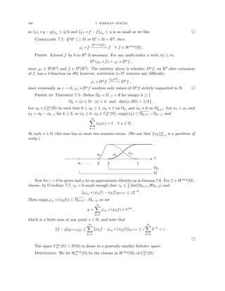
183. 7.2. EXTENSIONS FROM Ω TO Rd 183
where λ is the vector of the λj’s and e is the vector of 1’s. Now MT is a Vandermonde matrix,
and the jth row of MT c = 0 is
m+1
X
i=1
cixi−1
j = 0. Thus the polynomial p(x) =
m+1
X
i=1
cixi−1
of degree
m has m + 1 distinct roots, and so must be identically zero. This means that c = 0, and we
conclude that MT , and so also M, is nonsingular, and so the λj’s exist (uniquely, in fact).
We can generalize the Lemma through a smooth distortion of the boundary. We first define
what we mean by a smooth boundary.
Definition. For integer m ≥ 0, the domain Ω ⊂ Rd has a Cm,1-boundary (or a Lipschitz
boundary if m = 0) if there exit sets Ωj ⊂ Rd , j = 1, ..., N with N possibly +∞, with the
following properties:
(a) Ωj ⊂⊂ Rd, ∂Ω ⊂
S
j Ωj, and only finitely many of the sets intersect BR(0) for all R 0;
(b) There are functions ψj : Ωj → B1(0) that are one-to-one and onto such that both ψj
and ψ−1
j are of class Cm,1, i.e., ψj ∈ Cm,1(Ωj) and ψ−1
j ∈ Cm,1(B1(0));
(c) ψj(Ωj ∩ Ω) = B+ ≡ B1(0) ∩ Rd
+ and ψj(Ωj ∩ ∂Ω) = B+ ∩ ∂Rd
+.
That is, ∂Ω is covered by the Ωj, Ωj can be smoothly distorted by ψj into a ball with ∂Ω
distorted to the plane xd = 0. Note that ψ ∈ Cm,1(Ω) means that ψ ∈ Cm(Ω) and, for all
|α| = m, there is some C 0 such that
|Dα
ψ(x) − Dα
ψ(y)| ≤ C|x − y| ∀ x, y ∈ Ω ;
that is, Dαψ is Lipschitz.
Theorem 7.11. If m ≥ 0, 1 ≤ p ∞, and domain Ω ⊂ Rd has a Cm−1,1 boundary, then
there is a bounded (possibly nonlinear) extension operator
E : Wm,p
(Ω) → Wm,p
(Rd
) .
Proof. If m = 0, Ω may be any domain and we can extend by zero. If m ≥ 1, let {Ωj}N
j=1
and {ψj}N
j=1 be as in the definition of a Cm−1,1 boundary, where N = +∞ is possible. Let
Ω0 ⊂⊂ Ω be such that
Ω ⊂
N
[
j=0
Ωj .
Let {φk}M
k=1 (M possibly infinite) be a locally finite C∞ partition of unity subordinate to this
covering; that is, φk ∈ C∞(Rd), supp(φk) ⊂ Ωjk
for some jk between 0 and N, φk(x) 6= 0 for
only a finite number of k independent of x ∈ Ω, and
M
X
k=1
φk(x) = 1 ∀ x ∈ Ω .
Such a partition is relatively easy to construct (see, e.g., [Ad] or [GT] for a more general
construction, and also one of the exercises for this chapter). Then for f ∈ Wm,p(Ω), let fk =
φkf ∈ Wm,p(Ωjk
∩ Ω), which has support inside Ωjk
and can be extended by zero, maintaining
smoothness. Let E0 be the extension operator given in the lemma. If jk 6= 0,
E0(fk ◦ ψ−1
jk
) ∈ Wm,p
0 (B1(0)) ,

184. 184 7. SOBOLEV SPACES
so
E0(fk ◦ ψ−1
jk
) ◦ ψjk
∈ Wm,p
0 (Ωjk
) .
Extend this by zero to all of Rd. We define E by
Ef =
M
X
k=1
(jk=0)
φkf +
M
X
k=1
(jk6=0)
E0
(φkf) ◦ ψ−1
jk
◦ ψjk
∈ Wm,p
0
N
[
j=0
Ωj
.
Note that derivatives of Ef are in Lp(Rd) because the ψj and ψ−1
j ∈ Cm−1,1 (i.e., derivatives
up to order m of ψj and ψ−1
j are bounded), and so Ef ∈ Wm,p(Rd), Ef|Ω = f, and
kEfkWm,p(Rd) ≤ CkfkWm,p(Ω) ,
where C ≥ 0 depends on m, p, and Ω through the Ωj, ψj, and φk.
We remark that if Ω̄ ⊂⊂ Ω̃ ⊂ Rd, then we can assume that Ef ∈ Wm,p
0 (Ω̃). To see this,
take any φ ∈ C∞
0 (Ω̃) with φ ≡ 1 on Ω̄, and define a new bounded extension operator by φEf.
Many generalizations of this result are possible. In 1961, Calderón gave a proof assuming
only that Ω is Lipschitz. In 1970, Stein [St] gave a proof where a single operator E can be used
for any values of m and p (and Ω is merely Lipschitz). Accepting the extension to Lipschitz
domains, we have the following characterization of Wm,p(Ω).
Corollary 7.12. If Ω has a Lipschitz boundary, 1 ≤ p ∞, and m ≥ 0, then
Wm,p
(Ω) = {f|Ω : f ∈ Wm,p
(Rd
)} .
If we restrict to the Wm,p
0 (Ω) spaces, extension by 0 gives a bounded extension operator,
even if ∂Ω is ill-behaved.
Theorem 7.13. Suppose Ω ⊂ Rd, 1 ≤ p ∞, and m ≥ 0. Let E be defined on Wm,p
0 (Ω) as
the operator that extends the domain of the function to Rd by 0; that is, for f ∈ Wm,p
0 (Ω),
Ef(x) =
(
f(x) if x ∈ Ω,
0 if x /
∈ Ω.
Then E : Wm,p
0 (Ω) → Wm,p(Rd).
Of course, then
kfkWm,p
0 (Ω) = kEfkWm,p(Rd) .
Proof. If f ∈ Wm,p
0 (Ω), then there is a sequence {fj}∞
j=1 ⊂ C∞
0 (Ω) such that
fj
Wm,p(Ω)
−−
−
−
−→ f .

185. 7.3. THE SOBOLEV IMBEDDING THEOREM 185
Let φ ∈ D(Rd). Then as distributions for |α| ≤ m,
Z
Ω
Dα
fφ dx ←
Z
Ω
Dα
fjφ dx = (−1)|α|
Z
Ω
fj Dα
φ dx
→ (−1)|α|
Z
Ω
f Dα
φ dx
= (−1)|α|
Z
Rd
Ef Dα
φ dx
=
Z
Rd
Dα
Ef φ dx ,
so EDαf = DαEf in D0. The former is an L1,loc function on Rd, so the Lebesgue Lemma
(Prop. 5.7) implies that the two agree as functions. Thus
kfkWm,p(Ω) =
X
|α|≤m
Z
Rd
|EDα
f|p
dx
1/p
=
X
|α|≤m
Z
Rd
|Dα
Ef|p
dx
1/p
= kEfkWm,p(Rd) .
7.3. The Sobolev Imbedding Theorem
A measurable function f fails to lie in some Lp space either because it blows up or its tail
fails to converge to 0 fast enough (consider |x|−α near 0 or for |x| R 0). However, if Ω is
bounded and f ∈ Wm,p(Ω), m ≥ 1, the derivative is well behaved, so the function cannot blow
up as fast as an arbitrary function and we expect f ∈ Lq(Ω) for some q p.
Example. Consider Ω = (0, 1/2) and
f(x) =
1
log x
for which
f0
(x) =
−1
x(log x)2
.
The change of variable y = − log x (x = e−y) shows f ∈ W1,1(Ω). In fact, f0 ∈ Lp(Ω) only for
p = 1. But f ∈ Lp(Ω) for any p ≥ 1.
We give in this section a precise statement to this idea of trading derivatives for bounds in
higher index Lp spaces. Surprisingly, if we have enough derivatives, the function will not only
lie in L∞, but it will in fact be continuous. We begin with an important estimate.
Theorem 7.14 (Sobolev Inequality). If 1 ≤ p d and
q =
dp
d − p
,
then there is a constant C = C(d, p) such that
kukLq(Rd) ≤ Ck∇uk(Lp(Rd))d ∀ u ∈ C1
0 (Rd
) . (7.3)
Lemma 7.15 (Generalized Hölder). If Ω ⊂ Rd, 1 ≤ pi ≤ ∞ for i = 1, . . . , m, and
m
X
i=1
1
pi
= 1 ,

186. 186 7. SOBOLEV SPACES
then for fi ∈ Lpi (Ω), i = 1, . . . , m,
Z
Ω
f1(x) · · · fm(x) dx ≤ kf1kLp1 (Ω) · · · kfmkLpm (Ω) .
Proof. The case m = 1 is clear. We proceed by induction on m, using the usual Hölder
inequality. Let p0
m be conjugate to pm (i.e., 1/pm + 1/p0
m = 1), where we reorder if necessary so
pm ≥ pi ∀ i m. Then
Z
Ω
f1 · · · fm dx ≤ kf1 · · · fm−1kLp0
m
kfmkLpm
.
Now p1/p0
m, . . . , pm−1/p0
m lie in the range from 1 to ∞, and
p0
m
p1
+ · · · +
p0
m
pm−1
= 1 ,
so the induction hypothesis can be applied:
kf1 · · · fm−1kLp0
m
=
Z
|f1|p0
m · · · |fm−1|p0
m dx
1/p0
m
≤
Z
|f1|p1
dx
p0
m/p1
· · ·
Z
|fm−1|pm−1
dx
p0
m/pm−1
1/p0
m
= kf1kLp1
· · · kfm−1kLpm−1
.
Proof of the Sobolev Inequality. Let Di = ∂/∂xi, i = 1, . . . , d. We begin with the
case p = 1 d. For u ∈ C1
0 (Rd),
|u(x)| =
Z xi
−∞
Diu(x) dxi ≤
Z ∞
−∞
|Diu| dxi ∀ i ,
and so
|u(x)|d/d−1
≤
d
Y
i=1
Z ∞
−∞
|Diu| dxi
1/d−1
.
Integrate this over Rd and use generalized Hölder in each variable separately for d − 1 functions
each with Lebesgue exponent d − 1. For x1,
Z
Rd
|u(x)|d/d−1
dx ≤
Z
Rd
d
Y
i=1
Z ∞
−∞
|Diu| dxi
1/d−1
dx
=
Z
Rd−1
Z
R
Z ∞
−∞
|D1u| dx1
1/d−1 d
Y
i=2
Z ∞
−∞
|Diu| dxi
1/d−1
dx1 dx2 · · · dxd
=
Z
Rd−1
Z ∞
−∞
|D1u| dx1
1/d−1 Z
R
d
Y
i=2
Z ∞
−∞
|Diu| dxi
1/d−1
dx1 dx2 · · · dxd
≤
Z
Rd−1
Z ∞
−∞
|D1u| dx1
1/d−1 d
Y
i=2
Z
R
Z ∞
−∞
|Diu| dxi dx1
1/d−1
dx2 · · · dxd .

187. 7.3. THE SOBOLEV IMBEDDING THEOREM 187
Continuing for the other variables, we obtain
Z
Rd
|u(x)|d/d−1
dx ≤
d
Y
i=1
Z
Rd
|Diu| dx
1/d−1
.
For nonnegative numbers a1, . . . , an, the geometric mean is bounded by the arithmetic:
n
Y
i=1
ai
1/n
≤
1
n
n
X
i=1
ai ;
moreover,
n
X
i=1
ai
2
≤ n
n
X
i=1
a2
i
(i.e., in Rn, |a|`1 ≤
√
n|a|`2 ). Thus we see that
Z
Rd
|u(x)|d/d−1
dx ≤
1
d
d
X
i=1
Z
Rd
|Diu| dx
d1/d−1
=
1
d1/d−1
Z
Rd
|∇u|`1 dx
d/d−1
≤
1
d1/d−1
√
d
Z
Rd
|∇u|`2 dx
d/d−1
,
and so for Cd a constant depending on d,
kukLd/d−1
≤ Cdk∇uk(L1)d . (7.4)
For p 6= 1, we apply (7.4) to |u|γ for appropriate γ 0:
|u|γ
Ld/d−1
≤ γCd |u|γ−1
|∇u| (L1)d
≤ γCd |u|γ−1
Lp0
k∇uk(Lp)d ,
where 1/p + 1/p0 = 1. We choose γ so that
γd
d − 1
= (γ − 1)p0
;
that is
γ =
(d − 1)p
d − p
0
and so
γd
d − 1
= (γ − 1)p0
=
dp
d − p
= q .
Thus
kukγ
Lq
≤ γCdkukγ−1
Lq
k∇uk(Lp)d ,
and the result follows.
We get a better result if p d.

188. 188 7. SOBOLEV SPACES
Lemma 7.16. If p d, then there is a constant C = C(d, p) such that
kukL∞(Rd) ≤ C(diam(Ω)d
)
1
d
− 1
p k∇uk(Lp(Rd))d ∀ u ∈ C1
0 (Rd
) , (7.5)
where Ω = supp(u) and diam(Ω) is the diameter of Ω.
Proof. Suppose u ∈ C1
0 (Rd). For any unit vector e,
u(x) =
Z ∞
0
∂u
∂e
(x − re) dr =
Z ∞
0
∇u(x − re) · e dr ,
so integrate over e ∈ S1(0), the unit sphere:
dωd u(x) =
Z
S1(0)
Z ∞
0
∇u(x − re(Θ)) · e(Θ) dr dΘ
=
Z
Rd
∇u(x − y) ·
y
|y|
1
|y|d−1
dy ,
where ωd is the volume of the unit ball.
Now suppose supp(u) ⊂ B1(x). Then for 1/p + 1/p0 = 1,
|u(x)| ≤
1
dωd
k∇uk(Lp)d |y|1−d
Lp0 (B2(0))
and
|y|1−d p0
Lp0
=
Z
B2(0)
|y|(1−d)p0
dy
= dωd
Z 2
0
r(1−d)p0+d−1
dr
=
dωd
(1 − d)p0 + d
r(1−d)p0+d
2
0
∞
provided (1 − d)p0 + d 0, i.e., p d. So there is Cd,p 0 such that
|u(x)| ≤ Cd,pk∇uk(Lp)d .
If Ω = supp(u) 6⊂ B1(0), for x ∈ Ω, consider the change of variable
y =
x − x̄
diam(Ω)
∈ B1(0) ,
where x̄ is the average of x on Ω. Apply the result to
ũ(y) = u diam(Ω)y + x̄
.
We summarize and extend the two previous results in the following lemma.
Lemma 7.17. Let Ω ⊂ Rd and 1 ≤ p ∞.
(a) If 1 ≤ p d and q = dp/(d − p), then there is a constant C 0 independent of Ω such
that for all u ∈ W1,p
0 (Ω),
kukLq(Ω) ≤ Ck∇uk(Lp(Ω))d . (7.6)
(b) If p = d and Ω is bounded, then there is a constant CΩ 0 depending on the measure
of Ω such that for all u ∈ W1,d
0 (Ω),
kukLq(Ω) ≤ CΩk∇uk(Ld(Ω))d ∀ q ∞ , (7.7)
where CΩ depends also on q. Moreover, if p = d = 1, q = ∞ is allowed.

189. 7.3. THE SOBOLEV IMBEDDING THEOREM 189
(c) If d p ∞ and Ω is bounded, then there is a constant C 0 independent of Ω such
that for all u ∈ W1,p
0 (Ω),
kukL∞(Ω) ≤ C diam(Ω)d
1
d
− 1
p
k∇uk(Lp(Ω))d . (7.8)
Moreover, W1,p
0 (Ω) ⊂ C(Ω̄).
Proof. For (7.6) and (7.8), we extend (7.3) and (7.5) by density. Note that a sequence in
C∞
0 (Ω), Cauchy in W1,p
0 (Ω), is also Cauchy in Lq(Ω) if 1 ≤ p d and in C0(Ω̄) if p d, since
we can apply (7.3) or (7.5) to the difference of elements of the sequence. Moreover, when p d
and Ω bounded, the uniform limit of continuous functions in C∞
0 (Ω) ⊂ C(Ω̄) is continuous on
Ω̄, so W1,p
0 (Ω) ⊂ C(Ω̄).
Consider (7.7). The case d = 1 is a consequence of the Fundamental Theorem of Calculus and
left to the reader. Since Ω is bounded, the Hölder inequality implies Lp1 (Ω) ⊂ Lp2 (Ω) whenever
p1 ≥ p2. Thus if p = d 1 and u ∈ W1,d
0 (Ω), also u ∈ W1,p−
0 (Ω) for any 1 ≤ p− p = d. We
apply (7.6) to obtain that
kukLq(Ω) ≤ Ck∇uk(Lp− (Ω))d ≤ C|Ω|(d−p−)/d
k∇uk(Ld(Ω))d
for q ≤ dp−/(d − p−), which can be made as large as we like by taking p− close to d.
Corollary 7.18 (Poincaré). If Ω ⊂ Rd is bounded, m ≥ 0 and 1 ≤ p ∞, then the norm
on Wm,p
0 (Ω) is equivalent to
|u|Wm,p
0 (Ω) =
X
|α|=m
kDα
ukp
Lp(Ω)
1/p
.
Proof. Repeatedly use the Sobolev Inequality (7.6) (or (7.7) or (7.8) for larger p) and the
fact that Lq(Ω) ⊂ Lp(Ω) for q ≥ p.
That is, only the highest order derivatives are needed in the Wm,p
0 (Ω)-norm. This is an
important result that we will use later when studying boundary value problems.
Definition. We let
Cj
B(Ω) = {u ∈ Cj
(Ω) : Dα
u ∈ L∞(Ω) ∀ |α| ≤ j} .
This is a Banach space containing Cj(Ω̄). We come now to our main result.
Theorem 7.19 (Sobolev Imbedding Theorem). Let Ω ⊂ Rd be a domain, j ≥ 0 and m ≥ 1
integers, and 1 ≤ p ∞. The following continuous imbeddings hold.
(a) If mp ≤ d, then
Wj+m,p
0 (Ω) ,→ Wj,q
(Ω) ∀ finite q ≤
dp
d − mp
with q ≥ p if Ω is unbounded.
(b) If mp d and Ω bounded, then
Wj+m,p
0 (Ω) ,→ Cj
B(Ω) .
Moreover, if Ω has a bounded extension operator on Wj+m,p(Ω), or if Ω = Rd, then the following
hold.

190. 190 7. SOBOLEV SPACES
(c) If mp ≤ d, then
Wj+m,p
(Ω) ,→ Wj,q
(Ω) ∀ finite q ≤
dp
d − mp
with q ≥ p if Ω unbounded.
(d) If mp d then
Wj+m,p
(Ω) ,→ Cj
B(Ω) .
Proof. We begin with some remarks that simplify our task.
Note that the results for j = 0 extend immediately to the case for j 0. We claim the
results for m = 1 also extend by iteration to the case m 1. The critical exponent qm that
separates case (a) from (b), or (c) from (d), satisfies for m = 1, 2, . . . ,
qm =
dp
d − mp
which implies that for 0 ≤ k m,
qk+1 =
dp
d − (k + 1)p
=
dqk
d − qk
.
When we apply the m = 1 result successively to a series of Lebesgue exponents, we never change
case; thus, we obtain the final result for m 1.
We also claim that the results for Ω = Rd imply the results for Ω 6= Rd through the bounded
extension operator E. If u ∈ Wm,p(Ω), then Eu ∈ Wm,p(Rd) and we apply the result to Eu.
The boundedness of E allows us to restrict back to Ω. For the Wm,p
0 (Ω) spaces, we have E
defined by extension by 0 for any domain, so the argument can be applied to this case as well.
We have simplified our task to the case of Ω = Rd, m = 1, and j = 0.
Consider the case of p ≤ d, and take any v ∈ W1,p(Rd) such that kvkW1,p(Rd) ≤ 1. We wish
to apply (7.6) or (7.7) to v. To do so, we must restrict to a bounded domain and lie in W1,p
0 .
Let R = (−1, 1)d be a cube centered at 0, and R̃ = (−2, 2)d ⊃⊃ R̄. Let β ∈ Zd be any vector
with integer components. Clearly
Rd
=
[
β
(R + β) =
[
β
(R̃ + β)
is decomposed into bounded domains; however, v|R+β does not lie in W1,p
0 (R + β). Let
E : W1,p
(R) → W1,p
0 (R̃)
be a bounded extension operator with bounding constant CE. By translation we define the
extension operator
Eβ : W1,p
(R + β) → W1,p
0 (R̃ + β) ,
i.e., by
Eβ(ψ) = E(τ−βψ) = E(ψ(· − β)) .
Obviously the bounding constant for Eβ is also CE.
Now we can apply (7.6) or (7.7) to
Eβ(v|R+β)

191. 7.4. COMPACTNESS 191
to obtain, for appropriate q,
kEβ(v|R+β)kLq(R̃+β) ≤ CSk∇Eβ(v|R+β)k(Lp(R̃+β))d ,
where CS is independent of β. Thus
kvkq
Lq(R+β) ≤ kEβ(v|R+β)kq
Lq(R̃+β)
≤ Cq
Sk∇Eβ(v|R+β)kq
(Lq(R̃+β))d
≤ Cq
SCq
Ekvkq
W1,p(R+β)
≤ Cq
SCq
Ekvkp
W1,p(R+β)
,
since p ≤ q and kvkW1,p(Rd) ≤ 1. Summing over β gives
kvkLq(Rd) ≤ C
for some C 0, since the union of the R + β cover Rd a finite number of times.
If now u ∈ W1,p(Rd), u 6= 0, let
v =
u
kukW1,p(Rd)
to obtain
kukLq(Rd) ≤ CkukW1,p(Rd) ;
thus, (a) and (c) follow.
Finally the argument for p d, i.e., (b) and (d), is similar, since again our bounding constant
in (7.8) is independent of β. This completes the proof.
Remark. The extension operator need only work for W1,p(Ω), since we iterated the one
derivative case. Thus Lipschitz domains satisfy the requirements. Most domains of interest
(e.g., any polygon or polytope) have Lipschitz boundaries.
7.4. Compactness
We have an important compactness result for Sobolev spaces.
Theorem 7.20 (Rellich-Kondrachov). Let Ω ⊂ Rd be a bounded domain, 1 ≤ p ∞, and
j ≥ 0 and m ≥ 1 be integers. Then Wj+m,p
0 (Ω) is compactly imbedded in Wj,q(Ω) ∀ 1 ≤ q
dp/(d − mp) if mp ≤ d, and in Cj(Ω̄) if mp d. Moreover, if Ω ⊂ Rd has a bounded extension
operator, then a similar statement holds for Wj+m,p(Ω).
Proof. We only sketch the proof and leave it to reader to fill out the argument (more
details may be found in, e.g., [GT, p. 167–8] or [Ad, p. 144–8]). We need only show the result
for j = 0, m = 1, and W1,p
0 (Ω). The result for general j and m follows from an iteration of the
case treated. The result for Wj+m,p(Ω) can be obtained from bounded extension to Ω̃ ⊃ Ω and
the result for Wj+m,p
0 (Ω̃).
We apply the Ascoli-Arzelà Theorem 4.30 to a bounded set A in Wm,p
0 (Ω̃). By density we
may assume A ⊂ C1
0 (Ω).
First consider the case p d. The Sobolev Imbedding Theorem gives us that A is bounded
in C0(Ω̄). For equicontinuity of A, consider u ∈ A, extended by zero to Rd. Let ε 0 be given,

192. 192 7. SOBOLEV SPACES
and take any x and y such that |x − y| ε. Fix any ball B = Bε/2 of radius ε/2 containing
both x and y. In a manner similar to the proof of Lemma 7.16, we have that for z ∈ B,
u(x) − u(z) =
Z |x−z|
0
∇u(x − rez) · ez dr ,
where ez =
x − z
|x − z|
. With uB =
1
|B|
Z
B
u(x) dx, integration in z over B gives
|u(x) − uB| =
1
|B|
Z
B
Z |x−z|
0
∇u(x − rez) · ez dr dz ,
≤
1
|B|
Z
Bε(x)
Z ε
0
|∇u(x − rez)| dr dz
=
1
|B|
Z
Bε(0)
Z ε
0
|∇u(x − rz/|z|)| dr dz
=
1
|B|
Z ε
0
Z
S1(0)
Z ε
0
|∇u(x − re(Θ))| dr dΘ ρd−1
dρ
=
εd
d|B|
Z
Bε(0)
|∇u(x − z)| |z|1−d
dz
≤
εd
d|B|
k∇ukLp(Ω) k |z|1−d
kLp0 (Bε(0))
≤ Cε1−d/p
,
where p0 is the conjugate exponent to p and C is independent of x, y, u, and ε, since |B| =
ωd(ε/2)d. Now
|u(x) − u(y)| ≤ |u(x) − uB| + |u(y) − uB| ≤ 2Cε1−d/p
,
and equicontinuity of A follows for p d, and the Ascoli-Arzelà Theorem implies compactness
of A in C0(Ω̄).
Now consider the case p ≤ d, and assume initially that q = 1. For ϕ ∈ C∞
0 (B1(0)) an
approximation to the identity and ε 0, let
Aε = {u ∗ ϕε : u ∈ A} ⊂ C0
(Ω̄) .
We estimate u∗ϕε and ∇(u∗ϕε) = u∗∇ϕε using the Hölder inequality to see that Aε is bounded
and equicontinuous in C0(Ω̄) (although not uniformly so in ε). Thus Aε is precompact in C0(Ω̄)
by the Ascoli-Arzelà Theorem, and so also precompact in L1(Ω), since Ω is bounded. Next, we
estimate
Z
Ω
|u(x) − u ∗ ϕε(x)| dx ≤ ε
Z
Ω
|Du| dx ≤ Cε ,
so u ∗ ϕε is uniformly close to u in L1(Ω). It follows that A is precompact in L1(Ω) as well.
For 1 q ≤ dp/(d − p), we use Hölder and (7.6) or (7.7) to show
kukLq(Ω) ≤ Ckukλ
L1(Ω)k∇uk1−λ
(Lp(Ω))d ,
where λ + (1 − λ)(1/p − 1/d) = 1/q. Thus boundedness in W1,p
0 (Ω) and convergence in L1(Ω)
implies convergence in Lq(Ω).

193. 7.5. THE Hs SOBOLEV SPACES 193
Corollary 7.21. If Ω ⊂ Rd is bounded and has a Lipschitz boundary, 1 ≤ p ∞, and
{uj}∞
j=1 ⊂ Wj+m,p(Ω) is a bounded sequence, then there exists a subsequence {ujk
}∞
k=1 ⊂ {uj}∞
j=1
which converges in Wj,q(Ω) for q dp/(d − mp) if mp ≤ d, and in Cj(Ω̄) if mp d.
This result is often used in the following way. Suppose
uj
Wm,p(Ω)
−−
−
−
−* u as j → ∞ weakly .
Then {uj} is bounded, so there is a subsequence for which
ujk
Wm−1,p(Ω)
−
−
−
−
−
−
−
→ u as k → ∞ strongly .
7.5. The Hs Sobolev Spaces
In this section we give an alternate definition of Wm,2(Rd) = Hm(Rd) which has a natural
extension to nonintegral values of m. These fractional order spaces will be useful in the next
section on traces.
If f ∈ S(R), then
d
Df = iξ ˆ
f .
This is an example of a multiplier operator T : S → S defined by
T(f) = (m(ξ) ˆ
f(ξ))∨
,
where m(ξ), called the symbol of the operator, is in C∞(R) and has polynomial growth. For
T = D, m(ξ) = iξ. While iξ is smooth, it is not invertible, so D is a troublesome operator.
However T = 1 − D2 has
((1 − D2
)f)∧
= (1 + ξ2
) ˆ
f(ξ) ,
and (1 + ξ2) is well behaved, even though it involves two derivatives of f. What is the square
root of this operator? Let f, g ∈ S and compute using the L2-inner product:
(Tf, g) = ( c
Tf, ĝ) = ((1 + ξ2
) ˆ
f, ĝ) = ((1 + ξ2
)1/2 ˆ
f, (1 + ξ2
)1/2
ĝ) .
Thus T = S2 where
(Sf)∧
= (1 + ξ2
)1/2 ˆ
f(ξ) ,
and S is like D (S = (1 − D2)1/2).
We are thus led to consider in Rd the symbol for (I − ∆)1/2, which is
b1(ξ) = (1 + |ξ|2
)1/2
∈ S0
(Rd
) .
Then b1(ξ) is like D in Rd. For other order derivatives, we generalize for s ∈ R to
bs(ξ) = (1 + |ξ|2
)s/2
∈ S0
(Rd
) .
In fact bs(ξ) ∈ C∞(Rd) and all derivatives grow at most polynomially. Thus we can multiply
tempered distributions by bs(ξ) by Proposition 6.33.
Definition. For s ∈ R, let Λs : S0 → S0 be given by
(Λs
u)∧
(ξ) = (1 + |ξ|2
)s/2
û(ξ)
for all u ∈ S0. We call Λs the Bessel potential of order s.

194. 194 7. SOBOLEV SPACES
Remark. If u ∈ S, then
Λs
u(x) = (2π)−d/2
b̌s ∗ u(x) .
Proposition 7.22. For any s ∈ R, Λs : S0 → S0 is a continuous, linear, one-to-one, and
onto map. Moreover
Λs+t
= Λs
Λt
∀ s, t ∈ R
and
(Λs
)−1
= Λ−s
.
Definition. For s ∈ R, let
Hs
(Rd
) = {u ∈ S0
: Λs
u ∈ L2(Rd
)} ,
and for u ∈ Hs(Rd), let
kukHs = kΛs
ukL2(Rd) .
We note that Hm(Rd) has been defined previously as Wm,2(Rd). Our definitions will coincide,
as we will see.
Proposition 7.23. For all s ∈ R, k · kHs is a norm, and for u ∈ Hs,
kukHs = kΛs
ukL2 =
Z
Rd
(1 + |ξ|2
)s
|û(ξ)|2
dξ
1/2
.
Moreover, H0 = L2.
Proof. Apply the Plancherel Theorem.
Technical Lemma. For integer m ≥ 0, there are constants C1, C2 0 such that
C1(1 + x2
)m/2
≤
m
X
k=0
xk
≤ C2(1 + x2
)m/2
for all x ≥ 0.
Proof. We need constants c1, c2 0 such that
c1(1 + x2
)m
≤
m
X
k=0
xk
2
≤ c2(1 + x2
)m
∀ x ≥ 0 .
Consider
f(x) =
m
P
k=0
xk
2
(1 + x2)m
∈ C0
([0, ∞)) .
Since f(0) = 1 and limx→∞ f(x) = 1, f(x) has a maximum on [0, ∞), which gives c2. Similarly
g(x) = 1/f(x) has a maximum, giving c1.
Theorem 7.24. If m ≥ 0 is an integer, then
Hm
(Rd
) = Wm,2
(Rd
) .

195. 7.5. THE Hs SOBOLEV SPACES 195
Proof. If u ∈ Wm,2(Rd), then Dαu ∈ L2 ∀ |α| ≤ m. But then
|ξ|k
|û(ξ)| ∈ L2 ∀ k ≤ m ,
which is equivalent by the lemma to saying that
(1 + |ξ|2
)m/2
|û(ξ)| ∈ L2 .
That is, u ∈ Hm(Rd). For u ∈ Hm, we reverse the steps above to conclude that u ∈ Wm,2.
Moreover, we have shown that the norms are equivalent.
Proposition 7.25. A compatible inner product on Hs(Rd) for any s ∈ R is given by
(u, v)Hs = (Λs
u, Λs
v)L2 =
Z
Λs
uΛsv dx
for all u, v ∈ Hs(Rd). Moreover, S ⊂ Hs is dense and Hs is a Hilbert space.
Proof. It is easy to verify that (u, v)Hs is an inner product, and easily
kuk2
Hs = (u, u)Hs ∀ u ∈ Hs
.
Given ε 0 and u ∈ Hs, there is f ∈ S such that
k(1 + |ξ|2
)s/2
û − fkL2 ε ,
since S is dense in L2. But
g = (1 + |ξ|2
)−s/2
f ∈ S ,
so
ku − ǧkHs = k(1 + |ξ|2
)s/2
(û − g)kL2 ε ,
showing that S is dense in Hs. Finally, if {uj}∞
j=1 ⊂ Hs is Cauchy, then
fj = (1 + |ξ|2
)s/2
ûj
gives a Cauchy sequence in L2. Let fj
L2
−
→ f and let
g =
(1 + |ξ|2
)−s/2
f
∨
∈ Hs
.
Then
kuj − gkHs = kfj − fkL2 → 0
as j → ∞. Thus Hs is complete.
These Hilbert spaces form a one-parameter family {Hs}s∈R. They are also nested.
Proposition 7.26. If s ≥ t, then Hs ⊂ Ht is continuously imbedded.
Proof. If u ∈ Hs, then
kuk2
Ht =
Z
(1 + |ξ|2
)t
|û(ξ)|2
dξ
≤
Z
(1 + |ξ|2
)s
|û(ξ)|2
dx = kuk2
Hs .
We note that the negative index spaces are dual to the positive ones.

196. 196 7. SOBOLEV SPACES
Proposition 7.27. If s ≥ 0, then we may identify (Hs)∗ with H−s by the pairing
hu, vi = (Λs
u, Λ−s
v)L2
for all u ∈ Hs and v ∈ H−s.
Proof. By the Riesz Theorem, (Hs)∗ is isomorphic to Hs by the pairing
hu, wi = (u, w)Hs
for all u ∈ Hs and w ∈ Hs ∼
= (Hs)∗. But then
v =
(1 + |ξ|2
)s
ŵ
∨
∈ H−s
gives a one-to-one correspondence between H−s and Hs. Moreover,
kvkH−s = kwkHs ,
so we have H−s isomorphic to Hs ∼
= (Hs)∗.
Corollary 7.28. For all integral m, Hm = Wm,2.
Proof. For m ≥ 0, W−m,2 = (Wm,2
0 )∗ = (Wm,2)∗, since our domain is all of Rd.
Finally, let us consider restriction to a domain Ω ⊂ Rd.
Definition. If Ω ⊂ Rd is a domain and s ≥ 0, let
Hs
(Ω) = {u|Ω : u ∈ Hs
(Rd
)} .
Moreover, let Hs
0(Ω) be constructed as follows. Map functions in C∞
0 (Ω) to C∞
0 (Rd) by extending
by zero. Take the closure of this space in Hs(Rd). Finally, restrict back to Ω. We say more
concisely but imprecisely that Hs
0(Ω) is the completion in Hs(Rd) of C∞
0 (Ω).
Let us elaborate on our definition of Hs(Ω), s ≥ 0. We have the following general construc-
tion for a Banach space H and Z ⊂ H a closed linear subspace. We can define the quotient
space
H/Z = {x + Z : x ∈ H} ;
that is, for x ∈ H, let
x̂ = x + Z
be the coset of x, and let H/Z be the set of cosets (or equivalence classes where x, y ∈ H are
equivalent if x − y ∈ Z, so x̂ = ŷ). Then H/Z is a vector space, a norm is given by
kx̂kH/Z = inf
x̃∈H
x̃∈x̂
kx̃kH = inf
z∈Z
kx + zkH ,
and H/Z is complete. If H is a Hilbert space, the construction is simpler. Let P⊥
Z be H-
orthogonal projection onto Z⊥. Then P⊥
Z x ∈ x̂ = x + Z and
kx̂kH/Z = kP⊥
Z xkH .
We also have an inner product defined by
(x̂, ŷ)H/Z = (P⊥
Z x, P⊥
Z y)H .
If the field F = R, this is more easily computed as
(x̂, ŷ)H/Z = 1
4{kx̂ + ŷk2
H/Z − kx̂ − ŷk2
H/Z} .

197. 7.5. THE Hs SOBOLEV SPACES 197
Moreover, H/Z is a Hilbert space, isomorphic to Z⊥. We leave these facts for the reader to
verify.
For H = Hs(Rd), let
Z = {u ∈ Hs
(Rd
) : u|Ω = 0} ,
which is a closed subspace, so we have the quotient space
Hs
(Rd
)/Z = {x + Z : x ∈ Hs
(Rd
)} .
Now define
π : Hs
(Rd
)/Z → Hs
(Ω)
by
π(x̂) = π(x + Z) = x|Ω .
This map is well defined, since if x̂ = ŷ, then x|Ω = y|Ω. Moreover, π is linear, one-to-one, and
onto. So we define for x, y ∈ Hs(Ω)
kxkHs(Ω) = kπ−1
(x)kHs(Rd)/Z = inf
x̃∈Hs(Rd)
x̃|Ω=x
kx̃kHs(Rd) = kP⊥
Z xkHs(Rd) ,
and Hs(Ω) is isomorphic to Hs(Rd)/Z; that is, Hs(Ω) becomes a Hilbert space with inner
product
(x, y)Hs(Ω) = (π−1
x, π−1
y)Hs(Rd)/Z = (P⊥
Z π−1
x, P⊥
Z π−1
y)Hs(Rd) ,
which, if F = R, can be computed as
(x, y)Hs(Ω) = 1
4{kx + yk2
Hs(Ω) − kx − yk2
Hs(Ω)} .
Proposition 7.29. If Ω ⊂ Rd is a domain and s ≥ 0, then Hs(Ω) is a Hilbert space.
Moreover, for any constant C 1, given u ∈ Hs(Ω), there is ũ ∈ Hs(Rd) such that ũ|Ω = u and
kũkHs(Rd) ≤ CkukHs(Ω) ;
that is, there is a bounded extension operator E : Hs(Ω) → Hs(Rd) with kEk ≤ C.
If s = m is an integer, then we had previously defined Hm(Ω) as Wm,2(Ω). If Ω has a
Lipschitz boundary, the two definitions coincide, with equivalent, but not equal, norms. This
can be seen by considering the bounded extension operator
E : Wm,2
(Ω) → Wm,2
(Rd
) ,
for which u ∈ Wm,2(Ω) implies
kEukWm,2(Rd) ≤ CkukWm,2(Ω) ≤ CkEukWm,2(Rd) .

198. 198 7. SOBOLEV SPACES
Since Wm,2(Rd) is the same as Hm(Rd), with equivalent norms,
kukHm(Ω) = inf
v∈Hm(Rd)
v|Ω=u
kvkHm(Rd)
≤ kEukHm(Rd) ≤ C1kEukWm,2(Rd)
≤ C2kukWm,2(Ω) ≤ C2 inf
v∈Wm,2(Rd)
v|Ω=u
kvkWm,2(Rd)
≤ C3 inf
v∈Hm(Rd)
v|Ω=u
kvkHm(Rd) = C3kukHm(Ω) .
Thus our two definitions of Hm(Ω) are consistent, and, depending on the norm used, the constant
in the previous proposition may be different than described (i.e., not necessarily any C 1).
Summarizing, we have the following result.
Proposition 7.30. If Ω ⊂ Rd has a Lipschitz boundary and m ≥ 0 is an integer, then
Hm
(Ω) = Wm,2
(Ω)
and the Hm(Ω) and Wm,2(Ω) norms are equivalent.
7.6. A Trace Theorem
Given a domain Ω ⊂ Rd and a function f : Ω → R, the trace of f is its value on the
boundary of Ω; i.e., the trace is f|∂Ω, provided this makes sense. We give a precise meaning and
construction when f belongs to a Sobolev space.
We begin by restricting functions to lower dimensional hypersurfaces. Let 0 k d be an
integer, and decompose
Rd
= Rd−k
× Rk
.
If φ ∈ C0(Rd), then the restriction map
R : C0
(Rd
) → C0
(Rd−k
)
is defined by
Rφ(x0
) = φ(x0
, 0) ∀ x0
∈ Rd−k
,
wherein 0 ∈ Rk.
Theorem 7.31. Let k and d be integers with 0 k d. The restriction map R extends to
a bounded linear map from Hs(Rd) onto Hs−k/2(Rd−k), provided that s k/2.
Proof. Since S is dense in our two Sobolev spaces, it is enough to consider u ∈ S(Rd)
where R is well defined. Let v = Ru ∈ S(Rd−k).
The Sobolev norm involves the Fourier transform, so we compute for y ∈ Rd−k
v(y) = (2π)−(d−k)/2
Z
Rd−k
eiη·y
v̂(η) dη .
But, with ξ = (η, ζ) ∈ Rd−k × Rk, this is
v(y) = u(y, 0) = (2π)−d/2
Z
Rd
eiξ·(y,0)
û(ξ) dξ
= (2π)−(d−k)/2
Z
Rd−k
eiη·y
(2π)−k/2
Z
Rk
û(η, ζ) dζ
dη .

199. 7.6. A TRACE THEOREM 199
Thus
v̂(η) = (2π)−k/2
Z
Rk
û(η, ζ) dζ .
Introduce (1 + |η|2 + |ζ|2)s/2(1 + |η|2 + |ζ|2)−s/2 into the integral above and apply Hölder’s
inequality to obtain
|v̂(η)|2
≤ (2π)−k
Z
Rk
|û(η, ζ)|2
(1 + |η|2
+ |ζ|2
)s
dζ
Z
Rk
(1 + |η|2
+ |ζ|2
)−s
dζ .
The second factor on the right is
Z
Rk
(1 + |η|2
+ |ζ|2
)−s
dζ = kωk
Z ∞
0
(1 + |η|2
+ r2
)−s
rk−1
dr .
With the change of variable
(1 + |η|2
)1/2
ρ = r ,
this is
kωk(1 + |η|2
)k/2−s
Z ∞
0
(1 + ρ2
)−s
ρk−1
dρ ,
which is finite provided −2s + k − 1 −1, i.e., s k/2. Combining, we have shown that there
is a constant C 0 such that
|v̂(η)|2
(1 + |η|2
)s−k/2
≤ C2
Z
Rk
|û(η, ζ)|2
(1 + |η|2
+ |ζ|2
)s
dζ .
Integrating in η gives the bound
kvkHs−k/2(Rd−k) ≤ CkukHs(Rd) .
Thus R is a bounded linear operator mapping into Hs−k/2(Rd−k).
To see that R maps onto Hs−k/2(Rd−k), let v ∈ S(Rd−k) and extend v to ũ ∈ C∞(Rd) by
ũ(y, z) = v(y) ∀ y ∈ Rd−k
, z ∈ Rk
.
Now let ψ ∈ C∞
0 (Rk) be such that ψ(z) = 1 for |z| 1 and ψ(z) = 0 for |z| 2. Then
u(y, z) = ψ(z)ũ(y, z) ∈ S(Rd
) ,
and Ru = v. Thus R maps onto a dense subspace. Note that û(ξ) = û(η, ζ) = ψ̂(ζ)v̂(η), and a
change of variables as above leads us to kukHs(Rd) ≤ CkvkHs−k/2(Rd−k) for some C (we leave the
details to the reader). We can thus extend the result to the entire space by density.
Remark. We saw in the Sobolev Imbedding Theorem that
Hs
(Rd
) ,→ C0
B(Rd
)
for s d/2. Thus we can even restrict to a point (k = d above).
Now consider Ω ⊂ Rd such that ∂Ω is C0,1 smooth (i.e., Lipschitz). Our goal is to define
the trace of u ∈ H1(Ω) on ∂Ω. Let {Ωj}N
j=1 and {ψj}N
j=1, N possibly +∞, be as given in the
definition of a C0,1 smooth boundary. Take Ω0 open such that Ω̄0 ⊂ Ω and Ω ⊂
SN
j=0 Ωj. Let
{φk}M
k=1 be a locally finite C∞ partition of unity subordinate to the cover, so supp(φk) ⊂ Ωjk
for some jk. Define for u ∈ H1(Ω),
uk = E(φku) ◦ ψ−1
jk
: B1(0) → F ,

200. 200 7. SOBOLEV SPACES
so uk ∈ H1
0 (B1(0)). We restrict u to ∂Ω by restricting uk to S ≡ B1(0) ∩ {xd = 0}. Since
supp(uk) ⊂⊂ B1(0), we can extend by zero and apply Theorem 7.31 to obtain
kukkH1/2(S) ≤ C1kukkH1(B1(0)) .
We need to combine the uk and change variables back to Ω and ∂Ω.
Summing on k, we obtain
M
X
k=1
kukk2
H1/2(S)
≤ C1
M
X
k=1
kukk2
H1(B1(0)) ≤ C2
M
X
k=1
k(φku) ◦ ψ−1
jk
k2
H1(Rd
+)
,
using the bound on E. The final norm merely involves L2 norms of (weak) derivatives of
(φku) ◦ ψ−1. The Leibniz rule, Chain rule, and change of variables imply that each such norm
is bounded by the H1(Ω) norm of u, so
M
X
k=1
kukk2
H1/2(S)
≤ C2
M
X
k=1
k(φku) ◦ ψ−1
jk
k2
H1(Rd
+)
≤ C3kuk2
H1(Ω) .
Let the trace of u, γ0u, be defined for a.e. x ∈ ∂Ω by
γ0u(x) =
M
X
k=1
E(φku) ◦ ψ−1
jk
ψjk
(x)
.
Then we clearly have after change of variable
kγ0uk2
L2(∂Ω) ≤ C4
M
X
k=1
kukk2
L2(S) ≤ C5
M
X
k=1
kukk2
H1/2(S)
≤ C6kuk2
H1(Ω) . (7.9)
In summary, for u ∈ H1(Ω), we can define its trace γ0u on ∂Ω as a function in L2(∂Ω), and
γ0 : H1(Ω) → L2(∂Ω) is a well defined, bounded linear operator.
The above computations carry over to u ∈ Hs(Ω) for nonintegral s 1/2, as can be seen
by using the equivalent norms of the next section. Since we do not prove that those norms are
indeed equivalent, we have restricted to integral s = 1 here (and used the ordinary chain rule
rather than requiring some generalization to fractional derivatives). What we have proven is
sufficient for the next chapter, where we will use integral s.
While L2(∂Ω) is well defined (given the Lebesgue measure on the manifold ∂Ω), we do not
yet have a definition of the Sobolev spaces on ∂Ω. For s 1/2, let
Z = {u ∈ Hs
(Ω) : γ0u = 0 on ∂Ω} ;
this set is well defined by (7.9) (at least we have proven this for s ≥ 1), and is in fact closed in
Hs(Ω). We therefore define
Hs−1/2
(∂Ω) = {γ0u : u ∈ Hs
(Ω)} ⊂ L2(∂Ω) ,
which is isomorphic to Hs(Ω)/Z, which is a Hilbert space. While Hs−1/2(∂Ω) ⊂ L2(∂Ω), we
expect that such functions are in fact smoother. A norm is given by
kukHs−1/2(∂Ω) = inf
ũ∈Hs(Ω)
γ0ũ=u
kũkHs(Ω) . (7.10)
Note that this construction gives immediately the trace theorem
kγ0ukHs−1/2(∂Ω) ≤ CkukHs(Ω) ,

201. 7.6. A TRACE THEOREM 201
where C = 1. If an equivalent norm is used for Hs−1/2(∂Ω), C 6= 1 is likely. While we do
not have a constructive definition of Hs−1/2(∂Ω) and its norm that allow us to see explicitly
the smoothness of such functions, by analogy to Theorem 7.31 for Ω = Rd
+, we recognize that
Hs−1/2(∂Ω) functions have intermediate smoothness. The equivalent norm of the next section
gives a constructive sense to this statement. We summarize our results.
Theorem 7.32. Let Ω ⊂ Rd have a Lipschitz boundary. The trace operator γ0 : C0(Ω̄) →
C0(∂Ω) defined by restriction, i.e., (γ0u)(x) = u(x) ∀ x ∈ ∂Ω, extends to a bounded linear map
γ0 : Hs
(Ω)
onto
−
−
→ Hs−1/2
(∂Ω)
for any s ≥ 1 (actually, s 1/2).
We can extend this result to higher order derivatives. Tangential derivatives of γ0u are well
defined, since if Dτ is any derivative in a direction tangential to ∂Ω, then
Dτ γ0u = Dτ Eu = EDτ u = γ0Dτ u .
However, derivatives normal to ∂Ω are more delicate.
Definition. Let ν ∈ Rd be the unit outward normal vector to ∂Ω. Then for u ∈ C1(Ω̄),
Dνu =
∂u
∂ν
= ∇u · ν on ∂Ω
is the normal derivative of u on ∂Ω. If j ≥ 0 is an integer and u ∈ Cj(Ω̄), let
γju = Dj
νu =
∂ju
∂νj
.
We state and prove the following theorem for integral s = m, though it actually holds for
appropriate nonintegral values.
Theorem 7.33 (Trace Theorem). Let Ω ⊂ Rd have a Cm−1,1 ∩ C0,1 boundary for some
integer m ≥ 0. The map γ : Cm(Ω̄) → (C0(∂Ω))m+1 defined by
γu = (γ0u, γ1u, . . . , γmu)
extends to a bounded linear map
γ : Hm+1
(Ω)
onto
−
−
→
m
Y
j=0
Hm−j+1/2
(∂Ω) .
Proof. Let u ∈ Hm+1(Ω)∩C∞(Ω̄), which is dense because of the existence of an extension
operator. Then iterate the single derivative result for γ0:
γ0u ∈ Hm+1/2
(∂Ω) , γ1u = γ0(∇u · ν) ∈ Hm−1/2
(∂Ω) ,
γ2u = γ0(∇(∇u · ν) · ν) ∈ Hm−3/2
(∂Ω) , etc.,
wherein we require ∂Ω to be smooth eventually so that derivatives of ν can be taken, and wherein
we have assumed that the vector field ν on ∂Ω has been extended locally into Ω (that this can
be done follows from the Tubular Neighborhood Theorem from topology).
To see that γ maps onto, take
v ∈
m
Y
j=0
Hm−j+1/2
(∂Ω) ∩ C∞
(∂Ω) ,

202. 202 7. SOBOLEV SPACES
and construct ṽ ∈ C∞(Ω̄) ∩ Hm(Ω) such that
γṽ = v
as follows. If ∂Ω ⊂ Rd−1 we define ṽ as a polynomial
ṽ(x0
, xd) = v0(x0
) + v1(x0
)xd + · · · +
1
m!
vm(x0
)xm
d
for x0 ∈ Rd−1 and xd ∈ R, and then multiply by a smooth test function ψ(xd) that is identically
equal to 1 near xd = 0. If ∂Ω is curved, we decompose ∂Ω and map it according to the definition
of a Cm−1,1 boundary, and then apply the above construction.
Recall that
Hm
0 (Ω) = Wm,2
0 (Ω)
is the closure of C∞
0 (Ω) in Wm,2(Ω). Since γu = 0 for u ∈ C∞
0 (Ω), the same is true for any
u ∈ Hm
0 (Ω). That is, u and its m − 1 derivatives (normal and/or tangential) vanish on ∂Ω.
Theorem 7.34. If m ≥ 1 is an integer and Ω ⊂ Rd has a Cm−1,1 boundary, then
Hm
0 (Ω) = {u ∈ Hm
(Ω) : γu = 0} = {u ∈ Hm
(Ω) : γju = 0 ∀j ≤ m − 1} = ker(γ) .
Proof. As mentioned above, Hm
0 (Ω) ⊂ ker(γ). We need to show the opposite inclusion.
Again, by a mapping argument of the Cm−1,1 boundary, we need only consider the case Ω = Rd
+.
Let
u ∈ ker(γ) ∩ C∞
0 (Rd
) ,
we saw earlier that C∞
0 (Rd) is dense in Hm(Rd
+). Let ψ ∈ C∞(R) be such that ψ(t) = 1 for
t 2 and ψ(t) = 0 for t 1. For j ≥ 1, let
ψn(t) = ψ(nt) ,
which converges to 1 on {t 0} as n → ∞. Then ψn(xd)u(x) ∈ C∞
0 (Rd
+). We claim that
ψn(xd)u(x)
Hm(Rd
+)
−
−
−
−
−
→ u(x) as n → ∞ .
If so, then u ∈ Hm
0 (Rd
+) as desired.
Let α ∈ Zd be a multi-index such that |α| ≤ m and let α = (β, `) where β ∈ Zd−1 and ` ≥ 0.
Then
Dα
(ψnu − u) = Dβ
D`
d(ψnu − u) =
`
X
k=0
`
k
D`−k
d (ψn − 1)Dβ
Dk
du ,
and we need to show that this tends to 0 in L2(Rd
+) as n → ∞. It is enough to show this for
each
D`−k
d (ψn − 1)Dβ
Dk
du = n`−k
D`−k
d (ψ − 1)|nxd
Dβ
Dk
du ,
which is clear if k = `, since the measure of {x : ψn(x) − 1 0} tends to 0. If k `, our
expression is supported in {x ∈ Rd
+ : 1
n xd 2
n }, so
kD`−k
d (ψn − 1)Dβ
Dk
duk2
L2(Rd
+)
≤ C1n2(`−k)
Z
Rd−1
Z 2/n
1/n
|Dβ
Dk
du(x0
, xd)|2
dxd dx0
.

203. 7.7. THE Ws,p(Ω) SOBOLEV SPACES 203
Taylor’s theorem implies that for x = (x0, xd) ∈ Rd and j ≤ m,
Dk
du(x0
, xd) = Dk
du(x0
, 0) + · · · +
1
(j − k − 1)!
Dj−1
d u(x0
, 0)
+
1
(j − k − 1)!
Z xd
0
(xd − t)j−k−1
Dj
du(x0
, t) dt ,
which reduces to the last term since γu = 0. Thus for j = m − |β| = ` ≤ m,
kD`−k
d (ψn − 1)Dβ
Dk
duk2
L2(Rd
+)
≤ C2n2(`−k)
Z
Rd−1
Z 2/n
1/n
Z xd
0
(xd − t)`−k−1
Dβ
D`
du(x0
, t) dt
2
dxd dx0
≤ C3n2(`−k)
n−2(`−k−1)
Z
Rd−1
Z 2/n
1/n
Z 2/n
0
|Dβ
D`
du(x0
, t)| dt
2
dxd dx0
≤ C4n2
Z
Rd−1
1
n2
Z 2/n
0
|Dβ
D`
du(x0
, t)|2
dt dx0
→ 0 as n → ∞
since the measure of the inner integral tends to 0. Thus the claim is established and the proof
is complete.
7.7. The Ws,p(Ω) Sobolev Spaces
We can generalize some of the L2(Ω) results of the last two sections to Lp(Ω), and the results
for integral numbers of derivatives to nonintegral. We summarize a few of the important results.
See [Ad] for details and precise statements.
Definition. Suppose Ω ⊂ Rd, 1 ≤ p ≤ ∞, and s 0 such that s = m + σ where 0 σ 1
and m is an integer. Then we define for a smooth function u,
kukWs,p(Ω) =
kukp
Wm,p(Ω) +
X
|α|=m
Z
Ω
Z
Ω
|Dαu(x) − Dαu(y)|p
|x − y|d+σp
dx dy
1/p
if p ∞, and otherwise
kukWs,∞(Ω) = max
kukWm,∞(Ω), max
|α|=m
ess sup
x,y∈Ω
|Dαu(x) − Dαu(y)|
|x − y|σ
.
Proposition 7.35. For any 1 ≤ p ≤ ∞, k · kWs,p(Ω) is a norm.
Definition. We let Ws,p(Ω) be the completion of C∞(Ω) under the k · kWs,p(Ω)-norm, and
Ws,p
0 (Ω) is the completion of C∞
0 (Ω).
Proposition 7.36. If Ω = Rd or Ω has a Lipschitz boundary, then
Ws,2
(Ω) = Hs
(Ω) and Ws,2
0 (Ω) = Hs
0(Ω) .
Thus we have an equivalent norm on Hs(Ω) given above.
If 1 ≤ p ∞ and m = s is nonintegral, then we have analogues of the Sobolev Imbedding
Theorem, the Rellich-Kondrachov Theorem, and the Trace Theorem. For the Trace Theorem,
every time a trace is taken on a hypersurface of one less dimension (as from Ω to ∂Ω), 1/p
derivative is lost, rather than 1/2.

204. 204 7. SOBOLEV SPACES
7.8. Exercises
1. Prove that for f ∈ H1(Rd), kfkH1(Rd) is equivalent to
Z
Rd
(1 + |ξ|2
)| ˆ
f(ξ)|2
dξ
1/2
.
Can you generalize this to Hk(Rd)?
2. Prove that if f ∈ H1
0 (0, 1), then there is some constant C 0 such that
kfkL2(0,1) ≤ Ckf0
kL2(0,1) .
If instead f ∈ {g ∈ H1(0, 1) :
R 1
0 g(x) dx = 0}, prove a similar estimate.
3. Prove that δ0 6∈ (H1(Rd))∗ for d ≥ 2, but that δ0 ∈ (H1(R))∗. You will need to define what
δ0 applied to f ∈ H1(R) means.
4. Prove that H1(0, 1) is continuously imbedded in CB(0, 1). Recall that CB(0, 1) is the set of
bounded and continuous functions on (0, 1).
5. Suppose that Ω ⊂ Rd is a bounded set and {Uj}N
j=1 is a finite collection of open sets in Rd
that cover the closure of Ω (i.e., Ω̄ ⊂
N
[
j=1
Uj). Prove that there exists a finite C∞ partition
of unity in Ω subordinate to the cover. That is, construct {φk}M
k=1 such that φk ∈ C∞
0 (Rd),
φk ⊂ Ujk
for some jk, and
M
X
k=1
φk(x) = 1 .
6. Suppose that Ω ⊂ Rd is a domain and {Uα}α∈I is a collection of open sets in Rd that cover Ω
(i.e., Ω ⊂
[
α∈I
Uα). Prove that there exists a locally finite partition of unity in Ω subordinate
to the cover. That is, there exists a sequence {ψj}∞
j=1 ⊂ C∞
0 (Rd) such that
(i) For every K compactly contained in Ω, all but finitely many of the ψj vanish on K.
(ii) Each ψj ≥ 0 and
∞
X
j=1
ψj(x) = 1 for every x ∈ Ω.
(iii) For each j, the support of ψj is contained in some Uαj , αj ∈ I.
Hints: Let S be a countable dense subset of Ω (e.g., points with rational coordinates).
Consider the countable collection of balls B = {Br(x) ⊂ Rd : r is rational, x ∈ S, and
Br(x) ⊂ Uα for some α ∈ I}. Order the balls and construct on Bj = Brj (xj) a function
φj ∈ C∞
0 (Bj) such that 0 ≤ φj ≤ 1 and φj = 1 on Brj/2(xj). Then ψ1 = φ1 and ψj =
(1 − φ1)...(1 − φj−1)φj should work.
7. Let u ∈ D0(Rd) and φ ∈ D(Rd). For y ∈ Rd, the translation operator τy is defined by
τyφ(x) = φ(x − y).
(a) Show that
u(τyφ) − u(φ) =
Z 1
0
d
X
j=1
yj
∂u
∂xj
(τtyφ) dt.

205. 7.8. EXERCISES 205
(b) Apply this to
f ∈ W1,1
loc (Rd
) =
f ∈ L1,loc(Rd
) :
∂f
∂xj
∈ L1,loc(Rd
) for all j
to show that
f(x + y) − f(x) =
Z 1
0
y · ∇f(x + ty) dt.
(c) Let the locally Lipschitz functions be defined as
C0,1
loc (Rd
) = {f ∈ C0
(Rd
) : ∀R 0, there is some LR,f depending on R and f
such that |f(x) − f(y)| ≤ LR,f |x − y| ∀x, y ∈ BR(0)} .
Conclude that W1,1
loc (Rd) ⊂ C0,1
loc (Rd).
8. Counterexamples.
(a) No imbedding of W1,p(Ω) ,→ Lq(Ω) for 1 ≤ p d and q dp/(d − p). Let Ω ⊂ Rd be
bounded and contain 0, and let f(x) = |x|α. Find α so that f ∈ W1,p(Ω) but f 6∈ Lq(Ω).
(b) No imbedding of W1,p(Ω) ,→ C0
B(Ω) for 1 ≤ p d. Note that in the previous case, f is
not bounded. What can you say about which (negative) Sobolev spaces the Dirac mass lies
in?
(c) No imbedding of W1,p(Ω) ,→ L∞(Ω) for 1 p = d. Let Ω ⊂ Rd = BR(0) and let
f(x) = log(log(4R/|x|)). Show f ∈ W1,p(BR(0)).
(d) C∞ ∩ W1,∞ is not dense in W1,∞. Show that if Ω = (−1, 1) and u(x) = |x|, then
u ∈ W1,∞ but u(x) is not the limit of C∞ functions in the W1,∞-norm.
9. Suppose that fj ∈ H2(Ω) for j = 1, 2, ..., fj
w
* f weakly in H1(Ω), and Dαfj
w
* gα weakly
in L2(Ω) for all multi-indices α such that |α| = 2. Show that f ∈ H2(Ω), Dαf = gα, and,
for a subsequence, fj → f strongly in H1(Ω).
10. Suppose that Ω ⊂ Rd is bounded with a Lipschitz boundary and fj
w
* f and gj
w
* g weakly
in H1(Ω) . Show that, for a subsequence, ∇(fjgj) → ∇(fg) as a distribution. Find all p in
[1, ∞] such that the convergence can be taken weakly in Lp(Ω).
11. Suppose that Ω ∈ Rd is a bounded domain with Lipschitz boundary and {uk} ⊂ H2+(Ω) is
a bounded sequence, where 0.
(a) Show that there is u ∈ H2(Ω) such that, for a subsequence, uj → u in H2(Ω).
(b) Find all q and s ≥ 0 such that, for a subsequence, uj → u in Ws,q(Ω).
(c) For a subsequence, |uj|r∇uj → |u|r∇u in L2(Ω) for certain r ≥ 1. For fixed d, how big
can r be? Justify your answer.
12. Prove that Hs(Rd) is imbedded in C0
B(Rd) if s d/2 by completing the following outline.
(a) Show that
Z
Rd
(1 + |ξ|2
)−s
dξ ∞.
(b) If φ ∈ S and x ∈ Rd, write φ(x) as the Fourier inversion integral of φ̂. Introduce
1 = (1 + |ξ|2)s/2(1 + |ξ|2)−s/2 into the integral and apply Hölder to obtain the result for
Schwartz class functions.

206. 206 7. SOBOLEV SPACES
(c) Use density to extend the above result to Hs(Rd).
13. Interpolation inequalities.
(a) Show that for f ∈ H1(Rd) and 0 ≤ s ≤ 1, kfkHs(Rd) ≤ kfks
H1(Rd)
kfk1−s
L2(Rd)
. Can you
generalize this result to f ∈ Hr(Rd) for r 0?
(b) If Ω is bounded and ∂Ω is smooth, show that there is a constant C such that for all
f ∈ H1(Ω), kfkL2(∂Ω) ≤ Ckfk
1/2
H1(Ω)
kfk
1/2
L2(Ω)
. [Hint: Show for d = 1 on (0, 1) by considering
f(0)2
= f(x)2
−
Z x
0
d
dx
f(t)2
dt .
For d 1, flatten out ∂Ω and use a (d = 1)-type proof in the normal direction.]
14. Suppose f ∈ L2(R) and ω̂(ξ) =
p
|ξ|. Make sense of the definition g = ω ∗ f, and determine
s such that g ∈ Hs(R).
15. Suppose that ω ∈ L1(R), ω(x) 0, and ω is even. Moreover, for x 0, ω ∈ C2[0, ∞),
ω0(x) 0, and ω00(x) 0. Consider the following equation for u:
ω ∗ u − u00
= f ∈ L2(R).
(a) Show that ω̂(ξ) 0. [Hint: use that ω is even, integrate by parts, and consider subin-
tervals of size 2π/|ξ|.]
(b) Find a fundamental solution to the differential equation (i.e., replace f by δ0). You may
leave your answer in terms of an inverse Fourier Transform.
(c) For the original problem, find the solution operator as a convolution operator.
(d) Show that the solution u ∈ H2(R).
16. Elliptic regularity theory shows that if the domain Ω ⊂ Rd has a smooth boundary and
f ∈ Hs(Ω), then −∆u = f in Ω, u = 0 on ∂Ω, has a unique solution u ∈ Hs+2. For what
values of s will u be continuous? Can you be sure that a fundamental solution is continuous?
The answers depend on d.

207. CHAPTER 8
Boundary Value Problems
We consider in this chapter certain partial differential equations (PDE’s) important in science
and engineering. Our equations are posed on a bounded Lipschitz domain Ω ⊂ Rd, where
typically d is 1, 2, or 3. We also impose auxiliary conditions on the boundary ∂Ω of the domain,
called boundary conditions (BC’s). A PDE together with its BC’s constitute a boundary value
problem (BVP). We tacitly assume throughout most of this chapter that the underlying field
F = R.
It will be helpful to make the following remark before we begin. The Divergence Theorem
implies that for vector ψ ∈ (C1(Ω̄))d and scalar φ ∈ C1(Ω̄),
Z
Ω
∇ · (φψ) dx =
Z
∂Ω
φψ · ν dσ(x) , (8.1)
where ν is the unit outward normal vector (which is defined almost everywhere on the boundary
of a Lipschitz domain) and dσ is the (d − 1)-dimensional measure on ∂Ω. Since
∇ · (φψ) = ∇φ · ψ + φ ∇ · ψ ,
we have the integration-by-parts formula in Rd
Z
Ω
φ ∇ · ψ dx = −
Z
Ω
∇φ · ψ dx +
Z
∂Ω
φψ · ν dσ(x) . (8.2)
By density, we extend this formula immediately to the case where merely φ ∈ H1(Ω) and
ψ ∈ (H1(Ω))d. Note that the Trace Theorem 7.33 gives meaning to the boundary integral.
8.1. Second Order Elliptic Partial Differential Equations
Let Ω ⊂ Rd be some bounded Lipschitz domain. The general second order elliptic PDE in
divergence form for the unknown function u is
−∇ · (a∇u + bu) + cu = f in Ω , (8.3)
where a is a d × d matrix, b is a d-vector, and c and f are functions. To be physically relevant
and mathematically well posed, it is often the case that c ≥ 0, |b| is not too large (in a sense to
be made clear later), and the matrix a is uniformly positive definite, as defined below.
Definition. If Ω ⊂ Rd is a domain and a : Ω̄ → Rd×d is a matrix, then a is positive definite
if for a.e. x ∈ Ω̄,
ξT
a(x)ξ 0 ∀ξ ∈ Rd
, ξ 6= 0 ,
and a is merely positive semidefinite if only ξT a(x)ξ ≥ 0. Moreover, a is uniformly positive
definite if there is some constant a∗ 0 such that for a.e. x ∈ Ω̄,
ξT
a(x)ξ ≥ a∗|ξ|2
∀ξ ∈ Rd
.
207

208. 208 8. BOUNDARY VALUE PROBLEMS
We remark that positive definiteness of a insures that
a∇u · ∇u ≥ 0 .
The positivity of this term can be exploited mathematically. It is also related to physical
principles. In many applications, ∇u is the direction of a force and a∇u is the direction of a
response. Positive definiteness says that the response is generally in the direction of the force,
possibly deflected a bit, but never more than 90◦.
8.1.1. Practical examples. We provide some examples of systems governed by (8.3).
Example (Steady-state conduction of heat). Let Ω ⊂ R3 be a solid body, u(x) the temper-
ature of the body at x ∈ Ω, and f(x) an external source or sink of heat energy. The heat flux
is a vector in the direction of heat flow, with magnitude given as the amount of heat energy
that passes through an infinitesimal planar region orthogonal to the direction of flow divided by
the area of the infinitesimal region, per unit time. Fourier’s Law of Heat Conduction says that
the heat flux is −a∇u, where a(x), the thermal conductivity of the body, is positive definite.
Thus, heat flows generally from hot to cold. Finally, s(x) is the specific heat of the body; it
measures the amount of heat energy that can be stored per unit volume of the body per degree
of temperature. The physical principle governing the system is energy conservation. If V ⊂ Ω,
then the total heat inside V is
R
V su dx. Changes in time in this total must agree with the
external heat added due to f minus the heat lost due to movement through ∂V ; thus,
d
dt
Z
V
su dx =
Z
V
f dx −
Z
∂V
(−a∇u) · ν dσ(x) ,
where, as always, ν is the outer unit normal vector. Applying the Divergence Theorem, the last
term is
Z
∂V
a∇u · ν dσ(x) =
Z
V
∇ · (a∇u) dx ,
and so, assuming the derivative may be moved inside the integral,
Z
V
∂su
∂t
− ∇ · (a∇u)
dx =
Z
V
f dx .
This holds for every V ⊂ Ω with a reasonable boundary. By a modification of Lebesgue’s
Lemma, we conclude that, except on a set of measure zero,
∂(su)
∂t
− ∇ · (a∇u) = f . (8.4)
In steady-state, the time derivative vanishes, and we have (8.3) with b = 0 and c = 0. But
suppose that f(x) = f(u(x), x) depends on the temperature itself; that is, the external world
will add or subtract heat at x depending on the temperature found there. For example, a room
Ω may have a thermostatically controlled heater/air conditioner f = F(u, x). Suppose further
that F(u, x) = c(x)(uref(x) − u) for some c ≥ 0 and reference temperature uref(x). Then
∂(su)
∂t
− ∇ · (a∇u) = c(uref − u) , (8.5)
and, in steady-state, we have (8.3) with b = 0 and f = curef. Note that if c ≥ 0 and u ≤ uref,
then F ≥ 0 and heat energy is added, tending to increase u. Conversely, if u ≥ uref, u tends
to decrease. In fact, in time, u → uref. However, if c 0, we have a potentially unphysical
situation, in which hot areas (i.e., u uref) tend to get even hotter and cold areas even colder.
The steady-state configuration would be to have u = +∞ in the hot regions and u = −∞ in the

209. 8.1. SECOND ORDER ELLIPTIC PARTIAL DIFFERENTIAL EQUATIONS 209
cold regions! Thus c ≥ 0 should be demanded on physical grounds (later it will be required on
mathematical grounds as well).
Example (The electrostatic potential). Let u be the electrostatic potential, for which the
electric flux is −a∇u for some a measuring the electrostatic permitivity of the medium Ω.
Conservation of charge over an arbitrary volume in Ω, the Divergence Theorem, and the Lebesgue
Lemma give (8.3) with c = 0 and b = 0, where f represents the electrostatic charges.
Example (Steady-state fluid flow in a porous medium). The equations of steady-state flow
of a nearly incompressible, single phase fluid in a porous medium are similar to those for the
flow of heat. In this case, u is the fluid pressure. Darcy’s Law gives the volumetric fluid flux
(also called the Darcy velocity) as −a(∇u − gρ), where a is the permeability of the medium Ω
divided by the fluid viscosity, g is the gravitational vector, and ρ is the fluid density. The total
mass in volume V ⊂ Ω is
R
V ρ dx, and this quantity changes in time due to external sources (or
sinks, if negative, such as wells) represented by f and mass flow through ∂V . The mass flux is
given by multiplying the volumetric flux by ρ. That is, with t being time,
d
dt
Z
V
ρ dx =
Z
V
f dx −
Z
∂V
−ρa(∇u − gρ) · ν dσ(x)
=
Z
V
f dx +
Z
V
∇ · [ρa(∇u − gρ)] dx ,
and we conclude that, provided we can take the time derivative inside the integral,
∂ρ
∂t
− ∇ · [ρa(∇u − gρ)] = f .
Generally speaking, ρ = ρ(u) depends on the pressure u through an equation-of-state, so this
is a time dependent, nonlinear equation. If we assume steady-state flow, we can drop the first
term. We might also simplify the equation-of-state if ρ(u) ≈ ρ0 is nearly constant (at least over
the pressures being encountered). One choice uses
ρ(u) ≈ ρ0 + γ(u − u0) ,
where γ and u0 are fixed (note that these are the first two terms in a Taylor approximation of
ρ about u0). Substituting this in the equation above results in
−∇ · {a[(ρ0 + γ(u − u0))∇u − g(ρ0 + γ(u − u0))2
]} = f .
This is still nonlinear, so a further simplification would be to linearize the equation (i.e., assume
u ≈ u0 and drop all higher order terms involving u − u0). Since ∇u = ∇(u − u0), we obtain
finally
−∇ · {ρ0a[∇u − g(ρ0 + 2γ(u − u0))]} = f ,
which is (8.3) with a replaced by ρ0a, c = 0, b = −2ρ0agγ, and f replaced by f − ∇ · [ρ0ag(ρ0 −
2γu0)].
8.1.2. Boundary conditions (BC’s). In each of the previous examples, we determined
the equation governing the behavior of the system, given the external forcing term f distributed
over the domain Ω. However, the description of each system is incomplete, since we must also
describe the external interaction with the world through its boundary ∂Ω.
These boundary conditions generally take one of three forms, though many others are possi-
ble depending on the system being modeled. Let ∂Ω be decomposed into ΓD, ΓN , and ΓR, where
the three parts of the boundary are open, contained in ∂Ω, cover ∂Ω (i.e., ∂Ω = Γ̄D ∪ Γ̄N ∪ Γ̄R),

210. 210 8. BOUNDARY VALUE PROBLEMS
and are mutually disjoint (so ΓD ∩ ΓN = ΓD ∩ ΓR = ΓN ∩ ΓR = ∅). We specify the boundary
conditions as
u = uD on ΓD , (8.6)
−(a∇u + bu) · ν = gN on ΓN , (8.7)
−(a∇u + bu) · ν = gR(u − uR) on ΓR , (8.8)
where uD, uR, gN , and gR are functions with gR 0. We call (8.6) a Dirichlet BC, (8.7) a
Neumann BC, and (8.8) a Robin BC.
The Dirichlet BC fixes the value of the (trace of) the unknown function. In the heat con-
duction example, this would correspond to specifying the temperature on ΓD.
The Neumann BC fixes the normal component of the flux −(a∇u + bu) · ν. The PDE
controls the tangential component, as this component of the flux does not leave the domain in
an infinitesimal sense. However, the normal component is the flux into or out of the domain,
and so it may be fixed in certain cases. In the heat conduction example, gN = 0 would represent
a perfectly insulated boundary, as no heat flux may cross the boundary. If instead heat is added
to (or taken away from) the domain through some external heater (or refrigerator), we would
specify this through nonzero gN .
The Robin BC is a combination of the first two types. It specifies that the flux is proportional
to the deviation of u from uR. If u = uR, there is no flux; otherwise, the flux tends to drive u
to uR, since gR 0 and a is positive definite. This is a natural boundary condition for the heat
conduction problem when the external world is held at a fixed temperature uR and the body
adjusts to it. We will no longer discuss the Robin condition, but instead concentrate on the
Dirichlet and Neumann BC’s.
The PDE (8.3) and the BC’s (8.6)–(8.8) constitute our boundary value problem (BVP). As
we will see, this problem is well posed, which means that there exists a unique solution to the
system, and that it varies continuously in some norm with respect to changes in the data f, uD,
and gN .
8.2. A Variational Problem and Minimization of Energy
For ease of exposition, let us consider the Dirichlet BVP
−∇ · (a∇u) + cu = f in Ω ,
u = uD on ΓD ,
(8.9)
where we have set b = 0 and ΓD = ∂Ω. To make classical sense of this problem, we would expect
u ∈ C2(Ω) ∩ C0(Ω̄), so we would need to require that f ∈ C0(Ω), a ∈ (C1(Ω))d×d, c ∈ C0(Ω),
and uD ∈ C0(∂Ω). Often in practice these functions are not so well behaved, so we therefore
interpret the problem in a weak or distributional sense.
If merely f ∈ L2(Ω), a ∈ (W1,∞(Ω))d×d, and c ∈ L∞(Ω), then we should expect u ∈ H2(Ω).
Moreover, then u|∂Ω ∈ H3/2(∂Ω) is well defined by the trace theorem. Thus the BVP has a
mathematically precise and consistent meaning formulated as: If f, a, and c are as stated and
uD ∈ H3/2(∂Ω), then find u ∈ H2(Ω) such that (8.9) holds. This is not an easy problem;
fortunately, we can find a better formulation using ideas of duality from distribution theory.
We first proceed formally: we will justify the calculations a bit later. We first multiply the
PDE by a test function v ∈ D(Ω), integrate in x, and integrate by parts. This is
Z
Ω
(−∇ · (a∇u) + cu) v dx =
Z
Ω
(a∇u · ∇v + cuv) dx =
Z
Ω
fv dx .

211. 8.2. A VARIATIONAL PROBLEM AND MINIMIZATION OF ENERGY 211
We have evened out the required smoothness of u and v, requiring only that each has a single
derivative. Now if we only ask that f ∈ H−1(Ω), a ∈ (L∞(Ω))d×d, and c ∈ L∞(Ω), then
we should expect that u ∈ H1(Ω); moreover, we merely need v ∈ H1
0 (Ω). This is much less
restrictive than asking for u ∈ H2(Ω), so it should be easier to find such a solution satisfying
the PDE. Moreover, u|∂Ω ∈ H1/2(∂Ω) is still a nice function, and only requires uD ∈ H1/2(∂Ω).
Remark. Above we wanted to take cu in the same space as f, which was trivially achieved
for c ∈ L∞(Ω). The Sobolev Imbedding Theorem allows us to do better. For example, suppose
indeed that u ∈ H1(Ω) and that we want cu ∈ L2(Ω) (to avoid negative index spaces). Then in
fact u ∈ Lq(Ω) for any finite q ≤ 2d/(d − 2) if d ≥ 2 and u ∈ CB(Ω) ⊂ L∞(Ω) if d = 1. Thus we
can take
c ∈





L2(Ω) if d = 1 ,
L2+(Ω) if d = 2 for any 0 ,
Ld if d ≥ 3 ,
and obtain cu ∈ L2(Ω) as desired.
With this reduced regularity requirement on u (u ∈ H1(Ω), not H2(Ω)), we can reformulate
the problem rigorously as a variational problem. Our PDE (8.9) involves a linear operator
A ≡ −∇ · a∇ + c : H1
(Ω) → H−1
(Ω) ,
which we will transform into a bilinear operator
B : H1
(Ω) × H1
(Ω) → R .
Assume that u ∈ H1(Ω) solves the PDE (we will show existence of a solution later), and take a
test function v ∈ H1
0 (Ω). Then
h−∇ · (a∇u) + cu, viH−1,H1
0
= hf, viH−1,H1
0
.
Let {vj}∞
j=1 ⊂ D(Ω) be a sequence converging to v in H1
0 (Ω). Then
h−∇ · (a∇u), viH−1,H1
0
= lim
j→∞
h−∇ · a∇u, vjiH−1,H1
0
= lim
j→∞
h−∇ · a∇u, vjiD0,D
= lim
j→∞
ha∇u, ∇vjiD0,D
= lim
j→∞
(a∇u, ∇vj)L2(Ω)
= (a∇u, ∇v)L2(Ω) ,
where the “L2(Ω)”-inner product is actually the one for (L2(Ω))d. Thus
(a∇u, ∇v)L2(Ω) + (cu, v)L2(Ω) = hf, viH−1,H1
0
.
Let us define B by
B(u, v) = (a∇u, ∇v)L2(Ω) + (cu, v)L2(Ω) ∀u, v ∈ H1
(Ω) ,
and F : H1
0 (Ω) → R by
F(v) = hf, viH−1,H1
0
,
then the PDE has been reduced to the variational problem:
Find u ∈ H1(Ω) such that
B(u, v) = F(v) ∀v ∈ H1
0 (Ω) .

212. 212 8. BOUNDARY VALUE PROBLEMS
What about the boundary condition? Recall that the trace operator
γ0 : H1
(Ω)
onto
−→ H1/2
(∂Ω) .
Thus there is some ũD ∈ H1(Ω) such that γ0(ũD) = uD ∈ H1/2(∂Ω). It is therefore required
that
u ∈ H1
0 (Ω) + ũD ,
so that γ0(u) = γ0(ũD) = uD. For convenience, we no longer distinguish between uD and its
extension ũD. We summarize our construction below.
Theorem 8.1. If Ω ⊂ Rd is a domain with a Lipschitz boundary, and f ∈ H−1(Ω), a ∈
(L∞(Ω))d×d, c ∈ L∞(Ω), and uD ∈ H1(Ω), then the BVP for u ∈ H1(Ω),
−∇ · (a∇u) + cu = f in Ω ,
u = uD on ∂Ω ,
(8.10)
is equivalent to the variational problem:
Find u ∈ H1
0 (Ω) + uD such that
B(u, v) = F(v) ∀v ∈ H1
0 (Ω) , (8.11)
where B : H1(Ω) × H1(Ω) → R is
B(u, v) = (a∇u, ∇v)L2(Ω) + (cu, v)L2(Ω)
and F : H1
0 (Ω) → R is
F(v) = hf, viH−1(Ω),H1
0 (Ω) .
Actually, we showed that a solution to the BVP (8.10) gives a solution to the variational
problem (8.11). By reversing the steps above, we see the converse implication. Note also that
above we have extended the integration by parts formula (8.2) to the case where φ = v ∈ H1
0 (Ω)
and merely ψ = −a∇u ∈ (L2(Ω))d.
The connection between the BVP (8.10) and the variational problem (8.11) is further illu-
minated by considering the following energy functional.
Definition. If a symmetric (i.e., a = aT ), then the energy functional J : H1
0 (Ω) → R for
(8.10) is given by
J(v) = 1
2
(a∇v, ∇v)L2(Ω) + (cv, v)L2(Ω)
− hf, viH−1(Ω),H1
0 (Ω) + (a∇uD, ∇v)L2(Ω) + (cuD, v)L2(Ω) .
(8.12)
We will study the calculus of variations in Chapter 9; however, we can easily make a simple
computation here. We claim that any solution of (8.10), minus uD, minimizes the “energy”
J(v). To see this, let v ∈ H1
0 (Ω) and compute
J(u − uD + v) − J(u − uD) = (a∇u, ∇v)L2(Ω) + (cu, v)L2(Ω) − hf, viH−1(Ω),H1
0 (Ω)
+ 1
2
(a∇v, ∇v)L2(Ω) + (cv, v)L2(Ω)
,
(8.13)
using that a is symmetric. If u satisfies (8.11), then
J(u − uD + v) − J(u − uD) = 1
2
(a∇v, ∇v)L2(Ω) + (cv, v)L2(Ω)
≥ 0 ,
provided that a is positive definite and c ≥ 0. Thus every function in H1
0 (Ω) has “energy” at
least as great as u − uD.

213. 8.3. THE CLOSED RANGE THEOREM AND OPERATORS BOUNDED BELOW 213
Conversely, if u − uD ∈ H1
0 (Ω) is to minimize the energy J(v), then replacing in (8.13) v by
v for ∈ R, 6= 0, we see that the difference quotient
1
J(u − uD + v) − J(u − uD)
= (a∇u, ∇v)L2(Ω) + (cu, v)L2(Ω) − hf, viH−1(Ω),H1
0 (Ω)
+
2
(a∇v, ∇v)L2(Ω) + (cv, v)L2(Ω)
,
(8.14)
must be nonnegative if 0 and nonpositive if 0. Taking → 0 on the right-hand side
shows that the first three terms must be both nonnegative and nonpositive, i.e., zero; thus, u
must satisfy (8.11). Note that as → 0, the left-hand side is a kind of derivative of J at u − uD.
At the minimum, we have a critical point where the derivative vanishes.
Theorem 8.2. If the hypotheses of Theorem 8.1 hold, and if c ≥ 0 and a is symmetric and
positive definite, then (8.10) and (8.11) are also equivalent to the minimization problem:
Find u ∈ H1
0 (Ω) + uD such that
J(u − uD) ≤ J(v) ∀v ∈ H1
0 (Ω) , (8.15)
where J is given above by (8.12).
The physical principles of conservation or energy minimization are equivalent in this context,
and they are connected by the variational problem: (1) it is the weak form of the BVP, given
by multiplying by a test function, integrating, and integrating by parts to even out the number
of derivatives on the solution and the test function, and (2) the variational problem also gives
the critical point of the energy functional where it is minimized.
Example. As another example of the use of energy functionals, consider a thin membrane
stretched over a rigid frame. We describe this as follows. Let Ω ∈ R2 be open in the xy-plane
and suppose that there is a function f : ∂Ω → R which describes the z-coordinate (height) of
the rigid frame. That is, the frame is
{(x, y, z) : z = f(x, y) for all (x, y) ∈ ∂Ω} .
We let u : Ω → R be the height of the membrane. The membrane will assume the shape that
minimizes the energy, subject to the constraint that it attaches to the rigid frame. If f = 0, the
energy functional E : H1(Ω) → R is a sum of the elastic energy and the gravitational potential
energy:
E(u) =
Z
Ω
[1
2a|∇u|2
+ gu] dx ,
where a is a constant related to the elasticity of the membrane and g is the gravitational constant.
We minimize E subject to the constraint that the trace of u, γ0(u), vanishes on the boundary.
This minimization problem gives rise to the partial differential equation
−∇ · a∇u = −g in Ω , u = 0 on ∂Ω ,
and, equivalently, its variational form.
8.3. The Closed Range Theorem and Operators Bounded Below
We continue with an abstract study of equation solvability that will be needed in the next
section. In this section, we do not require the field to be real. We begin with a basic definition.
Definition. Let X be a NLS and Z ⊂ X. Then the orthogonal complement of Z is
Z⊥
= {x∗
∈ X∗
: hx∗
, ziX∗,X = 0 ∀z ∈ Z} .

214. 214 8. BOUNDARY VALUE PROBLEMS
Proposition 8.3. Let X be a NLS and Z ⊂ X. Then
(a) Z⊥ is closed in X∗, and
(b) Z ⊂ (Z⊥)⊥.
Moreover, if Z ⊂ X is a linear subspace and X is reflexive, then
(c) Z is closed in X if and only if Z = (Z⊥)⊥.
Of course, (Z⊥)⊥ ⊂ X∗∗, so we have used the natural inclusion X ⊂ X∗∗ implicitly above.
Proof. For (a), suppose that we have a sequence {yj}∞
j=1 ⊂ Z⊥ that converges in X∗ to y.
But then for any z ∈ Z,
0 = hyj, ziX∗,X → hy, ziX∗,X ,
so y ∈ Z⊥ and Z⊥ is closed. Result (b) is a direct consequence of the definitions: for z ∈ Z ⊂
X ⊂ X∗∗ we want that z ∈ (Z⊥)⊥, i.e., that hz, yiX∗∗,X∗ = hz, yiX,X∗ = 0 for all y ∈ Z⊥, which
holds.
Finally, for (c), that Z is closed follows from (a). For the other implication, suppose Z is
closed. We have (b), so we only need to show that (Z⊥)⊥ ⊂ Z. Suppose that there is some
nonzero x ∈ (Z⊥)⊥ ⊂ X∗∗ = X such that x 6∈ Z. Now the Hahn-Banach Theorem, specifically
Lemma 2.33, gives us the existence of f ∈ ((Z⊥)⊥)∗ such that f(x) 6= 0 but f(z) = 0 for all
z ∈ Z, since Z is linear. That is, f ∈ Z⊥, so x cannot be in (Z⊥)⊥, a contradiction.
Proposition 8.4. Let X and Y be NLS’s and A : X → Y a bounded linear operator. Then
R(A)⊥
= N(A∗
) ,
where R(A) is the range of A and N(A∗) is the null space of A∗.
Proof. We note that y ∈ R(A)⊥ if and only if for every x ∈ X,
0 = hy, AxiY ∗,Y = hA∗
y, xiX∗,X ,
which is true if and only if A∗y = 0.
We have now immediately the following important theorem.
Theorem 8.5 (Closed Range Theorem). Let X and Y be NLS’s, Y = Y ∗∗, and A : X → Y
a bounded linear operator. Then R(A) is closed in Y if and only if R(A) = N(A∗)⊥.
This theorem has implications for a class of operators that often arise.
Definition. Let X and Y be NLS’s and A : X → Y . We say that A is bounded below if
there is some constant γ 0 such that
kAxkY ≥ γkxkX ∀x ∈ X .
A linear operator that is bounded below is one-to-one. If it also mapped onto Y , it would
have a continuous inverse. We can determine whether R(A) = Y by the Closed Range Theorem.
Theorem 8.6. Let X and Y = Y ∗∗ be Banach spaces and A : X → Y a continuous linear
operator. Then the following are equivalent:
(a) A is bounded below;
(b) A is injective and R(A) is closed;
(c) A is injective and R(A) = N(A∗)⊥.

215. 8.4. THE LAX-MILGRAM THEOREM 215
Proof. The Closed Range Theorem gives the equivalence of (b) and (c). Suppose (a). Then
A is injective. Let {yj}∞
j=1 ⊂ R(A) converge to y ∈ Y . Choose xj ∈ X so that Axj = yj (the
choice is unique), and note that
kyj − ykkY = kA(xj − xk)kY ≥ γkxj − xkkX
implies that {xj}∞
j=1 is Cauchy. Let xj → x ∈ X and define y = Ax ∈ R(A). Since A is
continuous, yj = Axj → Ax = y, and R(A) is closed.
Conversely, suppose (b). Then R(A), being closed, is a Banach space itself. Thus A : X →
R(A) is invertible, with continuous inverse by the Open Mapping Theorem 2.40. For x ∈ X,
compute
kxkX = kA−1
AxkX ≤ kA−1
kkAxkY ,
which gives (a) with constant γ = 1/kA−1k.
Corollary 8.7. Let X and Y = Y ∗∗ be Banach spaces and A : X → Y a continuous linear
operator. Then A is continuously invertible if and only if A is bounded below and N(A∗) = {0}
(i.e., A∗ is injective).
8.4. The Lax-Milgram Theorem
It is easy at this stage to prove existence of a unique solution to (8.10), or equivalently,
(8.11), provided that a is symmetric and uniformly positive definite, c ≥ 0, and both these
functions are bounded. This is because B(·, ·) is then an inner-product on H1
0 (Ω), and this
inner-product is equivalent to the usual one. To see these facts, we easily note that B is bilinear
and symmetric (since a is symmetric), and B(v, v) ≥ 0. We will show that B(v, v) = 0 implies
v = 0 in a moment, which will show that B is an inner-product. For the equivalence with the
H1
0 (Ω) inner-product, we have the upper bound
B(v, v) = (a∇v, ∇v) + (cv, v) ≤ kak(L∞(Ω))d×d k∇vk2
L2(Ω) + kckL∞(Ω)kvk2
L2(Ω) ≤ C1kvk2
H1
0 (Ω) ,
for some constant C1. A lower bound is easy to obtain if c is strictly positive, i.e., bounded
below by a positive constant. But we allow merely c ≥ 0 by using the Poincaré inequality, which
is a direct consequence of Cor. 7.18.
Theorem 8.8 (Poincaré Inequality). If Ω ⊂ Rd is bounded, then there is some constant C
such that
kvkH1
0 (Ω) ≤ Ck∇vkL2(Ω) ∀v ∈ H1
0 (Ω) . (8.16)
Now we have that
B(v, v) = (a∇v, ∇v) + (cv, v) ≥ a∗k∇vk2
L2(Ω) ≥ (a∗/C2
)kvk2
H1
0 (Ω) ,
and now both B(v, v) = 0 implies v = 0 and the equivalence of norms is established.
Problem (8.11) becomes:
Find w = u − uD ∈ H1
0 (Ω) such that
B(w, v) = F(v) − B(uD, v) ≡ F̃(v) ∀v ∈ H1
0 (Ω).
Now F̃ : H1
0 (Ω) → R is linear and bounded:
|F̃(v)| ≤ |F(v)| + |B(uD, v)| ≤ kFkH−1(Ω) + CkuDkH1(Ω)
kvkH1
0 (Ω) ,

216. 216 8. BOUNDARY VALUE PROBLEMS
where, again, C depends on the L∞(Ω)-norms of a and c. Thus F̃ ∈ (H1
0 (Ω))∗ = H−1(Ω), and
we seek to represent F̃ as w ∈ H1
0 (Ω) through the inner-product B. The Riesz Representation
Theorem 3.12 gives us a unique such w. We have proved the following theorem.
Theorem 8.9. If Ω ⊂ Rd is a Lipschitz domain, f ∈ H−1(Ω), uD ∈ H1(Ω), a ∈ (L∞(Ω))d×d
is uniformly positive definite and symmetric on Ω, and c ≥ 0 is in L∞(Ω), then there is a
unique solution u ∈ H1(Ω) to the BVP (8.10) and, equivalently, the variational problem (8.11).
Moreover, there is a constant C 0 such that
kukH1(Ω) ≤ C kFkH−1(Ω) + kuDkH1(Ω)
. (8.17)
This last inequality is a consequence of the facts that
kukH1(Ω) ≤ kwkH1
0 (Ω) + kuDkH1(Ω)
and
kwk2
H1
0 (Ω) ≤ CB(w, w) = CF̃(w) ≤ C kFkH−1(Ω) + kuDkH1(Ω)
kwkH1
0 (Ω) .
Remark. We leave it as an exercise to show that u is independent of the extension of uD
from ∂Ω to all of Ω. This extension is not unique, and we have merely that once the extension
for uD is fixed, then w is unique. That is, w depends on the extension. The reader should
show that the sum u = w + uD does not depend on the extension chosen. Moreover, since the
extension operator is bounded, that is,
kuDkH1(Ω) ≤ CkuDkH1/2(∂Ω) ,
we can modify (8.17) so that it reads
kukH1(Ω) ≤ C kFkH−1(Ω) + kuDkH1/2(∂Ω)
,
and thereby refers only to the raw data itself and not the extension.
For more general problems, where either a is not symmetric, or b 6= 0 in the original Dirichlet
problem (8.9), B is no longer symmetric, so it cannot be an inner-product. We need a gener-
alization of the Riesz theorem to handle this case. In fact, we present this generalization for
Banach spaces rather than restricting to Hilbert spaces.
Theorem 8.10 (Generalized Lax-Milgram Theorem). Let X and Y be real Banach spaces,
and suppose that Y is reflexive, B : X × Y → R is bilinear, and X ⊂ X be a closed subspace.
Assume also the following three conditions:
(a) B is continuous on X × Y , i.e., there is some M 0 such that
|B(x, y)| ≤ MkxkX kykY ∀x ∈ X, y ∈ Y ;
(b) B satisfies the inf-sup condition on X × Y , i.e., there is some γ 0 such that
inf
x∈X
kxkX =1
sup
y∈Y
kykY =1
B(x, y) ≥ γ 0 ;
(c) and B satisfies the nondegeneracy condition on X that
sup
x∈X
B(x, y) 0 ∀y ∈ Y, y 6= 0 .
If x0 ∈ X and F ∈ Y ∗, then there is a unique u solving the abstract variational problem:
Find u ∈ X + x0 ⊂ X such that
B(u, v) = F(v) ∀v ∈ Y . (8.18)

217. 8.4. THE LAX-MILGRAM THEOREM 217
Moreover,
kukX ≤
1
γ
kFkY ∗ +
M
γ
+ 1
kx0kX . (8.19)
We remark that (b) is often written equivalently as
sup
y∈Y
y6=0
B(x, y)
kykY
≥ γkxkX ∀x ∈ X .
In our context, X = H1(Ω), X = Y = H1
0 (Ω), and x0 = uD.
Proof. Assume first that x0 = 0. For each fixed x ∈ X, B(x, ·) defines a linear functional
on Y , since B is linear in each variable separately, so certainly the second. Let A represent the
operator that takes x to B(x, y):
hAx, yi = Ax(y) ≡ B(x, y) ∀x ∈ X, y ∈ Y .
Since (a) gives that
|hAx, yi| = |B(x, y)| ≤ (MkxkX )kykY ,
Ax is a continuous linear functional, i.e., A : X → Y ∗. Moreover, A itself is linear, since B is
linear in its first variable, and therefore A is a continuous linear operator:
kAxkY ∗ = sup
kykY =1
hAx, yi ≤ MkxkX .
We reformulate (8.18) in terms of A as the problem of finding u ∈ X such that
Au = F .
Now (b) implies that
kAxkY ∗ ≥ γkxkX ∀x ∈ X , (8.20)
so A is bounded below and u, if it exists, must be unique (i.e., A is one-to-one). Since X
is closed, it is a Banach space and we conclude that the range of A, R(A), is closed in Y ∗
(Theorem 8.6). The Closed Range Theorem 8.5 now implies that R(A) = N(A∗)⊥. We wish to
show that N(A∗) = {0}, so that A maps onto. Suppose that for some y ∈ Y = Y ∗∗, y ∈ N(A∗);
that is,
B(x, y) = hAx, yi = 0 ∀x ∈ X .
But (c) implies then that y = 0. So we have that A has a bounded inverse, with kA−1k ≤ 1/γ
by (8.20), and u = A−1F solves our problem.
Finally, we compute
kukX = kA−1
FkX ≤ kA−1
kkFkY ∗ ≤
1
γ
kFkY ∗ .
The theorem is established when x0 = 0.
If x0 6= 0, we reduce to the previous case, since (8.18) is equivalent to:
Find w ∈ X such that
B(w, v) = F̃(v) ∀v ∈ Y ,
where u = w + x0 ∈ X + x0 ⊂ X and
F̃(v) = F(v) − B(x0, v) .

218. 218 8. BOUNDARY VALUE PROBLEMS
Now F̃ ∈ Y ∗ and
|F̃(v)| ≤ |F(v)| + |B(x0, v)| ≤ kFkY ∗ + Mkx0kX
kvkY .
Thus the previous result gives
kwkX ≤
1
γ
kFkY ∗ + Mkx0kX
,
and so
kukX ≤ kw + x0kX ≤ kwkX + kx0kX
gives the desired bound.
When X = Y is a Hilbert space, things are a bit simpler.
Corollary 8.11 (Lax-Milgram Theorem). Let X be a real Hilbert space with closed subspace
H. Let B : X × X → R be a bilinear functional satisfying the following two conditions:
(i) B is continuous on X, i.e., there is some M 0 such that
|B(x, y)| ≤ MkxkXkykX ∀x, y ∈ X ;
(ii) B is coercive (or elliptic) on H i.e., there is some γ 0 such that
B(x, x) ≥ γkxk2
X ∀x ∈ H .
If x0 ∈ X and F ∈ H∗, then there is a unique u solving the abstract variational problem:
Find u ∈ H + x0 ⊂ X such that
B(u, v) = F(v) ∀v ∈ H . (8.21)
Moreover,
kukX ≤
1
γ
kFkH∗ +
M
γ
+ 1
kx0kX . (8.22)
Proof. The corollary is just a special case of the theorem except that (ii) has replaced (b)
and (c). We claim that (ii) implies both (b) and (c), so the corollary follows.
Easily, we have (c), since for any y ∈ H,
sup
x∈H
B(x, y) ≥ B(y, y) ≥ γkyk2
X 0
whenever y 6= 0. Similarly, for any x ∈ H with norm one,
sup
y∈H
kykX =1
B(x, y) ≥ B(x, x) ≥ γ 0 ,
so the infimum over all such x is bounded below by γ, which is (b).
The Generalized Lax-Milgram Theorem gives the existence of a bounded linear solution
operator S : Y ∗ × X → X such that S(F, x0) = u ∈ X + x0 ⊂ X satisfies
B(S(F, x0), v) = F(v) ∀v ∈ Y .
The bound on S is given by (8.19). This bound shows that the solution varies continuously with
the data. That is, by linearity,
kS(F, x0) − S(G, y0)kX ≤
1
γ
kF − GkX∗ +
M
γ
+ 1
kx0 − y0kX .
So if the data (F, x0) is perturbed a bit to (G, y0), then the solution S(F, x0) changes by a small
amount to S(G, y0), where the magnitudes of the changes are measured in the norms as above.

219. 8.5. APPLICATION TO SECOND ORDER ELLIPTIC EQUATIONS 219
8.5. Application to Second Order Elliptic Equations
We consider again the BVP (8.10), in the form of the variational problem (8.11). To apply
the Lax-Milgram Theorem, we set X = H1(Ω), X = Y = H1
0 (Ω), and x0 = uD. Now B :
H1(Ω) × H1(Ω) → R is continuous, since a and c are bounded:
|B(u, v)| = |(a∇u, ∇v)L2(Ω) + (cu, v)L2(Ω)|
≤ kak(L∞(Ω))d×d k∇ukL2(Ω)k∇vkL2(Ω) + kckL∞(Ω)kukL2(Ω)kvkL2(Ω)
≤ MkukH1(Ω)kvkH1(Ω) ,
by Hölder’s inequality for some M 0 depending on the bounds for a and c. Coercivity is more
interesting. We will only assume that c ≥ 0, since in practice, often c = 0. Using that a is
uniformly positive definite and Ω is bounded, we compute
B(u, u) = (a∇u, ∇u)L2(Ω) + (cu, u)L2(Ω)
≥ a∗(∇u, ∇u)L2(Ω) = a∗k∇uk2
L2(Ω)
≥ (a∗/C2
)kuk2
H1(Ω) ,
for some C 0 by Poincaré’s inequality. Thus there exists a unique solution u ∈ H1
0 (Ω) + uD,
and
kukH1(Ω) ≤
C2
a∗
kfkH−1(Ω) +
C2M
a∗
+ 1
kuDkH1(Ω) .
Note that the boundary condition u = uD on ∂Ω is enforced by our selection of the trial
space H1
0 (Ω) + uD, i.e., the space within which we seek a solution has every member satisfying
the boundary condition. Because of this, we call the Dirichlet BC an essential BC for this
problem.
8.5.1. The general Dirichlet problem. Consider more generally the full elliptic equation
(8.3) with a Dirichlet BC:
−∇ · (a∇u + bu) + cu = f in Ω ,
u = uD on ∂Ω .
We leave it to the reader to show that an equivalent variational problem is:
Find u ∈ H1
0 (Ω) + uD such that
B(u, v) = F(v) ∀v ∈ H1
0 (Ω) ,
where
B(u, v) = (a∇u, ∇v)L2(Ω) + (bu, ∇v)L2(Ω) + (cu, v)L2(Ω) ,
F(v) = hf, viH−1(Ω),H1
0 (Ω) .
Now if b ∈ (L∞(Ω))d (and a and c are bounded as before), then the bilinear form is bounded.
For coercivity, assume again that c ≥ 0 and a is uniformly positive definite. Then for v ∈ H1
0 (Ω),
B(v, v) = (a∇v, ∇v)L2(Ω) + (bv, ∇v)L2(Ω) + (cv, v)L2(Ω)
≥ a∗k∇vk2
L2(Ω) − |(bv, ∇v)L2(Ω)|
≥ a∗k∇vkL2(Ω) − kbk(L∞(Ω))d kvkL2(Ω)
k∇vkL2(Ω) .
Poincaré’s inequality tells us that for some CP 0,
a∗k∇vkL2(Ω) − kbk(L∞(Ω))d kvkL2(Ω) ≥ a∗ − CP kbk(L∞(Ω))d
k∇vkL2(Ω) .

220. 220 8. BOUNDARY VALUE PROBLEMS
To continue in the present context, we must assume that for some α 0,
a∗ − CP kbk(L∞(Ω))d ≥ α 0 ; (8.23)
this restricts the size of b relative to a. Then we have that
B(v, v) ≥ αk∇vk2
L2(Ω) ≥
α
C2
P + 1
kvk2
H1(Ω) ,
and the Lax-Milgram Theorem gives us a unique solution to the problem as well as the continuous
dependence result. Note that in this general case, if a is not symmetric or b 6= 0, then B is not
symmetric, so B cannot be an inner-product. However, continuity and coercivity show that the
diagonal of B (i.e., u = v) is equivalent to the square of the H1
0 (Ω)-norm.
8.5.2. The Neumann problem with lowest order term. We turn now to the Neumann
BVP
−∇ · (a∇u) + cu = f in Ω ,
−a∇u · ν = g on ∂Ω ,
(8.24)
wherein we have set b = 0 for simplicity. This problem is more delicate than the Dirichlet
problem, since for u ∈ H1(Ω), we have no meaning in general for a∇u · ν. We proceed formally
to derive a variational problem by assuming that u and the test function v are in, say C∞(Ω̄).
Then the Divergence Theorem can be applied to obtain
−
Z
Ω
∇ · (a∇u) v dx =
Z
Ω
a∇u · ∇v dx −
Z
∂Ω
a∇u · ν v dx ,
or, using the boundary condition and assuming that f and g are nice functions,
(a∇u, ∇v)L2(Ω) + (cu, v)L2(Ω) = (f, v)L2(Ω) − (g, v)L2(∂Ω) .
These integrals are well defined on H1(Ω), so we have the variational problem:
Find u ∈ H1(Ω) such that
B(u, v) = F(v) ∀v ∈ H1
(Ω) , (8.25)
where B : H1(Ω) × H1(Ω) → R is
B(u, v) = (a∇u, ∇v)L2(Ω) + (cu, v)L2(Ω)
and F : H1(Ω) → R is
F(v) = hf, vi(H1(Ω))∗,H1(Ω) − hg, viH−1/2(∂Ω),H1/2(∂Ω) . (8.26)
It is clear that we will require that f ∈ (H1(Ω))∗. Moreover, for v ∈ H1(Ω), its trace is in
H1/2(Ω), so we merely require g ∈ H−1/2(∂Ω), the dual of H1/2(∂Ω). Note that the Trace
Theorem 7.33 implies that F ∈ (H1(Ω))∗, since kukH1/2(∂Ω) ≤ CkukH1(Ω).
A solution of (8.25) will be called a weak solution of (8.24). These problems are not strictly
equivalent, because of the boundary condition. For the PDE, consider u satisfying the variational
problem. Restrict to test functions v ∈ D(Ω) to avoid ∂Ω and use the Divergence Theorem, as
in the case of the Dirichlet boundary condition, to see that the differential equation in (8.24) is
satisfied in the sense of distributions. This argument can be reversed to see that a solution in
H1(Ω) to the PDE gives a solution to the variational problem for v ∈ D(Ω), and for v ∈ H1
0 (Ω)
by density. The boundary condition will be satisfied only in some weak sense, i.e., only in the
sense of the variational form.
If in fact the solution happens to be in, say, H2(Ω), then a∇u · ν ∈ H1/2(∂Ω) and the
argument above can be modified to show that indeed −a∇u · ν = g. Of course in this case, we

221. 8.5. APPLICATION TO SECOND ORDER ELLIPTIC EQUATIONS 221
must then have that g ∈ H1/2(∂Ω), and, moreover, that f ∈ L2(Ω). So suppose that u ∈ H2(Ω)
solves the variational problem (and f and g are as stated). Restrict now to test functions
v ∈ H1(Ω) ∩ C∞(Ω̄) to show that
B(u, v) = (a∇u, ∇v)L2(Ω) + (cu, v)L2(Ω)
= −(∇ · (a∇u), v)L2(Ω) + (a∇u · ν, v)L2(∂Ω) + (cu, v)L2(Ω)
= F(v) = (f, v)L2(Ω) − (g, v)L2(∂Ω) .
Using test functions v ∈ C∞
0 shows again by the Lebesgue Lemma that the PDE is satisfied.
Thus, we have that
(a∇u · ν, v)L2(∂Ω) = −(g, v)L2(∂Ω) ,
and another application of the Lebesgue Lemma (this time on ∂Ω) shows that indeed −a∇u·ν =
g in L2(∂Ω), and therefore also in H1/2(∂Ω). That is, a smoother solution of (8.25) also solves
(8.24). The converse can be shown to hold as well by reversing the steps above, up to the
statement that indeed u ∈ H2(Ω). But this latter fact follows from the Elliptic Regularity
Theorem 8.13 to be given at the end of this section.
Let us now apply the Lax-Milgram Theorem to our variational problem (8.25) to obtain the
existence and uniqueness of a solution. We have seen that the bilinear form B is continuous if
a and c are bounded functions. For coercivity, we require that a be uniformly positive definite
and that c is uniformly positive: there exists c∗ 0 such that
c(x) ≥ c∗ 0 for a.e. x ∈ Ω .
This is required rather than merely c ≥ 0 since H1(Ω) does not satisfy a Poincaré inequality.
Now we compute
(a∇u, ∇u)L2(Ω) + (cu, u)L2(Ω) ≥ a∗k∇uk2
L2(Ω) + c∗kuk2
L2(Ω)
≥ min(a∗, c∗)kuk2
H1(Ω) ,
which is the coercivity of the form B. We now conclude that there is a unique solution of the
variational problem (8.25) which varies continuously with the data. Moreover, if the solution is
more regular (i.e., u ∈ H2(Ω)), then (8.24) has a solution as well. (But is it unique?)
Note that the boundary condition −a∇u · ν = g on ∂Ω is not enforced by the trial space
H1(Ω), since most elements of this space do not satisfy the boundary condition. Rather, the
BC is imposed in a weak sense as noted above. In this case, the Neumann BC is said to be a
natural BC. We obtain the bound
kukH1(Ω) ≤ C{kfk(H1(Ω))∗ + kgkH−1/2(∂Ω)} .
8.5.3. The Neumann problem with no zeroth order term. In this subsection, we
also require that Ω be connected. If it is not, consider each connected piece separately.
Often the Neumann problem (8.24) is posed with c ≡ 0, in which case the problem is
degenerate in the sense that coercivity of B is lost. In that case, the solution cannot be unique,
since any constant function solves the homogeneous problem (i.e., the problem for data f = g =
0).
The problem is that the kernel of the operator ∇ is larger than {0}, and this kernel intersects
the kernel of the boundary operator −a∂/∂ν. In fact, this intersection is
Z = {v ∈ H1
(Ω) : v is constant a.e. on Ω} ,

222. 222 8. BOUNDARY VALUE PROBLEMS
which is a closed subspace isomorphic to R. If we “mod out” by R, we can recover uniqueness.
One way to do this is to insist that the solution have average zero. Let
H̃1
(Ω) =
u ∈ H1
(Ω) :
Z
Ω
u(x) dx = 0
,
which is isomorphic to H1(Ω)/Z or H1(Ω)/R, i.e., H1(Ω) modulo constant functions, and so is a
Hilbert space. To prove coercivity of B on H̃1(Ω), we need a Poincaré inequality, which follows.
Theorem 8.12. If Ω ⊂ Rd is a bounded and connected domain, then there is some constant
C 0 such that
kvkL2(Ω) ≤ Ck∇vk(L2(Ω))d ∀v ∈ H̃1
(Ω) . (8.27)
Proof. Suppose not. Then we can find a sequence {un}∞
n=1 ⊂ H̃1(Ω) such that
kunkL2(Ω) = 1 and k∇unkL2(Ω) 1/n ,
and so
∇un → 0 strongly in L2(Ω) .
Furthermore, kunkH1(Ω) ≤
√
2, so we conclude, for a subsequence (still denoted by un for
convenience) both that, by Lemma 3.25 (i.e., the Banach-Alaoglu Theorem),
un
w
* u weakly in H1
(Ω)
and, by the Rellich-Kondrachov Theorem 7.20,
un → u strongly in L2(Ω) .
That is, ∇un → 0 and ∇un → ∇u as a distribution, so we conclude that ∇u = 0. Thus u is a
constant (since Ω is connected) and has average zero, so u = 0. But this contradicts the fact
that
1 = kunkL2(Ω) → kukL2(Ω) = 0 ,
and the inequality claimed in the theorem must hold.
On a connected domain, then, we have for u ∈ H̃1(Ω)
B(u, u) = (a∇u, ∇v)L2(Ω) ≥ a∗k∇uk2
L2(Ω) ≥ Ckuk2
H1(Ω)
for some constant C 0, that is, coercivity of B. Thus we conclude from the Lax-Milgram
Theorem that a solution exists and is unique for the variational problem:
Find u ∈ H̃1(Ω) such that
B(u, v) = F(v) ∀v ∈ H̃1
(Ω) , (8.28)
where B(u, u) = (a∇u, ∇v)L2(Ω) and F is defined in (8.26).
Note that F ∈ (H̃1(Ω))∗. Often we prefer to formulate the Neumann problem for test functions
in H1(Ω) rather than in H̃1(Ω), as:
Find u ∈ H̃1(Ω) such that
B(u, v) = F(v) ∀v ∈ H1
(Ω) . (8.29)

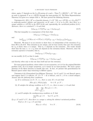
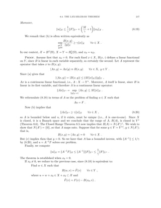
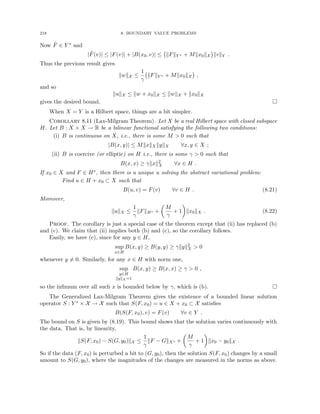
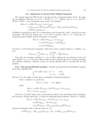
223. 8.5. APPLICATION TO SECOND ORDER ELLIPTIC EQUATIONS 223
In that case, for any α ∈ R,
B(u, v + α) = B(u, v) ,
so if we have a solution u ∈ H̃1(Ω), then also
F(v) = B(u, v) = B(u, v + α) = F(v + α) = F(v) + F(α)
implies that F(α) = 0 is required. That is, R ⊂ ker(F). This condition is called a compatibility
condition, and it says that the kernel of B(u, ·) is contained in the kernel of F; that is, f and g
must satisfy
hf, 1i(H1(Ω))∗,H1(Ω) − hg, 1iH−1/2(Ω),H1/2(Ω) = 0 ,
which is to say
Z
Ω
f(x) dx =
Z
∂Ω
g(x) dσ(x) ,
provided that f and g are integrable.
The compatibility condition arises from enlarging the space of test functions from H̃1(Ω) to
H1(Ω), which is necessary to prove that the solution to the variational problem also solves the
BVP. In abstract terms, we have the following situation. The problem is naturally posed for u
and v in a Hilbert space X. However, there is nonuniqueness because the set Y = {u ∈ X :
B(u, v) = 0 ∀v ∈ X} = {v ∈ X : B(u, v) = 0 ∀u ∈ X} is contained in the kernel of the natural
BC. But the problem is well behaved when posed over X/Y , which requires F|Y = 0, i.e., the
compatibility condition.
8.5.4. Elliptic regularity. We close this section with an important result from the theory
of elliptic PDE’s. See, e.g., [GT] or [Fo] for a proof. This result can be used to prove the
equivalence of the BVP and the variational problem in the case of Neumann BC’s.
Theorem 8.13 (Elliptic Regularity). Suppose that k ≥ 0 is an integer, Ω ⊂ Rd is a bounded
domain with a Ck+1,1(Ω)-boundary, a ∈ (Wk+1,∞(Ω))d×d is uniformly positive definite, b ∈
(Wk+1,∞(Ω))d, and c ∈ Wk,∞(Ω) is nonnegative. Suppose also that the bilinear form B :
H1(Ω) × H1(Ω) → R,
B(u, v) = (a∇u, ∇v)L2(Ω) + (bu, ∇v)L2(Ω) + (cu, v)L2(Ω) ,
is continuous and coercive on X, for X given below.
(a) If f ∈ Hk(Ω), uD ∈ Hk+2(Ω), and X = H1
0 (Ω), then the Dirichlet problem:
Find u ∈ H1
0 (Ω) + uD such that
B(u, v) = (f, v)L2(Ω) ∀v ∈ H1
0 (Ω) , (8.30)
has a unique solution u ∈ Hk+2(Ω) satisfying, for constant C 0 independent of f, u,
and uD,
kukHk+2(Ω) ≤ C kfkHk(Ω) + kuDkHk+3/2(∂Ω)
.
Moreover, k = −1 is allowed in this case, provided c ∈ W0,∞(Ω).
(b) If f ∈ Hk(Ω), g ∈ Hk+1/2(∂Ω), and X = H1(Ω), then the Neumann problem:
Find u ∈ H1(Ω) such that
B(u, v) = (f, v)L2(Ω) − (g, v)L2(∂Ω) ∀v ∈ H1
(Ω) , (8.31)

224. 224 8. BOUNDARY VALUE PROBLEMS
has a unique solution u ∈ Hk+2(Ω) satisfying, for constant C 0 independent of f, u,
and g,
kukHk+2(Ω) ≤ C kfkHk(Ω) + kgkHk+1/2(∂Ω)
.
Moreover, k = −1 is allowed if c ∈ C0,∞(Ω) and we intrepret kfkHk(Ω) as kfk(H1(Ω))∗ .
8.6. Galerkin Approximations
Often we wish to find some simple approximation to our BVP. This could be for computa-
tional purposes, to obtain an explicit approximation of the solution, or for theoretical purposes to
prove some property of the solution. We present here Galerkin methods, which give a framework
for such approximation.
Theorem 8.14. Suppose that H is a Hilbert space with closed subspaces
H0 ⊂ H1 ⊂ · · · ⊂ H
such that the closure of
∞
[
n=0
Hn is H. Suppose also that B : H ×H → R is a continuous, coercive
bilinear form on H and that F ∈ H∗. Then the variational problems, one for each n,
Find un ∈ Hn such that
B(un, vn) = F(vn) ∀vn ∈ Hn , (8.32)
have unique solutions. The same problem posed on H also has a unique solution u ∈ H, and
un → u in H .
Moreover, if M and γ are respectively the continuity and coercivity constants for B, then for
any n,
ku − unkH ≤
M
γ
inf
vn∈Hn
ku − vnkH . (8.33)
Furthermore, if B is symmetric, then for any n,
ku − unkB = inf
vn∈Hn
ku − vnkB , (8.34)
where k · kB = B(·, ·)1/2 is the energy norm.
Remark. Estimate (8.33) says that the approximation of u by un in Hn is quasi-optimal in
the H-norm; that is, up to the constant factor M/γ, un is the best approximation to u in Hn.
When B is symmetric, k·kB is indeed a norm, as the reader can verify, equivalent to the H-norm
by continuity and coercivity. Estimate (8.34) says that the Galerkin approximation un ∈ Hn is
optimal in the energy norm.
Proof. We have both
B(un, vn) = F(vn) ∀vn ∈ Hn ,
and
B(u, v) = F(v) ∀v ∈ H .
Existence of unique solutions is given by the Lax-Milgram Theorem. Since Hn ⊂ H, restrict
v = vn ∈ Hn in the latter and subtract to obtain that
B(u − un, vn) = 0 ∀vn ∈ Hn .

225. 8.6. GALERKIN APPROXIMATIONS 225
(We remark that in some cases B gives an inner-product, so in that case this relation says that
the error u−un is B-orthogonal to Hn; thus, this relation is referred to as Galerkin orthogonality.)
Replace vn by (u − un) − (u − vn) ∈ Hn for any vn ∈ Hn to obtain that
B(u − un, u − un) = B(u − un, u − vn) ∀vn ∈ Hn . (8.35)
Thus,
γku − unk2
H ≤ B(u − un, u − un) = B(u − un, u − vn) ≤ Mku − unkHku − vnkH ,
and (8.33) follows. If B is symmetric, then B is an inner-product, and the Cauchy-Schwarz
inequality applied to (8.35) gives
ku − unk2
B = B(u − un, u − un) = B(u − un, u − vn) ≤ ku − unkBku − vnkB ,
and (8.34) follows.
Finally, since
∞
[
n=0
Hn is dense in H, there are φn ∈ Hn such that φn → u in H as n → ∞.
Then
ku − unkH ≤
M
γ
inf
vn∈Hn
ku − vnkH ≤
M
γ
ku − φnkH ,
so un → u in H as n → ∞.
If (8.32) represents the equation for the critical point of an energy functional J : H → R,
then for any n,
inf
vn∈Hn
J(vn) = J(un) ≥ J(u) = inf
v∈H
J(v) .
That is, we find the function with minimal energy in the space Hn to approximate u. In this
minimization form, the method is called a Ritz method.
In the theory of finite element methods, one attempts to define explicitly the spaces Hn ⊂ H
in such a way that the equations (8.32) can be solved easily and so that the optimal error
inf
vn∈Hn
ku − vnkH
is quantifiably small. Such Galerkin finite element methods are extremely effective for computing
approximate solutions to elliptic BVP’s, and for many other types of equations as well. We now
present a simple example.
Example. Suppose that Ω = (0, 1) ⊂ R and f ∈ L2(0, 1). Consider the BVP
(
−u00
= f on (0, 1) ,
u(0) = u(1) = 0 .
(8.36)
The equivalent variational problem is:
Find u ∈ H1
0 (0, 1) such that
(u0
, v0
)L2 = (f, v)L2 ∀v ∈ H1
0 (0, 1) . (8.37)
We now construct a suitable finite element decomposition of H1
0 (0, 1). Let n ≥ 1 be an
integer, and define h = hn = 1/n and a grid xi = ih for i = 0, 1, ..., n of spacing h. Let
Hn = Hh = {v ∈ C0
(0, 1) : v(0) = v(1) = 0 and v(x) is a first degree
polynomial on [xi−1, xi] for i = 1, 2, ..., n} ;
that is, Hh consists of the continuous, piecewise linear functions. Note that Hh ⊂ H1
0 (0, 1), and
Hh is a finite dimensional vector space. We leave it to the reader to show that the closure of

226. 226 8. BOUNDARY VALUE PROBLEMS
∞
[
n=1
Hh is dense in H1
0 (0, 1). In fact, one can show that there is a constant C 0 such that for
any v ∈ H1
0 (0, 1) ∩ H2(0, 1),
min
vh∈Hh
kv − vhkH1 ≤ CkvkH2 h . (8.38)
The Galerkin finite element approximation is:
Find uh ∈ Hh such that
(u0
h, v0
h)L2 = (f, vh)L2 ∀vh ∈ Hh . (8.39)
If u solves (8.37), then Theorem 8.14 implies that
ku − uhkH1 ≤ C min
vh∈Hh
ku − vhkH1 ≤ CkukH2 h ≤ CkfkL2 h ,
using elliptic regularity. That is, the finite element approximations converge to the true solution
linearly in the grid spacing h.
The problem (8.39) is easily solved, e.g., by computer, since it reduces to a problem in linear
algebra. For each i = 1, 2, ..., n − 1, let φh,i ∈ Hh be such that
φh,i(xj) =
(
0 if i 6= j ,
1 if i = j .
Then {φh,i}n−1
i=1 forms a vector space basis for Hh, and so there are coefficients αi ∈ R such that
uh(x) =
n−1
X
j=1
αjφh,j(x) ,
and (8.39) reduces to
n−1
X
j=1
αj(φ0
h,j, φ0
h,i)L2 = (f, φh,i)L2 ∀i = 1, 2, ..., n − 1 ,
since it is sufficient to test against the basis functions φh,i. Let the (n − 1) × (n − 1) matrix M
be defined by
Mi,j = (φ0
h,j, φ0
h,i)L2
and the (n − 1)-vectors a and b by
aj = αj and bi = (f, φh,i)L2 .
Then our problem is simply Ma = b, and the coefficients of uh are given from the solution
a = M−1b (why is this matrix invertible?). In fact M is tridiagonal (i.e., all the nonzero entries
lie on the diagonal, subdiagonal, and superdiagonal), so the solution is easily and efficiently
computed.
8.7. Green’s Functions
Let L be a linear partial differential operator, such as is given in (8.3). Often we can find a
fundamental solution E ∈ D0 satisfying
LE = δ0 ,
wherein δ0 is the Dirac delta function or point mass at the origin. If for the moment we consider
that L has constant coefficients, then we know from the Malgrange and Ehrenpreis Theorem 5.28,

227. 8.7. GREEN’S FUNCTIONS 227
that such a fundamental solution exists. It is not unique, but for f ∈ D, say, the equation Lu = f
has a solution u = E ∗ f. However, u, defined this way, will generally fail to satisfy any imposed
boundary condition. To resolve this difficulty, we define a special fundamental solution in this
section. For maximum generality, we will often proceed formally, assuming sufficient smoothness
of all quantities involved to justify the calculations.
Let B denote a linear boundary condition operator (which generally involves the traces γ0
and/or γ1, and represents a Dirichlet, Neumann, or Robin boundary condition). For reasonable
f and g, we consider the BVP
Lu = f in Ω ,
Bu = g on ∂Ω .
(8.40)
Initially we will consider the homogeneous case where g = 0.
Definition. Suppose Ω ⊂ Rd, L is a linear partial differential operator, and B is a homo-
geneous linear boundary condition. We call G : Ω × Ω → R a Green’s function for L and B if,
for any f ∈ D, a weak solution u of (8.40) with g = 0 is given by
u(x) =
Z
Ω
G(x, y) f(y) dy . (8.41)
We assume here that ∂Ω is smooth enough to support the definition of the boundary condition.
Proposition 8.15. The Green’s function G(·, y) : Ω → R is a fundamental solution for L
with the point mass δy(·) = δ0(· − y): for a.e. y ∈ Ω,
LxG(x, y) = δ0(x − y) for x ∈ Ω
(wherein we indicate that L acts on the variable x by writing Lx instead). Moreover, G(x, y)
satisfies the homogeneous boundary condition
BxG(x, y) = 0 for x ∈ ∂Ω .
Proof. For any f ∈ D, we have u defined by (8.41), which solves Lu = f. We would like
to calculate
f(x) = Lu(x) = L
Z
Ω
G(x, y) f(y) dy =
Z
Ω
LxG(x, y) f(y) dy ,
which would indicate the result, but we need to justify moving L inside the integral. So for
φ ∈ D(Ω),
Z
Ω
f(x) φ(x) dx =
Z
Ω
Lu(x) φ(x) dx
=
Z
Ω
u(x) L∗
φ(x) dx
=
Z
Ω
Z
Ω
G(x, y) f(y) L∗
φ(x) dy dx
=
Z
Ω
Z
Ω
G(x, y) L∗
φ(x) f(y) dx dy
=
Z
Ω
hLxG(·, y), φi f(y) dy ,
showing that
hLxG(·, y), φi = φ(y) ,
that is, LxG(x, y) = δy(x).

228. 228 8. BOUNDARY VALUE PROBLEMS
That G(x, y) satisfies a homogeneous Dirichlet condition in x is clear. Other boundary
conditions involve normal derivatives, and it can be shown as above that G must satisfy them.
Remark. For a fundamental solution of a constant coefficient operator, LE = δ0, translation
implies that
LxE(x − y) = δy(x) ,
which can be understood as giving the response of the operator at x ∈ Rd, E(x − y), to a
point disturbance δy at y ∈ Rd. Multiplying by the weight f(y) and integrating (i.e., adding
the responses) gives the solution u = E ∗ f. When boundary conditions are imposed, a point
disturbance at y is not necessarily translation equivalent to a disturbance at ỹ 6= y. This is also
true of nonconstant coefficient operators. Thus the more general form of the Green’s function
being a function of two variables is required: G(x, y) is the response of the operator at x ∈ Ω to
a point disturbance at y ∈ Ω, subject also to the boundary conditions.
Given a fundamental solution E that is sufficiently smooth outside the origin, we can con-
struct the Green’s function by solving a related BVP. For almost every y ∈ Ω, solve
(
Lxwy(x) = 0 for x ∈ Ω ,
Bxwy(x) = BxE(x − y) for x ∈ ∂Ω ,
and then
G(x, y) = E(x − y) − wy(x)
is the Green’s function. Note that indeed LxG(x, y) = δ0(x − y) is a fundamental solution, and
that this one is special in that BxG(x, y) = 0 on ∂Ω.
It is generally difficult to find an explicit expression for the Green’s function, except in
special cases. However, its existence implies that the inverse operator of (L, B) is an integral
operator, and thus has many important properties, such as compactness. When G can be found
explicitly, it can be a powerful tool both theoretically and computationally.
We now consider the nonhomogeneous BVP (8.40). Suppose that there is u0 defined in Ω
such that Bu0 = g on ∂Ω. Then, if w = u − u0,
Lw = f − Lu0 in Ω ,
Bw = 0 on ∂Ω ,
(8.42)
and this problem has a Green’s function G(x, y). Thus our solution is
u(x) = w(x) + u0(x) =
Z
Ω
G(x, y) f(y) − Lu0(y)
dy + u0(x) .
This formula has limited utility, since we cannot easily find u0.
In some cases, the Green’s function can be used to define a different integral operator involv-
ing an integral on ∂Ω which involves g directly. To illustrate, consider (8.40) with L = −∆ + I,
where I is the identity operator. Now LxG(x, y) = δy(x), so this fact and integration by parts
implies that
u(y) =
Z
Ω
LxG(x, y) u(x) dx
=
Z
Ω
G(x, y) u(x) dx +
Z
Ω
∇xG(x, y) · ∇u(x) dx −
Z
∂Ω
∇xG(x, y) · ν u(x) dσ(x)
=
Z
Ω
G(x, y) Lu(x) dx +
Z
∂Ω
G(x, y)∇u(x) · ν dσ(x) −
Z
∂Ω
∇xG(x, y) · ν u(x) dσ(x) .

229. 8.8. EXERCISES 229
If B imposes the Dirichlet BC, so u = uD, then since Lu = f and G(x, y) itself satisfies the
homogeneous boundary conditions in x, we have simply
u(y) =
Z
Ω
G(x, y) f(x) dx −
Z
∂Ω
∇xG(x, y) · ν uD(x) dσ(x) .
This is called the Poisson integral formula. If instead B imposes the Neumann BC, so −∇u·ν = g,
then
u(y) =
Z
Ω
G(x, y) f(x) dx −
Z
∂Ω
G(x, y) g(x) dσ(x) .
Note that when g = 0, we have that
u(y) =
Z
Ω
G(x, y) f(y) dx =
Z
Ω
G(y, x) f(y) dx .
Since this formula holds for all f ∈ D, we conclude that G(x, y) = G(y, x), i.e., G is symmetric.
This is due to the fact that L is self adjoint in Ω. When L is not self-adjoint, we would need to
consider the Green’s function for the operator L∗, so that
u(y) =
Z
Ω
L∗
xG(x, y) u(x) dx =
Z
Ω
G(x, y) Lu(x) dx + boundary terms
=
Z
Ω
G(x, y) f(x) dx + boundary terms .
We remark that when a compatibility condition condition is required, it is not always possible
to obtain the Green’s function directly. For example, if L = −∆ and we have the nonhomoge-
neous Neumann problem, then
R
Ω δy(x) dx = 1 6= 0 as is required. So, instead we solve
(
−∆xG(x, y) = δy(x) − 1/|Ω| in Ω ,
−∇xG(x, y) · ν = 0 on ∂Ω ,
where |Ω| is the measure of Ω. Then our BVP (8.40) has the extra condition that the average
of u vanishes. Thus, as above,
u(y) = −
Z
Ω
∆xG(x, y) u(x) dx
=
Z
Ω
∇xG(x, y) · ∇u(x) dx −
Z
∂Ω
∇xG(x, y) · ν u(x) dσ(x)
= −
Z
Ω
G(x, y) ∆u(x) dx +
Z
∂Ω
G(x, y)∇u(x) · ν dσ(x)
=
Z
Ω
G(x, y) f(x) dx −
Z
∂Ω
G(x, y) g(x) dσ(x) .
8.8. Exercises
1. If A is a positive definite matrix, show that its eigenvalues are positive. Conversely, prove
that if A is symmetric and has positive eigenvalues, then A is positive definite.
2. Suppose that the hypotheses of the Generalized Lax-Milgram Theorem 8.10 are satisfied.
Suppose also that x0,1 and x0,2 are in X are such that the sets X + x0,1 = X + x0,2. Prove
that the solutions u1 ∈ X +x0,1 and u2 ∈ X +x0,2 of the abstract variational problem (8.18)
agree (i.e., u1 = u2). What does this result say about Dirichlet boundary value problems?

230. 230 8. BOUNDARY VALUE PROBLEMS
3. Suppose that we wish to find u ∈ H2(Ω) solving the nonlinear problem −∆u + cu2 = f ∈
L2(Ω), where Ω ⊂ Rd is a bounded Lipschitz domain. For consistency, we would require
that cu2 ∈ L2(Ω). Determine the smallest p such that if c ∈ Lp(Ω), you can be certain that
this is true, if indeed it is possible. The answer depends on d.
4. Suppose Ω ⊂ Rd is a connected Lipschitz domain and V ⊂ Ω has positive measure. Let
H = {u ∈ H1(Ω) : u|V = 0}.
(a) Why is H a Hilbert space?
(b) Prove the following Poincaré inequality: there is some C 0 such that
kukL2(Ω) ≤ Ck∇ukL2(Ω) ∀u ∈ H .
5. Suppose that Ω ⊂ Rd is a smooth, bounded, connected domain. Let
H =
u ∈ H2
(Ω) :
Z
Ω
u(x) dx = 0 and ∇u · ν = 0 on ∂Ω
.
Show that H is a Hilbert space, and prove that there exists C 0 such that for any u ∈ H,
kukH1(Ω) ≤ C
X
|α|=2
kDα
ukL2(Ω) .
6. Suppose Ω ⊂ Rd is a C1,1 domain. Consider the biharmonic BVP





∆2
u = f in Ω ,
∇u · ν = g on ∂Ω ,
u = uD on ∂Ω ,
wherein ∆2u = ∆∆u is the application of the Laplace operator twice.
(a) Determine appropriate Sobolev spaces within which the functions u, f, g, and uD should
lie, and formulate an appropriate variational problem for the BVP. Show that the two prob-
lems are equivalent.
(b) Show that there is a unique solution to the variational problem. [Hint: use the Elliptic
Regularity Theorem to prove coercivity of the bilinear form.]
(c) What would be the natural BC’s for this partial differential equation?
(d) For simplicity, let uD and g vanish and define the energy functional
J(v) =
Z
Ω
|∆v(x)|2
− 2f(x) v(x)
dx ,
Prove that minimization of J is equivalent to the variational problem.
7. Suppose Ω ⊂ Rd is a bounded Lipschitz domain. Consider the Stokes problem for vector u
and scalar p given by





−∆u + ∇p = f in Ω ,
∇ · u = 0 in Ω ,
u = 0 on ∂Ω ,
where the first equation holds for each coordinate (i.e., −∆uj + ∂p/∂xj = fj for each
j = 1, ..., d). This problem is not a minimization problem; rather, it is a saddle-point
problem, in that we minimize some energy subject to the constraint ∇ · u = 0. However, if

231. 8.8. EXERCISES 231
we work over the constrained space, we can handle this problem by the ideas of this chapter.
Let
H = {v ∈ (H1
0 (Ω))d
: ∇ · u = 0} .
(a) Verify that H is a Hilbert space.
(b) Determine an appropriate Sobolev space for f, and formulate an appropriate variational
problem for the constrained Stokes problem.
(c) Show that there is a unique solution to the variational problem.
8. Use the Lax-Milgram Theorem to show that, for f ∈ L2(Rd), there exists a unique solution
u ∈ H1(Rd) to the problem
−∆u + u = f in Rd
.
Be careful to justify integration by parts. [Hint: D is dense in H1(Rd).]
9. Consider the boundary value problem for u(x, y) : R2 → R such that
− uxx + ey
u = f , for (x, y) ∈ (0, 1)2
,
u(0, y) = 0, u(1, y) = cos(y) , for y ∈ (0, 1) .
Rewrite this as a variational problem and show that there exists a unique solution. Be sure
to define your function spaces carefully and identify where f must lie.
10. Let Ω ⊂ Rd be a bounded domain with a Lipschitz boundary, f ∈ L2(Ω), and α 0.
Consider the Robin boundary value problem



−∆u + u = f in Ω ,
∂u
∂ν
+ α u = 0 on ∂Ω .
(a) For this problem, formulate a variational principle
B(u, v) = (f, v) ∀v ∈ H1
(Ω) .
(b) Show that this problem has a unique weak solution.
11. Let Ω = [0, 1]d, define
H1
#(Ω) =
v ∈ H1
loc(Rd
) : v is periodic of period 1 in each direction and
Z
Ω
v dx = 0
,
and consider the problem of finding a periodic solution u ∈ H1
#(Ω) of
−∆u = f on Ω ,
where f ∈ L2(Ω).
(a) Define precisely what it means for v ∈ H1(Rd) to be periodic of period 1 in each direction.
(b) Show that H1
#(Ω) is a Hilbert space.
(c) Show that there is a unique solution to the partial differential equation.
12. Consider
B(u, v) = (a∇u, ∇v)L2(Ω) + (bu, ∇v)L2(Ω) + (cu, v)L2(Ω)
(a) Derive a condition on b to insure that B is coercive on H1(Ω) when a is uniformly positive
definite and c is uniformly positive.

232. 232 8. BOUNDARY VALUE PROBLEMS
(b) Suppose b = 0. If c 0, is B not coercive? Show that this is true on H1(Ω), but that
by restricting how negative c may be, B is still coercive on H1
0 (Ω).
13. Modify the statement of Theorem 8.14 to allow for nonhomogeneous essential boundary
conditions, and prove the result.
14. Let Ω ∈ Rd have a smooth boundary, Vn be the set of polynomials of degree up to n, for
n = 1, 2, ..., and f ∈ L2(Ω). Consider the problem: Find un ∈ Vn such that
(∇un, ∇vn)L2(Ω) + (un, vn)L2(Ω) = (f, vn)L2(Ω) for all vn ∈ Vn.
(a) Show that there exists a unique solution for any n, and that
kunkH1(Ω) ≤ kfkL2(Ω).
(b) Show that there is u ∈ H1(Ω) such that un
w
* u weakly in H1(Ω). Find a variational
problem satisfied by u. Justify your answer.
(c) Show that ku − unkH1(Ω) decreases monotonically to 0 as n → ∞.
(d) What can you say about u and ∇u · ν on ∂Ω?
15. Consider the finite element method in Section 8.6.
(a) Modify the method to account for nonhomogeneous Neumann conditions.
(b) Modify the method to account for nonhomogeneous Dirichlet conditions.
16. Compute explicitly the finite element solution to (8.36) using f(x) = x2(1 − x) and n = 4.
How does this approximation compare to the true solution?
17. Let Hh be the set of continuous piecewise linear functions defined on the grid xj = jh,
where h = 1/n for some integer n 0. Let the interpolation operator Ih : H1
0 (0, 1) → Hh
be defined by
Ihv(xj) = v(xj) ∀j = 1, 2, ..., n − 1 .
(a) Show that Ih is well defined, and that it is continuous. [Hint: use the Sobolev Imbedding
Theorem.]
(b) Show that there is a constant C 0 independent of h such that
kv − IhvkH1(xj−1,xj) ≤ CkvkH2(xj−1,xj)h .
[Hint: change variables so that the domain becomes (0, 1), where the result is trivial by
Poincaré’s inequality Corollary 7.18 and Theorem 8.12.]
(c) Show that (8.38) holds.
18. Consider the problem (8.36).
(a) Find the Green’s function.
(b) Instead impose Neumann BC’s, and find the Green’s function. [Hint: recall that now we
require −(∂2/∂x2)G(x, y) = δy(x) − 1.]

233. CHAPTER 9
Differential Calculus in Banach Spaces
and the Calculus of Variations
In this chapter, we move away from the rigid, albeit very useful confines of linear maps and
consider maps f : U → Y , not necessarily linear, where U is an open set in a Banach space X
and Y is also a Banach space.
As in finite-dimensional calculus, we begin the analysis of such functions by effecting a local
approximation. In one-variable calculus, we are used to writing
f(x) ∼
= f(x0) + f0
(x0)(x − x0) (9.1)
when f : R → R is continuously differentiable, say. This amounts to approximating f by an
affine function, a translation of a linear mapping. This procedure allows the method of linear
functional analysis to be brought to bear upon understanding a nonlinear function f.
9.1. Differentiation
In attempting to generalize the notion of a derivative to more than one dimension, one
realizes immediately that the one-variable calculus formula
f0
(x) = lim
h→0
f(x + h) − f(x)
h
(9.2)
cannot be taken over intact. First, the quantity 1/h has no meaning in higher dimensions.
Secondly, whatever f0(x) might be, it is plainly not going to be a number. Instead, just as in
multivariable calculus, it is a precise version of (9.1) that readily generalizes, and not (9.2). We
digress briefly for a definition.
Definition. Suppose X, Y are NLS’s and f : X → Y . If
kf(h)kY
khkX
→ 0 as h → 0 ,
we say that as h tends to 0, f is “little oh” of h, and we denote this as
kf(h)kY = o(khkX) .
Definition. Let f : U → Y where U ⊂ X is open and X and Y are normed linear spaces.
Let x ∈ U. We say that f is Fréchet differentiable (or strongly differentiable) at x if there is an
element A ∈ B(X, Y ) such that if
R(x, h) = f(x + h) − f(x) − Ah , (9.3)
then
1
khkX
kR(x, h)kY → 0 (9.4)
233

234. 234 9. DIFFERENTIAL CALCULUS IN BANACH SPACES AND THE CALCULUS OF VARIATIONS
as h → 0 in X, i.e.,
kR(x, h)kY = o(khkX) .
When it exists, we call A the Fréchet-derivative of f at x; it is denoted variously by
A = Ax = f0
(x) = Df(x) . (9.5)
Notice that this generalizes the one-dimensional idea of being differentiable. Indeed, if
f ∈ C1(R), then
R(x, h) = f(x + h) − f(x) − f0
(x)h =
f(x + h) − f(x)
h
− f0
(x)
h ,
and so
|R(x, h)|
|h|
=
f(x + h) − f(x)
h
− f0
(x) → 0
as h → 0 in R. Note that B(R, R) = R, and thus that the product f0(x)h may be viewed as the
linear mapping that sends h to f0(x)h.
We can also think of Df as a mapping of X × X into Y via the correspondence
(x, h) 7−→ f0
(x)h .
Proposition 9.1. If f is Fréchet differentiable, then Df(x) is unique and f is continuous
at x. Moreover, if g is Fréchet differentiable and α, β ∈ F, then
D(αf + βg)(x) = αDf(x) + βDg(x) .
Proof. Suppose A, B ∈ B(X, Y ) are such that
f(x + h) − f(x) − Ah = RA(x, h)
and
f(x + h) − f(x) − Bh = RB(x, h) ,
where
kRA(x, h)kY
khkX
→ 0 and
kRB(x, h)kY
khkX
→ 0
as h → 0 in X. It follows that
kA − BkB(X,Y ) =
1
ε
sup
khkX =ε
kAh − BhkY
= sup
khkX =ε
kRB(x, h) − RA(x, h)kY
khkX
≤ sup
khkX =ε
kRB(x, h)kY
khkX
+ sup
khkX =ε
kRA(x, h)kY
khkX
,
and the right-hand side may be made as small as we like by taking ε small enough. Thus A = B.
Continuity of f at x is straightforward since
kf(x + h) − f(x)kY = kDf(x)h + R(x, h)kY
≤ kDf(x)kB(X,Y )khkY + kR(x, h)kY ,
and the right-hand side tends to 0 as h → 0 in X.
The final result is left as an exercise.

235. 9.1. DIFFERENTIATION 235
In fact, we have much more than mere continuity. The following result is often useful. It
says that when f is differentiable, it is locally Lipschitz.
Lemma 9.2 (Local-Lipschitz property). If f : U → Y is differentiable at x ∈ U, then given
ε 0, there is a δ = δ(x, ε) 0 such that for all h with khkX ≤ δ,
kf(x + h) − f(x)kY ≤
kDf(x)kB(X,Y ) + ε
khkX . (9.6)
Proof. Simply write
f(x + h) − f(x) = R(x, h) + Df(x)h . (9.7)
Since f is differentiable at x, given ε 0, there is a δ 0 such that khkX ≤ δ implies
kR(x, h)kY
khkX
≤ ε .
Then (9.7) implies the advertised results.
Examples. 1. If f(x) = Ax, where A ∈ B(X, Y ), then f(x+h)−f(x) = Ah, so f is Fréchet
differentiable everywhere and
Df(x) = A
for all x ∈ X.
2. Let X = H be a Hilbert-space over R. Let f(x) = (x, Ax)H where A ∈ B(H, H). Then,
f : H → R and
f(x + h) − f(x) = (x, Ah)H + (h, Ax)H + (h, Ah)H
=
(A∗
+ A)x, h
H
+ (h, Ah)H .
Hence if we define, for x, h ∈ X,
Df(x)h =
(A∗
+ A)x, h
H
,
then
kf(x + h) − f(x) − Df(x)hkY ≤ khk2
XkAkB(X,Y ) .
Thus Df(x) ∈ H∗ = B(H, R) is the Riesz-map associated with the element (A∗ + A)x.
3. Let f : Rn → R and suppose f ∈ C1(Rn), which is to say ∂if exists and is continuous on
Rn, 1 ≤ i ≤ n. Then Df(x) ∈ B(Rn, R) is defined by
Df(x)h = ∇f(x) · h .
4. Let f : Rn → Rm and suppose f ∈ C1(Rn, Rm), which is to say each of the component
functions f = (f1, . . . , fm) as a R-valued function, having all its first partial derivatives, and
each of these is continuous. Then f is Fréchet differentiable and
Df(x)h = [∂jfi(x)]h ,
where the latter is matrix multiplication and the matrix itself is the usual Jacobian matrix.
That is, Df(x) ∈ B(Rn, Rm) is an m × n matrix, and the ith component of Df(x)h is
n
X
j=1
∂jfi(x)hj .

236. 236 9. DIFFERENTIAL CALCULUS IN BANACH SPACES AND THE CALCULUS OF VARIATIONS
5. Let ϕ ∈ Lp(Rd), where p ≥ 1, p an integer, and define
f(ϕ) =
Z
Rd
ϕp
(x) dx .
Then f : Lp(Rd) → R, f is Fréchet differentiable and
Df(ϕ)h = p
Z
Rd
ϕp−1
(x)h(x) dx .
To see this, we use the Binomial Theorem:
f(ϕ + h) − f(ϕ) =
Z
Rd
[(ϕ + h)p
(x) − ϕp
(x)] dx
=
Z
Rd
ϕp
(x) + pϕp−1
(x)h(x) +
p
2
ϕp−2
(x)h2
(x) + ... + hp
(x) − ϕp
(x)
dx
= p
Z
Rd
ϕp−1
(x) h(x) dx +
Z
Rd
p
2
ϕp−2
(x) h2
(x) + ... + hp
(x)
dx .
There is a differentiability notion weaker than Fréchet differentiable, but still occasionally
useful. In this conception, we only ask the function f to be differentiable in a specified direction.
Let h ∈ X and consider the Y -valued function of the real variable t:
g(t) = f(x + th) .
Definition. Suppose f : X → Y . Then f is Gateaux differentiable (or weakly differentiable)
at x ∈ X in the direction h ∈ X if there is an A ∈ B(X, Y ) such that
1
t
kf(x + th) − f(x) − tAhk → 0
as t → 0. The Gateaux-derivative is denoted by
A = Dhf(x) .
Moreover, f is Gateaux differentiable at x if it is Gateaux differentiable at x in every direction
h ∈ X.
Proposition 9.3. If f is Fréchet differentiable, then it is Gateaux differentiable.
Remark. The converse is not valid. The function f : R2 → R given by
f(x) =
(
0 , if x2 = 0 ,
x3
1/x2 , if x2 6= 0 ,
is not continuous at the origin. For instance f((t, t3)) → 1 as t → 0, but f(0) = 0. However, f
is Gateaux differentiable at (0, 0) in every direction h since
f(th) − f(0)
t
=
f(th)
t
=
(
0 if h2 = 0 ,
t(h3
1/h2) if h2 6= 0 .
The limit as t → 0 exists and is zero, whatever the value of h.
Theorem 9.4 (Chain Rule). Let X, Y, Z be NLS’s and U ⊂ X open, V ⊂ Y open, f : U → Y
and g : V → Z. Let x ∈ U and y = f(x) ∈ V . Suppose g is Fréchet differentiable at y and
f is Gateaux- (respectively, Fréchet-) differentiable at x. Then g ◦ f is Gateaux- (respectively,
Fréchet-) differentiable at x and
D(g ◦ f)(x) = Dg(y) ◦ Df(x) .

237. 9.1. DIFFERENTIATION 237
X
x
h x + h
s
*
-
f
Y
u
y = f(x)
f(x + h)
s
A
A
K
-
g
Z
z = g(f(x))
g(f(x + h))
s
Figure 1. The Chain Rule.
Proof. The proof is given for the case where both maps are Fréchet differentiable. The
proof for the Gateaux case is similar. Write
Rf (x, h) = f(x + h) − f(x) − Df(x)h
and
Rg(y, k) = g(y + k) − g(y) − Dg(y)k .
By assumption,
Rf (x, h)
khk
Y
−
→ 0 as h
X
−
→ 0 (9.8)
and
Rg(y, k)
kkk
Z
−
→ 0 as k
Y
−
→ 0 . (9.9)
Define
u = u(h) = f(x + h) − f(x) = f(x + h) − y . (9.10)
By continuity, u(h) → 0 as h → 0. Now consider the difference
g(f(x + h)) − g(f(x)) = g(f(x + h)) − g(y)
= Dg(y)[f(x + h) − y] + Rg(y, u)
= Dg(y)[Df(x)h + Rf (x, h)] + Rg(y, u)
= Dg(y)Df(x)h + R(x, h) ,
where
R(x, h) = Dg(y)Rf (x, h) + Rg(y, u) .
We must show that R(x, h) = o(khkX) as h → 0. Notice that
kDg(y)Rf (x, h)kZ
khkX
≤ kDg(y)kB(Y,Z)
kRf (x, h)kY
khkX
→ 0 as h → 0
because of (9.8). The second term is slightly more interesting. We are trying to show
kRg(y, u)kZ
khkX
→ 0 (9.11)
as h → 0. This does not follow immediately from (9.9). However, the local-Lipschitz property
comes to our rescue.

238. 238 9. DIFFERENTIAL CALCULUS IN BANACH SPACES AND THE CALCULUS OF VARIATIONS
If u = 0, then Rg(y, u) = 0. If not, then multiply and divide by kukY to reach
kRg(y, u)kZ
khkX
=
kRg(y, u)k
kukY
kukY
khkX
. (9.12)
Let ε 0 be given and suppose without loss of generality that ε ≤ 1. There is a σ 0 such
that if kkkY ≤ σ, then
kRg(y, k)kZ
kkkY
≤ ε . (9.13)
On the other hand, because of (9.6), there is a δ 0 such that khkX ≤ δ implies
ku(h)kY = kf(x + h) − f(x)kY ≤
kDf(x)kB(X,Y ) + 1
khkX ≤ σ (9.14)
(simply choose δ so that δ(kDf(x)kB(X,Y ) + 1) ≤ σ in addition to it satisfying the smallness
requirement in Lemma 9.2). With this choice of δ, if khkX ≤ δ, then (9.12) implies
kRg(y, u)kZ
khkX
≤ ε
kDf(x)kB(X,Y ) + 1
.
The result follows.
Proposition 9.5 (Mean-Value Theorem for Curves). Let Y be a NLS and ϕ : [a, b] → Y be
continuous, where a b are real numbers. Suppose ϕ0(t) exists on (a, b) and that kϕ0(t)kB(R,Y ) ≤
M. Then
kϕ(b) − ϕ(a)kY ≤ M(b − a) . (9.15)
Remark. Every bounded linear operator from R to Y is given by t 7→ ty for some fixed
y ∈ Y . Hence we may identify ϕ0(t) with this element y. Notice in this case that y can be
obtained by the elementary limit
y = ϕ0
(t) = lim
s→0
ϕ(t + s) − ϕ(t)
s
.
Proof. Fix an ε 0 and suppose ε ≤ 1. For any t ∈ (a, b), there is a δt = δ(t, ε) such that
if |s − t| δt, s ∈ (a, b), then
kϕ(s) − ϕ(t)kY (M + ε)|s − t| (9.16)
by the Local-Lipschitz Lemma 9.2. Let
S(t) = Bδt (t) ∩ (a, b) ,
which is open. Then if a ã b̃ b,
[ã, b̃] ⊂
[
t∈[ã,b̃]
S(t) .
Hence by compactness, there is a finite sub-cover, of, say, N intervals, S(ã), S(t2), S(t4), . . . , S(b̃),
where
ã = t0 t2 · · · t2N = b̃ ,
such that also S(t2k+2) ∩ S(t2k) 6= ∅ for all k. Choose points t2k+1 ∈ S(t2k+2) ∩ S(t2k), enrich
the partition to
ã = t0 t1 t2 · · · t2N = b̃ ,

239. 9.1. DIFFERENTIATION 239
and note that
kϕ(tk+1) − ϕ(tk)kY ≤ (M + ε)|tk+1 − tk|
for all k. Hence
kϕ(b̃) − ϕ(ã)kY ≤
2N
X
k=1
kϕ(tk) − ϕ(tk−1)kY
≤ (M + ε)
2N
X
k=1
(tk − tk−1) = (M + ε)(b̃ − ã) .
By continuity, we may take the limit on b̃ → b and ã → a, and the same inequality holds. Since
ε 0 was arbitrary, (9.15) follows.
Remark. The Mean-Value Theorem for curves can be used to give reasonable conditions
under which Gateaux differentiability implies Fréchet differentiability. Here is another corollary
of this result.
Theorem 9.6 (Mean-Value Theorem). Let X, Y be NLS’s and U ⊂ X open. Let f : U → Y
be Fréchet differentiable everywhere in U and suppose the line segment
` = {tx2 + (1 − t)x1 : 0 ≤ t ≤ 1}
is contained in U. Then
kf(x2) − f(x1)kY ≤ sup
x∈`
kDf(x)kB(X,Y )kx2 − x1kX . (9.17)
Proof. Define ϕ : [0, 1] → Y by
ϕ(t) = f((1 − t)x1 + tx2) = f(x1 + t(x2 − x1)) = f(γ(t)) ,
where γ : [0, 1] → X. Certainly ϕ is differentiable on [0, 1] by the chain rule. By Proposition 9.5,
kf(x2) − f(x1)kY = kϕ(1) − ϕ(0)kY ≤ sup
0≤t≤1
kϕ0
(t)kY .
but, the chain rule insures that
ϕ0
(t) = Df(γ(t)) ◦ γ0
(t) = Df(γ(t))(x2 − x1) ,
so
kϕ0
(t)kY ≤ kDf(γ(t))kB(X,Y )kx2 − x1kX
≤ sup
x∈`
kDf(x)kB(X,Y )kx2 − x1kX .
One can generalize the discussion immediately to partial Fréchet differentiability. Suppose
X1, . . . , Xm are NLS’s over F and Y another NLS. Let
X = X1 ⊕ · · · ⊕ Xm
be a direct sum of the Xi’s. Thus, as a point set, X = X1 × · · · × Xm is the Cartesian product,
and the vector-space operations are carried out componentwise. Let the norm be any of the
equivalent functions
kxkX =
m
X
j=1
kxikp
Xi
1/p
= (kx1kX1 , · · · , kxmkXm ) `p
, (9.18)

240. 240 9. DIFFERENTIAL CALCULUS IN BANACH SPACES AND THE CALCULUS OF VARIATIONS
where p ∈ [1, ∞] (modified in the usual way if p = ∞) and x = (x1, . . . , xm), which makes X into
a NLS. It is a Banach space if and only if Xi is a Banach space, 1 ≤ i ≤ m. Conversely, given
a Banach space X, we could decompose it into a direct sum of subspaces Y = X1 ⊕ · · · ⊕ Xm,
with norms k · kXi = k · kX, so that X and Y would be equivalent Banach spaces.
Definition. Let X = X1 ⊕ · · · ⊕ Xm as above. Let U ⊂ X be open and F : U → Y , Y a
NLS. Let x = (x1, . . . , xm) ∈ U and fix an integer k ∈ [1, m]. For z near xk in Xk, the point
(x1, . . . , xk−1, z, xk+1, . . . , xm) lies in U, since U is open. Define
fk(z) = F(x1, . . . , xk−1, z, xk+1, . . . , xm) .
Then fk maps an open subset of Xk into Y . If fk has a Fréchet derivative at z = xk, then we
say F has a kth-partial derivative at x and define
DkF(x) = Dfk(xk) .
Notice that DkF(x) ∈ B(Xk, Y ).
Proposition 9.7. Let X = X1 ⊕ · · · ⊕ Xm be the direct sum of NLS’s, U ⊂ X open, and
F : U → Y , another NLS. Suppose DjF(x) exists for x ∈ U and 1 ≤ j ≤ m, and that these
linear maps are continuous as a function of x at x0 ∈ U. Then F is Fréchet differentiable at x0
and for h = (h1, . . . , hm) ∈ X,
DF(x0)h =
m
X
j=1
DjF(x0)hj . (9.19)
Proof. The right-hand side of (9.19) defines a bounded linear map on X. Indeed, it may
be written as
Ah =
m
X
j=1
DjF(x0) ◦ Πjh
where Πj : X → Xj is the projection on the jth-component. So A is a sum of compositions of
bounded operators and so is itself a bounded operator. Define
R(h) = F(x0 + h) − F(x0) − Ah .
It suffices to show that R : X → Y is such that
R(h)
khkX
→ 0
as h → 0. Let ε 0 be given. Because F is partially Fréchet differentiable and A is linear, it
follows immediately from the chain rule that R is partially Fréchet differentiable in h and
DjR(h) = DjF(x0 + h) − DjF(x0) .
Since the partial Fréchet-derivatives are continuous as a function of x at x0 it follows there is a
δ 0 such that if kh0kX ≤ δ, then
kDjR(h0
)kB(Xj,Y ) ≤ ε for 1 ≤ j ≤ m . (9.20)
On the other hand,
kR(h0
)kY ≤ kR(h0
) − R(0, h0
2, . . . , h0
m)kY + kR(0, h0
2, . . . , h0
m) − R(0, 0, h0
3, . . . , h0
m)kY
+ · · · + kR(0, . . . , 0, h0
m) − R(0, . . . , 0)kY .
(9.21)

241. 9.2. FIXED POINTS AND CONTRACTIVE MAPS 241
Thus, if khkX ≤ δ, then by the Mean-Value Theorem applied to the mappings
Rj(hj) = R(0, . . . , 0, hj, h0
j+1, . . . , h0
m) ,
it is determined on the basis of (9.20) that
kRj(hj) − Rj(0)kY ≤ sup
t∈[0,1]
kDRj(thj)kB(Xj,Y )khjkXj
= sup
t∈[0,1]
kDjR(0, . . . , 0, thj, h0
j+1, . . . , h0
m)kB(Xj,Y )khjkXj
≤ εkhjkXj , for 1 ≤ j ≤ m .
Choosing in (9.18) the `1-norm on X, it follows from (9.21) and the last inequalities that for
kh0kX δ,
kR(h0
)kY ≤ ε
m
X
j=1
khjkXj = εkhkX .
(If another `p-norm is used in (9.18), we merely get a fixed constant multiple of the right-hand
side above.) The result follows.
9.2. Fixed Points and Contractive Maps
Definition. Let (X, d) be a metric space and G : X → X. The mapping G is a contraction
if there is a θ with 0 ≤ θ 1 such that
d(G(x), G(y)) ≤ θd(x, y) for all x, y ∈ X .
A fixed point of the mapping G is an x ∈ X such that x = G(x).
A contraction map is a Lipschitz map with Lipschitz constant less than 1. Such maps are
also continuous.
Theorem 9.8 (Banach Contraction-Mapping Principle). Let (X, d) be a complete metric
space and G a contraction mapping of X. Then there is a unique fixed point of G in X.
Proof. If there were two fixed points x and y, then
d(x, y) = d(G(x), G(y)) ≤ θd(x, y) ,
and since d(x, y) ≥ 0 and 0 ≤ θ 1, it follows that d(x, y) = 0, whence x = y.
For existence of a fixed point, argue as follows. Fix an x0 ∈ X and let x1 = G(x0), x2 = G(x1)
and so on. We claim the sequence {xn}∞
n=0 of iterates is a Cauchy sequence.
If this {xn}∞
n=0 is Cauchy, then since (X, d) is complete, there is an x̄ such that xn → x̄.
But then G(xn) → G(x̄) by continuity. Since G(xn) = xn+1, it follows that G(x̄) = x̄.
To see {xn}∞
n=0 is a Cauchy sequence, first notice that
d(x1, x2) = d(G(x0), G(x1)) ≤ θd(x0, x1) .
Continuing in this manner,
d(xn, xn+1) = d(G(xn−1), G(xn)) ≤ θd(xn−1, xn)
for n = 1, 2, 3, . . . . In consequence, we derive by induction that
d(xn, xn+1) ≤ θn
d(x0, x1) , for n = 0, 1, 2, . . . .

242. 242 9. DIFFERENTIAL CALCULUS IN BANACH SPACES AND THE CALCULUS OF VARIATIONS
Thus, if n ≥ 0 is fixed and m n, then
d(xn, xm) ≤ d(xn, xn+1) + d(xn+1, xn+2) + · · · + d(xm−1, xm)
≤ (θn
+ · · · + θm−1
)d(x0, x1)
= θn
(1 + · · · + θm−n−1
)d(x0, x1)
= θn 1 − θm−n
1 − θ
d(x0, x1)
≤
θn
1 − θ
d(x0, x1) .
As θ 1, the right-hand side of the last inequality can be made as small as desired, independently
of m, by taking n large enough.
Not only does this result provide existence and uniqueness, but the proof is constructive.
Indeed, the proof consists of generating a sequence of approximations to x = G(x).
Corollary 9.9 (Fixed Point Iteration). Suppose that (X, d) be a complete metric space, G
a contraction mapping of X with contraction constant θ, and x0 ∈ X. If the sequence {xn}∞
n=0
is defined successively by xn+1 = G(xn) for n = 0, 1, 2, ..., then xn → x, where x is the unique
fixed point of G in X. Moreover,
d(xn, x) ≤
θn
1 − θ
d(x0, x1) .
Example. Consider the initial value prooblem (IVP)
ut = cos(u(t)) , t 0 ,
u(0) = u0 .
We would like to obtain a solution to the problem, at least up to some final time T 0, using
the fixed point theorem. At the outset we require two things: a complete metric space within
which to seek a solution, and a map on that space for which a fixed point is the solution to our
problem. It is not easy to handle the differential operator directly in this context, so we remove
it through integration:
u(t) = u0 +
Z t
0
cos(u(s)) ds .
Now it is natural to seek a continuous function as a solution, say in X = C0([0, T]), for some as
yet unknown T 0. It is also natural to consider the function
G(u) = u0 +
Z t
0
cos(u(s)) ds ,
which clearly takes X to X and has a fixed point at the solution to our IVP. To see if G is
contractive, consider two functions u and v in X and compute
kG(u) − G(v)kL∞ = sup
0≤t≤T
Z t
0
cos(u(s)) − cos(v(s))
ds
= sup
0≤t≤T
Z t
0
(− sin(w(s))(u(s) − v(s)) ds
≤ Tku − vkL∞ ,

243. 9.2. FIXED POINTS AND CONTRACTIVE MAPS 243
wherein we have used the ordinary mean value theorem for functions of a real variable. So, if
we take T = 1/2, we have a unique solution by the Banach Contraction Mapping Theorem.
Since T is a fixed number independent of the solution u, we can iterate this process, starting at
t = 1/2 (with “initial condition” u(1/2)) to extend the solution uniquely to t = 1, and so on, to
obtain a solution for all time.
Example. Let κ ∈ L1(R), ϕ ∈ CB(R) and consider the nonlinear operator
Φu(x, t) = ϕ(x) +
Z t
0
Z ∞
−∞
κ(x − y)(u(y, s) + u2
(y, s)) dy ds .
We claim that there exists T = T(kϕk∞) 0 such that Φ has a fixed point in the space
X = CB(R × [0, T]).
Since κ is in L1(R), Φu makes sense. If u ∈ CB(R), then it is an easy exercise to see Φu ∈ X.
Indeed, Φu is C1 in the temporal variable and continuous in x by the Dominated Convergence
Theorem. That is, Φ : X → X; however, Φ is not contractive on all of X.
Let R 0 and BR the closed ball of radius R about 0 in X. We want to show if R and T
are chosen well, Φ : BR → BR is a contraction. Let u, v ∈ BR and consider
kΦu − ΦvkX = sup
(x,t)∈R×[0,T]
Z t
0
Z ∞
−∞
κ(x − y)(u − v + u2
− v2
) dy ds
≤ T sup
(x,t)∈R×[0,T]
Z ∞
−∞
|κ(x − y)(u − v + u2
− v2
)| dy
≤ TkκkL1
ku − vkX + ku2
− v2
kX
≤ TkκkL1
1 + kukX + kvkX
ku − vkX
≤ TkκkL1 (1 + 2R)ku − vkX .
Let
θ = T(1 + 2R)kκkL1 ,
choose R = 2kϕkL∞ and then choose T so that θ = 1/2. With these choices, Φ is contractive on
BR and if u ∈ BR, then indeed
kΦukX ≤ kΦu − Φ0kX + kΦ0kX
≤ θku − 0kX + kϕkL∞
≤
1
2
R +
1
2
R = R .
That is, Φ : BR → BR, Φ is contractive, and BR, being closed, is a complete metric space. We
conclude that there exists a unique u ∈ BR such that
u = Φu .
Why do we care? Consider
∂u
∂t
+
∂u
∂x
+ 2u
∂u
∂x
−
∂3u
∂x2∂t
= 0 , (9.22)

244. 244 9. DIFFERENTIAL CALCULUS IN BANACH SPACES AND THE CALCULUS OF VARIATIONS
a nonlinear, dispersive wave equation. Write it as
(1 − ∂2
x)ut = −ux − 2uux ≡ f .
The left-hand side is a nice operator, at least from the point of view of the Fourier Transform,
as we will see in a moment, while the terms defining f are more troublesome. Take the Fourier
transform on x to reach
(1 + ξ2
)ût = ˆ
f , i.e., ût =
1
1 + ξ2
ˆ
f ,
whence, by taking the inverse Fourier transform, it is formally deduced that
ut = κ̃ ∗ f = −κ̃ ∗ (ux + 2uux) = −κ̃ ∗ (u + u2
)x
where
κ̃(x) =
√
2πF−1
1
1 + ξ2
=
1
2
e−|x|
.
Let κ = −κ̃x ∈ L1(R) to conclude
ut(x, t) = κ ∗ (u + u2
) .
Now integrate over [0, t] and use the Fundamental Theorem of Calculus with constant of inte-
gration u(x, 0) = ϕ(x) ∈ CB(R) to reach
u(x, t) = ϕ(x) +
Z t
0
κ ∗ (u + u2
) ds ,
which has the form with which we started the example. Thus our fixed point Φu = u is formally
a solution to (9.22), at least up to the time T, with the initial condition u(x, 0) = ϕ(x).
Corollary 9.10. Let X be a Banach space and f : X → X a differentiable mapping.
Suppose kDf(x)kB(X,X) ≤ κ 1 for x ∈ BR(0). If there is an x0 ∈ BR(0) such that Br(x0) ⊂
BR(0) for some r ≥ kf(x0) − x0k/(1 − κ), then f has a unique fixed point in Br(x0).
That is, a map f which is locally contractive and for which we can find a point not moved
too far by f has a fixed point, and the iteration
x0, x1 = f(x0), x2 = f(x1), · · · ,
generates a sequence that converges to a fixed point.
Proof. In fact, we show that f is a contraction mapping of Br(x0). First, by the Mean-
Value Theorem, for any x, y ∈ BR(0),
kf(x) − f(y)k ≤ κkx − yk .
Hence f is contractive. The Contraction-Mapping Theorem will apply as soon as we know that
f maps Br(x0) into itself, since Br(x0) is a complete metric space. By the triangle inequality, if
x ∈ Br(x0),
kf(x) − x0k ≤ kf(x) − f(x0)k + kf(x0) − x0k
≤ κkx − x0k + (1 − κ)r ≤ r .

245. 9.3. NONLINEAR EQUATIONS 245
9.3. Nonlinear Equations
Developed here are some helpful techniques for understanding when a nonlinear equation has
a solution. The basic tool is to convert the equation into a fixed point problem. For example,
when X, Y are Banach spaces and f : X → Y , the problem of finding x for fixed y in
f(x) = y
is equivalent to finding a fixed point of
G(x) = x − Tx(f(x) − y) ,
where Tx : Y → X vanishes only at 0. If Tx = T is independent of x, we have that
DG(x) = I − T ◦ Df(x) ,
so G is a contraction provided T can be chosen to make kI − T ◦ Df(x)k 1.
Theorem 9.11 (Simplified Newton Method). Let X, Y be Banach spaces and f : X → Y a
differentiable mapping. Suppose A = Df(x0) has a bounded inverse and that
kI − A−1
Df(x)k ≤ κ 1 (9.23)
for all x ∈ Br(x0), for some r 0. Let
δ =
(1 − κ)r
kA−1kB(Y,X)
.
Then the equation
f(x) = y
has a unique solution x ∈ Br(x0) whenever y ∈ Bδ(f(x0)).
Proof. Let y ∈ Bδ(f(x0)) be given and define a mapping gy : X → X by
gy(x) = x − A−1
(f(x) − y) . (9.24)
Notice that gy(x) = x if and only if f(x) = y. Note also that
Dgy(x) = I − A−1
Df(x) ,
by the chain rule. By assumption, kDgy(x)kB(X,X) ≤ κ 1 for x ∈ Br(x0), so gy is a contraction
on Br(x0) by continuity. Moreover, by the choice of y and δ, for x ∈ Br(x0),
kgy(x) − x0kX ≤ kgy(x) − gy(x0)kX + kgy(x0) − x0kX
≤ r + kA−1
(f(x0) − y)kX r + (1 − κ)r = r .
The hypotheses of Theorem 9.8 are verified, i.e., gy is a contractive map of Br(x0), and the
conclusion follows.
Remark. If Df(x) is continuous as a function of x, then Hypothesis (9.23) is true for
r small enough. Thus another conclusion is that at any point x where Df(x) is boundedly
invertible, there is an r 0 and a δ 0 such that f(Br(x)) ⊃ Bδ(f(x)) and f is one-to-one on
Br(x) ∩ f−1(Bδ(f(x))).

246. 246 9. DIFFERENTIAL CALCULUS IN BANACH SPACES AND THE CALCULUS OF VARIATIONS
Notice the algorithm that is implied by the proof. Given y, start with a guess x0 and form
the sequence
xn+1 = gy(xn) = xn − A−1
(f(xn) − y) .
If things are as in the theorem, the sequence converges to the solution of f(x) = y in Br(x0).
Notice that if x is the solution, then
kxn − xkX = kgy(xn−1) − gy(x)kX
≤ κkxn−1 − xkX
≤ · · ·
≤ κn
kx0 − xkX .
More can be shown. We leave the rather lengthy proof of the following result to the reader.
Theorem 9.12 (Newton-Kantorovich Method). Let X, Y be Banach spaces and f : X → Y
a differentiable mapping. Assume that there is an x0 ∈ X and an r 0 such that
(i) A = Df(x0) has a bounded inverse, and
(ii) kDf(x1) − Df(x2)kB(X,Y ) ≤ κkx1 − x2k
for all x1, x2 ∈ Br(x0). Let y ∈ Y and set
ε = kA−1
(f(x0) − y)kX .
For any y such that
ε ≤
r
2
and 4εκkA−1
kB(Y,X) ≤ 1 ,
the equation
y = f(x)
has a unique solution in Br(x0). Moreover, the solution is obtained as the limit of the Newton-
iterates
xk+1 = xk − Df(xk)−1
(f(xk) − y)
starting at x0. The convergence is asymptotically quadratic; that is,
kxk+1 − xkkX ≤ Ckxk − xk−1k2
X ,
for k large, where C does not depend on k.
Theorem 9.13 (Inverse Function Theorem I). Suppose the hypotheses of the Simplified New-
ton Method hold. Then the inverse mapping f−1 : Bδ(f(x0)) → Br(x0) is Lipschitz.
Proof. Let y1, y2 ∈ Bδ(f(x0)) and let x1, x2 be the unique points in Br(x0) such that
f(xi) = yi, for i = 1, 2. Fix a y ∈ Bδ(f(x0)), y = y0 = f(x0) for example, and reconsider the
mapping gy defined in (9.24). As shown, gy is a contraction mapping of Br(x0) into itself with
Lipschitz constant κ 1. Then
kf−1
(y1) − f−1
(y2)kX = kx1 − x2kX
= kgy(x1) − gy(x2) + A−1
(f(x2) − f(x1))kX
≤ κkx1 − x2kX + kA−1
kB(Y,X)ky2 − y1kY .
It follows that
kx1 − x2k ≤
kA−1kB(Y,X)
1 − κ
ky1 − y2k

247. 9.3. NONLINEAR EQUATIONS 247
and hence that f−1 is Lipschitz with constant at most kA−1kB(Y,X)/(1 − κ).
Earlier, we agreed that two Banach spaces X and Y are isomorphic if there is a T ∈ B(X, Y )
which is one-to-one and onto (and hence with bounded inverse by the Open Mapping Theorem).
Isomorphic Banach spaces are indistinguishable as Banach spaces. A local version of this idea
is now introduced.
Definition. Let X, Y be Banach spaces and U ⊂ X, V ⊂ Y open sets. Let f : U → V
be one-to-one and onto. Then f is called a diffeomorphism on U and U is diffeomorphic to V
if both f and f−1 are C1, which is to say f and f−1 are Fréchet differentiable throughout U
and V , respectively, and their derivatives are continuous on U and V , respectively. That is, the
maps
x 7−→ Df(x) and y 7−→ Df−1
(y)
are continuous from U to B(X, Y ) and V to B(Y, X), respectively.
Note that a diffeomorphism is stronger than a homeomorphism.
Theorem 9.14 (Inverse Function Theorem II). Let X, Y be Banach spaces. Let x0 ∈ X be
such that f is C1 in a neighborhood of x0 and Df(x0) is an isomorphism. Then there is an
open set U ⊂ X with x0 ∈ U and an open set V ⊂ Y with f(x0) ∈ V such that f : U → V is a
diffeomorphism. Moreover, for y ∈ V , x ∈ U, y = f(x),
D(f−1
)(y) = (Df(x))−1
.
Before presenting the proof, we derive an interesting lemma. Let GL(X, Y ) denote the set
of all isomorphisms of X onto Y . Of course, GL(X, Y ) ⊂ B(X, Y ).
Lemma 9.15. Let X and Y be Banach spaces. Then GL(X, Y ) is an open subset of B(X, Y ).
If GL(X, Y ) 6= ∅, then the mapping JX,Y : GL(X, Y ) → GL(Y, X) given by JX,Y (A) = A−1 is
one-to-one, onto, and continuous.
Proof. If GL(X, Y ) = ∅, there is nothing to prove. Clearly JY,XJX,Y = I and JX,Y JY,X =
I, so JX,Y is both one-to-one and onto (but certainly not linear!). Let A ∈ GL(X, Y ) and H ∈
B(X, Y ). We claim that if kHkB(X,Y ) θ/kA−1kB(Y,X) where θ 1, then A + H ∈ GL(X, Y )
also. To prove this, one need only show A + H is one-to-one and onto.
We know that for any |x| 1,
(1 + x)−1
=
∞
X
n=0
(−x)n
,
so consider the operators
SN = A−1
N
X
n=0
(−HA−1
)n
, N = 1, 2, . . . ,

248. 248 9. DIFFERENTIAL CALCULUS IN BANACH SPACES AND THE CALCULUS OF VARIATIONS
in B(Y, X). The sequence {SN }∞
N=1 is Cauchy in B(Y, X) since, for M N,
kSM − SN kB(Y,X) ≤ kA−1
kB(Y,X)
M
X
n=N+1
k(HA−1
)n
k
≤ kA−1
kB(Y,X)
M
X
n=N+1
(kHkB(X,Y )kA−1
k)n
B(Y,X)
≤ kA−1
kB(Y,X)
M
X
n=N+1
θn
→ 0
(9.25)
as N → +∞. Hence SN → S in B(Y, X). Notice that
(A + H)S = lim
N→∞
(A + H)SN
= lim
N→∞
N
X
n=0
(−HA−1
)n
−
N
X
n=0
(−HA−1
)n+1
= lim
N→∞
[I − (−HA−1
)N+1
] .
But as kHA−1k ≤ θ 1, (HA−1)N → 0 in B(Y, Y ). It is concluded that (A + H)S = I, and a
similar calculation shows S(A+H) = I. Thus A+H is one-to-one and onto, hence in GL(X, Y ).
For use in a moment, notice that kSkB(Y,X) ≤ kA−1kB(Y,X)/(1 − θ), by an argument similar to
(9.25).
For continuity, it suffices to take A ∈ GL(X, Y ) and show that (A+H)−1 → A−1 in B(Y, X)
as H → 0 in B(X, Y ). But, as S = (A+H)−1, this amounts to showing S −A−1 → 0 as H → 0.
Now,
S − A−1
= (SA − I)A−1
= (S(A + H) − SH − I)A−1
= −SHA−1
.
Hence
kS − A−1
kB(Y,X) ≤ kSkB(Y,X)kHkB(X,Y )kA−1
kB(Y,X) → 0
as H → 0 since kA−1kB(Y,X) is fixed and kSkB(Y,X) ≤ kA−1kB(Y,X)/(1 − θ) is bounded indepen-
dently of H.
Proof of the Inverse Function Theorem II. Let A = Df(x0). Since f is a C1-
mapping, Df(x) → A in B(X, Y ) as x → x0 in X, so there is an r0 0 such that
kI − A−1
Df(x)kB(X,X) ≤
1
2
for all x ∈ Br0 (x0).
Because of Lemma 9.15, there is an r00 with 0 r00 ≤ r0 such that Df(x) has a bounded
inverse for all x ∈ Br00 (x0). It is further adduced that Df(x)−1 → A−1 as x → x0. In
consequence, for 0 r ≤ r00, and for x ∈ Br(x0),
kDf(x)−1
kB(Y,X) ≤ 2kA−1
kB(Y,X) .
Appealing now to the Simplified Newton Method, it is concluded that there is an r 0 and a
δ 0 such that f : U → V is one-to-one, and onto, where
V = Bδ(f(x0)) with δ =
r
2kA−1kB(Y,X)

249. 9.3. NONLINEAR EQUATIONS 249
and
U = Br(x0) ∩ f−1
(V ) .
It remains to establish that f−1 is a C1 mapping with the indicated derivative. Suppose it
is known that
Df−1
(y) = Df(x)−1
, when y = f(x) , (9.26)
where x ∈ U and y ∈ V . In this case, the mapping from y to Df−1(y) is obtained in three steps,
namely
y 7−→ f−1
(y) 7−→ Df(f−1
(y)) 7−→ Df(f−1
(y))−1
= Df−1
(y) ,
Y
f−1
−
−
→ X
Df
−
−
→ B(X, Y )
J
−
→ B(Y, X) .
As all three of these components is continuous, so is the composite.
Thus it is only necessary to establish (9.26). To this end, fix y ∈ V and let k be small enough
that y + k also lies in V . If x = f−1(y) and h = f−1(y + k) − x, then
kf−1
(y + k) − f−1
(y) − Df(x)−1
kkX = kh − Df(x)−1
[f(x + h) − f(x)]kX
= kDf(x)−1
[f(x + h) − f(x) − Df(x)h]kX
≤ 2kA−1
kB(Y,X)kf(x + h) − f(x) − Df(x)hkY .
(9.27)
The right-hand side of (9.27) tends to 0 as h → 0 in X since f is differentiable at x. Hence if
we show that h → 0 as k → 0, it follows that f−1 is differentiable at y = f(x) and that
Df−1
(y) = Df(x)−1
.
The theorem is thereby established because of our earlier remarks. But,
khkX = kf−1
(y + k) − f−1
(y)kX ≤ MkkkY ,
since f−1 is Lipschitz (see Theorem 9.13).
Theorem 9.16 (Implicit Function Theorem). Let X, Y, Z be Banach spaces and suppose
f : Z × X → Y
to be a C1-mapping defined at least in a neighborhood of a point (z0, x0). Denote by y0 the image
f(z0, x0). Suppose Dxf(z0, x0) ∈ GL(X, Y ). Then there are open sets
W ⊂ Z , U ⊂ X , V ⊂ Y
with z0 ∈ W, x0 ∈ U and y0 ∈ V and a unique mapping
g : W × V → U
such that
f(z, g(z, y)) = y (9.28)
for all (z, y) ∈ W × V . Moreover, g is C1 and, with x = g(z, y),
Dg(z, y)(η, ζ) = Dxf(z, x)−1
(ζ − Dzf(z, x)η)
for (z, y) ∈ W × V and (η, ζ) ∈ Z × Y .
Remark. If Z = {0} is the trivial Banach space, this result recovers the Inverse Function
Theorem.

250. 250 9. DIFFERENTIAL CALCULUS IN BANACH SPACES AND THE CALCULUS OF VARIATIONS
- X
6
Y
=
Z
x0
( )
U
z0
(
)
W
y0
)
(
V
U × W
V × W
t
t
t
Figure 2. The Implicit Function Theorem.
Proof. Define an auxiliary mapping ˆ
f by
ˆ
f(z, x) = (z, f(z, x)) .
Then ˆ
f : Z × X → Z × Y and ˆ
f is C1 since both its components are. Moreover, from Proposi-
tion 9.7 it is adduced that
D ˆ
f(z, x)(η, ϕ) = (η, Dzf(z, x)η + Dxf(z, x)ϕ)
for (z, x) in the domain of f and (η, ϕ) ∈ Z×X. If Dxf(z, x) is an invertible element of B(X, Y ),
then D ˆ
f is an invertible element of B(Z × X, Z × Y ) and its inverse is given by
D ˆ
f(z, x)−1
(η, ζ) = (η, Dxf(z, x)−1
(ζ − Dzf(z, x)η) ,
as one checks immediately. The Inverse Function Theorem implies ˆ
f is a diffeomorphism from
some open set Û about (z0, x0) to an open set V̂ containing (z0, y0). By continuity of the
projections onto components in Z × Y , there are open sets W and V in Z and Y , respectively,
such that W × V ⊂ V̂ . By construction
ˆ
f−1
(z, y) = (z, g(z, y))
where g is a C1-mapping. And, since
(z, y) = ˆ
f( ˆ
f−1
(z, y)) = ˆ
f(z, g(z, y)) = (z, f(z, g(z, y))) ,
g solves the equation (9.28).
Corollary 9.17. Let f be as in Theorem 9.16. Then there is a unique C1-branch of
solutions of the equation
f(z, x) = y0
defined in a neighborhood of (z0, x0).

251. 9.3. NONLINEAR EQUATIONS 251
Proof. Let h(z) = g(z, y0) in the Implicit Function Theorem. Then h is C1, h(z0) = x0,
and
f(z, h(z)) = y0
for z near z0.
Example. The eigenvalues of an n × n matrix are given as the roots of the characteristic
polynomial
p(A, λ) = det(A − λI) .
In fact, p is a polynomial in λ and all entries of A, so it is C1 as a function p : Cn×n × C → C.
Fix A0 and λ0 such that λ0 is a simple (i.e., nonrepeated) root of A0. Then D2p(A0, λ0) 6= 0
(i.e., D2p(A0, λ0) ∈ GL(C, C)), so every matrix A near A0 has a unique eigenvalue
λ = g(A, 0) = ĝ(A) ,
where ĝ is C1. As we change A continuously from A0, the eigenvalue λ0 changes continuously
until possibly it becomes a repeated eigenvalue, at which point a bifurcation may occur. A
bifurcation cannot occur otherwise.
Example. Consider the ordinary differential initial value problem
u0
= 1 − u + eu
, 0 t ,
u(0) = 0 .
If = 0, this is a well posed linear problem with solution
u0(t) = 1 − e−t
which exists for all time t. It is natural to consider if there is a solution for 0. Note that if
is very large, then we have essentially the equation
w0
= ew
,
which has solution
w(t) = − log(1 − t) → ∞ as t → 1/ .
Thus we do not have a solution w for all time. The Implicit Function Theorem clarifies the
situation. Our parameter space is Z = R, and our function space is X = {f ∈ C1
B(0, ∞) :
f(0) = 0}. We have a mapping T : Z × X → Y = C0
B(0, ∞) defined by
T(, u) = u0
− 1 + u − eu
,
which is C1; in fact, the partial derivatives are
DZT(, u)(z, v) = −zeu
and DXT(, u)(z, v) = v0
+ v − veu
.
Now DXT(0, u)(z, v) = v0 + v maps one-to-one and onto, since we can uniquely solve v0 + v = f
by using an integrating factor. Thus the Implicit Function Theorem gives us an 0 such that
for || 0, there exists a solution defined for all time. Moreover, there is a unique solution in
a neighborhood of u0 in X.

252. 252 9. DIFFERENTIAL CALCULUS IN BANACH SPACES AND THE CALCULUS OF VARIATIONS
9.4. Higher Derivatives
Here, consideration is given to higher-order Fréchet derivatives. The development starts
with some helpful preliminaries.
Definition. Let X, Y be vector spaces over F. A n-linear map is a function
f : X × · · · × X
| {z }
n-components
−→ Y
for which f is linear in each argument separately. The set of all n-linear maps from X to Y is
denoted Bn(X, Y ). By convention, we take B0(X, Y ) = Y .
Proposition 9.18. Let X, Y be NLS’s and let n ∈ N. The following are equivalent for
f ∈ Bn(X, Y ).
(i) f is continuous,
(ii) f is continuous at 0,
(iii) f is bounded, which is to say there is a constant M such that
kf(x1, . . . , xn)kY ≤ Mkx1kX · · · kxnkX .
We denote by Bn(X, Y ) the subspace of Bn(X, Y ) of all bounded n-linear maps, and we let
B0(X, Y ) = Y . Moreover, B1(X, Y ) = B(X, Y ).
Proposition 9.19. Let X, Y be NLS’s and n ∈ N. For f ∈ Bn(X, Y ), define
kfkBn(X,Y ) = sup
xi∈X:
kxik≤1
1≤i≤n
kf(x1, . . . , xn)kY .
Then k · kBn(X,Y ) is a norm on Bn(X, Y ) and if Y is complete, so is Bn(X, Y ).
Proposition 9.20. Let k, ` be non-negative integers and X, Y NLS’s. Then Bk(X, B`(X, Y ))
is isomorphic to Bk+`(X, Y ) and the norms are the same.
Proof. Let n = k + ` and define J : Bk(X, B`(X, Y )) → Bn(X, Y ) by
(Jf)(x1, . . . , xn) = f(x1, . . . , xk)(xk+1, . . . , xn) .
This makes sense because f(x1, . . . , xk) ∈ B`(X, Y ). Clearly Jf ∈ Bn(X, Y ), and
kJfkBn(X,Y ) = sup
kxik≤1
1≤i≤n
kJf(x1, . . . , xn)kY
= sup
kxik≤1
1≤i≤k
kf(x1, . . . , xk)kB`(X,Y )
= kfkBk(X,B`(X,Y )) ,
so Jf ∈ Bn(X, Y ) is norm preserving and one-to-one. For g ∈ Bn(X, Y ), define ĝ ∈ Bk(X, B`(X, Y ))
by
ĝ(x1, . . . , xk)(xk+1, . . . , xn) = g(x1, . . . , xn) .
A straightforward calculation shows that
kĝkBk(X,B`(X,Y )) ≤ kgkBn(X,Y ) ,
so ĝ ∈ Bk(X, B`(X, Y )) and Jĝ = g. Thus J is a one-to-one, onto, bounded linear map, so it
also has a bounded inverse and is in fact an isomorphism.

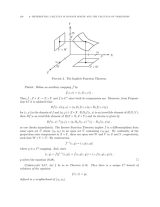
253. 9.4. HIGHER DERIVATIVES 253
Definition. Let X, Y be Banach spaces and f : X → Y . For n = 2, 3, . . . , define f to be
n-times Fréchet differentiable in a neighborhood of a point x if f is (n − 1)-times differentiable
in a neighborhood of x and the mapping x 7→ Dn−1f(x) is Fréchet differentiable near x. Define
Dn
f(x) = DDn−1
f(x) , n = 2, 3, . . . .
Notice that
f : X → Y ,
Df : X → B(X, Y ) ,
D2
f = D(Df) : X → B(X, B(X, Y )) = B2
(X, Y ) ,
.
.
.
Dn
f = D(Dn−1
f) : X → B(X, Bn−1
(X, Y )) = Bn
(X, Y ) .
We remark that, for n = 2 and f : X → Y , we must find D2f(x) ∈ B2(X, Y ) such that
kDf(x + h) − Df(x) − D2
f(x)(h)kB(X,Y ) = o(khkX) .
This is equivalent to showing
kDf(x + h)k − Df(x)k − D2
f(x)(h, k)kY = o(khkX)kkkX .
A similar remark holds for higher derivatives.
Examples. 1. If A ∈ B(X, Y ), then DA(x) = A for all x. Hence
D2
A(x) ≡ 0 for all x .
This is because
DA(x + h) − DA(x) ≡ 0
for all x.
2. Let X = H be a Hilbert space, F = R, and A ∈ B(H, H). Define f : H → R by
f(x) = (x, Ax)H .
Then, Df(x) = R((A+A∗)x), where R denotes the Riesz map. That is, Df(x) ∈ B(H, R) = H∗,
and for y ∈ H,
Df(x)(y) = (y, A∗
x + Ax)H .
To compute the second derivative, form the difference
[Df(x + h) − Df(x)]y = (y, (A + A∗
)(x + h) − (A + A∗
)x) = (y, (A + A∗
)h) ,
for y ∈ H. Thus it is determined that
D2
f(x)(y, h) = (y, (A + A∗
)h) .
Note that D2f(x) does not depend on x, so D3f(x) ≡ 0.
3. Let K ∈ L∞(I × I) where I = [a, b] ⊂ R. Define F : Lp(I) → Lp(I) by
F(g)(x) =
Z
I
K(x, y)gp
(y) dy
for p ∈ N and x ∈ I. Then, DF(g) ∈ B(Lp(I), Lp(I)) and
DF(g)h = p
Z
I
K(x, y)gp−1
(y)h(y) dy ,

254. 254 9. DIFFERENTIAL CALCULUS IN BANACH SPACES AND THE CALCULUS OF VARIATIONS
since the Binomial Theorem gives the expansion
F(g + h) − F(g) =
Z
I
K(x, y)[(g + h)p
− gp
] dy
=
Z
I
K(x, y)
pgp−1
(y)h(y) +
p
2
gp−2
(y)h2
(y) + · · ·
dy ,
wherein all but the first term is higher-order in h. Thus it follows readily that
DF(g + h)u − DF(g)u = p
Z
I
K(x, y)
(g + h)p−1
u − gp−1
u
dy
= p(p − 1)
Z
I
K(x, y)[gp−2
hu] dy + terms cubic in h, u .
It follows formally, and can be verified under strict hypotheses, that
D2
F(g)(h, k) = p(p − 1)
Z
I
K(x, y)gp−2
(y)h(y)k(y) dy .
Lemma 9.21 (Schwarz). Let X, Y be Banach spaces, U an open subset of X and f : U → Y
have two derivatives. Then D2f(x) is a symmetric bilinear mapping.
Proof. Consider the difference
g(h, k) = f(x + h + k) − f(x + h) − f(x + k) + f(x) − D2
f(x)(k, h) ,
so that
kD2
f(x)(h, k) − D2
f(x)(k, h)kY = kg(h, k) − g(k, h)kY
≤ kg(h, k) − g(0, k)kY + kg(0, k) − g(k, h)kY
= kg(h, k) − g(0, k)kY + kg(0, h) − g(k, h)kY
since g(0, k) = g(0, h) = 0. But the right-hand side of the last equality is bounded above by the
Mean Value Theorem as
kg(h, k) − g(0, k)kY ≤ sup kD1gkB(X,Y )khkX ,
kg(k, h) − g(0, h)kY ≤ sup kD1gkB(X,Y )kkkX .
Differentiate g partially with respect to the first variable h to obtain
D1g(h, k)h̃ = Df(x + h + k)h̃ − Df(x + h)h̃ − D2
f(x)(k, h̃)
= Df(x + h + k)h̃ − Df(x)h̃ − D2
f(x)(h + k, h̃)
− [Df(x + h)h̃ − Df(x)h̃ − D2
f(x)(h, h̃)] .
For khkX, kkkX small, it follows from the definition of the Fréchet derivative of Df that
kD1g(h, k)kB(X,Y ) = o(khkX + kkkX) .
Thus we have established that
kD2
f(x)(h, k) − D2
f(x)(k, h)kY = o(kkkX + khkX) (khkX + kkkX) ,
and it follows from bilinearity that in fact
D2
f(x)(h, k) = D2
f(x)(k, h)
for all h, k ∈ X [replace (h, k) by (h, k) and take → 0].

255. 9.4. HIGHER DERIVATIVES 255
Corollary 9.22. Let f, X, Y and U be as in Lemma 9.21, but suppose f has n ≥ 2
derivatives in U. Then Dnf(x) is symmetric under permutation of its arguments. That is, if π
is an n × n symmetric permutation matrix, then
Dn
f(x)(h1, . . . , hn) = Dn
f(x)(π(h1, . . . , hn)) .
Proof. This follows by induction from the fact that Dnf(x) = D2(Dn−2f)(x).
Theorem 9.23 (Taylor’s Formula). Let X, Y be Banach spaces, U ⊂ X open and suppose
f : U → Y has n derivatives throughout U. Then for x ∈ U and h small enough that x + h ∈ U,
f(x + h) = f(x) + Df(x)h +
1
2
D2
f(x)(h, h) + · · · +
1
n!
Dn
f(x)(h, . . . , h) + Rn(x, h) (9.29)
and
kRn(x, h)kY
khkn
X
−→ 0
as h → 0 in X, i.e., kRn(x, h)kY = o(khkn
X).
Proof. We first note in general that if F ∈ Bm(X, Y ) is symmetric and g is defined by
g(h) = F(h, . . . , h) ,
then
Dg(h)k = mF(h, . . . , h, k) .
This follows by straightforward calculation. For m = 1, F is just a linear map and the result is
already known. For m = 2, for example, just compute
g(h + k) − g(h) − 2F(h, k) = F(h + k, h + k) − F(h, h) − 2F(h, k) = F(k, k) ,
and
kF(k, k)kY ≤ Ckkk2
X ,
showing g is differentiable and that Dg(h) = 2F(h, ·).
For the theorem, the case n = 1 just reproduces the definition of f being differentiable at
x. We initiate an induction on n, supposing the result valid for all functions f satisfying the
hypotheses for k n, where n ≥ 2. Let f satisfy the hypotheses for k = n. Define Rn as in
(9.29) and notice that
D2Rn(x, h) = Df(x + h) − Df(x) − D2
f(x)(h, ·) − · · · −
1
(n − 1)!
Dn
f(x)(h, . . . , h, ·) .
That is,
Df(x + h) = Df(x) + D2
f(x)(h, ·) + · · · +
1
(n − 1)!
Dn
f(x)(h, . . . , h, ·) + D2Rn(x, h) ,
which is the (n − 1)st Taylor expansion of Df, and by induction we conclude that
kD2Rn(x, h)kB(X,Y )
khkn−1
X
−→ 0
as h → 0. On the other hand, by the Mean-Value Theorem, if khkX is sufficiently small, then
kRn(x, h)kY
khkn
X
=
kRn(x, h) − Rn(x, 0)kY
khkn
X
≤ sup
0≤α≤1
kD2Rn(x, αh)kB(X,Y )
khkn−1
X
−→ 0
as h → 0.

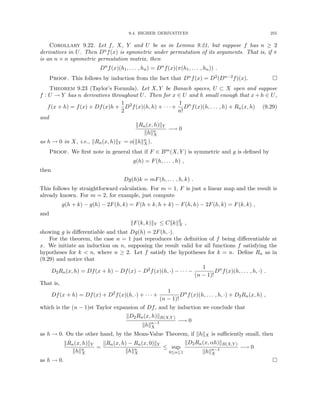
256. 256 9. DIFFERENTIAL CALCULUS IN BANACH SPACES AND THE CALCULUS OF VARIATIONS
9.5. Extrema
Definition. Let X be a set and f : X → R. A point x0 ∈ X is a minimum if f(x0) ≤ f(x)
for all x ∈ X; it is a maximum if f(x0) ≥ f(x) for all x ∈ X. An extrema is a point which is
a maximum or a minimum. If X has a topology, we say x0 is a relative (or local) minimum if
there is an open set U ⊂ X with x0 ∈ U such that
f(x0) ≤ f(x)
for all x ∈ U. Similarly, if
f(x0) ≥ f(x)
for all x ∈ U, then x0 is a relative maximum. If equality is disallowed above when x 6= x0, the
(relative) minimum or maximum is said to be strict.
Theorem 9.24. Let X be a NLS, let U be an open set in X and let f : U → R be differen-
tiable. If x0 ∈ U is a relative maximum or minimum, then Df(x0) = 0.
Proof. We show the theorem when x0 is a relative minimum; the other case is similar. We
argue by contradiction, so suppose that Df(x0) is not the zero map. Then there is some h 6= 0
such that Df(x0)h 6= 0. By possibly reversing the sign of h, we may assume that Df(x0)h 0.
Let t0 0 be small enough that x0 + th ∈ U for |t| ≤ t0 and consider for such t
1
t
[f(x0 + th) − f(x0)] =
1
t
[Df(x0)(th) + R1(x0, th)]
= Df(x0)h +
1
t
R1(x0, th) .
The quantity R1(x0, th)/t → 0 as t → 0. Hence for t1 ≤ t0 small enough and |t| ≤ t1,
1
t
R1(x0, th) ≤
1
2
|Df(x0)h| .
It follows that for |t| t1,
f(x0 + th) = f(x0) + t
Df(x0)h +
1
t
R1(x0, th)
f(x0) ,
provided we choose t 0. This contradiction proves the result for relative minima. Similar
ruminations establish the conclusion for relative maxima.
Definition. A critical point of a mapping f : U → Y , where U is open in X, is a point x0
where Df(x0) = 0. This is also referred to as a stationary point by some authors.
Corollary 9.25. If f : U → R is differentiable, then the relative extrema of f in U are
critical points of f.
Definition. Let X be a vector space over R, U ⊂ X a convex subset, and f : U → R. We
say that f is convex if whenever x1, x2 ∈ U and λ ∈ (0, 1), then
f(λx1 + (1 − λ)x2) ≤ λf(x1) + (1 − λ)f(x2) .
We say that f is concave if the opposite inequality holds. Moreover, we say that f is strictly
convex or concave if equality is not allowed above.
Proposition 9.26. Linear functionals on X are both convex and concave (but not strictly
so). If a, b 0 and f, g are convex, then af +bg is convex, and if at least one of f or g is strictly
convex, then so is af + bg. Furthermore, f is (strictly) convex if and only if −f is (strictly)
concave.

257. 9.5. EXTREMA 257
We leave the proof as an easy exercise of the definitions.
Proposition 9.27. Let X be a NLS, U a convex subset of X, and f : U → R convex and
differentiable. Then, for x, y ∈ U,
f(y) ≥ f(x) + Df(x)(y − x) ,
and, if Df(x) = 0, then x is a minimum of f in U. Moreover, if f is strictly convex, then for
x 6= y,
f(y) f(x) + Df(x)(y − x) ,
and Df(x) = 0 implies that f has a strict and therefore unique minimum.
Proof. By convexity, for λ ∈ [0, 1],
λf(y) + (1 − λ)f(x) ≥ f(x + λ(y − x)) ,
whence
f(y) − f(x) ≥
f(x + λ(y − x)) − f(x)
λ
.
Take the limit as λ → 0 on the right-hand side to obtain the desired result.
We leave the proof of the strictly convex case to the reader.
Example. Let Ω ⊂ Rd, f ∈ L2(Ω), and assume that the underlying field is real. Define
J : H1
0 (Ω) → R by
J(v) = 1
2k∇vk2
L2(Ω) − (f, v)L2(Ω) .
We claim that k∇vk2
L2(Ω) is strictly convex. To verify this, let v, w ∈ H1
0 (Ω) and λ ∈ (0, 1).
Then
k∇(λv + (1 − λ)w)k2
L2(Ω)
= λ2
k∇vk2
L2(Ω) + (1 − λ)2
k∇wk2
L2(Ω) + 2λ(1 − λ) (∇v, ∇w)L2(Ω)
= λk∇vk2
L2(Ω) + (1 − λ)k∇wk2
L2(Ω) − λ(1 − λ)[k∇vk2
L2(Ω) + k∇wk2
L2(Ω) − 2(∇v, ∇w)L2(Ω)]
= λk∇vk2
L2(Ω) + (1 − λ)k∇wk2
L2(Ω) − λ(1 − λ) (∇(v − w), ∇(v − w))L2(Ω)
λk∇vk2
L2(Ω) + (1 − λ)k∇wk2
L2(Ω) ,
unless v − w is identically constant on each connected component of Ω. As v − w ∈ H1
0 (Ω),
v = w on ∂Ω, and so v = w everywhere. That is, we have strict inequality whenever v 6= w, and
so we conclude that kvk2
L2(Ω) is strictly convex. By Prop. 9.26, we conclude that J(v) is also
strictly convex. Moreover,
DJ(u, v) = (∇u, ∇v)L2(Ω) − (f, v)L2(Ω) .
We conclude that u ∈ H1
0 (Ω) satisfies the boundary value problem
(∇u, ∇v)L2(Ω) = (f, v)L2(Ω)
if and only if u minimizes the “energy functional” J(v) over H1
0 (Ω):
J(u) J(v) for all v ∈ H1
0 (Ω), v 6= u .
Moreover, such a function u is unique.
Local convexity suffices to verify that a critical point is a relative extrema. More generally,
we can examine the second derivative.

258. 258 9. DIFFERENTIAL CALCULUS IN BANACH SPACES AND THE CALCULUS OF VARIATIONS
Theorem 9.28. If X is a NLS and f : X → R is twice differentiable at a relative minimum
x ∈ X, then
D2
f(x)(h, h) ≥ 0 for all h ∈ X .
Proof. By Taylor’s formula
f(x ± λh) = f(x) ± Df(x)λh + 1
2λ2
D2
f(x)(h, h) + o(λ2
khk2
X) ,
so we conclude that
D2
f(x)(h, h) = lim
λ→0
f(x + λh) + f(x − λh) − 2f(x)
λ2
≥ 0
if x is a local minimum.
Remark. In infinite dimensions, it is not the case that Df(x) = 0 and D2f(x)(h, h) 0
for all h 6= 0 implies that x is a local minimum. For example consider the function f : `2 → R
defined by
f(x) =
∞
X
k=1
1
k
− xk
x2
k ,
where x = (xk)∞
k=1 ∈ `2. Note that f is well defined on `2 (i.e., the sum converges). Direct
calculation shows that
Df(x)(h) =
∞
X
k=1
2
k
− 3xk
xkhk ,
D2
f(x)(h, h) =
∞
X
k=1
2
k
− 6xk
h2
k ,
so f(0) = 0, Df(0) = 0, and D2f(0)(h, h) 0 for all h 6= 0. However, let xk be the element of
`2 such that xk
j is 0 if j 6= k and 2/k if j = k. We compute that f(xk) 0, in spite of the fact
that xk → 0 as k → ∞. Thus 0 is not a local minimum of f.
Theorem 9.29 (Second Derivative Test). Let X be a NLS, and f : X → R have two
derivatives at a critical point x ∈ X. If there is some constant c 0 such that
D2
f(x)(h, h) ≥ ckhk2
X for all h ∈ X ,
then x is a strict local minimum point.
Proof. By Taylor’s Theorem, for any ε 0, there is δ 0 such that for khkX ≤ δ,
|f(x + h) − f(x) − 1
2D2
f(x)(h, h)| ≤ εkhk2
X ,
since the Taylor remainder is o(khk2
X). Thus,
f(x + h) − f(x) ≥ 1
2D2
f(x)(h, h) − εkhk2
X ≥ (1
2c − ε)khk2
X ,
and taking ε = c/4, we conclude that
f(x + h) ≥ f(x) + 1
4ckhk2
X ,
i.e., f has a local minimum at x.

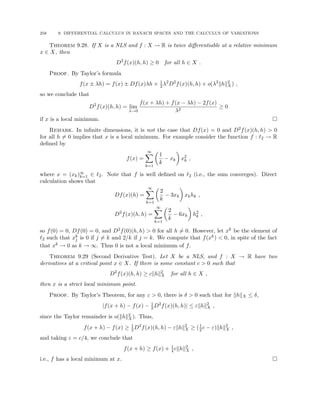
259. 9.6. THE EULER-LAGRANGE EQUATIONS 259
Remark. This theorem is not as general as it appears. If we define the bilinear form
(h, k)X = D2
f(x)(h, k) ,
we easily verify that, with the assumption of the Second Derivative Test, that in fact (h, k)X is
an inner product, which induces a norm equivalent to the original. Thus in fact X must be a
pre-Hilbert space, and it makes no sense to attempt use of the theorem when X is known not
to be pre-Hilbert.
9.6. The Euler-Lagrange Equations
A common problem in science and engineering applications is to find extrema of a functional
that involves an integral of a function. We will consider this situation via the following problem.
Let a b,
f : [a, b] × Rn
× Rn
→ R
and define the functional F : C1([a, b]) → R by
F(y) =
Z b
a
f(x, y(x), y0
(x)) dx .
With α and β given in Rn, let
C1
α,β([a, b], Rn
) = {v : [a, b] → Rn
| v has a continuous first derivative,
v(a) = α, and v(b) = β} .
Our goal is to find y ∈ C1
α,β([a, b], Rn) such that
F(y) = min
v∈C1
α,β([a,b],Rn)
F(v) .
Example. Find y(x) ∈ C1([a, b]) such that y(a) = α 0 and y(b) = β 0 and the surface
of revolution of the graph of y about the x-axis has minimal area. Recall that a differential of
arc length is given by
ds =
p
1 + (y0(x))2 dx ,
so our area as a function of the curve y is
A(y) =
Z b
a
2πy(x)
p
1 + (y0(x))2 dx , (9.30)
since clearly y(x) ≥ 0 for all x ∈ [a, b].
If α and β are zero, C1
0,0([a, b], Rn) = C1
0 ([a, b], Rn) is a Banach space with the W1,1([a, b])
(Sobolev space) maximum norm, and our minimum is found at a critical point. However, in
general C1
α,β([a, b], Rn) is not a linear vector space. Rather it is an affine space, a translate of a
vector space. To see this, let
`(x) =
1
b − a
[α(b − x) + β(x − a)]
be the linear function connecting (a, α) to (b, β). Then
C1
α,β([a, b], Rn
) = C1
0 ([a, b], Rn
) + ` .
To solve our problem, then, we need to consider any fixed element of C1
α,β, such as `(x), and
all possible “admissible variations” h of it that lie in C1
0 ; that is, we minimize F(v) by searching

260. 260 9. DIFFERENTIAL CALCULUS IN BANACH SPACES AND THE CALCULUS OF VARIATIONS
among all possible “competing functions” v = ` + h ∈ C1
α,β, where h ∈ C1
0 , for the one that
minimizes F(v), if any. On C1
0 , we can find the derivative of F(` + h) as a function of h, and
thereby restrict our search to the critical points. We call such a point y = ` + h a critical point
for F defined on C1
α,β. We present a general result on the derivative of F of the form considered
in this section.
Theorem 9.30. If f ∈ C1([a, b] × Rn × Rn) and
F(y) =
Z b
a
f(x, y(x), y0
(x)) dx ,
then F : C1([a, b]) → R is continuously differentiable and
DF(y)(h) =
Z b
a
[D2f(x, y(x), y0
(x)) h(x) + D3f(x, y(x), y0
(x)) h0
(x)] dx
for all h ∈ C1([a, b]).
Proof. Let A be defined by
Ah =
Z b
a
[D2f(x, y(x), y0
(x)) h(x) + D3f(x, y(x), y0
(x)) h0
(x)] dx ,
which is clearly a bounded linear functional on C1, since the norm of any v ∈ C1 is
kvk = max(kvkL∞ , kv0
kL∞ ) .
Now
F(y + h) − F(y) =
Z b
a
Z 1
0
d
dt
f(x, y + th, y0
+ th0
) dt dx
=
Z b
a
Z 1
0
D2f(x, y + th, y0
+ th0
) h + D3f(x, y + th, y0
+ th0
) h0
dt dx ,
so
|F(y + h) − F(y) − Ah| ≤
Z b
a
Z 1
0
|[D2f(x, y + th, y0
+ th0
) − D2f(x, y, y0
)] h| dt dx
+
Z b
a
Z 1
0
|[D3f(x, y + th, y0
+ th0
) − D3f(x, y, y0
)] h0
| dt dx .
Since D2f and D3f are uniformly continuous on compact sets, the right-hand side is o(khk),
and we conclude that DF(y) = A.
It remains to show that DF(y) is continuous. But this follows from uniform continuity of
D2f and D3f, and from the computation
|DF(y + h)k − DF(y)k| ≤
Z b
a
|[D2f(x, y + h, y0
+ h0
) − D2f(x, y, y0
)] k| dx
+
Z b
a
|[D3f(x, y + h, y0
+ h0
) + D3f(x, y, y0
)] k0
| dx ,
which tends to 0 as khk → 0 for any k ∈ C1([a, b]) with kkk ≤ 1.

261. 9.6. THE EULER-LAGRANGE EQUATIONS 261
Theorem 9.31. Suppose f ∈ C1([a, b] × Rn × Rn), y ∈ C1
α,β([a, b]), and
F(y) =
Z b
a
f(x, y(x), y0
(x)) dx .
Then y is a critical point for F if and only if the curve x 7→ D3f(x, y(x), y0(x)) is C1([a, b]) and
y satisfies the Euler-Lagrange Equations
D2f(x, y, y0
) −
d
dx
D3f(x, y, y0
) = 0 .
In component form, the Euler-Lagrange Equations are
∂f
∂yk
=
d
dx
∂f
∂y0
k
, k = 1, ..., n ,
or
fyk
=
d
dx
fy0
k
, k = 1, ..., n .
The converse implication of the Theorem is easily shown from the previous result after
integrating by parts, since h ∈ C1
0 . The direct implication follows easily from the previous result
and the following Lemma, which can be proved by classical methods, but is also trivial to prove
from the Lebesgue Lemma 5.7. We leave the details to the reader.
Lemma 9.32 (Dubois-Reymond). Let ϕ and ψ lie in C0([a, b], Rn). Then
(i)
R b
a ϕ(x) · h0(x) dx = 0 for all h ∈ C1
0 if and only if ϕ is identically constant.
(ii)
R b
a [ϕ(x) · h(x) + ψ(x) · h0(x)] dx = 0 for all h ∈ C1
0 if and only if ψ ∈ C1 and ψ0 = ϕ.
Proof. Both converse implications are trivial after integrating by parts. For the direct
implication of (i), let
ϕ̄ =
1
b − a
Z b
a
ϕ(x) dx ,
and note that then
0 =
Z b
a
ϕ(x) · h0
(x) dx =
Z b
a
(ϕ(x) − ϕ̄) · h0
(x) dx .
Take
h =
Z x
a
(ϕ(s) − ϕ̄) ds ∈ C1
0 ,
so that h0 = ϕ − ϕ̄. We thereby demonstrate that
kϕ − ϕ̄kL2 = 0 ,
and conclude that ϕ = ϕ̄ (almost everywhere, but both functions are continuous, so everywhere).
For the direct implication of (ii), let
Φ =
Z x
a
ϕ(s) ds ,
so that Φ0 = ϕ. Then the hypothesis of (ii) shows that
Z b
a
[Φ − ψ] · h0
dx =
Z b
a
[Φ · h0
(x) + ϕ · h] dx =
Z b
a
d
dx
(Φ · h) dx = 0 ,

262. 262 9. DIFFERENTIAL CALCULUS IN BANACH SPACES AND THE CALCULUS OF VARIATIONS
since h vanishes at a and b. We conclude from (i) that Φ − ψ is constant. Since Φ is C1, so is
ψ, and ψ0 = Φ0 = ϕ.
Definition. Solutions of the Euler-Lagrange equations are called extremals.
Example. We illustrate the theory by finding the shortest path between two points. Suppose
y(x) is a path in C1
α,β([a, b]), which connects (a, α) to (b, β). Then we seek to minimize the length
functional
L(y) =
Z b
a
p
1 + (y0(x))2 dx
over all such y. The integrand is
f(t, y, y0
) =
p
1 + (y0(x))2 ,
so the Euler-Lagrange equations become simply
(D3f)0
= 0 ,
and so we conclude that for some constant c,
y0(x)
p
1 + (y0(x))2
= c .
Thus,
y0
(x) = ±
r
c2
1 − c2
,
if c2 6= 1, and there is no solution otherwise. In any case, y0(x) is constant, so the only critical
paths are lines, and there is a unique such line in C1
α,β([a, b]). Since L(y) is convex, this path is
necessarily a minimum, and we conclude the well-known maxim: the shortest distance between
two points is a straight line.
Example. Many problems have no solutions. For example, consider the problem of min-
imizing the length of the curve y ∈ C1([0, 1]) such that y(0) = y(1) = 0 and y0(0) = 1. The
previous example shows that extremals would have to be lines. But there is no line satisfying
the three boundary conditions, so there are no extremals. Clearly the minimum approaches 1,
but is never attained by a C1-function.
It is generally not easy to solve the Euler-Lagrange equations. They constitute a nonlinear
second order ordinary differential equation for y(x). To see this, suppose that y ∈ C2([a, b]) and
compute
D2f = (D3f)0
= D1D3f + D2D3f y0
+ D2
3f y00
.
We note that D2
3f(x, y, y0) ∈ B2(Rn, R), which is isomorphic to B(Rn, Rn), so, provided D2
3f(x, y, y0)
is invertible,
y00
= (D2
3f)−1
(D2f − D1D3f − D2D3f y0
) .
Definition. If y is an extremal and D2
3f(x, y, y0) is invertible for all x ∈ [a, b], then we call
y a regular extremal.
Proposition 9.33. If f ∈ C2([a, b]×Rn ×Rn) and y ∈ C1([a, b]) is a regular extremal, then
y ∈ C2([a, b]).
In this case, we can reduce the problem to first order.

263. 9.6. THE EULER-LAGRANGE EQUATIONS 263
Theorem 9.34. If f ∈ C2([a, b] × Rn × Rn), f(x, y, z) = f(y, z) only, and y ∈ C1([a, b]) is
a regular extremal, then D3f y0 − f is constant.
Proof. Simply compute
(D3f y0
− f)0
= D3f y00
+ (D3f)0
y0
− f0
= D3f y00
+ D2f y0
− (D2f y0
+ D3f y00
) = 0 ,
using the Euler-Lagrange equation for the extremal.
Example. We reconsider the problem of finding y(x) ∈ C1([a, b]) such that y(a) = α 0
and y(b) = β 0 and the surface of revolution of the graph of y about the x-axis has minimal
area. The area as a function of the curve is given in (9.30), so
f(y, y0
) = 2πy(x)
p
1 + (y0(x))2 .
Note that
D2
3f(y, y0
) =
2πy(x)
(1 + (y0(x))2)3/2
6= 0 ,
unless y(x) = 0. Clearly y(x) 0, so our extremals are regular, and we can use the theorem to
find them. For some constant C,
2πy (y0)2
(1 + (y0)2)1/2
− 2πy(1 + (y0
)2
)1/2
= 2πC ,
which implies that
y0
=
1
C
p
y2 − C2 .
Applying separation of variables, we need to integrate
dy
p
y2 − C2
=
dx
C
,
which, for some constant λ, gives us the solution
y(x) = C cosh(x/C + λ) ,
which is called a catenary. Suppose that a = 0, so that C = α/ cosh λ and
y(b) = β =
α
cosh λ
cosh
cosh λ
α
b + λ
.
That is, we determine C once we have λ, which must solve the above equation. There may or
may not be solutions λ (i.e., there may not be regular extremals). It is a fact, which we will
not prove (see [Sa, pp. 62ff.]), that the minimal area is given either by a regular extremal or
the Goldschmidt solution, which is the piecewise graph that uses straight lines to connect the
points (0, α) to (0, 0), (0, 0) to (b, 0), and finally (b, 0) to (b, β). This is not a C1 curve, so it is
technically inadmissible, but it has area AG = π(α2 +β2). If there are no extremals, then, given
0, we have C1 curves approximating the Goldschmidt solution such that the area is greater
than but within of AG.
Example (The Brachistochrone problem with a free end). Sometimes one does not impose
a condition at one end. An example is the Brachistochrone problem. Consider a particle moving
under the influence of gravity in the xy-plane, where y points upwards. We assume that the
particle starts from rest at the position (0, 0) and slides frictionlessly along a curve y(x), moving

264. 264 9. DIFFERENTIAL CALCULUS IN BANACH SPACES AND THE CALCULUS OF VARIATIONS
t
b
t
β
S
S
S
S
S
S
S
S
S
θ
dx
dy
ds
Figure 3. The Brachistochrone problem.
in the x-direction a distance b 0 and falling an unspecified distance (see Fig. 3). We wish to
minimize the total travel time. Let the final position be (b, β), where β 0 is unspecified. We
assume that the curve y ∈ C1
∗ ([0, b]), where
C1
∗ ([a, b]) = {v ∈ C1
([a, b]) : v(a) = 0} .
The steeper the curve, the faster it will move; however, it must convert some of this speed into
motion in the x-direction to travel distance b. To derive the travel time functional T(y), we
note that Newton’s Law implies that for a mass m traveling on the arc s with angle θ from the
downward direction (see Fig. 3),
m
d2s
dt2
= −mg cos θ = −mg
dy
ds
,
where g is the gravitational constant. The mass cancels and
1
2
d
dt
ds
dt
2
=
d2s
dt2
ds
dt
= −g
dy
dt
,
so we conclude that for some constant C,
ds
dt
2
= −2gy + C .
But at t = 0, both the speed and y(0) are zero, so C = 0, and
ds
dt
=
p
−2gy .
Now the travel time is given by
T(y) =
Z
dt =
Z
ds
√
−2gy
=
Z b
0
s
1 + (y0(x))2
−2gy(x)
dx .
We need a general result to deal with the free end.
Theorem 9.35. If y ∈ C2([a, b]) minimizes
F(y) =
Z b
a
f(x, y(x), y0
(x)) dx
subject only to the single constraint that y(a) = α ∈ R, then y must satisfy the Euler Lagrange
equations and D3f(b, y(b), y0(b)) = 0.

265. 9.7. CONSTRAINED EXTREMA AND LAGRANGE MULTIPLIERS 265
Proof. We simply compute for y ∈ C1
∗ ([a, b]) + α and h ∈ C1
∗ ([a, b])
DF(y) h =
Z b
a
(D2f h + D3f h0
) dx =
Z b
a
(D2f h − (D3f)0
h) dx + D3f(b, y(b), y0
(b)) h(b) .
If h ∈ C1
0,0([a, b]), we derive the Euler-Lagrange equations, and otherwise we obtain the second
condition at x = b.
Example (The Brachistochrone problem with a free end, continued). Since we are looking
for a minimum, we can drop the factor
√
2g and concentrate on
f(y, y0
) =
s
1 + (y0(x))2
−y(x)
.
This is independent of x, so we solve
y0
D3f − f = C1 =
1
√
−y
(y0)2
p
1 + (y0)2
−
p
1 + (y0)2
,
or
Z s
−y
C−2
1 + y
dy = x − C2 .
This is solved using a trigonometric substitution, so we let
y = −C−2
1 sin2
(φ/2) = −(1 − cos φ)/2C2
1 ,
where 0 ≤ φ ≤ π, and then
x = −(φ − sin φ)/2C2
1 + C2 .
Applying the initial condition (φ = 0), we determine that the curve is
(x, y) = C(φ − sin φ, 1 − cos φ)
for some constant C. This is a cycloid. Now C is determined by the auxiliary condition
0 = D3f(y(b), y0
(b)) =
1
p
y(b)
y0(b)
p
1 + (y0(b))2
,
which requires
0 = y0
(b) =
dy
dφ
dx
dφ
−1
=
sin φ(b)
1 − cos φ(b)
.
Thus φ(b) = π (since φ ∈ [0, π]), so C = b/π and the solution is complete.
9.7. Constrained Extrema and Lagrange Multipliers
When discussing the Euler-Lagrange equations, we considered the problem of finding relative
extrema of a nonlinear functional in C1
α,β, which is an affine translate of a Banach space. We can
phrase this differently: we found extrema in the Banach space C1 subject to the linear constraint
that the function agrees with α and β at its endpoints. We consider now the more general
problem of finding relative extrema of a nonlinear functional subject to a possibly nonlinear
constraint.
Let X be a Banach space, U ⊂ X open, and f : U → R. To describe our constraint, we
assume that there are functions gi : X → R for i = 1, ..., m that define the set M ⊂ U by
M = {x ∈ U : gi(x) = 0 for all i} .

266. 266 9. DIFFERENTIAL CALCULUS IN BANACH SPACES AND THE CALCULUS OF VARIATIONS
Our problem is to find the relative extrema of f restricted to M. Note that M is not necessarily
open, so we must discuss what happens on ∂M. To rephrase our problem: Find the relative
extrema of f(x) on U subject to the constraints
g1(x) = ... = gm(x) = 0 . (9.31)
To find the relative extrema of f(x) on U subject to the constraints (9.31), we can instead
solve an unconstrained problem, albeit in more dimensions. Define H : X × Rm → R by
H(x, λ) = f(x) + λ1g1(x) + ... + λmgm(x) . (9.32)
The critical points of H are given by solving for a root of the system of equations defined by
the partial derivatives
D1H(x, λ) = Df(x) + λ1Dg1(x) + ... + λmDgm(x) ,
D2H(x, λ) = g1(x) ,
.
.
.
Dm+1H(x, λ) = gm(x) .
Such a critical point satisfies the m constraints and an additional condition which is necessary
for an extrema, as we prove below.
Theorem 9.36 (Lagrange Multiplier Theorem). Let X be a Banach space, U ⊂ X open,
and f, gi : U → R, i = 1, ..., m, be continuously differentiable. If x ∈ M is a relative extrema for
f|M , where
M = {x ∈ U : gi(x) = 0 for all i} ,
then there is a nonzero λ = (λ0, ..., λm) ∈ Rm+1 such that
λ0Df(x) + λ1Dg1(x) + ... + λmDgm(x) = 0 . (9.33)
That is, to find a local extrema in M, we need only consider points that satisfy (9.33). We
search through the unconstrained space U for such points x, and then we must verify that in
fact x ∈ M holds. Two possibilities arise for x ∈ U. If {Dgi(x)}m
i=1 is linearly independent,
the only nontrivial way to satisfy (9.33) is to take λ0 6= 0. Otherwise, {Dgi(x)}m
i=1 is linearly
dependent, and (9.33) is satisfied for a nonzero λ with λ0 = 0.
Our method of search then is clear. (1) First we find critical points of H as defined above in
(9.32). These points automatically satisfy both (9.33) and x ∈ M. These points are potential
relative extrema. (2) Second, we find points x ∈ U where {Dgi(x)}m
i=1 is linearly dependent.
Then (9.33) is satisfied, so we must further check to see if indeed x ∈ M, i.e., each gi(x) = 0.
If so, x is also a potential relative extrema. (3) Finally, we determine if the potential relative
extrema are indeed extrema or not. Often, the constraints are chosen so that {Dgi(x)}m
i=1 is
always linearly independent, and the second step does not arise. (We remark that if we want
extrema on M̄, then we would also need to check points on ∂M.)
Proof of the Lagrange Multiplier Theorem. Suppose that x is a local minimum of
f|M ; the case of a local maximum is similar. Then we can find an open set V ⊂ U such that
x ∈ V and
f(x) ≤ f(y) for all y ∈ M ∩ V .
Define F : V → Rm+1 by
F(y) = (f(y), g1(y), ..., gm(y)) .

267. 9.7. CONSTRAINED EXTREMA AND LAGRANGE MULTIPLIERS 267
Since x is a local minimum on M, for any ε 0,
(f(x) − ε, 0, ..., 0) 6= F(y) for all y ∈ V .
Thus, we conclude that F does not map V onto an open neighborhood of F(x) = (f(x), 0, ..., 0) ∈
Rm+1.
Suppose that DF(x) maps X onto Rm+1. Then construct a space X̃ = span{v1, ..., vm+1} ⊂
X where we choose each vi such that DF(x)(vi) = ei, the standard unit vector in the ith
direction in Rm+1. Let X̂ = {v ∈ X̃ : x + v ∈ V }, and define the function h : X̂ → Rm+1 by
h(v) = F(x+v). Now Dh(0) = DF(x) maps X̃ onto Rm+1 is invertible, so the Inverse Function
Theorem implies that h maps an open subset S of X̂ containing 0 onto an open subset of Rm+1
containing h(0) = F(x). But then x + S ⊂ V is an open set that contradicts our previous
conclusion regarding F.
Thus DF(x) cannot map onto all of Rm+1, and so it maps onto a proper subspace. There
then is some nonzero vector λ ∈ Rm+1 orthogonal to DF(x)(X). Thus
λ0Df(x)(y) + λ1Dg1(x)(y) + ... + λmDgm(x)(y) = 0 ,
for any y ∈ X, and we conclude that this linear conbination of the operators must vanish, i.e.,
(9.33) holds.
Note that this theorem is especially useful when the function F and constraints Gi are given
as integral operators, i.e., when
F(y) =
Z b
a
f(x, y, y0
) dx and Gi(y) =
Z b
a
gi(x, y, y0
) dx .
In that case,
H(y, λ) =
Z b
a
hλ(x, y, y0
) dx ,
where
hλ(x, y, y0
) = f(x, y, y0
) +
m
X
i=1
λigi(x, y, y0
) ,
and the Euler-Lagrange equations can be used to find the extrema:
Dyhλ(x, y, y0
) =
d
dx
Dy0 hλ(x, y, y0
) .
In the previous section we had boundary conditions. It may be best to impose such point
constraints directly, as in the following example.
Example. The Isoperimetric Problem can be stated as follows: among all rectifiable curves
in R2
+ from (−1, 0) to (1, 0) with length `, find the one enclosing the greatest area. We need to
maximize the functional
A(u) =
Z 1
−1
u(t) dt
subject to the constraint
L(u0
) =
Z 1
−1
p
1 + (u0(t))2 dt = `

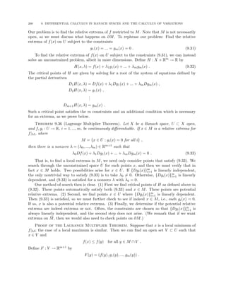
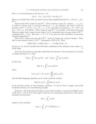
268. 268 9. DIFFERENTIAL CALCULUS IN BANACH SPACES AND THE CALCULUS OF VARIATIONS
over the set u ∈ C1
0,0([−1, 1]) with u ≥ 0. Let
H(u, λ) = A(u) + λ[L(u0
) − `] =
Z 1
−1
hλ(u, u0
) dt ,
where
hλ(u, u0
) = u + λ
p
1 + (u0(t))2 − `/2
.
To find a critical point of the system, we need to find both DuH and DλH. For the former, it is
given by considering λ fixed and solving the Euler-Lagrange equations: D2hλ = (D3hλ)0. That
is,
1 = λ
d
dt
u0
p
1 + (u0(t))2
!
,
so for some constant C1,
t = λ
u0
p
1 + (u0(t))2
+ C1 .
Solving for u0 yields
u0
(t) =
t − C1
p
λ2 − (t − C1)2
.
Another integration gives a constant C2 and
u(t) =
p
λ2 − (t − C1)2 + C2 ,
or, rearranging, we obtain the equation of a circular arc
(u(t) − C2)2
+ (t − C1)2
= λ2
with center (C1, C2) of radius λ. The partial derivative DλH simply recovers the constraint that
the arc length is `, and the requirement that u ∈ C0,0([−1, 1]) says that it must go through the
points u(−1) = (−1, 0) and u(1) = (1, 0). We leave it to the reader to complete the example
by showing that these conditions uniquely determine C1 = 0, C2, and λ =
p
1 + C2
2 , where C2
satisfies the transcendental equation
q
1 + C2
2 =
`
2[π − tan−1(1/C2)]
.
Moreover, the reader may justify that a maximum is obtained at this critical point.
We also need to check the condition DL(u0) = 0. Again the Euler-Lagrange equations allow
us to find these points easily. The result, left to the reader, is that for some constant C of
integration,
u0
=
C
√
1 − C
,
which means that u is a straight line. The fixed ends imply that u ≡ 0, and so we do not satisfy
the length constraint unless ` = 2, a trivial case to analyze.
As a corollary, among curves of fixed lengths, the circle encloses the region of greatest area.

269. 9.8. LOWER SEMI-CONTINUITY AND EXISTENCE OF MINIMA 269
9.8. Lower Semi-Continuity and Existence of Minima
Whether there exists a minimum of a functional is an important question. If a minimum
exists, we can locate it by analyzing critical points. Perhaps the simplest criterion for the
existence of a minimum is to consider convex functionals, as we have done previously. Next
simplest is perhaps to note that a continuous function on a compact set attains its minimum.
However, in an infinite dimensional Banach space X, bounded sets are not compact; that
is, compact sets are very small. This observation suggests that, at least when X is reflexive,
we consider using the weak topology, since then the Banach-Alaoglu Theorem 2.51 implies that
bounded sets are weakly compact. The problem now is that many interesting functionals are
not weakly continuous, such as the norm itself. For the norm, it is easily seen that:
If un
w
* u, then lim inf
n→∞
kunk ≥ kuk ,
with inequality possible. We are lead to consider a weaker notion of continuity.
Definition. Let X be a topological space. A function f : X → (−∞, ∞] is said to be lower
semicontinuous (l.s.c.) if whenever limn→∞ xn = x, then
lim inf
n→∞
f(xn) ≥ f(x) .
Proposition 9.37. Let X be a topological space and f : X → (−∞, ∞]. Then f is lower
semicontinuous if and only if the sets
Aα = {x ∈ X : f(x) ≤ α}
are closed for all α ∈ R.
Proof. Suppose f is l.s.c. Let xn ∈ Aα be such that xn → x ∈ X. Then
f(x) ≤ lim inf
n→∞
f(xn) ≤ α ,
so x ∈ Aα and Aα is closed.
Suppose now each Aα is closed. Then
Ac
α = {x ∈ X : f(x) α}
is open. Let xn → x ∈ X, and suppose that x ∈ Ac
α for some α (i.e., f(x) α). Then there is
some Nα 0 such that for all n ≥ Nα, xn ∈ Ac
α, and so lim infn→∞ f(xn) ≥ α. In other words,
whenever f(x) α, lim infn→∞ f(xn) ≥ α, so we conclude that
lim inf
n→∞
f(xn) ≥ sup{α : f(x) α} = f(x) .
Theorem 9.38. If M is compact and f : M → (−∞, ∞] is lower semicontinuous, then f is
bounded below and takes on its minumum value.
Proof. Let
A = inf
x∈M
f(x) ∈ [−∞, ∞] .
If A = −∞, choose a sequence xn ∈ M such that f(xn) ≤ −n for all n ≥ 1. Since M is compact,
there is x ∈ M such that, for some subsequence, xni → x as i → ∞. But
f(x) ≤ lim inf
i→∞
f(xni ) = −∞ ,
contradicting that f maps into (−∞, ∞]. Thus A −∞, and f is bounded below.

270. 270 9. DIFFERENTIAL CALCULUS IN BANACH SPACES AND THE CALCULUS OF VARIATIONS
Now choose a sequence xn ∈ M such that f(xn) ≤ A + 1/n, and again extract a convergent
subsequence xni → x ∈ M as i → ∞. We compute
A ≤ f(x) ≤ lim inf
i→∞
f(xni ) ≤ lim inf
i→∞
(A + 1/n) = A ,
and we conclude that f(x) = A attains its minimum at x.
The previous results apply to general topological spaces. For reflexive Banach spaces, we
have both the strong (or norm) and weak topologies.
Theorem 9.39. Let M be a weakly closed subspace of a reflexive Banach space X. If f :
M → (−∞, ∞] is weakly lower semicontinuous and, for some α, Aα = {x ∈ X : f(x) ≤ α} is
bounded and nonempty, then f is bounded from below and there is some x0 ∈ M such that
f(x0) = min
x∈M
f(x) .
Proof. By the Banach-Alaoglu Theorem 2.51, Āα is compact, so f|Āα
attains its minimum.
But for x ∈ M Āα, f(x) α ≥ minx∈Āα
f(x), and the theorem follows.
It is important to determine when a function is weakly lower semicontinuous. The following
requirement is left to the reader, and its near converse follows.
Proposition 9.40. If X is a Banach space and f : X → (−∞, ∞] is weakly lower semicon-
tinuous, then f is strongly lower semicontinuous.
Theorem 9.41. Suppose X is a Banach space and f : X → (−∞, ∞]. If V = {x ∈ X :
f(x) ∞} is a subspace of X, and if f is both convex on V and strongly lower semicontinuous,
then f is weakly lower semicontinuous.
Proof. For α ∈ R, let Aα = {x ∈ X : f(x) ≤ α} be as usual. Since f is strongly l.s.c.,
Prop. 9.37 implies that Aα is closed in the strong (i.e., norm) topology. But f being convex on V
implies that Aα is also convex. A strongly closed convex set is weakly closed (see Corollary 2.57),
so we conclude that f is weakly l.s.c.
Lemma 9.42. Let f : C → [0, ∞) be convex, Ω a domain in Rd, and 1 ≤ p ∞. Then
F : Lp(Ω) → [0, ∞], defined by
F(u) =
Z
Ω
f(u(x)) dx ,
is norm and weak l.s.c.
Proof. Since F is convex, it is enough to prove the norm l.s.c. property. Let un → u in
Lp(Ω) and choose a subsequence such that
lim
i→∞
F(uni ) = lim inf
n→∞
F(un)
and uni (x) → u(x) for almost every x ∈ Ω. Then f(uni (x)) → f(u(x)) for a.e. x, since f being
convex is also continuous. Fatou’s lemma finally implies that
F(u) ≤ lim inf
i→∞
F(uni ) = lim inf
n→∞
F(un) .
Corollary 9.43. If Ω is a domain in Rd and 1 ≤ p, q ∞, then the Lq(Ω)-norm is weakly
l.s.c. on Lp(Ω).

271. 9.8. LOWER SEMI-CONTINUITY AND EXISTENCE OF MINIMA 271
We close this section with two examples that illustrate the concepts.
Example. Let f ∈ C∞
0 (Rn) and consider the differential equation
−∆u + u|u| + u = f .
Let us show that there is a solution. Let
F(u) =
Z
Rd
1
2|∇u|2
+ 1
3|u|3
+ 1
2|u|2
− fu
dx ,
which may be +∞ for some u. Now if v ∈ C∞
0 (Rd),
DF(u)(v) =
Z
Rd
∇u · ∇v + |u|uv + uv − fv
dx
=
Z
Rd
− ∆u + u|u| + u − f
v dx
which vanishes if and only if the differential equation is satisfied. Since F is clearly convex, there
will be a solution to the differential equation if F takes on its minimum.
Now
F(u) ≥ 1
2k∇uk2
L2(Rd) − kfkL2(Rd)kukL2(Rd) ≥ 1
4k∇uk2
L2(Rd) − kfk2
L2(Rd) ,
so the set {u ∈ L2(Rd) : F(u) ≤ 1} is bounded by 4(1 + kfk2
L2(Rd)
), and nonempty (since it
contains u ≡ 0). We will complete the proof if we can show that F is l.s.c.
The last term of F is weakly continuous, and the second and third terms are weakly l.s.c.,
since they are norm l.s.c. and the space is convex. For the first term, let un
w
* u in L2. Then
k∇ukL2 = sup
ψ∈(C∞
0 )d, kψkL2 =1
|(ψ, ∇u)L2 |
= sup
ψ∈(C∞
0 )d, kψkL2 =1
|(∇ · ψ, u)L2 |
≤ sup
ψ∈(C∞
0 )d, kψkL2 =1
lim
n→∞
|(∇ · ψ, un)L2 |
= sup
ψ∈(C∞
0 )d, kψkL2 =1
lim
n→∞
|(ψ, ∇un)L2 |
≤ lim inf
n→∞
k∇unkL2
by Cauchy-Schwartz. Thus the first term is l.s.c. as well.
Example (Geodesics). Let M ⊂ Rd be closed and let γ : [0, 1] → M be a rectifiable curve
(i.e., γ is continuous and γ0, as a distribution, is in L1([0, 1]; Rd)). The length of γ is
L(γ) =
Z 1
0
|γ0
(s)| ds .
Theorem 9.44. Suppose M ⊂ Rd be closed. If x, y ∈ M and there is at least one rectifiable
curve γ : [0, 1] → M with γ(0) = x and γ(1) = y, then there exists a rectifiable curve γ̃ : [0, 1] →
M such that γ̃(0) = x, γ̃(1) = y, and
L(γ̃) = inf{L(γ)|γ : [0, 1] → M is rectifiable and γ(0) = x, γ(1) = y} .
Such a minimizing curve is called a geodesic.

272. 272 9. DIFFERENTIAL CALCULUS IN BANACH SPACES AND THE CALCULUS OF VARIATIONS
Note that a geodesic is the shortest path on some manifold M (i.e., surface in Rd) between
two points. One exists provided only that the two points can be joined within M. Note that
a geodesic may not be unique (e.g., consider joining points (−1, 0) and (1, 0) within the unit
circle).
Proof. We would like to use Theorem 9.39; however, L1 is not reflexive. We need two key
ideas to resolve this difficulty. We expect that γ0 is constant along a geodesic, so define
E(γ) =
Z 1
0
|γ0
(s)|2
ds
and let us try to minimize E in L2([0, 1]). This is the first key idea.
Define
Y =
f ∈ L2
([0, 1]; Rd
) : γf (s) ≡ x +
Z s
0
f(t) dt ∈ M for all s ∈ [0, 1] and γf (1) = y
.
These are the derivatives of rectifiable curves from x to y. Since the map f 7→
R s
0 f(t) dt
is a continuous linear functional, Y is weakly closed in L2([0, 1]; Rd). Since γ0
f = f, define
Ẽ : Y → [0, ∞) by
Ẽ(f) = E(γf ) =
Z 1
0
|f(s)|2
ds .
Clearly | · | is convex, so Ẽ is weakly l.s.c. by Lemma 9.42. Let
Aα = {f ∈ Y : Ẽ(f) ≤ α} ,
so that by definition Aα is bounded for any α. If Aα is not empty for some α, then there is a
minimizer f0 of Ẽ, by Theorem 9.39.
Now we need the second key idea. Given any rectifiable γ, define its geodesic reparameteri-
zation γ∗ by
T(s) =
1
L(γ)
Z s
0
|γ0
(t)| dt ∈ [0, 1] and γ∗
(T(s)) = γ(s) ,
which is well defined since T is nondecreasing and T(s) is constant only where γ is also constant.
But
γ0
(s) = γ∗
(T(s))
0
= γ∗0
(T(s)) T0
(s) = γ∗0
(T(s))
|γ0(s)|
L(γ)
,
so
|γ∗0
(s)| = L(γ)
is constant. Moreover, L(γ∗) = L(γ), and so
E(γ∗
) = L(γ∗
)2
.
Now at least one γ exists by hypothesis, so the reparameterized γ∗ has E(γ∗) ∞. Thus,
for some α, Aα is nonempty, and we conclude that we have a minimizer f0 of Ẽ.
Finally, for any rectifiable curve,
E(γ) ≥ L(γ)2
= L(γ∗
)2
= E(γ∗
) .
Thus a curve of minimal energy E must have |γ0| constant. So, for any rectifiable γ = γf (where
f = γ0),
L(γ) = E(γ∗)1/2
= Ẽ(f)1/2
≥ Ẽ(f0)1/2
= E(γf0 )1/2
= L(γf0 ) ,

273. 9.9. EXERCISES 273
and γf0 is our geodesic.
9.9. Exercises
1. Let X, Y1, Y2, and Z be normed linear spaces and P : Y1 × Y2 → Z be a continuous bilinear
map (so P is a “product” between Y1 and Y2).
(a) Show that for yi, ŷi ∈ Yi,
DP(y1, y2)(ŷ1, ŷ2) = P(y1, ŷ2) + P(ŷ1, y2) .
(b) If f : X → Y1 × Y2 is differentiable, show that for h ∈ X,
D(P ◦ f)(x) h = P(Df1(x) h, f2(x)) + P(f1(x), Df2(x) h) .
2. Let X be a real Hilbert space and A1, A2 ∈ B(X, X), and define f(x) = (x, A1x)XA2x.
Show that Df(x) exists for all x ∈ X by finding an explicit expression for it.
3. Let X = C([0, 1]) be the space of bounded continuous functions on [0, 1] and, for u ∈ X,
define F(u)(x) =
Z 1
0
K(x, y) f(u(y)) dy, where K : [0, 1] × [0, 1] → R is continuous and f is
a C1-mapping of R into R. Find the Fréchet derivative DF(u) of F at u ∈ X. Is the map
u 7→ DF(u) continuous?
4. Suppose X and Y are Banach spaces, and f : X → Y is differentiable with derivative
Df(x) ∈ B(X, Y ) being a compact operator for any x ∈ X. Prove that f is also compact.
5. Set up and apply the contraction mapping principle to show that the problem
−uxx + u − u2
= f(x) , x ∈ R ,
has a smooth bounded solution if 0 is small enough, where f(x) ∈ S(R).
6. Use the contraction-mapping theorem to show that the Fredholm Integral Equation
f(x) = ϕ(x) + λ
Z b
a
K(x, y)f(y) dy
has a unique solution f ∈ C([a, b]), provided that λ is sufficiently small, wherein ϕ ∈ C([a, b])
and K ∈ C([a, b] × [a, b]).
7. Suppose that F is defined on a Banach space X, that x0 = F(x0) is a fixed point of F,
DF(x0) exists, and that 1 is not in the spectrum of DF(x0). Prove that x0 is an isolated
fixed point.
8. Consider the first-order differential equation
u0
(t) + u(t) = cos(u(t))
posed as an initial-value problem for t 0 with initial condition
u(0) = u0 .
(a) Use the contraction-mapping theorem to show that there is exactly one solution u cor-
responding to any given u0 ∈ R.
(b) Prove that there is a number ξ such that lim
t→∞
u(t) = ξ for any solution u, independent
of the value of u0.

274. 274 9. DIFFERENTIAL CALCULUS IN BANACH SPACES AND THE CALCULUS OF VARIATIONS
9. Set up and apply the contraction mapping principle to show that the boundary value problem
− uxx + u − u2
= f(x) , x ∈ (0, +∞) ,
u(0) = u(+∞) = 0 ,
has a smooth solution if 0 is small enough, where f(x) is a smooth compactly supported
function on (0, +∞).
10. Consider the partial differential equation
∂u
∂t
−
∂3u
∂t∂x2
− u3
= f , −∞ x ∞, t 0 ,
u(x, 0) = g(x) .
Use the Fourier transform and a contraction mapping argument to show that there exists a
solution for small enough , at least up to some time T ∞. In what spaces should f and
g lie?
11. Surjective Mapping Theorem: Let X and Y be Banach spaces, U ⊂ X be open, f : U → Y be
C1, and x0 ∈ U. If Df(x0) has a bounded right inverse, then f(U) contains a neighborhood
of f(x0).
(a) Prove this theorem from the Inverse Function Theorem. Hint: Let R be the right inverse
of Df(x0) and consider g : V → Y where g(y) = f(x0 +Ry) and V = {y ∈ Y : x0 +Ry ∈ U}.
(b) Prove that if y ∈ Y is sufficiently close to f(x0), there is at least one solution to f(x) = y.
12. Let X and Y be Banach spaces.
(a) Let F and G take X to Y be C1 on X, and let H(x, ) = F(x) + G(x) for ∈ R. If
H(x0, 0) = 0 and DF(x0) is invertible, show that there exists x ∈ X such that H(x, ) = 0
for sufficiently close to 0.
(b) For small , prove that there is a solution w ∈ H2(0, π) to
w00
= w + w2
, w(0) = w(π) = 0 .
13. Prove that for sufficiently small 0, there is at least one solution to the functional equation
f(x) + sin x
Z ∞
−∞
f(x − y) f(y) dy = e−|x|2
, x ∈ R ,
such that f ∈ L1(R).
14. Let X and Y be Banach spaces, and let U ⊂ X be open and convex. Let F : U → Y be
an n-times Fréchet differentiable operator. Let x ∈ U and h ∈ X. Prove that in Taylor’s
formula, the remainder is actually bounded as
kRn−1(x, h)k = F(x + h) − F(x) − DF(x)h + · · · +
1
(n − 1)!
Dn−1
F(x)(h, . . . , h)
≤ sup
0≤α≤1
kDn
F(x + αh)k khkn
.
15. Prove that if X is a NLS, U a convex subset of X, and f : U → R is strictly convex and
differentiable, then, for x, y ∈ U, x 6= y,
f(y) f(x) + Df(x)(y − x) ,
and Df(x) = 0 implies that f has a strict and therefore unique minimum.

275. 9.9. EXERCISES 275
16. Let Ω ⊂ Rd have a smooth boundary, and let g(x) be real with g ∈ H1(Ω). Consider the
BVP
− ∆u + u = 0, in Ω ,
u = g, on ∂Ω .
(a) Write this as a variational problem.
(b) Define an appropriate energy functional J(v) and find DJ(v).
(c) Relate the BVP to a constrained minimization of J(v).
17. Let Ω ⊂ Rn have a smooth boundary, A(x) be an n × n real matrix with components in
L∞(Ω), and let c(x), f(x) be real with c ∈ L∞(Ω) and f ∈ L2(Ω). Consider the BVP
− ∇ · A∇u + cu = f, in Ω ,
u = 0, on ∂Ω .
(a) Write this as a variational problem.
(b) Assume that A is symmetric and uniformly positive definite and c is uniformly positive.
Define the energy functional J : H1
0 → R by J(v) =
1
2
Z
Ω
|A1/2
∇v|2
+ c|v|2
− 2fv dx. Find
DJ(v).
(c) Prove that for u ∈ H1
0 , the following are equivalent: (i) u is the solution of the BVP; (ii)
DJ(u) = 0; (iii) u minimizes J(v).
18. Suppose we wish to find the surface u(x, y) above the square Q = [−1, 1]2, with u = 0 on
∂Q, that encloses the greatest volume, subject to the constraint that the surface area is fixed
at s 4.
(a) Formulate the problem, and reformulate it incorporating the constraint as a Lagrange
multiplier. [Hint: the surface area is
RR
Q
p
1 + |∇u|2 dx dy.]
(b) Using the definition of the Fréchet derivative, find the conditions for a critical point.
(c) Find a partial differential equation that u must satisfy to be an extremal of this problem.
[Remark: a solution of this differential equation, that also satisfies the area constraint, gives
the solution to our problem.]
19. Let X and Y be Banach spaces, U ⊂ X an open set, and f : U → Y Fréchet differentiable.
Suppose that f is compact, in the sense that for any x ∈ U, if Br(x) ⊂ U, then f(Br(x)) is
precompact in Y . If x0 ∈ U, prove that Df(x0) is a compact linear operator.
20. Let F(u) =
Z 5
−1
[(u0
(x))2
− 1]2
dx.
(a) Find all extremals in C1([−1, 5]) such that u(−1) = 1 and u(5) = 5.
(b) Decide if any extremal from (a) is a minimum of F. Consider u(x) = |x|.
21. Consider the functional
F(y) =
Z 1
0
[(y(x))2
− y(x) y0
(x)] dx,
defined for y ∈ C1([0, 1]).
(a) Find all extremals.

276. 276 9. DIFFERENTIAL CALCULUS IN BANACH SPACES AND THE CALCULUS OF VARIATIONS
(b) If we require y(0) = 0, show by example that there is no minimum.
(c) If we require y(0) = y(1) = 0, show that the extremal is a minimum. Hint: note that
y y0 = (1
2y2)0.
22. Find all extremals of Z π/2
0
y0
(t)
2
+ y(t)
2
+ 2 y(t)
dt
under the condition y(0) = y(π/2) = 0.
23. Suppose that we wish to minimize
F(y) =
Z 1
0
f(x, y(x), y0
(x), y00
(x)) dx
over the set of y(x) ∈ C2([0, 1]) such that y(0) = α, y0(0) = β, y(1) = γ, and y0(1) = δ. That
is, with C2
0 ([0, 1]) = {u ∈ C2([0, 1]) : u(0) = u0(0) = u(1) = u0(1) = 0}, y ∈ C2
0 ([0, 1])+p(x),
where p is the cubic polynomial that matches the boundary conditions.
(a) Find a differential equation, similar to the Euler-Lagrange equation, that must be satis-
fied by the minimum (if it exists).
(b) Apply your equation to find the extremal(s) of
F(y) =
Z 1
0
(y00
(x))2
dx ,
where y(0) = y0(0) = y0(1) = 0 but y(1) = 1, and justify that each extremal is a (possibly
nonstrict) minimum.
24. Prove the theorem: If f and g map R3 to R and have continuous partial derivatives up to
second order, and if u ∈ C2([a, b]), u(a) = α and u(b) = β, minimizes
Z b
a
f(x, u(x), u0
(x)) dx ,
subject to the constraint
Z b
a
g(x, u(x), u0
(x)) dx = 0 ,
then there is a nontrivial linear combination h = µf + λg such that u(x) satisfies the Euler-
Lagrange equation for h.
25. Consider the functional
Φ(x, y, y0
) =
Z b
a
F(x, y(x), y0
(x)) dx .
(a) If F = F(y, y0) only, prove that the Euler-Lagrange equations reduce to
d
dx
(F − y0
Fy0 ) = 0 .
(b) Among all continuous curves y(x) joining the points (0, 1) and (1, cosh(1)), find the one
which generates the minimum area when rotated about the x-axis. Recall that this area is
A = 2π
Z 1
0
y
p
1 + (y0)2 dx .

277. 9.9. EXERCISES 277
Hint:
Z
dt
√
t2 − C2
= ln(t +
p
t2 − C2).
26. Consider the functional
J[x, y] =
Z π/2
0
[(x0
(t))2
+ (y0
(t))2
+ 2x(t)y(t)] dt
and the boundary conditions
x(0) = y(0) = 0 and x(π/2) = y(π/2) = 1 .
(a) Find the Euler-Lagrange equations for the functional.
(b) Find all extremals.
(c) Find a global minimum, if it exists, or show it does not exist.
(d) Find a global maximum, if it exists, or show it does not exist.
27. Consider the problem of finding a C1 curve that minimizes
Z 1
0
(y0
(t))2
dt
subject to the conditions that y(0) = y(1) = 0 and
Z 1
0
(y(t))2
dt = 1 .
(a) Remove the integral constraint by incorporating a Lagrange multiplier, and find the
Euler equations.
(b) Find all extremals to this problem.
(c) Find the solution to the problem.
(d) Use your result to find the best constant C in the inequality
kykL2(0,1) ≤ Cky0
kL2(0,1)
for functions that satisfy y(0) = y(1) = 0.
28. Find the C2 curve y(t) that minimizes the functional
Z 1
0
(y(t))2
+ (y0
(t))2
dt
subject to the endpoint constraints
y(0) = 0 and y(1) = 1
and the constraint Z 1
0
y(t) dt = 0 .
29. Find the form of the curve in the plane (not the curve itself), of minimal length, joining
(0, 0) to (1, 0) such that the area bounded by the curve, the x and y axes, and the line x = 1
has area π/8.
30. Solve the constrained Brachistochrone problem: In a vertical plane, find a C1-curve joining
(0, 0) to (b, β), b and β positive and given, such that if the curve represents a track along
which a particle slides without friction under the influence of a constant gravitational force

278. 278 9. DIFFERENTIAL CALCULUS IN BANACH SPACES AND THE CALCULUS OF VARIATIONS
of magnitude g, the time of travel is minimal. Note that this travel time is given by the
functinal
T(y) =
Z b
0
s
1 + (y0(x))2
2g(β − y(x))
dx .
31. Consider a stream between the lines x = 0 and x = 1, with speed v(x) in the y-direction. A
boat leaves the shore at (0, 0) and travels with constant speed c v(x). The problem is to
find the path y(x) of minimal crossing time, where the terminal point (1, β) is unspecified.
(a) Find conditions on y so that it satisfies the Euler-Lagrange constraint. Hint: the crossing
time is
t =
Z 1
0
p
c2(1 + (y0)2) − v2 − vy0
c2 − v2
dx .
(b) What free endpoint constraint (transversality condition) is required?
(c) If v is constant, find y.

279. Bibliography
[Ad] R.A. Adams, Sobolev Spaces, Academic Press, 1975.
[Au] J.-P. Aubin, Applied Functional Analysis, Wiley, 1979.
[Car] C. Carathéodory, Calculus of Variations and Partial Differential Equations of the first Order, 1982.
[Ch] E.W. Cheney, Notes on Applied Mathematics, Department of Mathematics, The University of Texas at
Austin, Austin, TX, 1998.
[DM] L. Debnath P. Mikusiński, Introduction to Hilbert Spaces with Applications, Academic Press, 1990.
[Fo] G.B. Folland, Introduction to Partial Differential Equations, Princeton, 1976.
[GF] I.M. Gelfand S.V. Fomin, Calculus of Variations, Prentice Hall, 1963.
[GT] D. Gilbarg N.S. Trudinger, Elliptic Partial Differential Equations of Second Order, Spring-Verlag,
1983.
[Ho] M.H. Holmes, Introduction to Perturbation Methods, Springer-Verlag, New York, 1995.
[JLJ] J. Jost X. Li-Jost, Calculus of Variations, Cambridge, 1998.
[Ko] H.A. Koch, Notes on Applied Mathematics, Department of Mathematics, The University of Texas at
Austin, Austin, TX, 1998.
[Kr] E. Kreyszig, Introductory Functional Analysis with Applications, Wiley, 1978.
[LL] E.H. Lieb M. Loss, Analysis, AMS, 1977.
[MZ] D. Mitrović and D. Žubrinić, Fundamentals of Applied Functional Analysis, Addison Wesley Longman,
1998.
[OD] J.T. Oden L.F. Demkowicz, Applied Functional Analysis, CRC Press, 1996.
[Ol] F.W.J. Olver, Asymptotics and Special Functions, Academic Press, 1974.
[RS] M. Reed B. Simon, Methods of Modern Physics, Vol. 1, Functional analysis, Academic Press, 1980.
[Roy] H.L. Royden, Real Analysis, 3rd ed., MacMillan Publishing Co., New York, 1988.
[Ru0] W. Rudin, Principles of Mathematical Analysis, 3rd ed., McGraw-Hill, New York, 1976.
[Ru1] W. Rudin, Functional Analysis, McGraw-Hill, New York, 1991.
[Ru2] W. Rudin, Real and Complex Analysis, 3rd Ed., McGraw-Hill, New York, 1987.
[Sa] H. Sagan, Introduction to the Calculus of Variations, Dover, 1969.
[Sho] R.E. Showalter, Hilbert Space Methods for Partial Differential Equations, 1994 (available on the internet
at http://ejde.math.swt.edu/mono-toc.html).
[Si] A.H. Siddiqi, Applied Functional Analysis, Marcel Dekker, New York, 2004.
[St] E. Stein, Singular Integrals and Differentiability Properties of Functions, Princeton University Press,
1970.
[SW] E. Stein G. Weiss, Introduction to Fourier Analysis on Euclidean Spaces, Princeton University Press,
1971.
[Yo] K. Yosida, Functional Analysis, Springer-Verlag, New York, 1980.
279