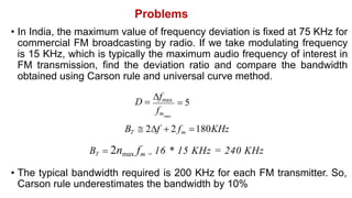
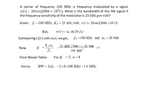
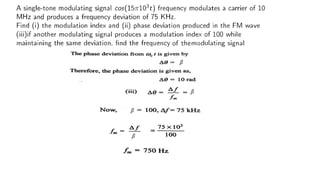
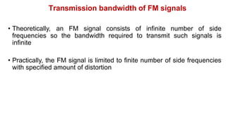
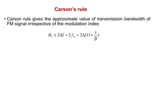
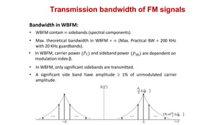
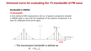
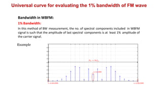
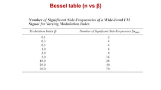
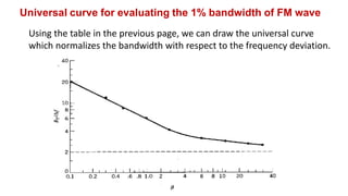
This document discusses bandwidth requirements for FM signals. It explains that theoretically an FM signal has infinite bandwidth due to its infinite number of sidebands, but practically the bandwidth is finite. Carson's rule provides an approximate value for transmission bandwidth regardless of modulation index. The 1% bandwidth method defines bandwidth as the number of spectral components where the last component's amplitude is at least 1% of the carrier amplitude. A universal curve relates bandwidth to frequency deviation ratio. Examples calculate deviation, index, bandwidth and power for various FM signals.

1. Transmission bandwidth of FM signals
• Theoretically, an FM signal consists of infinite number of side
frequencies so the bandwidth required to transmit such signals is
infinite
• Practically, the FM signal is limited to finite number of side frequencies
with specified amount of distortion

2. Carson’s rule
• Carson rule gives the approximate value of transmission bandwidth of
FM signal irrespective of the modulation index

B  2f  2 f  2f (1
1
)
T m

3. Transmission bandwidth of FM signals
Bandwidth in WBFM:
• WBFM contain  sidebands (spectral components).
• Max. theoretical bandwidth in WBFM =  (Max. Practical BW = 200 KHz
with 20 KHz guardbands).
• In WBFM, carrier power 𝑃C and sideband power
modulation index β.
𝑃SB are dependent on
• In WBFM, only significant sidebands are transmitted.
• A significant side band have amplitude  1% of unmodulated carrier
amplitude.
⋯
⋯
𝐴c
2
𝐽0 β
2
1% of Ac
𝐽0 β
𝑓c
—𝑓c
⋯
⋯
→ 𝑓
𝑆 𝑓

4. Universal curve for evaluating the 1% bandwidth of FM wave
•Carlson’s rule is simple to use, but it does not always provide a good estimate
of the bandwidth
•Define the transmission bandwidth as up to the band which is greater than
1% of the carrier amplitude.
• The transmission bandwidth is defined as
BT  2nmax fm
• nmax is the largest value of n that satisfies |Jn(β)>0.01|
• The value of n varies with the modulation index and can be determined
from the tabulated values of Bessel function

5. Universal curve for evaluating the 1% bandwidth of FM wave
Bandwidth in WBFM:
1% Bandwidth:
In this method of BW measurement, the no. of spectral components included
in WBFM signal is such that the amplitude of last spectral components is at
least 1% amplitude of the carrier signal.
⋯
⋯
𝐴c
2
𝐽0 β
2
1% of Ac
𝐽0 β
⋯
⋯
1% BW
• The transmission bandwidth is defined as
BT  2nmax fm

6. Universal curve for evaluating the 1% bandwidth of FM wave
Bandwidth in WBFM:
1% Bandwidth:
In this method of BW measurement, the no. of spectral components included in WBFM
signal is such that the amplitude of last spectral components is at least 1% amplitude of
the carrier signal.

7. Bessel table (n vs β)

8. Universal curve for evaluating the 1% bandwidth of FM wave
Using the table in the previous page, we can draw the universal curve
which normalizes the bandwidth with respect to the frequency deviation.

9. Deviation ratio and Percentage modulation
max
• Deviation ratio is defined as the ratio of the maximum frequency
deviation Δf to the maximum modulating signal frequency fm
D 
fmax
fm
• Percentage modulation is defined as the ratio of the actual frequency
deviation Δfactto the maximum frequency deviation Δfmax.
%modulation 
factual
fmax

10. Problems
• (a). Determine the peak frequency deviation and modulation index for
the FM modulator with a deviation sensitivity 5 KHz/V and a modulating
signal Vm(t)=2cos(2πХ2000t)
• (b). Determine the peak phase deviation and modulation index for the
FM modulator with a deviation sensitivity 2.5 rad/V and a modulating
signal Vm(t)=2cos(2πХ2000t)

11. Problems
• (a). Determine the peak frequency deviation and modulation index for
the FM modulator with a deviation sensitivity 5 KHz/V and a modulating
signal Vm(t)=2cos(2πХ2000t)
• (b). Determine the peak phase deviation for the FM modulator with a
deviation sensitivity 2.5 rad/V and a modulating signal
Vm(t)=2cos(2πХ2000t)
f  kf vm 10KHz
 
f
 5
fm
  kpvm  5rad

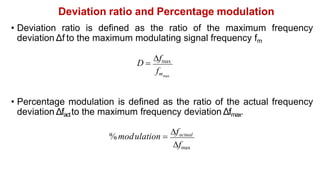
12. Problems
• An FM wave is represented by the equation
6 4
VFM (t) 10sin[810 t  6sin310 t]
• Calculate the modulating frequency, carrier frequency, modulation index,
frequency deviation

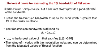
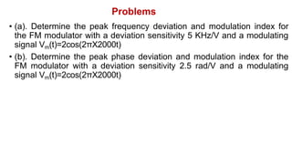
13. Problems
• An FM wave is represented by the equation
6 4
VFM (t) 10sin[810 t  6sin310 t]
• Calculate the modulating frequency, carrier frequency, modulation index,
frequency deviation
• Comparing with the standard FM equation
VFM (t)  Ac cos[2fct   sin 2fmt]
fm  4.77KHz
fc 1.27MHz
  6
f  28.62KHz

14. Problems
• A sinusoidal modulating waveform of amplitude 5 V and a frequency of 2
KHz is applied to FM generator, which has a frequency sensitivity of 40
Hz/volt. Calculate the frequency deviation, modulation index, and
bandwidth.

15. Problems
• A sinusoidal modulating waveform of amplitude 5 V and a frequency of 2
KHz is applied to FM generator, which has a frequency sensitivity of 40
Hz/volt. Calculate the frequency deviation, modulation index, and
bandwidth.
f  kf vm  200Hz
 
f
 0.1
fm
NBFM, BW  2 fm  4KHz

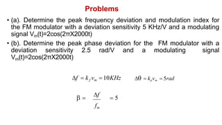
16. Problems
• An FM wave is represented by the equation
VFM (t)  20cos[8 106 t 9sin 2 103 t]
• Calculate the frequency deviation, bandwidth and power

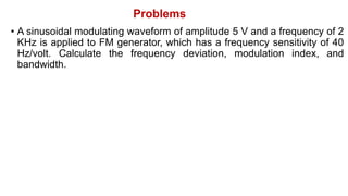
17. Problems
2R
• An FM wave is represented by the equation
VFM (t)  20cos[8 106 t 9sin 2 103 t]
• Calculate the frequency deviation, bandwidth and the average power
f  fm  9KHz
BW  2(f  fm )  20KHz
V 2
P  c
 200W

18. Problems
• In India, the maximum value of frequency deviation is fixed at 75 KHz for
commercial FM broadcasting by radio. If we take modulating frequency
is 15 KHz, which is typically the maximum audio frequency of interest in
FM transmission, find the deviation ratio and compare the bandwidth
obtained using Carson rule and universal curve method.

19. Problems
• In India, the maximum value of frequency deviation is fixed at 75 KHz for
commercial FM broadcasting by radio. If we take modulating frequency
is 15 KHz, which is typically the maximum audio frequency of interest in
FM transmission, find the deviation ratio and compare the bandwidth
obtained using Carson rule and universal curve method.
BT  2f  2 fm 180KHz
BT  2nmax fm = 16 * 15 KHz = 240 KHz
• The typical bandwidth required is 200 KHz for each FM transmitter. So,
Carson rule underestimates the bandwidth by 10%
 5
max
fm
D 
fmax

24. Bessel table (n vs β)