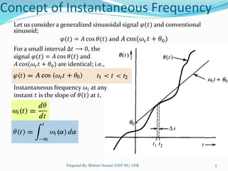
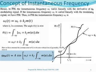
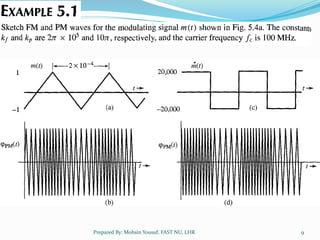
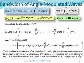
Angle modulation techniques were explored to help reduce static noise in communications. It was initially thought that frequency modulation (FM), where the carrier frequency varies proportionally to the message, could reduce bandwidth and thus noise. However, experimental results did not match expectations. The concept of instantaneous frequency was then developed to better understand angle-modulated signals. Different angle modulation techniques like frequency shift keying (FSK) and phase shift keying (PSK) were also introduced. Narrowband angle modulation can be achieved by ensuring the modulation index is small, while wideband modulation requires accounting for higher order terms in the modulation equation.

1. Angle (Exponential) Modulation

2. A Historical Note
2
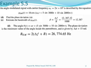
Prepared By: Mohsin Yousuf, FAST NU, LHR
 The constant search for techniques that lower static noise
in the communication lead to the exploring of angle
modulation.
 Noise power is proportional to modulated signal
bandwidth (sidebands) and it was thought that FM
(Frequency Modulation), where the carrier frequency is
varied in proportion to the message 𝑚(𝑡), thus
 𝐴 cos 𝜔𝑐(𝑡) becomes 𝐴 cos[𝜔𝑐 + 𝑘𝑚(𝑡)], where 𝑘 is an
arbitrary constant.
 The bandwidth for peak 𝑚𝑝 would be 2𝑘𝑚𝑝 centered at 𝜔𝑐.
So, by selecting a small 𝑘, we can reduce the bandwidth as
we please.
 However, the experimental results were not as expected.

3. Concept of Instantaneous Frequency
3
Prepared By: Mohsin Yousuf, FAST NU, LHR
Let us consider a generalized sinusoidal signal 𝜑(𝑡) and conventional
sinusoid;
𝜑(𝑡) = 𝐴 cos 𝜃(𝑡) and 𝐴 cos(𝜔𝑐𝑡 + 𝜃0)
For a small interval ∆𝑡 ⟶ 0, the
signal 𝜑(𝑡) = 𝐴 cos 𝜃(𝑡) and
𝐴 cos(𝜔𝑐𝑡 + 𝜃0) are identical; i.e.,
Instantaneous frequency 𝜔𝑖 at any
instant 𝑡 is the slope of 𝜃 𝑡 at 𝑡,

4. Concept of Instantaneous Frequency
4
Prepared By: Mohsin Yousuf, FAST NU, LHR

5. Concept of Instantaneous Frequency
5
Prepared By: Mohsin Yousuf, FAST NU, LHR

6. Generalized Concept of Angle Modulation
6
Prepared By: Mohsin Yousuf, FAST NU, LHR

7. Generalized Concept of Angle Modulation
7
Prepared By: Mohsin Yousuf, FAST NU, LHR

8. Generalized Concept of Angle Modulation
8
Prepared By: Mohsin Yousuf, FAST NU, LHR

9. Prepared By: Mohsin Yousuf, FAST NU, LHR 9

10. Prepared By: Mohsin Yousuf, FAST NU, LHR 10
FSK PSK

11. Prepared By: Mohsin Yousuf, FAST NU, LHR 11
PSK

12. Prepared By: Mohsin Yousuf, FAST NU, LHR 12
PSK
When 𝑚(𝑡) is a digital signal, 𝜑𝑃𝑀(𝑡) shows a phase discontinuity where 𝑚 𝑡 has a jump
discontinuity. In such cases 𝑘𝑝𝑚 𝑡 must be restricted to a range (−𝜋, 𝜋) in order to avoid
ambiguity in demodulation. Because a phase 𝜑0 + 2𝑛𝜋 is indistinguishable from the phase
𝜑0 in the demodulator. In addition, 𝑘𝑝 should be small enough to restrict phase change.

13. Prepared By: Mohsin Yousuf, FAST NU, LHR 13
PSK
FSK

14. Bandwidth of Angle-Modulated Waves
Prepared By: Mohsin Yousuf, FAST NU, LHR 14

15. Bandwidth of Angle-Modulated Waves
Prepared By: Mohsin Yousuf, FAST NU, LHR 15

16. Narrow-Band Angle-Modulation
Prepared By: Mohsin Yousuf, FAST NU, LHR 16

17. Narrow-Band PM & FM wave generation
Prepared By: Mohsin Yousuf, FAST NU, LHR 17

18. Wide-band FM (WBFM): The Fallacy Exposed
Prepared By: Mohsin Yousuf, FAST NU, LHR 18
If 𝑘𝑓𝑎(𝑡) ≪ 1 is not satisfied, we can not ignore the higher-order terms.

19. Wide-band FM (WBFM): The Fallacy Exposed
Prepared By: Mohsin Yousuf, FAST NU, LHR 19
Max Freq: 𝜔𝑐 + 𝑘𝑓𝑚𝑝 + 4𝜋𝐵
Min Freq: 𝜔𝑐 − 𝑘𝑓𝑚𝑝 − 4𝜋𝐵
Spectrum BW: 2𝑘𝑓𝑚𝑝 + 8𝜋𝐵

20. Wide-band FM (WBFM): The Fallacy Exposed
Prepared By: Mohsin Yousuf, FAST NU, LHR 20
Spectrum BW: 2𝑘𝑓𝑚𝑝 + 8𝜋𝐵
The deviation of the carrier frequency is ∆𝜔 = ±𝑘𝑓𝑚𝑝
Carrier frequency deviation in Hertz is ∆𝑓 =
𝑘𝑓𝑚𝑝
2𝜋
The estimated bandwidth (in Hz) can be expressed as:
𝐵𝐹𝑀 =
1
2𝜋
2𝑘𝑓𝑚𝑝 + 8𝜋𝐵
= 2 ∆𝑓 + 2𝐵
Carson′
s Rule: 2 ∆𝑓 + 𝐵
= 2
𝑘𝑓𝑚𝑝
2𝜋
+ 𝐵
Deviation Ratio: 𝛽 =
∆𝑓
𝐵
𝐵𝐹𝑀 = 2𝐵(𝛽 + 1)

21. Wide-band PM (WBPM)
Prepared By: Mohsin Yousuf, FAST NU, LHR 21
The deviation of the carrier
frequency is ∆𝜔 = 𝑘𝑝𝑚′𝑝
Carrier frequency deviation in
Hertz is ∆𝑓 =
𝑘𝑝𝑚′𝑝
2𝜋
The estimated bandwidth (in
Hz) can be expressed as:
𝐵𝑃𝑀 = 2 ∆𝑓 + 𝐵
= 2
𝑘𝑝𝑚′
𝑝
2𝜋
+ 𝐵

22. Verification of FM Bandwidth Relationship
Prepared By: Mohsin Yousuf, FAST NU, LHR 22

23. Example 5.3
Prepared By: Mohsin Yousuf, FAST NU, LHR 23
a) Estimate 𝐵𝐹𝑀 and 𝐵𝑃𝑀 for the modulating signal 𝑚 𝑡 in Fig 5.4 (a) for 𝑘𝑓 = 2𝜋 × 105
and 𝑘𝑝 = 5𝜋.
b) Repeat the problem if 𝑚(𝑡) is doubled.

24. Example 5.3 (Contd.)
Prepared By: Mohsin Yousuf, FAST NU, LHR 24
a) Estimate 𝐵𝐹𝑀 and 𝐵𝑃𝑀 for the modulating signal 𝑚 𝑡 in Fig 5.4 (a) for 𝑘𝑓 = 2𝜋 × 105
and 𝑘𝑝 = 5𝜋.
b) Repeat the problem if 𝑚(𝑡) is doubled.

25. Example 5.3 (Contd.)
Prepared By: Mohsin Yousuf, FAST NU, LHR 25
a) Estimate 𝐵𝐹𝑀 and 𝐵𝑃𝑀 for the modulating signal 𝑚 𝑡 in Fig 5.4 (a) for 𝑘𝑓 = 2𝜋 × 105
and 𝑘𝑝 = 5𝜋.
b) Repeat the problem if 𝑚(𝑡) is doubled.

26. Example 5.3 (Contd.)
Prepared By: Mohsin Yousuf, FAST NU, LHR 26
a) Estimate 𝐵𝐹𝑀 and 𝐵𝑃𝑀 for the modulating signal 𝑚 𝑡 in Fig 5.4 (a) for 𝑘𝑓 = 2𝜋 × 105
and 𝑘𝑝 = 5𝜋.
b) Repeat the problem if 𝑚(𝑡) is doubled.
2
−2

27. Example 5.3 (Contd.)
Prepared By: Mohsin Yousuf, FAST NU, LHR 27
a) Estimate 𝐵𝐹𝑀 and 𝐵𝑃𝑀 for the modulating signal 𝑚 𝑡 in Fig 5.4 (a) for 𝑘𝑓 = 2𝜋 × 105
and 𝑘𝑝 = 5𝜋.
b) Repeat the problem if 𝑚(𝑡) is doubled.
2
−2

28. Example 5.3 (Contd.)
Prepared By: Mohsin Yousuf, FAST NU, LHR 28
4

29. Example 5.3 (Contd.)
Prepared By: Mohsin Yousuf, FAST NU, LHR 29
4

30. Example 5.5
Prepared By: Mohsin Yousuf, FAST NU, LHR 30

31. Example 5.5
Prepared By: Mohsin Yousuf, FAST NU, LHR 31