The document defines the operators curl and divergence for vector fields. Curl is defined as the cross product of del (the gradient operator) with the vector field and results in another vector. Divergence is defined as the dot product of del with the vector field and results in a scalar. Several examples of computing curl and divergence are worked out. Green's theorem, which relates line integrals of vector fields to surface integrals of curl and divergence, is also discussed.
In this presentation we will learn Del operator, Gradient of scalar function , Directional Derivative, Divergence of vector function, Curl of a vector function and after that solved some example related to above.
Gradient in math
Directional derivative in math
Divergence in math
Curl in math
Gradient , Directional Derivative , Divergence , Curl in mathematics
Gradient , Directional Derivative , Divergence , Curl in math
Gradient , Directional Derivative , Divergence , Curl
The cross product is an important operation, taking two three-dimensional vectors and producing a three-dimensional vector. It's not a product in the commutative, associative, sense, but it does produce a vector which is perpendicular to the two crossed vectors and whose length is the area of the parallelogram spanned by the them. The direction is chosen again to follow the right-hand rule.
The cross product is an important operation, taking two three-dimensional vectors and producing a three-dimensional vector. It's not a product in the commutative, associative, sense, but it does produce a vector which is perpendicular to the two crossed vectors and whose length is the area of the parallelogram spanned by the them. The direction is chosen again to follow the right-hand rule.
I am Britney. I am a Differential Equations Assignment Solver at mathhomeworksolver.com. I hold a Master's in Mathematics, from London, UK. I have been helping students with their assignments for the past 10 years. I solved assignments related to Differential Equations Assignment.
Visit mathhomeworksolver.com or email support@mathhomeworksolver.com. You can also call on +1 678 648 4277 for any assistance with Differential Equations Assignment.
I am Steven M. I am a Maths Assignment Expert at mathsassignmenthelp.com. I hold a Master's in Mathematics from Ryerson University. I have been helping students with their assignments for the past 10 years. I solve assignments related to Maths.
Visit mathsassignmenthelp.com or email info@mathsassignmenthelp.com.
You can also call +1 678 648 4277 for any assistance with Maths Assignments.
International Journal of Engineering Research and Applications (IJERA) is an open access online peer reviewed international journal that publishes research and review articles in the fields of Computer Science, Neural Networks, Electrical Engineering, Software Engineering, Information Technology, Mechanical Engineering, Chemical Engineering, Plastic Engineering, Food Technology, Textile Engineering, Nano Technology & science, Power Electronics, Electronics & Communication Engineering, Computational mathematics, Image processing, Civil Engineering, Structural Engineering, Environmental Engineering, VLSI Testing & Low Power VLSI Design etc.
Integral Calculus. - Differential Calculus - Integration as an Inverse Process of Differentiation - Methods of Integration - Integration using trigonometric identities - Integrals of Some Particular Functions - rational function - partial fraction - Integration by partial fractions - standard integrals - First and second fundamental theorem of integral calculus
A tutorial on the Frobenious Theorem, one of the most important results in differential geometry, with emphasis in its use in nonlinear control theory. All results are accompanied by proofs, but for a more thorough and detailed presentation refer to the book of A. Isidori.
Quality defects in TMT Bars, Possible causes and Potential Solutions.PrashantGoswami42
Maintaining high-quality standards in the production of TMT bars is crucial for ensuring structural integrity in construction. Addressing common defects through careful monitoring, standardized processes, and advanced technology can significantly improve the quality of TMT bars. Continuous training and adherence to quality control measures will also play a pivotal role in minimizing these defects.
Courier management system project report.pdfKamal Acharya
It is now-a-days very important for the people to send or receive articles like imported furniture, electronic items, gifts, business goods and the like. People depend vastly on different transport systems which mostly use the manual way of receiving and delivering the articles. There is no way to track the articles till they are received and there is no way to let the customer know what happened in transit, once he booked some articles. In such a situation, we need a system which completely computerizes the cargo activities including time to time tracking of the articles sent. This need is fulfilled by Courier Management System software which is online software for the cargo management people that enables them to receive the goods from a source and send them to a required destination and track their status from time to time.
Overview of the fundamental roles in Hydropower generation and the components involved in wider Electrical Engineering.
This paper presents the design and construction of hydroelectric dams from the hydrologist’s survey of the valley before construction, all aspects and involved disciplines, fluid dynamics, structural engineering, generation and mains frequency regulation to the very transmission of power through the network in the United Kingdom.
Author: Robbie Edward Sayers
Collaborators and co editors: Charlie Sims and Connor Healey.
(C) 2024 Robbie E. Sayers
Final project report on grocery store management system..pdfKamal Acharya
In today’s fast-changing business environment, it’s extremely important to be able to respond to client needs in the most effective and timely manner. If your customers wish to see your business online and have instant access to your products or services.
Online Grocery Store is an e-commerce website, which retails various grocery products. This project allows viewing various products available enables registered users to purchase desired products instantly using Paytm, UPI payment processor (Instant Pay) and also can place order by using Cash on Delivery (Pay Later) option. This project provides an easy access to Administrators and Managers to view orders placed using Pay Later and Instant Pay options.
In order to develop an e-commerce website, a number of Technologies must be studied and understood. These include multi-tiered architecture, server and client-side scripting techniques, implementation technologies, programming language (such as PHP, HTML, CSS, JavaScript) and MySQL relational databases. This is a project with the objective to develop a basic website where a consumer is provided with a shopping cart website and also to know about the technologies used to develop such a website.
This document will discuss each of the underlying technologies to create and implement an e- commerce website.
Welcome to WIPAC Monthly the magazine brought to you by the LinkedIn Group Water Industry Process Automation & Control.
In this month's edition, along with this month's industry news to celebrate the 13 years since the group was created we have articles including
A case study of the used of Advanced Process Control at the Wastewater Treatment works at Lleida in Spain
A look back on an article on smart wastewater networks in order to see how the industry has measured up in the interim around the adoption of Digital Transformation in the Water Industry.
Industrial Training at Shahjalal Fertilizer Company Limited (SFCL)MdTanvirMahtab2
This presentation is about the working procedure of Shahjalal Fertilizer Company Limited (SFCL). A Govt. owned Company of Bangladesh Chemical Industries Corporation under Ministry of Industries.
Explore the innovative world of trenchless pipe repair with our comprehensive guide, "The Benefits and Techniques of Trenchless Pipe Repair." This document delves into the modern methods of repairing underground pipes without the need for extensive excavation, highlighting the numerous advantages and the latest techniques used in the industry.
Learn about the cost savings, reduced environmental impact, and minimal disruption associated with trenchless technology. Discover detailed explanations of popular techniques such as pipe bursting, cured-in-place pipe (CIPP) lining, and directional drilling. Understand how these methods can be applied to various types of infrastructure, from residential plumbing to large-scale municipal systems.
Ideal for homeowners, contractors, engineers, and anyone interested in modern plumbing solutions, this guide provides valuable insights into why trenchless pipe repair is becoming the preferred choice for pipe rehabilitation. Stay informed about the latest advancements and best practices in the field.
Saudi Arabia stands as a titan in the global energy landscape, renowned for its abundant oil and gas resources. It's the largest exporter of petroleum and holds some of the world's most significant reserves. Let's delve into the top 10 oil and gas projects shaping Saudi Arabia's energy future in 2024.
Top 10 Oil and Gas Projects in Saudi Arabia 2024.pdf
13 05-curl-and-divergence
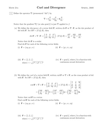
1. Math 21a Curl and Divergence Spring, 2009
1 Define the operator (pronounced “del”) by
= i
∂
∂x
+ j
∂
∂y
+ k
∂
∂z
.
Notice that the gradient f (or also grad f) is just applied to f.
(a) We define the divergence of a vector field F, written div F or · F, as the dot product of
del with F. So if F = P, Q, R , then
div F = · F =
∂
∂x
,
∂
∂y
,
∂
∂z
· P, Q, R =
∂P
∂x
+
∂Q
∂y
+
∂R
∂z
.
Notice that div F is a scalar.
Find div F for each of the following vector fields:
(i) F = xy, yz, xz (ii) F = yz, xz, xy
(iii) F = x
r
, y
r
, z
r
where r = x2 + y2 + z2
(iv) F = grad f, where f is a function with
continuous second derivatives
(b) We define the curl of a vector field F, written curl F or × F, as the cross product of del
with F. So if F = P, Q, R , then
curl F = × F =
∂
∂x
,
∂
∂y
,
∂
∂z
× P, Q, R =
i j k
∂
∂x
∂
∂y
∂
∂z
P Q R
=
∂R
∂y
−
∂Q
∂z
i +
∂P
∂z
−
∂R
∂x
j +
∂Q
∂x
−
∂P
∂y
k.
Notice that curl F is a vector.
Find curl F for each of the following vector fields:
(i) F = xy, yz, xz (ii) F = yz, xz, xy
(iii) F = x
r
, y
r
, z
r
where r = x2 + y2 + z2
(iv) F = grad f, where f is a function with
continuous second derivatives
2. 2 Check the appropriate box (“Vector”, “Scalar”, or “Nonsense”) for each quantity.
Quantity Vector Scalar Nonsense
curl( f)
· ( × F)
div(curl f)
curl(curl F)
( · F)
Quantity Vector Scalar Nonsense
curl(curl f)
grad(div f)
div(grad F)
· ( f)
div(div F)
3 (a) Suppose we have a vector P, Q that we extend to a vector in space: F = P(x, y), Q(x, y), 0 .
Find curl F.
(b) When is the vector field F in part (a) conservative? Use the curl in your answer.
(c) If F = f = fx, fy, fz is conservative, then is curl F = 0? (See Problem 1(b)(iv).)
In fact, we can identify conservative vector fields with the curl:
Theorem: Let F be a vector field defined on all of R3
. If the component
functions of F all have continuous derivatives and curl F = 0, then F is a
conservative vector field.
4 Show that, if F is a vector field on R3
with components that have continuous second-order
derivatives, then div curl F = 0. (This is less useful for us right now than curl grad f = 0, but
it’s not a difficult computation.)
3. 5 We can re-write Green’s theorem in vector form (we get the formula on the left, below). The
formula on the right can be thought of as a version of Green’s theorem that uses the normal
component rather than the tangential component:
C
F · dr =
D
(curl F) · k dA and
C
F · n ds =
D
div F(x, y) dA.
(If r = x(t), y(t) , then n = y (t),−x (t)
| y (t),−x (t) |
is the outward unit normal.) For each of the following
vector fields F and paths C, compute the integrals above using these vector forms of Green’s
theorem:
(a) F = −y, x and C is the unit circle, positively oriented.
(b) F = 2x, 2y and C is the unit square (with corners at (0, 0), (1, 0), (1, 1) and (0, 1)),
positively oriented.
(While we’ll never really look at the normal version of Green’s theorem again, one of our
big integral theorems next week can be thought of as a higher-dimensional version of it.)
6 Here are sketches of a few vector fields F = P(x, y), Q(x, y), 0 (they’re drawn in the plane, but
they’re defined in all of space). Can you tell which one has zero curl? Zero divergence?
−4 4
................................................................................................................................................................................................................................................................................................................................................. ...................
−4
4
.................................................................................................................................................................................................................................................................................................................................................
...................
x
y
.............................................................. ..........
........................................................ ..........
...................................................
..........
................................................
..........
...............................................
..........
................................................
..........
...................................................
..........
........................................................
..........
..............................................................
..........
........................................................ ..........
................................................. ..........
.....................................................
.......................................
..........
......................................
..........
.......................................
..........
...........................................
..........
.................................................
..........
........................................................
..........
................................................... ..........
........................................... ..........
.................................... ..........
...............................
..........
.............................
..........
...............................
..........
....................................
..........
...........................................
..........
.............................................................
................................................ ..........
....................................... ..........
............................... ..........
....................... ..........
....................
..........
.......................
..........
.........................................
.................................................
..........................................................
............................................... ..........
...................................... ..........
............................. ..........
.................... ..........
•
..............................
.......................................
................................................
.........................................................
................................................ ..........
....................................... ..........
.........................................
.......................
..........
....................
..........
.................................
.........................................
.................................................
..........................................................
.............................................................
...........................................
..........
....................................
..........
...............................
..........
.............................
..........
...............................
..........
..............................................
.....................................................
.............................................................
........................................................
..........
.................................................
..........
...........................................
..........
.......................................
..........
......................................
..........
.......................................
..........
.....................................................
...........................................................
..................................................................
..............................................................
..................................................................
.............................................................
..........
................................................
..........
...............................................
..........
................................................
..........
...................................................
..........
..................................................................
........................................................................
F = −y, x, 0
−4 4
................................................................................................................................................................................................................................................................................................................................................. ...................
−4
4
.................................................................................................................................................................................................................................................................................................................................................
...................
x
y
.........................................
..........
......................................
..........
...................................
..........
.................................
..........
................................
..........
.................................
..........
...................................
..........
...................................... ..........
......................................... ..........
......................................
..........
.................................
..........
..............................
..........
............................
..........
...........................
..........
............................
..........
........................................
................................. ..........
...................................... ..........
.............................................
..............................
..........
..........................
..........
.......................
..........
.....................
..........
.......................
..........
.......................... ..........
.............................. ..........
................................... ..........
...........................................
......................................
.................................
..................
..........
................
..........
.................. ..........
....................... ..........
............................ ..........
................................. ..........
..........................................
.....................................
...............................
..........................
•
................ ..........
..................... ..........
........................... ..........
................................ ..........
...........................................
......................................
.................................
............................
................
..........
..................
..........
.................................
............................ ..........
................................. ..........
.............................................
........................................
....................................
.......................
..........
.....................
..........
.......................
..........
..........................
..........
..............................
..........
.............................................
................................................
...........................................
........................................
............................
..........
...........................
..........
............................
..........
..............................
..........
.................................
..........
......................................
..........
...................................................
................................................
...................................
..........
.................................
..........
................................
..........
.................................
..........
...................................
..........
......................................
..........
.........................................
..........
F = y, x, 0
−4 4
................................................................................................................................................................................................................................................................................................................................................. ...................
−4
4
.................................................................................................................................................................................................................................................................................................................................................
...................
x
y
........................................................................
..........
.................................................................
..........
.....................................................................
.................................................................
................................................................
.................................................................
.....................................................................
...........................................................................
..................................................................................
.................................................................
..........
........................................................
..........
..................................................
..........
.......................................................
.....................................................
.......................................................
............................................................
..................................................................
...........................................................................
...........................................................
..........
..................................................
..........
.........................................
..........
.............................................
..........................................
.............................................
...................................................
............................................................
...........................................................
..........
.......................................................
..........
.............................................
..........
...................................
..........
..........................
..........
...............................
....................................
...................................
..........
.............................................
..........
.......................................................
..........
......................................................
..........
...........................................
..........
................................
..........
.....................
..........
•
.....................
..........
................................
..........
...........................................
..........
......................................................
..........
.......................................................
..........
.............................................
..........
...................................
..........
.......................... ..........
..................... ..........
..........................
..........
...................................
..........
.............................................
..........
.......................................................
..........
...........................................................
..........
............................................................
......................................... ..........
................................... ..........
................................ ..........
.............................................
.........................................
..........
..................................................
..........
...........................................................
..........
................................................................. ..........
........................................................ ..........
.................................................. ..........
............................................. ..........
........................................... ..........
............................................. ..........
..................................................
..........
........................................................
..........
.................................................................
..........
........................................................................ ..........
................................................................. ..........
........................................................... ..........
....................................................... ..........
...................................................... ..........
....................................................... ..........
.....................................................................
.................................................................
..........
........................................................................
..........
F = 2x, 2y, 0
4. Curl and Divergence – Answers and Solutions
1 (a) (i) div F = x + y + z
(ii) div F = 0
(iii) div F = y2+z2
r3 + x2+z2
r3 + x2+y2
r3 = 2(x2+y2+z2)
r3 = 2
r
(iv) div F = div(grad f) = fxx + fyy + fzz. This is the Laplace operator applied to f.
(b) (i) curl F = −y, −z, −x
(ii) curl F = 0
(iii) curl F = 0
(iv) curl F = curl(grad f) = 0.
Two quick comments:
• Notice that the vector from part (ii) is actually an example of this, since F =
grad(xyz) = yz, xz, xy . The vector for part (iii) is F = grad( x2 + y2 + z2), so
it is another example as well.
• We’ll see later on in this worksheet that curl F = 0 precisely when F = grad f (when
we make some continuity assumptions about the derivatives of the components of
F.
2 Here are some answers, although half are blank as they match questions from the homework:
Quantity Vector Scalar Nonsense
curl( f) x
· ( × F) x
div(curl f) x
curl(curl F)
( · F)
Quantity Vector Scalar Nonsense
curl(curl f) x
grad(div f)
div(grad F) x
· ( f)
div(div F)
3 (a) curl F = 0, 0, ∂Q
∂x
− ∂P
∂y
= 0, 0, Qx − Py
(b) A planar vector field F = P, Q is conservative when Qx − Py = 0. This means there’s a
function f(x, y) with P = fx and Q = fy. We also get fz = 0 since f is a function of only
x and y, so F = P(x, y), Q(x, y), 0 is conservative under this same condition. From part
(a), this means that F is conservative when curl F = 0.
(c) Yep, we’ve already seen that curl grad f = 0.
4 Here’s a quick detailed computation:
div curl F = div ( × P, Q, R )
= ·
∂R
∂y
−
∂Q
∂z
i +
∂P
∂z
−
∂R
∂x
j +
∂Q
∂x
−
∂P
∂y
k
=
∂
∂x
∂R
∂y
−
∂Q
∂z
+
∂
∂y
∂P
∂z
−
∂R
∂x
+
∂
∂z
∂Q
∂x
−
∂P
∂y
=
∂2
R
∂x ∂y
−
∂2
Q
∂x ∂z
+
∂2
P
∂y ∂z
−
∂2
R
∂y ∂x
+
∂2
Q
∂z ∂x
−
∂2
P
∂z ∂y
= (Ryx − Qzx) + (Pzy − Rxy) + (Qxz − Pyz) .
5. 5 (a) We do this both ways, of course. First let’s parameterize C by r(t) = x, y = cos(t), sin(t) ,
so dx = − sin(t) dt and dy = cos(t) dt. Thus
C
F · dr =
2π
0
− sin(t), cos(t) · − sin(t), cos(t) dt =
2π
0
1 dt = 2π.
The double integral is also straightforward: writing F = −y, x, 0 as a vector field in space,
we get curl F = 0, 0, 2 . Thus, since k = 0, 0, 1 , we get
D
(curl F) · k dA =
D
2 dA = 2 · Area(D) = 2π.
The normal component version requires us to have a unit outward-pointing normal n. For
the unit circle, the unit normal at the point (x, y) is simply n = x, y . (One way to see
this is to parameterize the circle as r(t) = x(t), y(t) = cos(t), sin(t) , so by our formula n
is the unit vector in the direction y (t), −x (t) = cos(t), sin(t) . But this is a unit vector
already, and in fact it is the vector x, y .) Thus F · n = −y, x · x, y = 0, so the line
integral is zero. Note also that div F = ∂
∂x
(−y) + ∂
∂y
(x) = 0, so the double integral is also
zero.
(b) Again we do this both ways. We’ll parameterize C in four parts (all with 0 ≤ t ≤ 1):
C1 : r(t) = x, y = t, 0 C2 : r(t) = x, y = 1, t
C3 : r(t) = x, y = 1 − t, 1 C4 : r(t) = x, y = 0, 1 − t
From this we get four integrals:
C1
F · dr =
C1
2x, 2y · dx, dy =
1
0
2t, 0 · dt, 0 =
1
0
2t dt = 1
C2
F · dr =
C2
2x, 2y · dx, dy =
1
0
2, 2t · 0, dt =
1
0
2t dt = 1
C3
F · dr =
C3
2x, 2y · dx, dy =
1
0
2(1 − t), 2 · −dt, 0 =
1
0
2(t − 1) dt = −1
C4
F · dr =
C4
2x, 2y · dx, dy =
1
0
0, 2(1 − t) · 0, −dt =
1
0
2(t − 1) dt = −1.
Thus
C
F · dr =
C1
+
C2
+
C3
+
C4
= 1 + 1 − 1 − 1 = 0.
The double integral is considerably easier: writing F = 2x, 2y, 0 as a vector field in space,
we compute curl F = 0, so the integrand in the double integral is zero. Thus the double
integral is zero as well.
The normal component version requires us to have a unit outward-pointing normal n. These
are simple to find for each component (using the above parameterization):
C1 : n = −j = 0, −1 C2 : n = i = 1, 0 ,
C3 : n = j = 0, 1 , C4 : n = −i = −1, 0 .
6. Thus the integrals are all (note that ds = dt in each case)
C1
F · n ds =
1
0
2t, 0 · 0, −1 dt = 0
C2
F · n ds =
1
0
2, 2t · 1, 0 dt =
1
0
2 dt = 2
C3
F · n ds =
1
0
2(1 − t), 2 · 0, 1 dt =
1
0
2 dt = 2
C4
F · n ds =
1
0
0, 2(1 − t) · −1, 0 = 0.
Thus
C
F · n ds =
C1
+
C2
+
C3
+
C4
= 0 + 2 + 2 + 0 = 4.
The double integral is again much simpler: we compute div F = 2 + 2 = 4, so the double
integral is just 4 times the area of the square. Thus the double integral has value 4 as well.
6 The idea here is that we can do this two ways: first, we can compute the curl and divergence of
the given vector fields:
(a) div F = 0
curl F = 0, 0, 2
(b) div F = 0
curl F = 0
(c) div F = 4
curl F = 0
Thus we see that the first vector field is the only one with a non-zero curl, and that the last
vector field is similarly the only one with a non-zero divergence.
Here’s a way to see this from the graph. We’ll use the two Green’s theorems from the previous
problem:
C
F · T ds =
D
(curl F) · k dA
C
F · n ds =
D
div F dA.
(Here we’ve written the first one slightly differently, but it’s the same. Since dr = r (t) dt and
T = r (t)
|r (t)|
and ds = |r (t)| dt, we get dr = T ds.)
Let’s start with the curl and the first of Green’s theorems. Let’s integrate around a small circle
C centered at the origin. We’ll choose it so small that curl F is essentially constant on the tiny
little disk D bounded by C. By this argument, the double integral is roughly
D
(curl F) · k dA ≈
D
(curl F(0, 0, 0)) · k dA = (curl F(0, 0, 0)) · k · Area(D).
On the other hand, the line integral is the integral of F · T. This is the tangential component of
F, and in particular
F · T 0 means F and T are mostly in the same direction,
F · T 0 means F and T are mostly in opposing directions, and
7. In the case of the first sketch, it’s clear that F is mostly parallel to the tangent vector to the
small circle C, so F · T 0. Thus C
F · T ds 0, so by Green’s theorem,
(curl F(0, 0, 0)) · k 0.
The moral: the curl of F is non-zero means that there is some kind of rotation in the vector
field. We’ll see much more of this later.
We could do something similar with the divergence. Let’s cut straight to the chase: the (outward-
pointing) normal n produces a positive divergence at the origin. This gives us what we call a
source (when div F 0) at the origin; if the vector fields were pointing in we’d get a sink (and
div F 0).