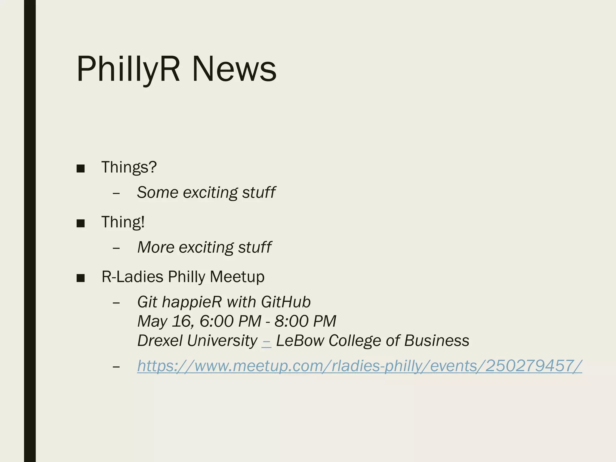
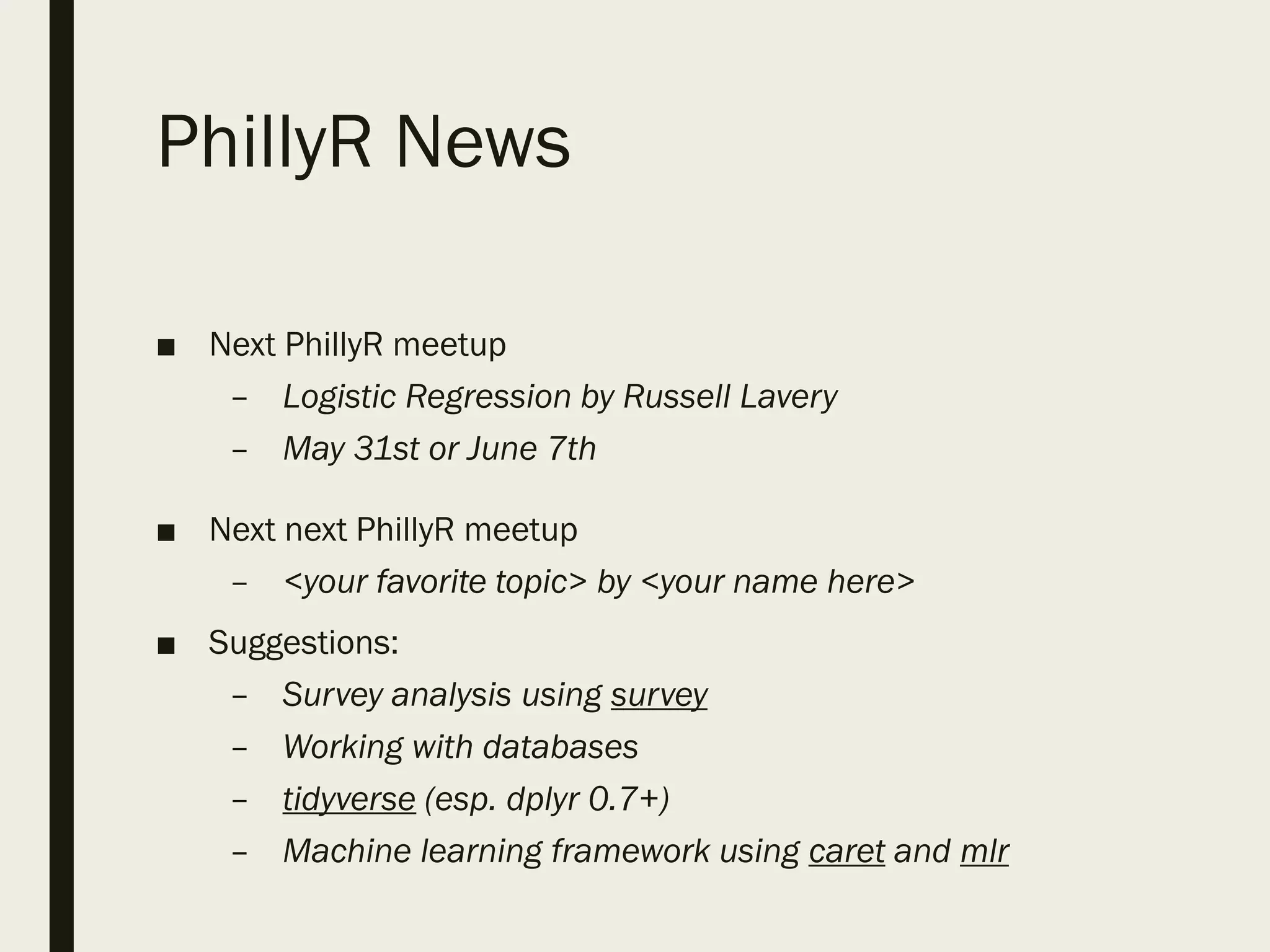
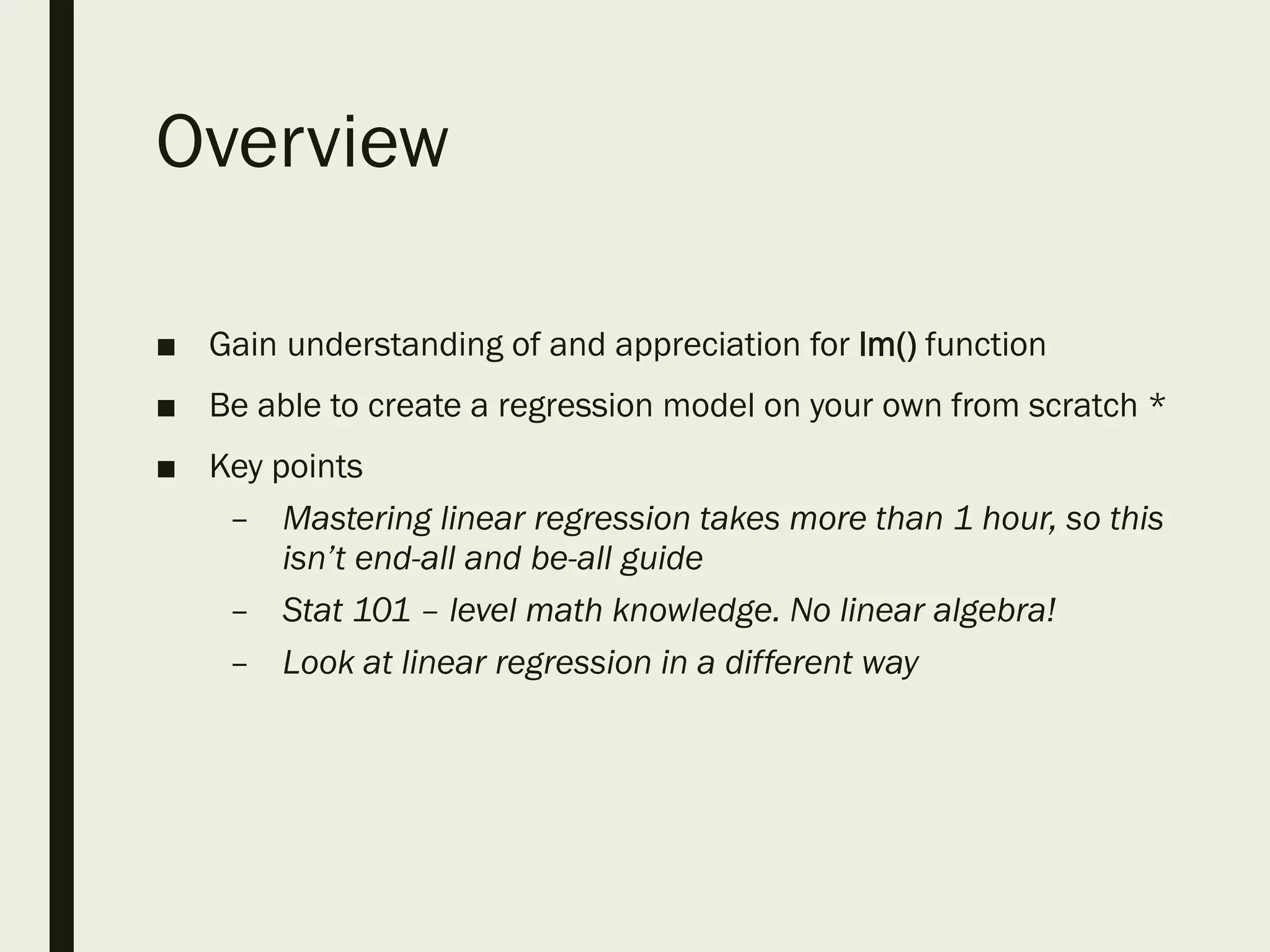
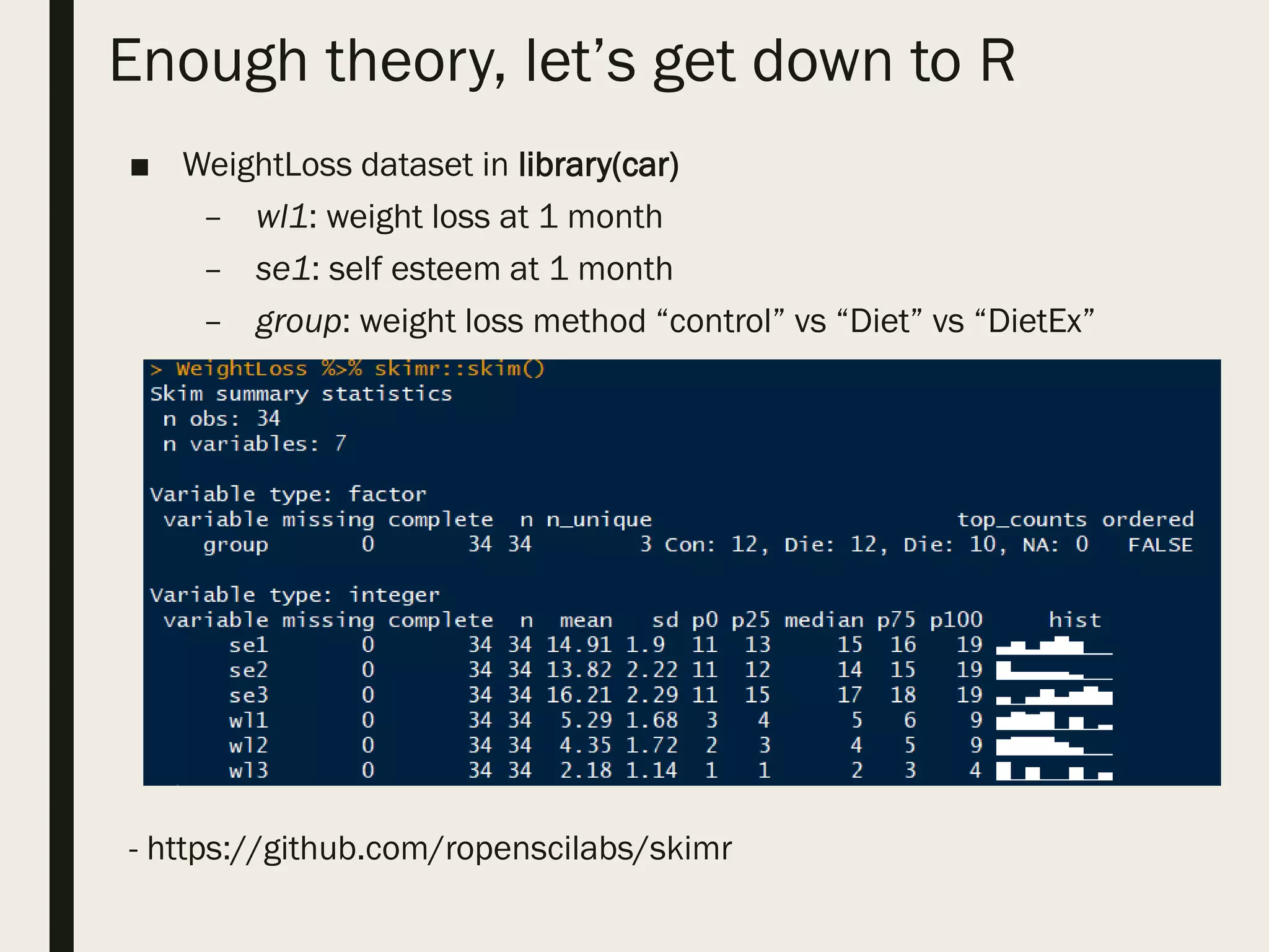
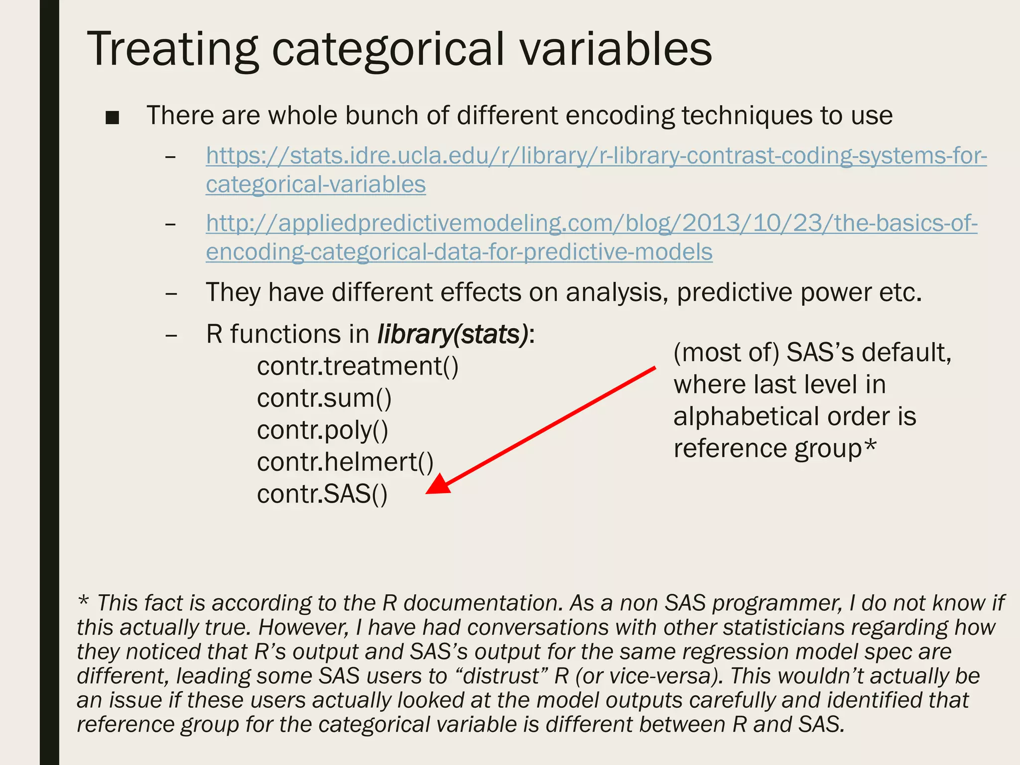
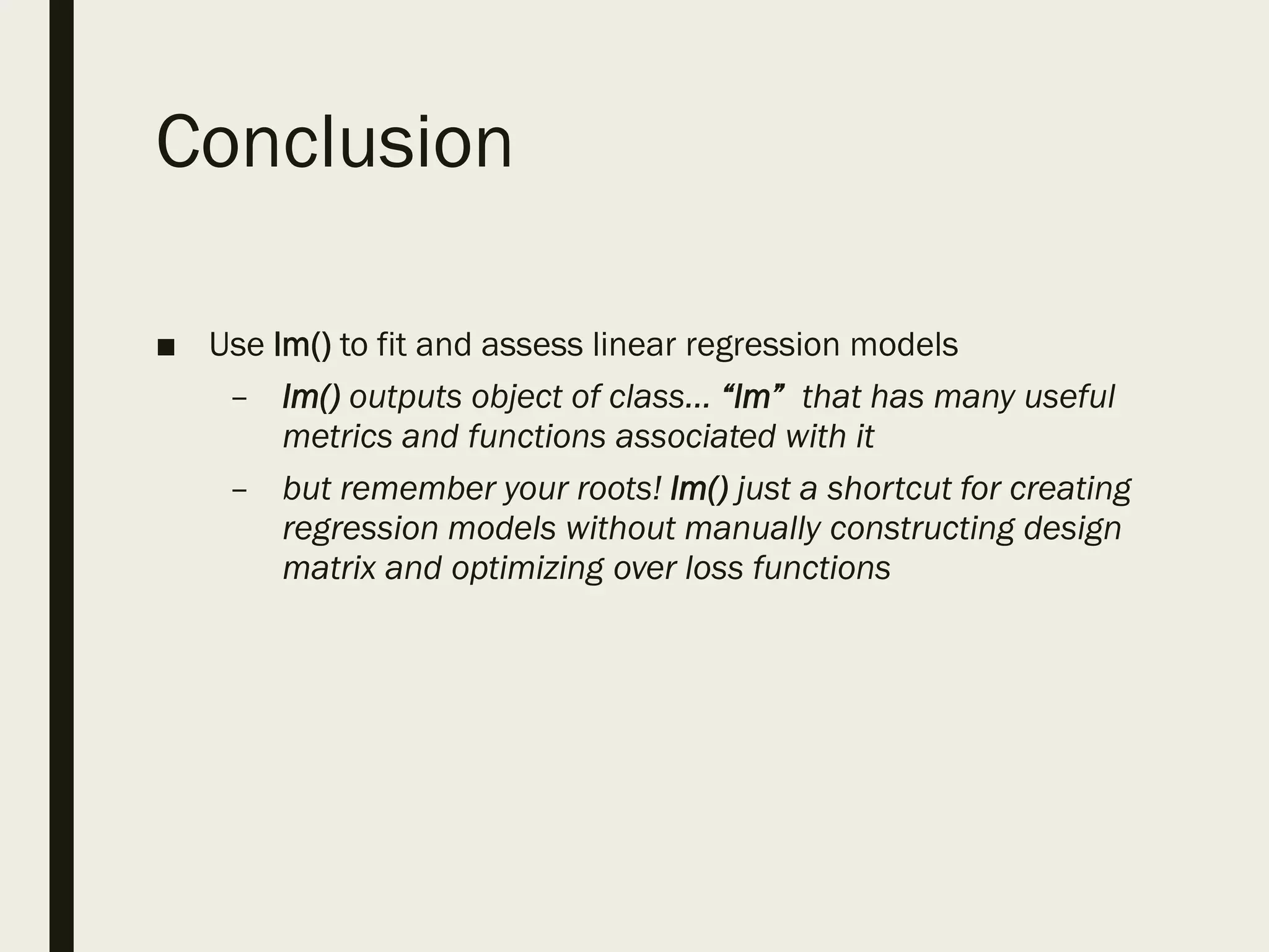
This document summarizes a meetup for the PhillyR R User Group on May 3, 2018. It provides an overview of the meetup agenda including a presentation on linear regression and time for Q&A. It also announces upcoming events, including a meetup on logistic regression on May 31 or June 7 and encourages suggestions for future presentation topics.
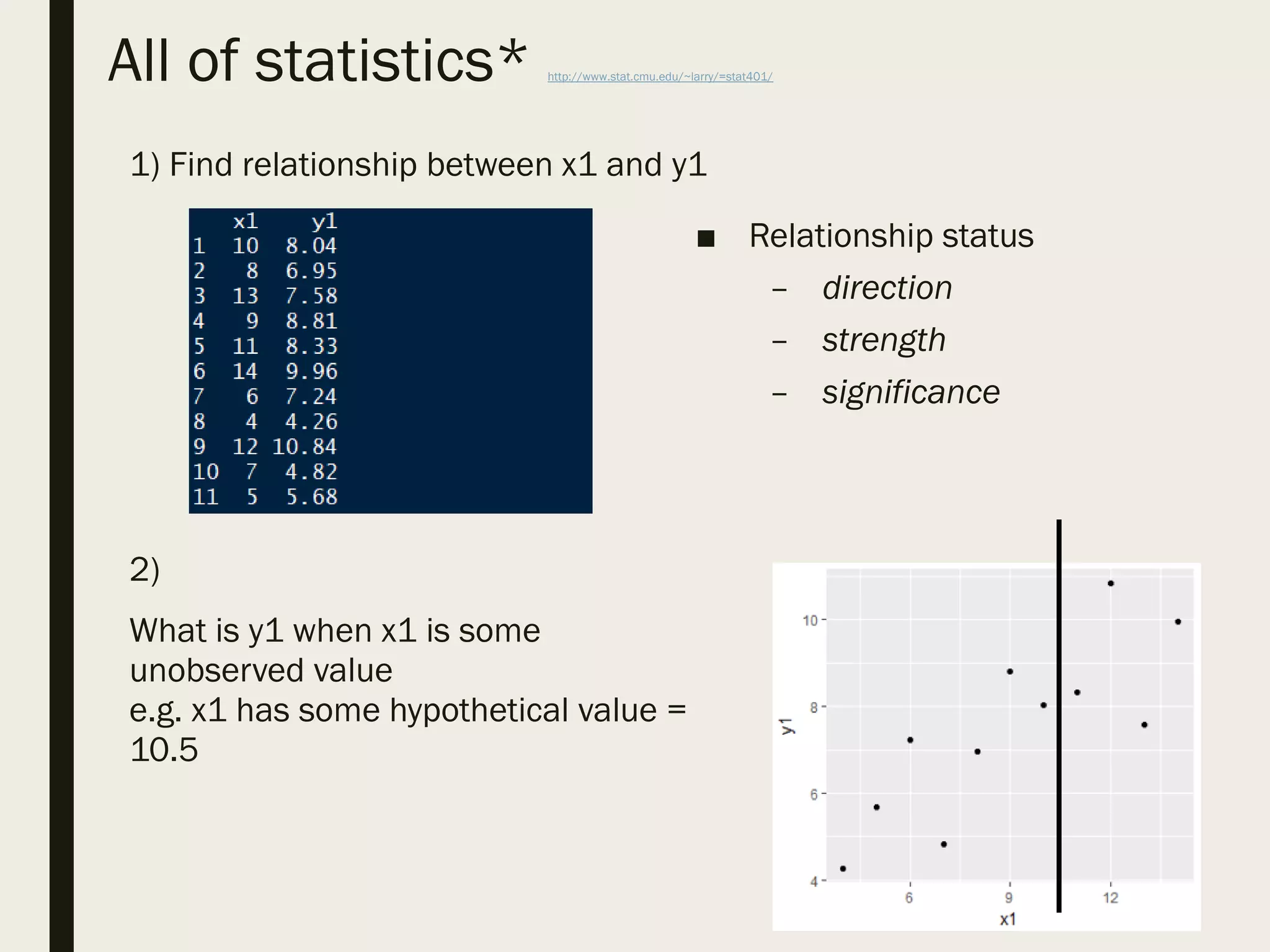
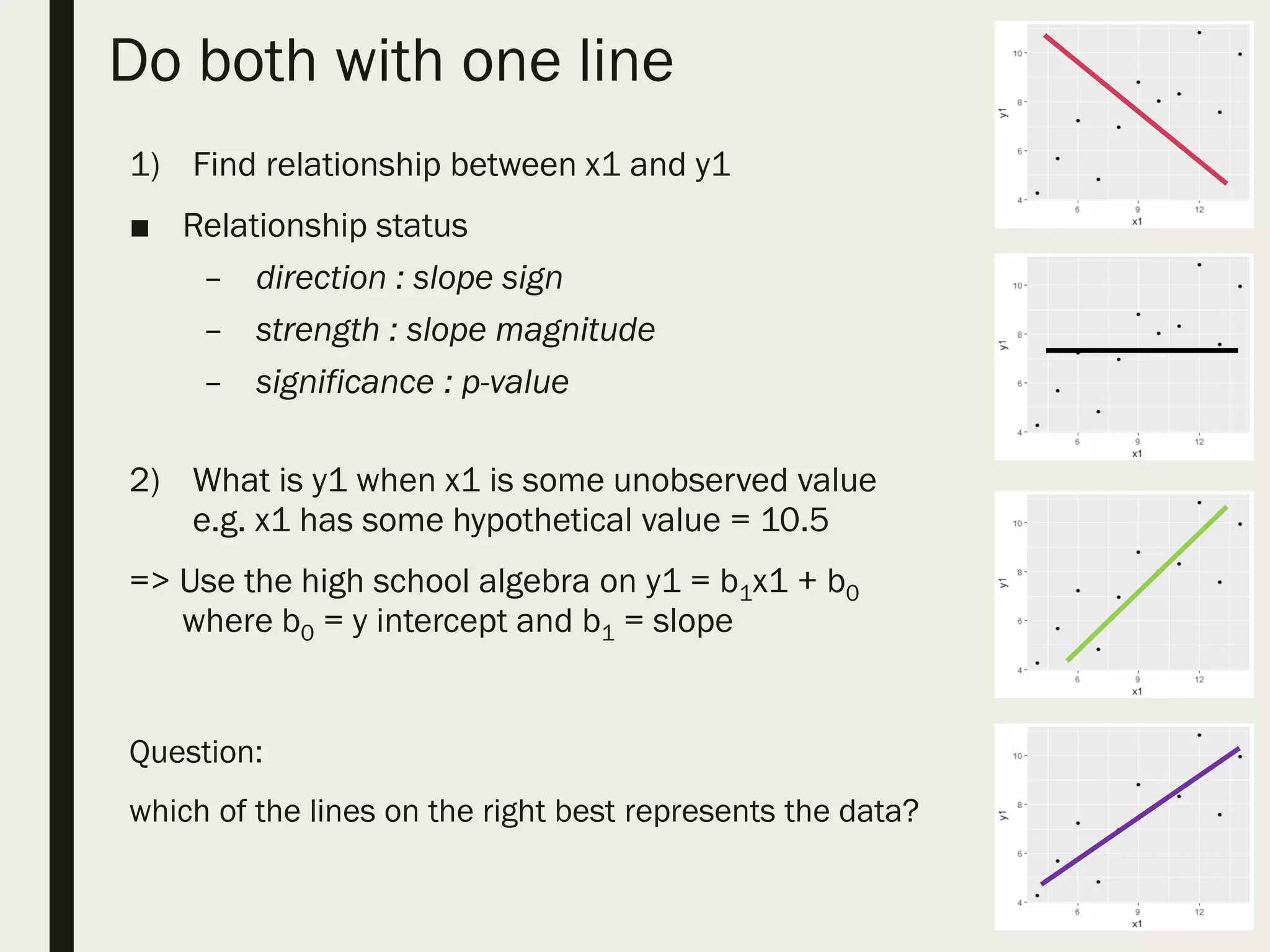
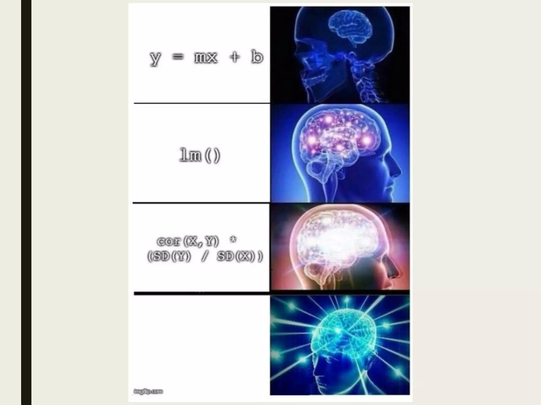
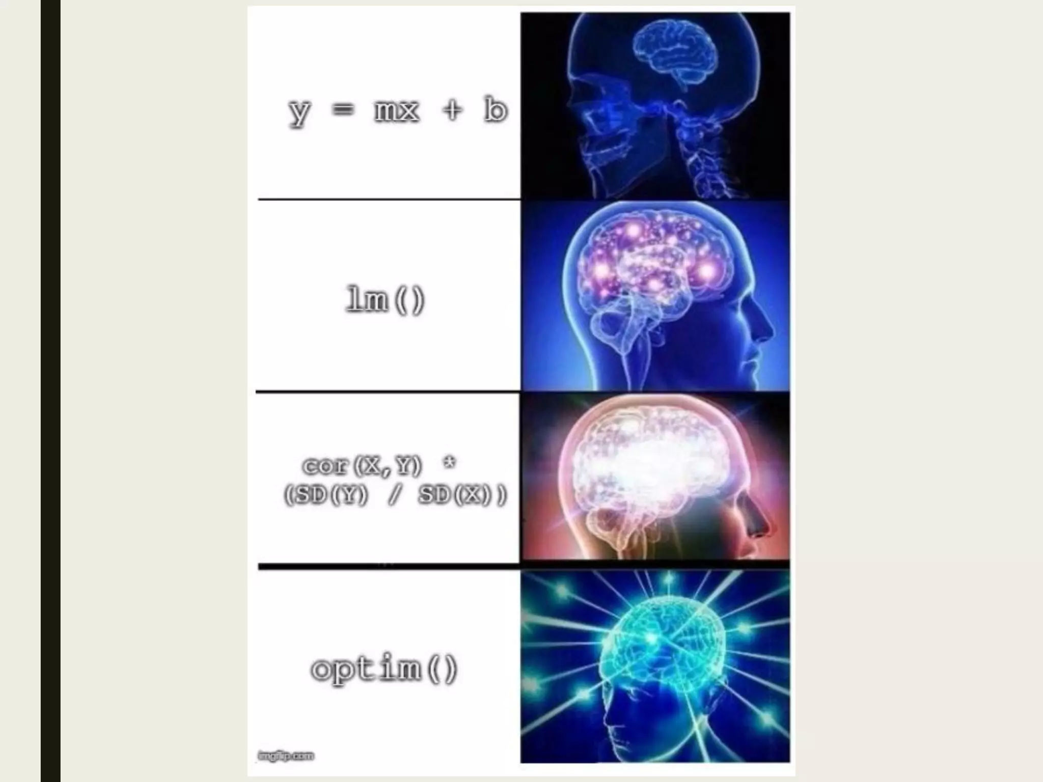
![What is the line of best fit?
■ Which line represents the data best?
■ This is where concepts like:
- Ordinary Least Squares,
- Maximum Likelihood Estimator,
- Sum of Squared Residuals
… and others are thrown around
■ Choose the line that has the smallest error
– ith real value : yi = b1xi + b0 + ei
– ith predicted value : ŷi = b1xi + b0
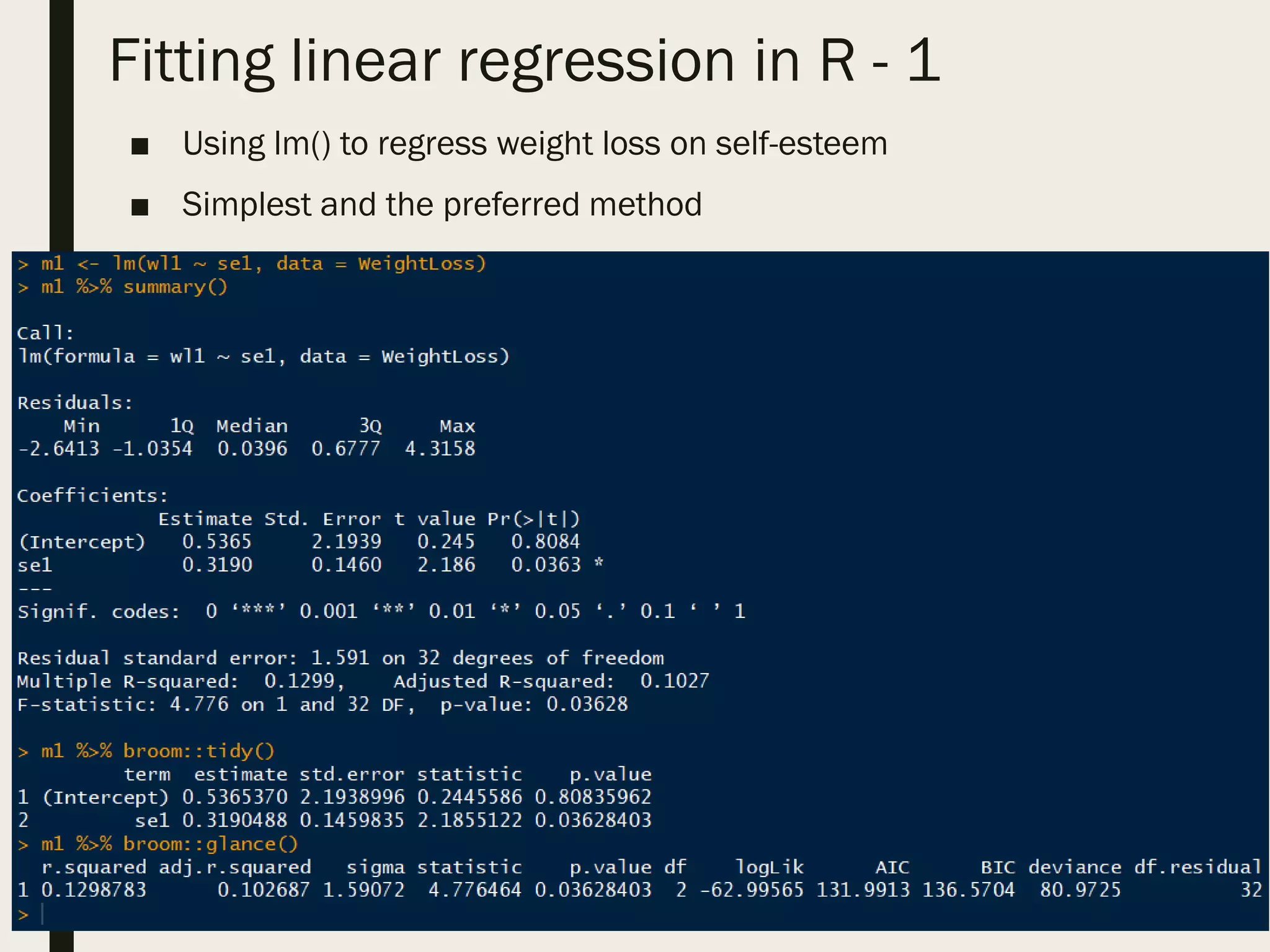
■ All of Statistics:
– All models minimize errors in prediction by
optimizing for a loss function.
– In linear regression, this is: Σ [(yi – ŷi)2]
■ b1 = how much y is expected to change if x increased by 1
b0 = what y is expected to be if x = 0](https://image.slidesharecdn.com/linearregression-180503215525/75/Linear-regression-in-R-9-2048.jpg)
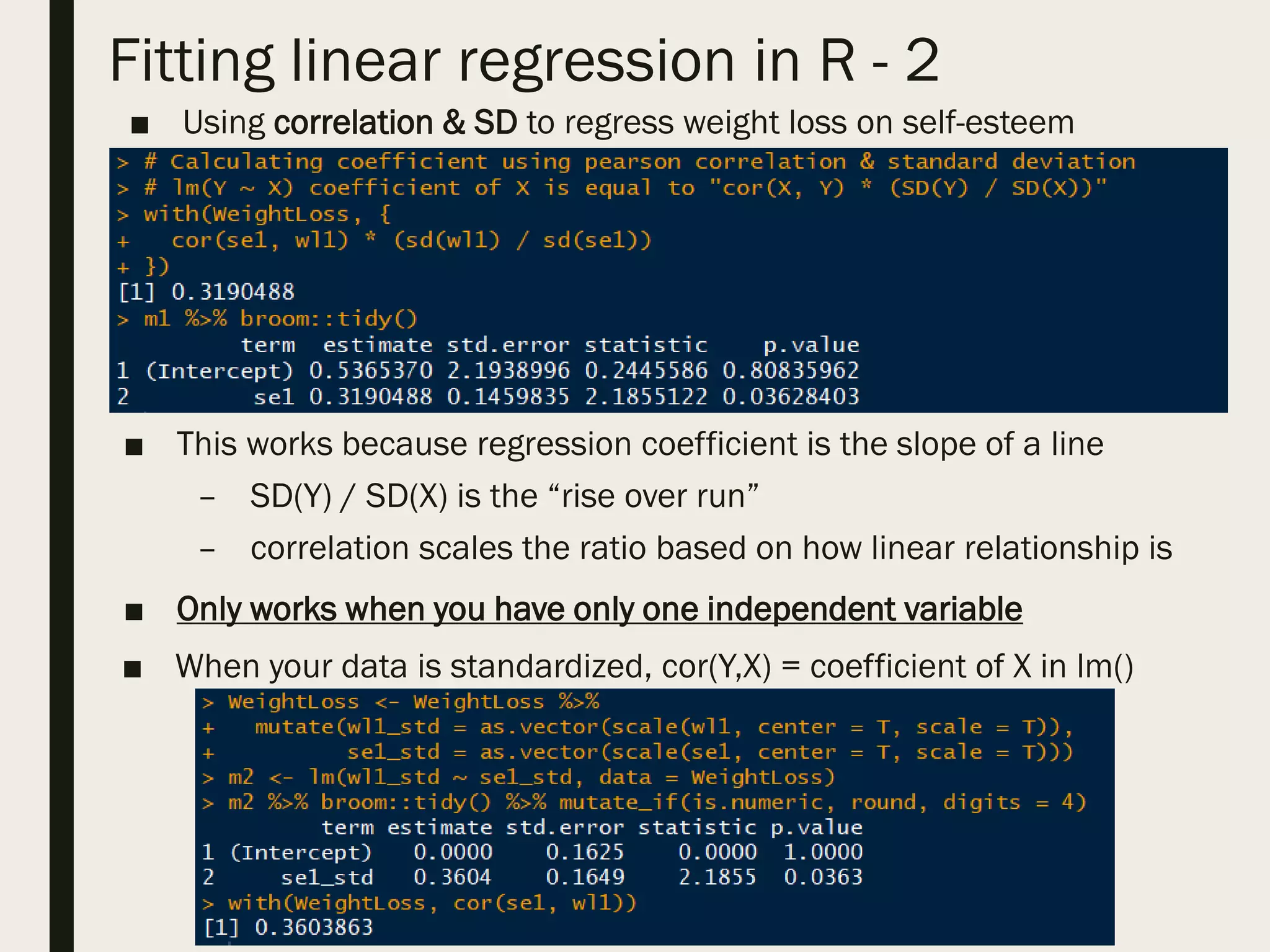
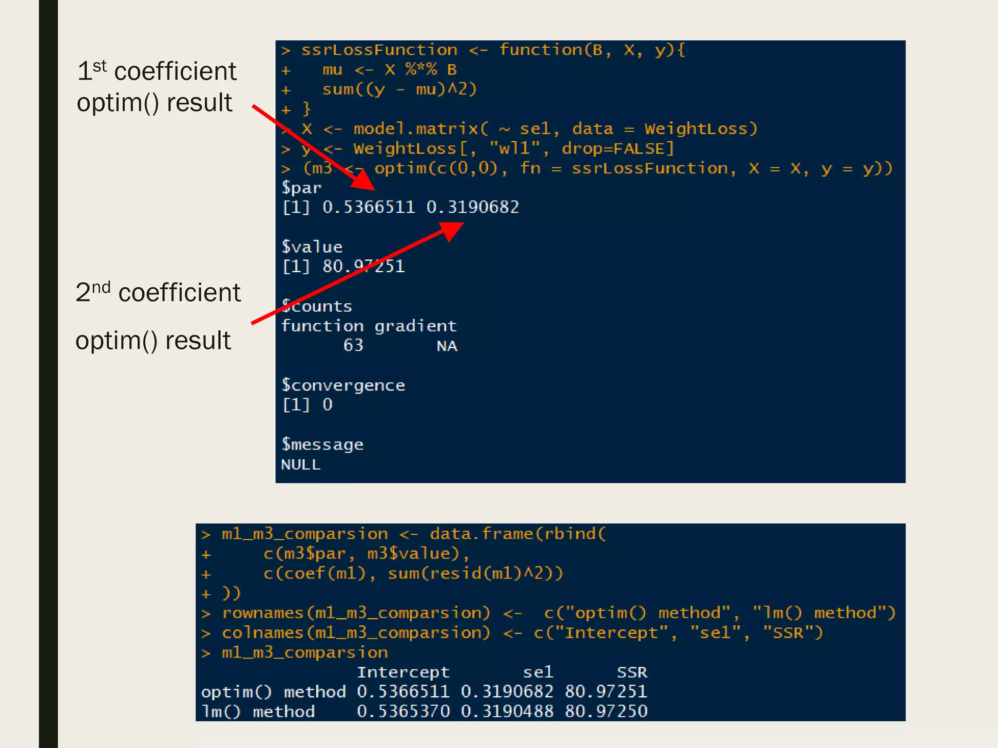
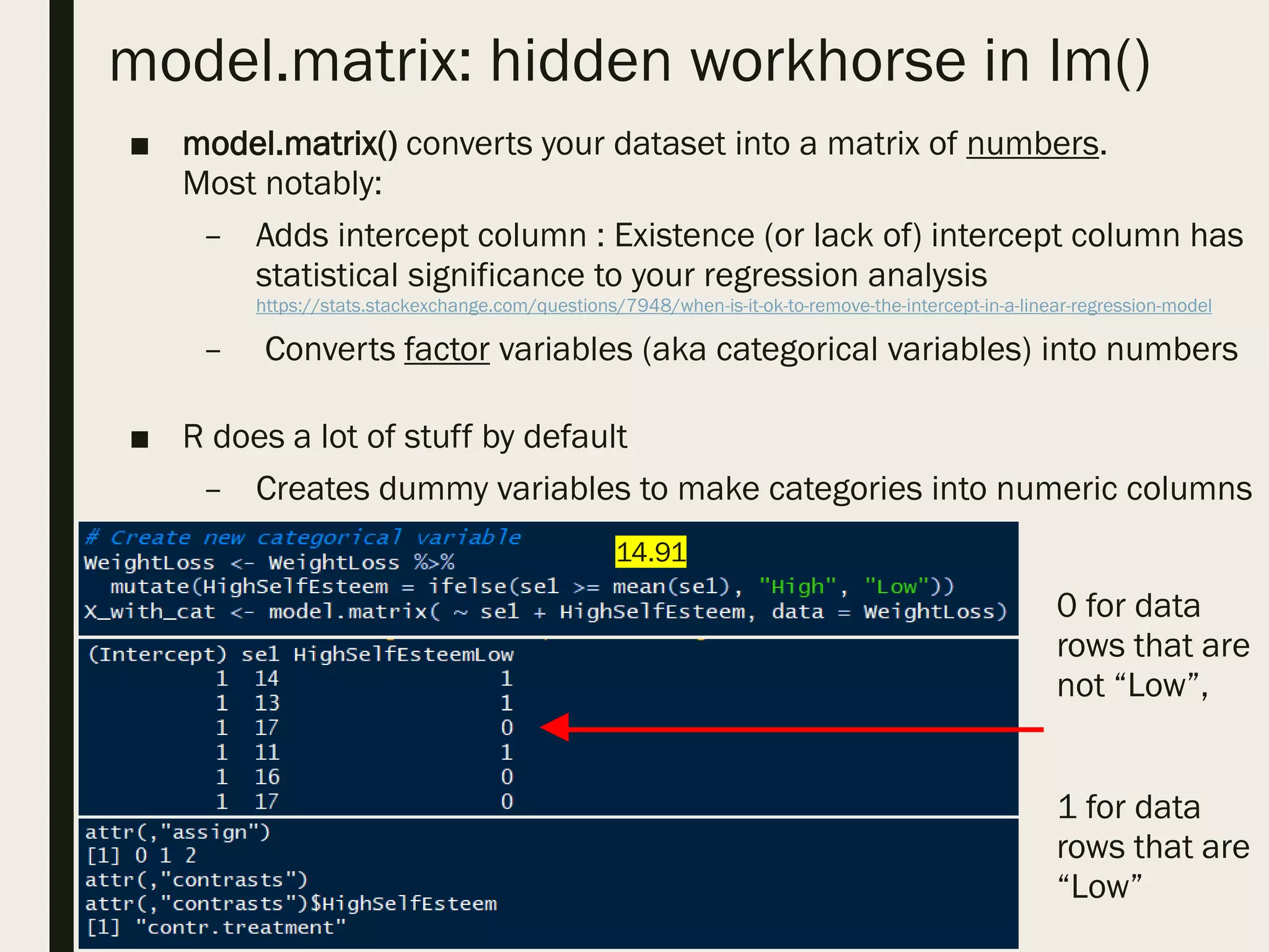
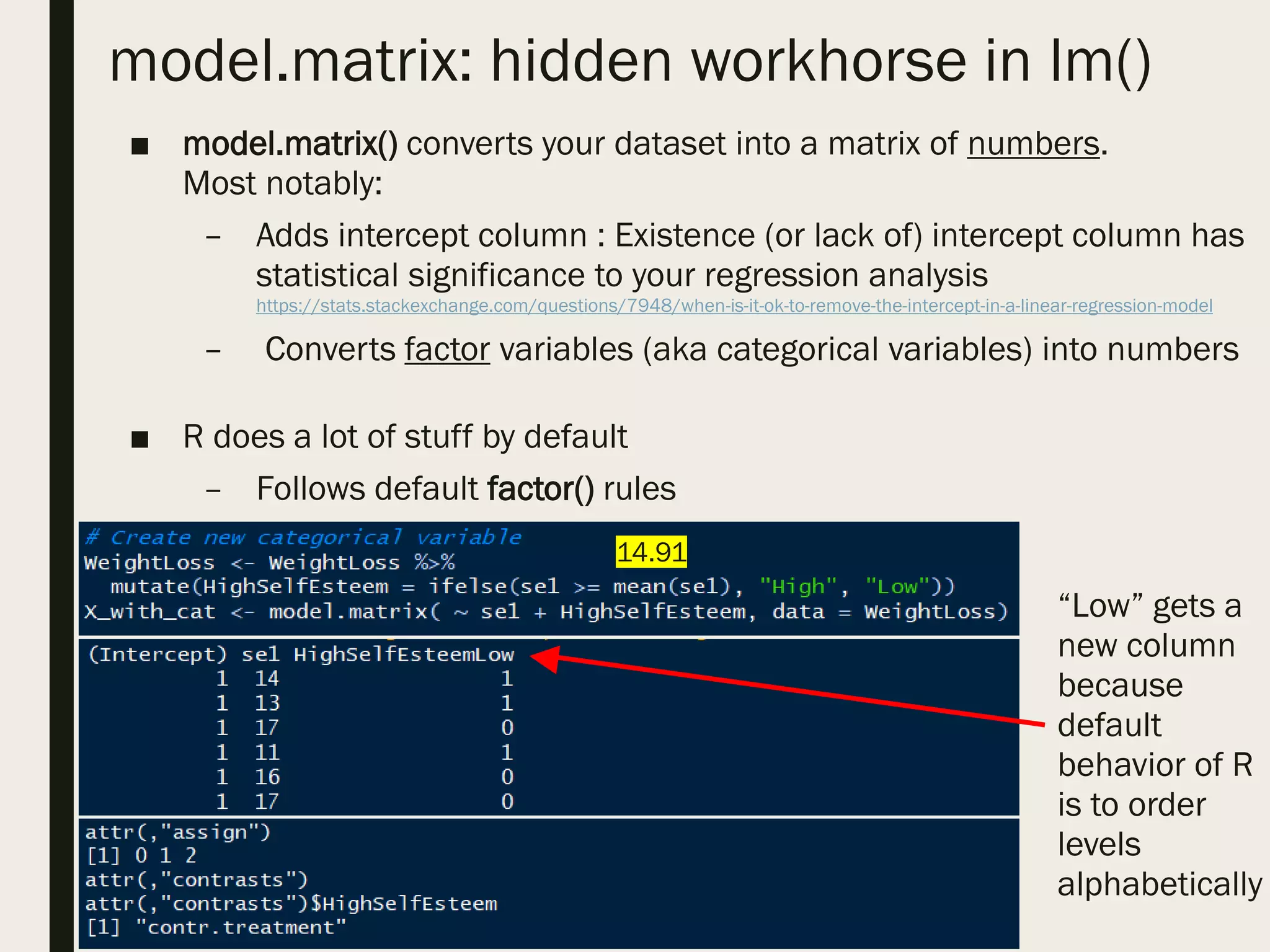
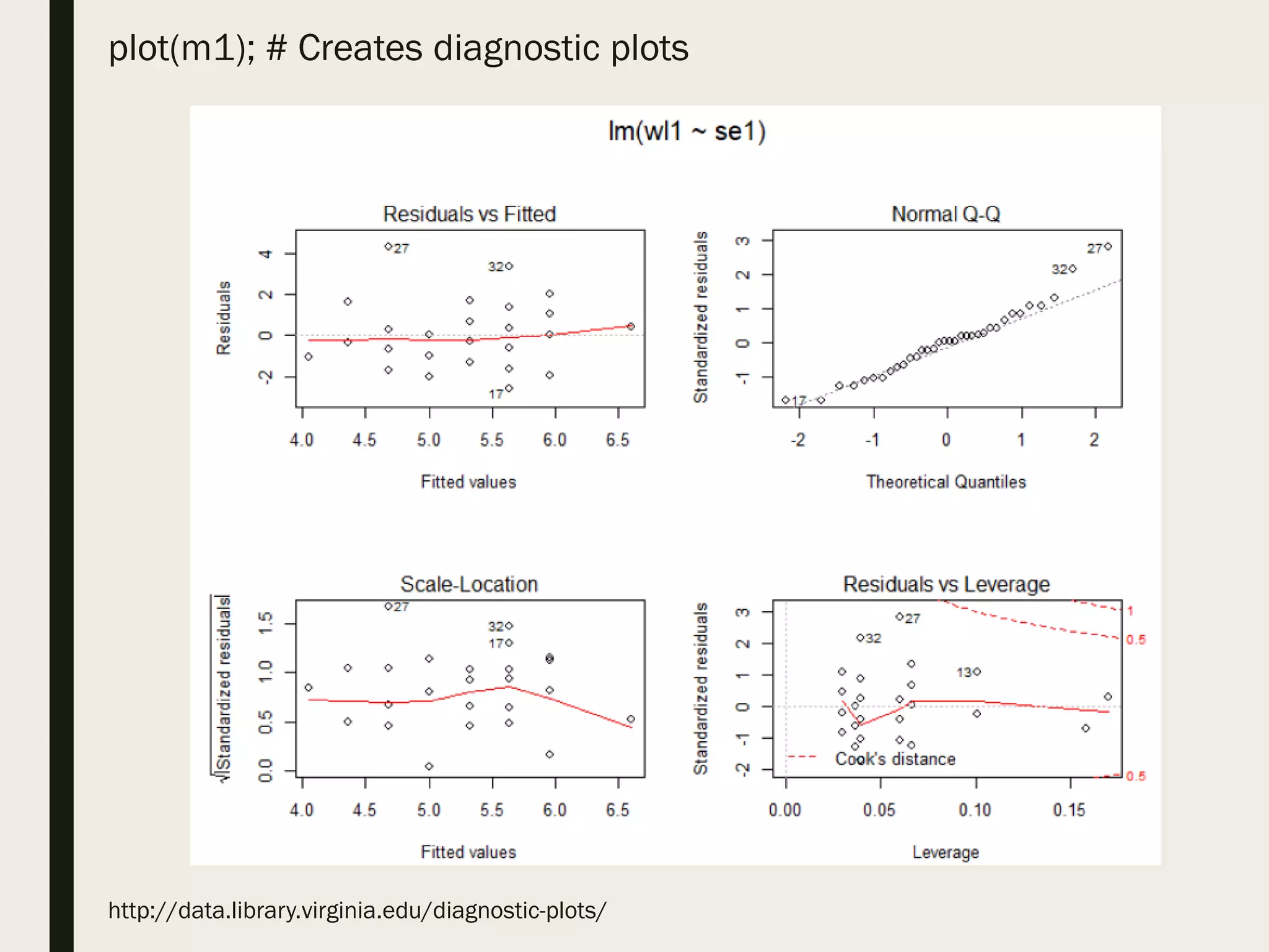
![Fitting linear regression in R - 3
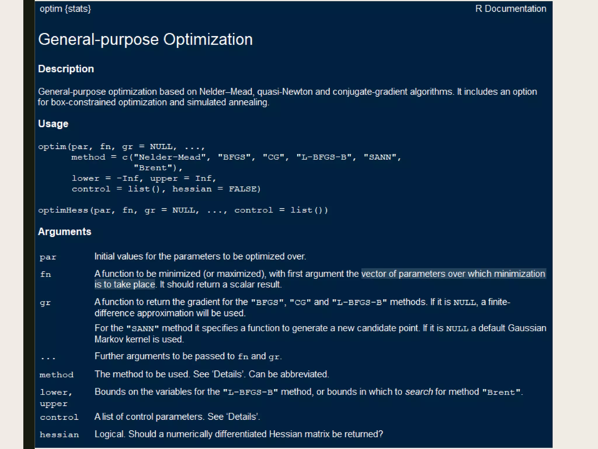
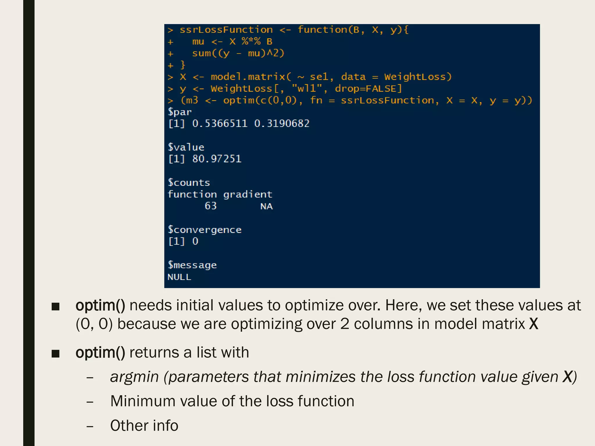
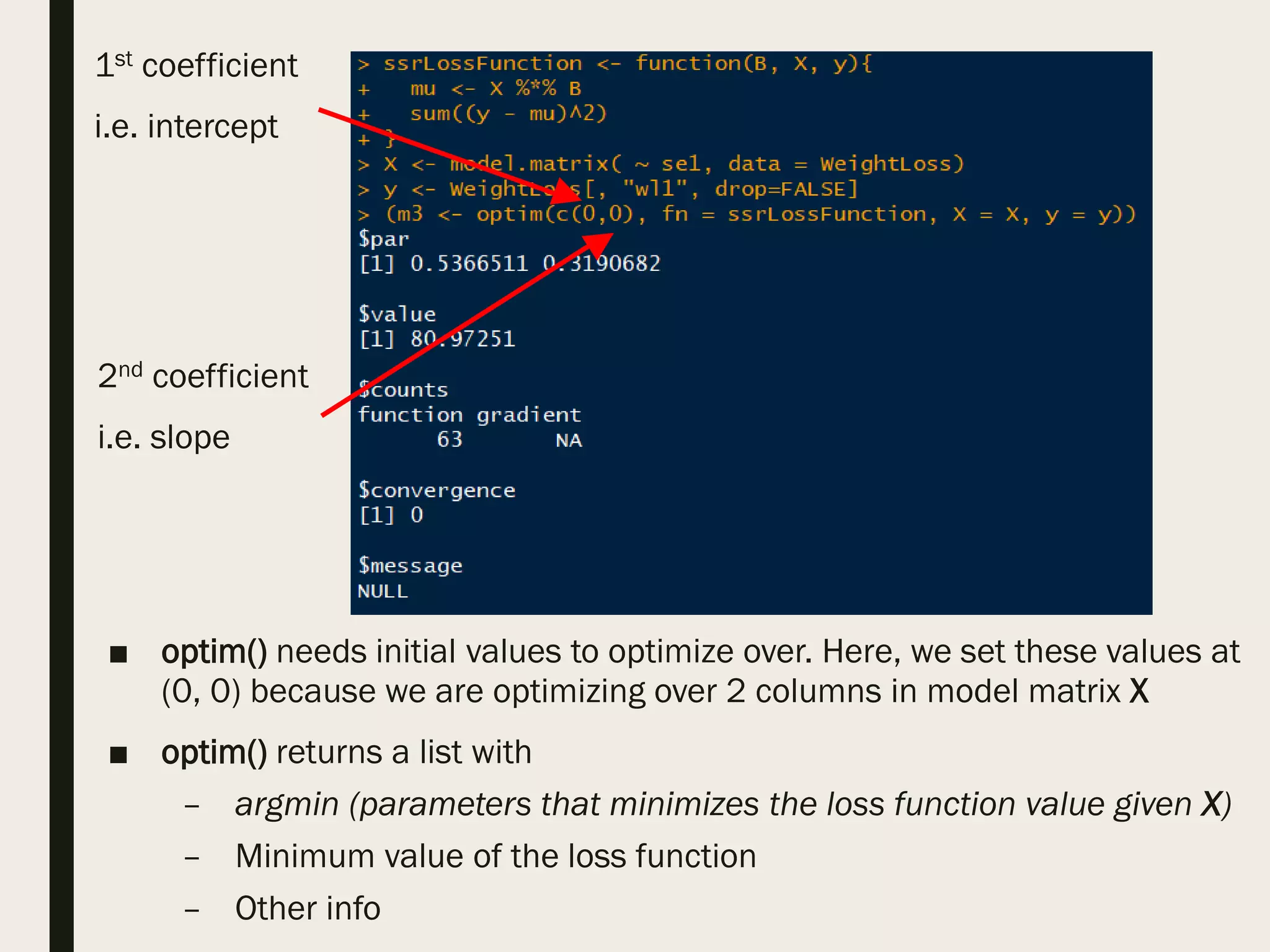
■ Using optim() and model matrix to regress weight loss on self-esteem
– optim() is a general-purpose optimizer
– Find coefficients that minimizes the loss function Σ [(yi – ŷi)2]
– Requires user to specify design matrix aka model matrix
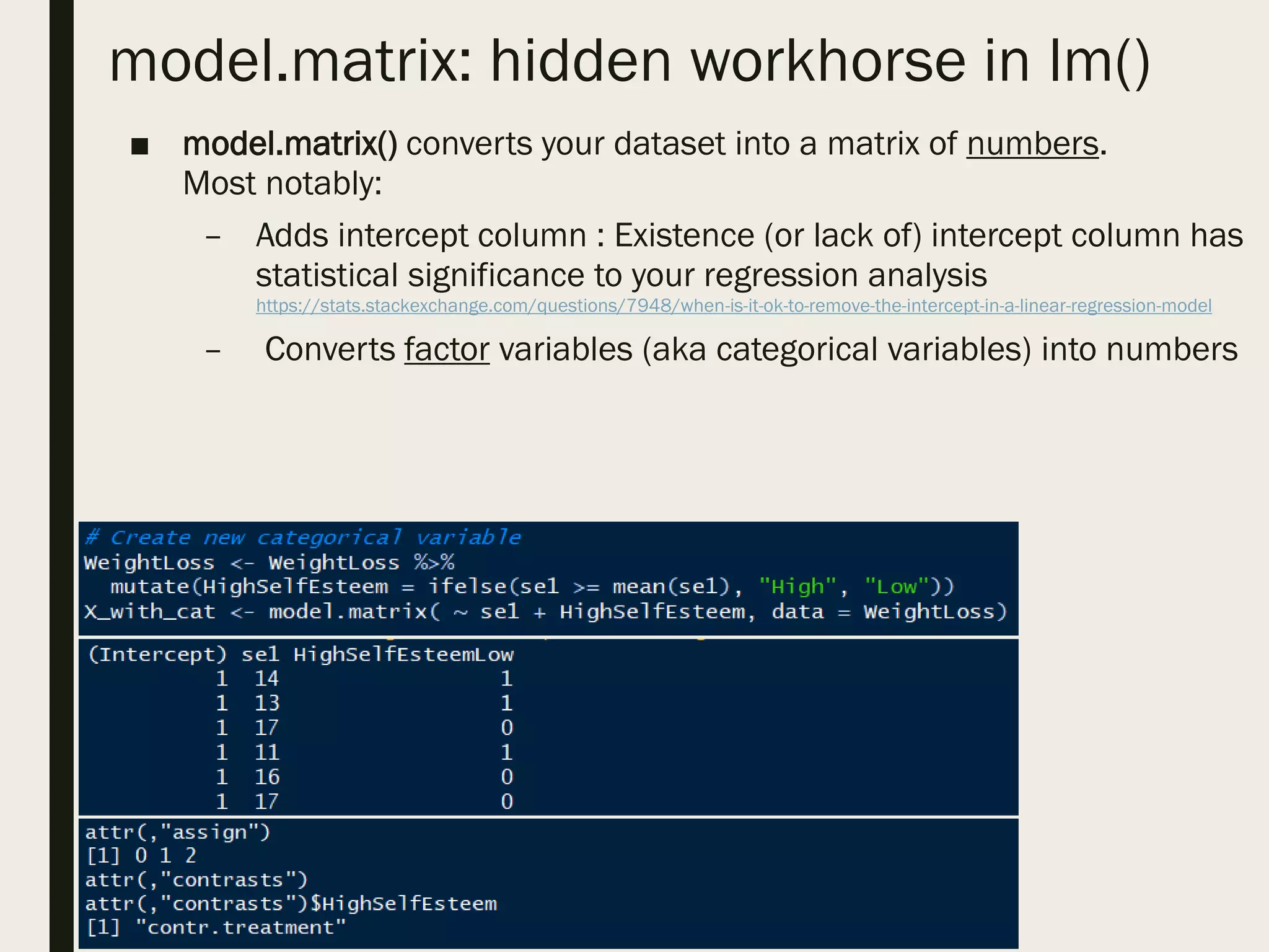
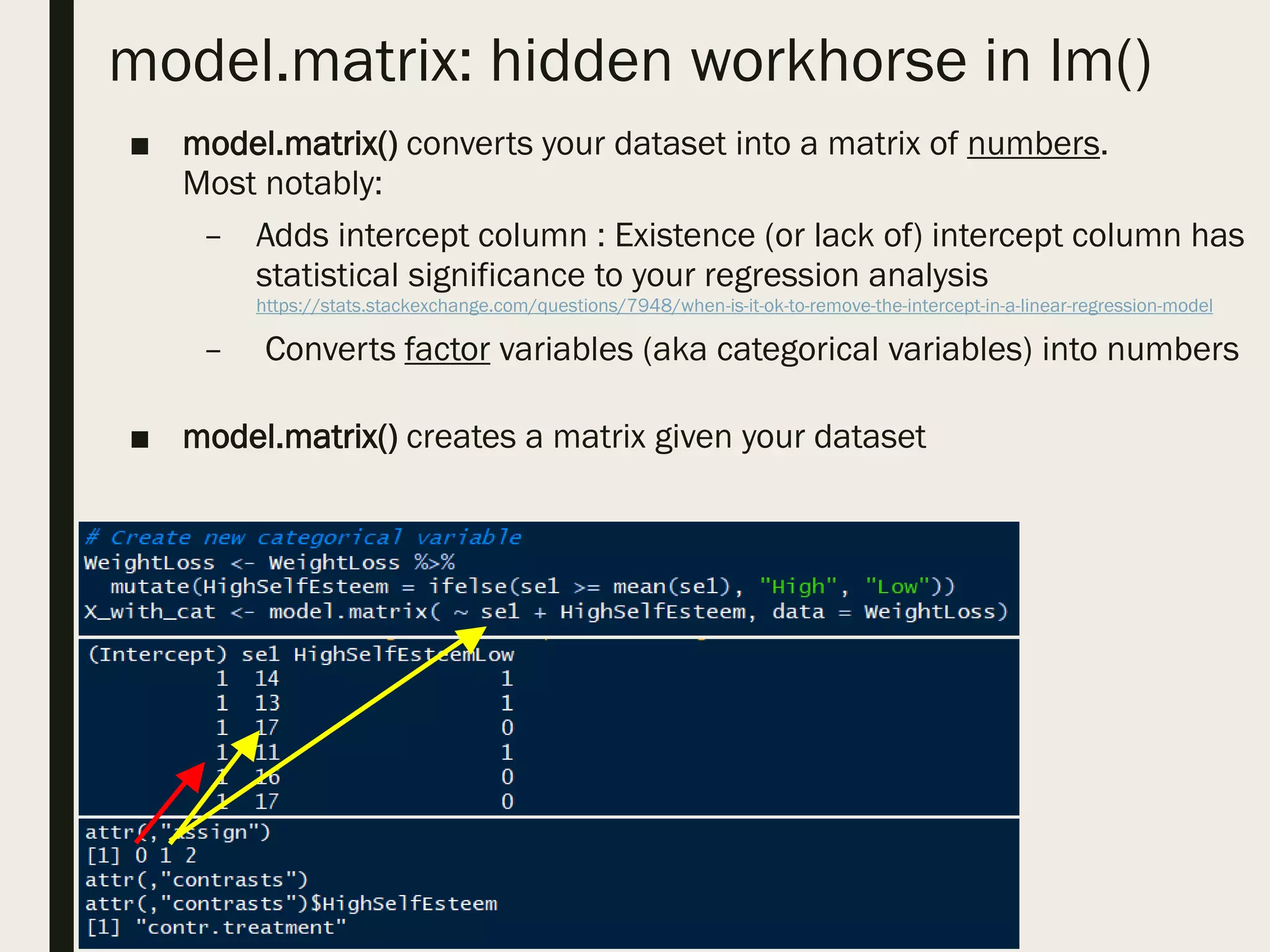
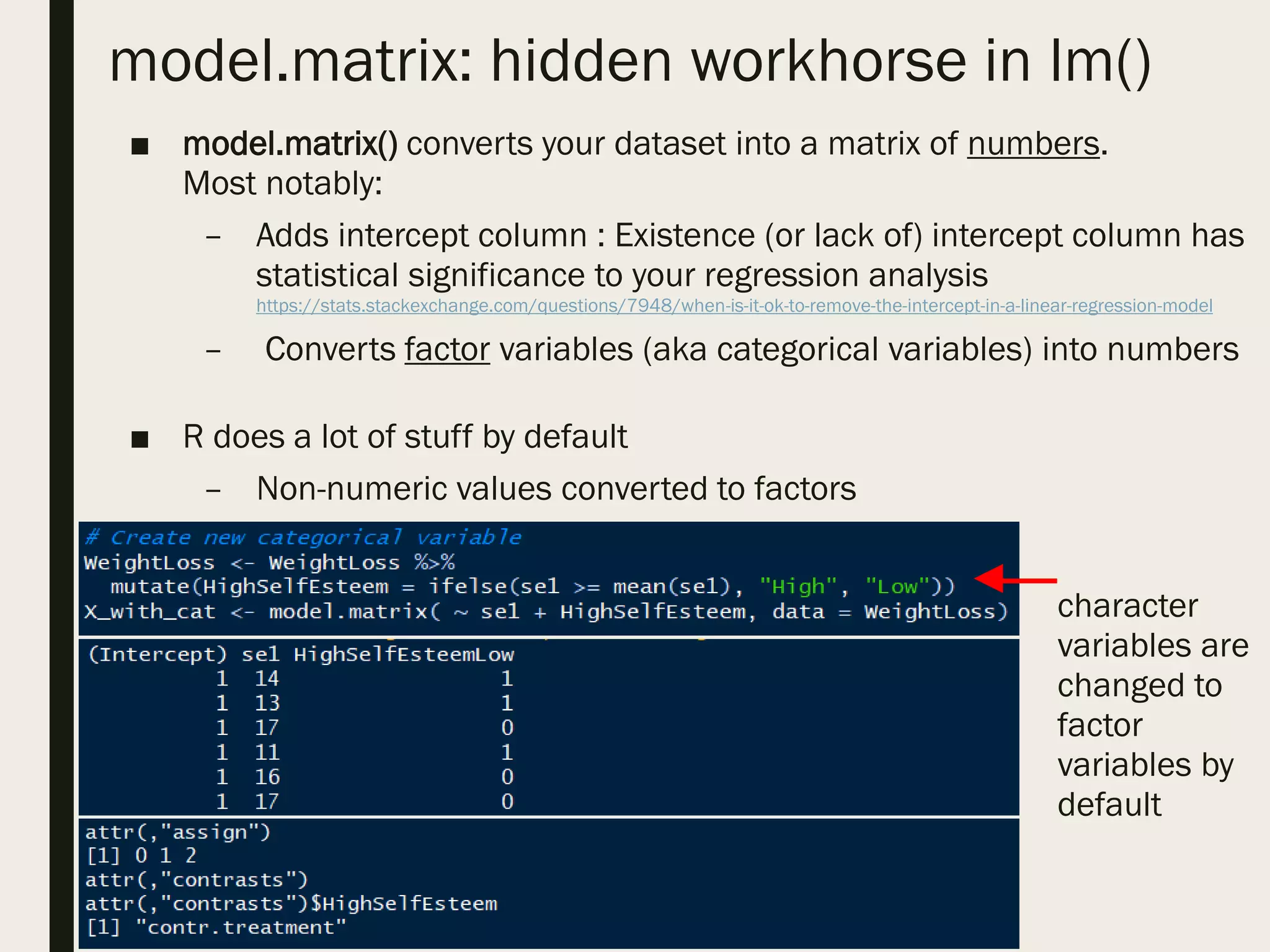
■ design matrix or model matrix
– This is abstracted away from you when you use formula in lm()
X y](https://image.slidesharecdn.com/linearregression-180503215525/75/Linear-regression-in-R-16-2048.jpg)


![[DSC Europe 25] Dusan Jovicic - AI Story: From on-prem to cloud and back agai...](https://cdn.slidesharecdn.com/ss_thumbnails/8kp49m6uq22ifnbwhfnk-2-251205085715-964d11a6-thumbnail.jpg?width=640&height=640&fit=bounds)


![[DSC Europe 25] Marija Vlajkovic & Andrea Radonjanin - Integration of AI tool...](https://cdn.slidesharecdn.com/ss_thumbnails/qf1jrglttoc3bm8s3aop-final-integration-of-ai-tools-251208151905-394f3a6a-thumbnail.jpg?width=640&height=640&fit=bounds)


![[DSC Europe 25] Nikola Rajovic - Hardware Technologies Under the Hood: RISC-V...](https://cdn.slidesharecdn.com/ss_thumbnails/o2gptrmtoyqndgoshwgq-dsc2025-tenstorrent-rajovic-251205090438-814685f5-thumbnail.jpg?width=640&height=640&fit=bounds)
![[DSC Europe 25] Dragan Vucic - Building the Learning Organization - How AI Tr...](https://cdn.slidesharecdn.com/ss_thumbnails/8brigo2sbu6qur6gxrra-7-251205085715-6ae07d24-thumbnail.jpg?width=640&height=640&fit=bounds)

![[DSC Europe 25] Dragana Ilic - AI for Big Data in Astronomy.pptx](https://cdn.slidesharecdn.com/ss_thumbnails/8palya86qaatvjhva1ms-2-dragana-ilic-ai-ilic-251208151906-652b819c-thumbnail.jpg?width=640&height=640&fit=bounds)


