This document discusses modeling and control of a 2 degree of freedom robot. It will: 1) Derive the forward and inverse kinematics of the robot using the proximal and distal D-H convention. 2) Calculate the Jacobian to relate joint velocities to end effector velocities. 3) Determine the dynamics of the robot using the Recursive Newton-Euler Formulation to calculate joint torques. 4) Generate a control scheme using these models to control the robot.

1. 
Abstract—Over the course of the semester in industrial
robotics, concepts taught in class will be applied to a real world
situation in the form of a 2 DOF RP (revolute, prismatic) robot. By
the conclusion of the semester, all work necessary in order to
generate a control schema for the aforementioned robot will be
completed. This procedure can then be replicated in other real
world situations (either in industry or academia) to control
various other classes of robot.
I. INTRODUCTION
2 DOF robotics platform (as pictured below) will be
undertaken.
Fig. 1. Two DOF robotics platform. Note that length “a” and angle “nu” are
constant and length “d” and angle “gamma” are variable (ie, the two
degrees of freedom
Included in this task will be modeling the forward
kinematics of platform using both the proximal D-H (Craig)
method and the distal D-H (Niku) method. Once the
forward modeling is complete, a MATLAB script replicating
the forward kinematics will be generated. This can be used
to determine the position of the end effector based upon
given joint variables.
Once this is complete, the inverse kinematics of the robot
will be found using the forward kinematics found
previously. The inverse kinematics of a robot can be used to
find the required joint variables to move to the end effector
to a given position. This will be crucial in order to generate
a scheme to “drive” the robot.
Next, the Jacobian matrix for the 2 DOF robot will be
found. The Jacobian matrix can be used to relate input
velocities (ie, joint velocities) into output velocities (ie, end
effector velocities) and vice versa.
However, the sections discussed above only address the
kinematics of the robot. The kinetics (dynamics) of the
robot still need to be determined in order to determine
required joint torques/forces to drive from one location to
another. The Recursive Newton Euler Formulation will be
used to derive the dynamics of the robot. While more
difficult to implement by hand than the Lagrange Energy
Method (another method used to determine joint
torques/forces), the Recursive Newton Euler Formulation is
useful since it is possible to implement through the use of a
MATLAB code or other computational tool.
In the sections to follow, each of the previously discussed
tasks will be laid out in greater detail, with requisite
drawings as well as computations. To start, observe the
proximal (Niku) D-H model.
II. PART 1 – PROXIMAL D-H MODELING
The proximal D-H method is one of many methods to
compute the position of the end effector of a robot. While
similar to the distal D-H method (Discussed in Section III),
the proximal D-H method differs in that it starts with the N-
th joint axes when placing link-frame origins. Due to this,
the method requires an individual to choose the zero frame
to match the one frame when joint variable one is zero and
choose the N-th frame arbitrarily (generally, to simplify the
math as much as possible). Using this method, the following
set of coordinate frames on the 2 DOF robot is as shown
below:
Fig. 2. Proximal D-H Coordinate Frames applied to the given 2 DOF
Robotics Platform
MEEN – 6931 Industrial Robotics – 2 DOF Robotics Project
Alex Folz, Marquette University MSME 2016

2. Note that for diagram in Fig. 2, X1 does not fall on the link
of length a. As such, it is pertinent to invoke trigonometry
to introduce the following relationships:
𝑎1 = a ∗ sin (
𝜋
2
− 𝜂) = 𝑎 ∗ cos⁡( 𝜂) (1)
𝑎2 = 𝑎 ∗ cos (
𝜋
2
− 𝜂) = 𝑎 ∗ sin⁡( 𝜂) (2)
Based upon the above relationships, a1 is the distance
between x1 and the intersection of link 1/link 2 along the z2
axis and a2 is the distance between the z1 axis and z2 axis
along the x1 axis. Now, one can use the following set of
rules to fill out the D-H table:
1. Assign θn as the angle from xn-1 to xn measured
about zn.
2. Assign dn as the distance from xn-1 to xn measured
along zn
3. Assign an-1 as the distance from zn-1 to zn measured
along xn-1
4. Assign αn-1 as the angle from zn-1 to zn measured
about xn-1.
Using these, the following D-H table was generated
based upon the chosen coordinate frames:
Table 1: Proximal D-H Parameters
N θn dn an-1 αn-1
1 γ+π/2-η 0 0 0
2 0 d+a1 a2 π/2
From the D-H table, it is now possible to derive the
homogenous rotation matrices from one frame to another
using the following matrix in addition to the following
trigonometric relationships for theta:
cos (𝛾 +
𝜋
2
− 𝜂) = sin⁡( 𝜂 − 𝛾) (3)
sin (𝛾 +
𝜋
2
− 𝜂) = cos⁡( 𝜂 − 𝛾) (4)
And finally, the rotation matrices for each frame as well
as the overall homogenous rotation matrix from the base
frame to the end effector are as follows:
𝑡1 =0
[
s(η − γ) −𝑐(𝜂 − 𝛾) 0 0
𝑐(𝜂 − 𝛾) 𝑠(𝜂 − 𝛾) 0 0
0 0 1 0
0 0 0 1
]
𝑡2 =1
[
1 0 0 𝑎2
0 0 1 𝑑 + 𝑎1
0 −1 0 0
0 0 0 1
]
𝑡2 =0
[
𝑠(𝜂 − 𝛾) 0 𝑐(𝜂 − 𝛾) 𝑎2 𝑠(𝜂 − 𝛾) + (𝑑 + 𝑎1)𝑐(𝜂 − 𝛾)
𝑐(𝜂 − 𝛾) 0 −𝑠(𝜂 − 𝛾) 𝑎2 𝑐(𝜂 − 𝛾) − (𝑑 + 𝑎1)𝑠(𝜂 − 𝛾)
0 1 0 0
0 0 0 1
]
Using the above matrix and a computational device
(MATLAB), the position of the end effector can now be
plotted relative to arbitrary inputs for joint variables. For
example, gamma and d were both incremented by 0.01 (in
radians and inches, respectively) with the following path
being plotted:
Fig. 3. Robot end effector path for specified values of gamma and d
III. PART 2 – DISTAL D-H MODELING
Similar to the proximal modeling done above, the
distal D-H method is also used to find the end effector
position of a robot based upon given joint variables.
However, it differs in that now, the N-th+1 joint axes
when placing link frame origins. Due to this, one will now
arbitrarily place the 0-th link frame origin (generally so
that the math simplifies the most) and pick the N-th link
frame origin to match the N-th -1 link frame origin when
joint variable N is 0. Returning to Section II, this is the
inverse of the proximal D-H method. Shown below are
the coordinate frames used to complete the distal D-H
modeling.
Fig. 4. Distal D-H Coordinate Frames applied to the given 2 DOF
Robotics Platform

3. Invoking the same trigonometric properties as in
section II, the following rules can be used to fill out a D-H
table:
1. Assign θn+1 as the angle from xn to xn+1 measured
about zn.
2. Assign dn+1 as the distance from xn to xn+1
measured along zn
3. Assign an+1 as the distance from zn to zn+1 measured
along xn+1
4. Assign αn+1 as the angle from zn to zn+1 measured
about xn+1.
Using these, the following D-H table was generated
based upon the chosen coordinate frames:
Table 2: Distal D-H Parameters
N θn dn an-1 αn-1
0 γ+π/2-η 0 a2 π/2
1 0 d+a1 0 0
Since the rules for defining each value in the D-H table
has changed from the proximal method, so too does the
homogenous transformation matrix that can be used to go
from one frame to another. This “new” matrix is as below:
And finally, the rotation matrices for each frame as well
as the overall homogenous rotation matrix from the base
frame to the end effector are as follows:
𝑡1 =0
[
s(η − γ) 0 𝑐(𝜂 − 𝛾) 𝑎2 𝑠(𝜂 − 𝛾)
𝑐(𝜂 − 𝛾) 0 −𝑠(𝜂 − 𝛾) 𝑎2 𝑐(𝜂 − 𝛾)
0 1 0 0
0 0 0 1
]
𝑡2 =1
[
1 0 0 0
0 1 1 0
0 0 1 𝑑 + 𝑎1
0 0 0 1
]
𝑡2 =0
[
𝑠(𝜂 − 𝛾) 0 𝑐(𝜂 − 𝛾) 𝑎2 𝑠(𝜂 − 𝛾) + (𝑑 + 𝑎1)𝑐(𝜂 − 𝛾)
𝑐(𝜂 − 𝛾) 0 −𝑠(𝜂 − 𝛾) 𝑎2 𝑐(𝜂 − 𝛾) − (𝑑 + 𝑎1)𝑠(𝜂 − 𝛾)
0 1 0 0
0 0 0 1
]
Since the final homogeneous rotation matrix from the
base frame to the end effector matches the matrix from
Section II (proximal DH), a plot showing the path of the
end effector of the robot using the above matrix would
match the plot shown in Fig. 3.
IV. PART 3 – INVERSE KINEMATICS
Having confirmed the validity of the forward
kinematics through the comparison of distal results with
proximal results, it is now possible to find the inverse
kinematics of the robot. This can be done setting the final
homogeneous rotation matrix equal to the NOA matrix as
shown below:
[
𝑛 𝑥 𝑜 𝑥 𝑎 𝑥 𝑃𝑥
𝑛 𝑦 𝑜 𝑦 𝑎 𝑦 𝑃𝑦
𝑛 𝑧 𝑜_𝑧 𝑎_𝑧 𝑃𝑧
0 0 0 1
]
=⁡[
𝑠(𝜂 − 𝛾) 0 𝑐(𝜂 − 𝛾) 𝑎2 𝑠(𝜂 − 𝛾) + (𝑑 + 𝑎1)𝑐(𝜂 − 𝛾)
𝑐(𝜂 − 𝛾) 0 −𝑠(𝜂 − 𝛾) 𝑎2 𝑐(𝜂 − 𝛾) − (𝑑 + 𝑎1)𝑠(𝜂 − 𝛾)
0 1 0 0
0 0 0 1
]
Now, observe the fourth column of the matrix to
generate the following set of equations:
𝑃𝑥 = 𝑎2 𝑠(𝜂 − 𝛾) + (𝑑 + 𝑎1)𝑐(𝜂 − 𝛾) (5)
𝑃𝑦 = 𝑎2 𝑐(𝜂 − 𝛾) − (𝑑 + 𝑎1)𝑠(𝜂 − 𝛾) (6)
𝑃𝑧 = 0 (7)
Finally, use algebra to generate two equations that
solve for d and γ independently in terms of Px and Py.
Begin by solving for d in Eqs. (5 & 6) as shown below,
noting that 𝛽 = 𝜂 − 𝛾:
𝑑 =
(𝑥−𝑎2∗sin(𝛽)−𝑎1∗cos(𝛽))
𝑐𝑜𝑠(𝛽)
(5a)
𝑑 =
(−𝑦+𝑎2∗cos(𝛽)−𝑎1∗sin(𝛽))
𝑠𝑖𝑛(𝛽)
(6a)
Now, if Eqs. (5a & 6a) are set equal to one another, it is
possible to solve for beta in terms of x & y independently
of d.
(−𝑦+𝑎2∗cos(𝛽)−𝑎1∗sin(𝛽))
𝑠𝑖𝑛(𝛽)
=
(−𝑦+𝑎2∗cos(𝛽)−𝑎1∗sin(𝛽))
𝑠𝑖𝑛(𝛽)
(8)
Or:
𝑥 ∗ sin(𝛽) + 𝑦 ∗ cos(𝛽) = 𝑎2 (8a)
Finally, to solve for beta, trig properties can be invoked
or it can be solved using a symbolic mathematics
solver such as maple or Wolfram Alpha. Using Wolfram
Alpha yields:

4. 𝛽 = 2 ∗ tan−1
(
𝑥−𝑠𝑞𝑟𝑡(−𝑎2
2+𝑥2+𝑦2)
𝑎2+𝑦
) (9)
Having solved for beta, it can now be subbed back into
either Eq. (5a) or Eq. (6a) to solve for d. This completes
the inverse kinematic solution for the robot.
V. PART 4 – JACOBIAN & INVERSE JACOBIAN
Now that the position of the end effector of the robot
is fully defined through the use of forward and inverse
kinematics, it is now time to define the time derivative of
position, velocity, of the end effector of the robot in
terms of the velocities of the joints and vice versa. The
Jacobian and inverse Jacobian can be employed to handle
this task. In general, the Jacobian is defined by the
following function:
Applying this function to the 2 DOF robot presented
yields the following matrix based relationship between
end effector velocities and joint velocities:
[
𝑥̇
𝑦̇
] = [
𝐽11
𝑇0
𝐽12
𝑇0
𝐽21
𝑇0
𝐽22
𝑇0
] [
𝛾̇
𝑑̇
] (10)
However, the Jacobian must first be found in the end
effector frame. Since this will be multiplied through by
the rotation matrix, all 6 values in each of the columns of
the Jacobian must be found. This can be done with the
following set of equations:
𝐽11
𝑇2
= (−𝑛 𝑥 𝑝 𝑦 + 𝑛 𝑦 𝑝 𝑥) (11)
𝐽12
𝑇2
= (−𝑜 𝑥 𝑝 𝑦 + 𝑜 𝑦 𝑝 𝑥) (12)
𝐽13
𝑇2
= (−𝑎 𝑥 𝑝 𝑦 + 𝑎 𝑦 𝑝 𝑥) (13)
𝐽14
𝑇2
= (𝑛 𝑧) (14)
𝐽15
𝑇2
= (𝑜𝑧) (15)
𝐽16
𝑇2
= (𝑎 𝑧) (16)
𝐽21
𝑇2
= (𝑛 𝑧) (17)
𝐽22
𝑇2
= (𝑜𝑧) (18)
𝐽23
𝑇2
= (𝑎 𝑧) (19)
𝐽24
𝑇2
= (0) (20)
𝐽25
𝑇2
= (0) (21)
𝐽26
𝑇2
= (0) (22)
Using values from the NOA matrix as shown below, it is
now possible to solve for each value in the J matrix:
[
𝑛 𝑥 𝑜 𝑥 𝑎 𝑥 𝑃𝑥
𝑛 𝑦 𝑜 𝑦 𝑎 𝑦 𝑃𝑦
𝑛 𝑧 𝑜𝑧 𝑎 𝑧 𝑃𝑧
0 0 0 1
] =
⁡[
𝑠(𝜂 − 𝛾) 0 𝑐(𝜂 − 𝛾) 𝑎2 𝑠(𝜂 − 𝛾) + (𝑑 + 𝑎1)𝑐(𝜂 − 𝛾)
𝑐(𝜂 − 𝛾) 0 −𝑠(𝜂 − 𝛾) 𝑎2 𝑐(𝜂 − 𝛾) − (𝑑 + 𝑎1)𝑠(𝜂 − 𝛾)
0 1 0 0
0 0 0 1
]
Plugging in all 12 values required yields the following
matrix:
𝐽 =
𝑇2
[
𝑑 + 𝑎1 0
0 0
−𝑎2 1
0 0
1 0
0 0]
To find the Jacobian in the base frame (useful for finding
joint velocities and singularities), it will be required to
multiply the Jacobian in the end effector frame by the
rotation transformation matrix from the end effector frame
to the base frame in the following form in Eq. (23):
𝐽 =
𝑇0
[
𝑅2
0
0 0 0
0 0 0
0 0 0
0 0 0
0 0 0
0 0 0
𝑅2
0
]
𝐽
𝑇2
(23)
Completing this multiplication yields the Jacobian in the
base frame. The Jacobian relates known velocities in joint
space (in this case, the derivatives of gamma and d) to
velocities in cartesian (or cylindrical, spherical, etc.) space.
This was shown in Eq. (10). Subbing in values of the first two
rows found in Eq. (23) (as this robot only has 2 DOF) yields
the following:
[
𝑥̇
𝑦̇
] = [
(𝑎1 + 𝑑) sin(𝜂 − 𝛾) − 𝑎2cos⁡( 𝜂 − 𝛾) cos⁡( 𝜂 − 𝛾)
(𝑎1 + 𝑑) cos(𝜂 − 𝛾) + 𝑎2sin⁡( 𝜂 − 𝛾) sin(𝜂 − 𝛾)
] [
𝛾̇
𝑑̇
]
(10a)
In addition, it will be useful to find the inverse Jacobian
matrix, which relates input joint velocities to end effector
velocities and is as follows:
[
𝛾̇
𝑑̇
]
=
1
−(𝑎1 + 𝑑)
[
sin⁡( 𝜂 − 𝛾) −cos⁡( 𝜂 − 𝛾)
−(𝑎1 + 𝑑) cos(𝜂 − 𝛾) − 𝑎2sin⁡( 𝜂 − 𝛾) (𝑎1 + 𝑑) sin(𝜂 − 𝛾) − 𝑎2cos⁡( 𝜂 − 𝛾)
] [
𝑥̇
𝑦̇
]
(10b)

5. Finally, singularities can be found using the determinate
of the Jacobian in the 0 frame. This will be useful to
determine locations at which infinite joint velocities will be
needed to achieve certain end effector velocities. In a
practical application, these positions should be avoided if at
all possible.
det⁡( 𝐽) = 0
𝑇0
(24)
𝑑 = −𝑎1
VI. PART 5 –DYNAMIC ANALYSIS USING RECURSIVE
NEWTON-EULER FORMULATION
With the velocity analysis of the 2 DOF robot now
complete, it is possible to move on to the acceleration
and force (dynamic) analysis of the robot. To do so, the
recursive Newton-Euler (RNE) formulation will be
employed. The RNE approach to dynamic modeling is a
computer programmable way of finding the dynamics of
a system by using an algorithmic-based set of coordinate
frames. Often times, it is used on multi DOF systems as
the dynamic analysis of systems rapidly becomes more
complex as the number of DOF increases. Begin this
method by recalling the rotation matrices (as well as the
coordinate systems as seen in Fig. 4) generated from the
Distal Variant D-H procedure completed earlier:
𝐴1 = [
s(η − γ) 0 𝑐(𝜂 − 𝛾) 𝑎2 𝑠(𝜂 − 𝛾)
𝑐(𝜂 − 𝛾) 0 −𝑠(𝜂 − 𝛾) 𝑎2 𝑐(𝜂 − 𝛾)
0 1 0 0
0 0 0 1
]
𝐴2 = [
1 0 0 0
0 1 1 0
0 0 1 𝑑 + 𝑎1
0 0 0 1
]
The transposed 3x3 rotation matrix from each will be
used extensively through the remainder of the analysis.
Working up towards finding the torque or force applied by
each joint, begin by finding the angular velocity at each
joint (note that for each step, equations will differ when
observing a prismatic joint vs. a revolute joint):
𝜔⃑⃑ 1 = 𝑅0( 𝜔⃑⃑0
0 + [
0
0
1
] 𝛾)̇11
(25)
𝜔⃑⃑ 1 =⁡[
0
𝛾̇
0
]1
𝜔⃑⃑ 2 = 𝑅1( 𝜔⃑⃑1
1)22
(26)
𝜔⃑⃑ 2 =⁡[
0
𝛾̇
0
]2
Similarly, to find the angular acceleration of each joint:
𝛼1 = 𝑅0( 𝛼0
0 + ⌈
0
0
1
⌉11
𝛾̈ + 𝜔⃑⃑0
0 𝑋 [
0
0
1
] 𝛾̇) (27)
𝛼1 =⁡[
0
𝛾̈
0
]1
𝛼1 = 𝛼2
2
=⁡[
0
𝛾̈
0
]1
Next, to find the radius to each coordinate system and
the linear velocity of each:
𝑟𝑖
𝑖
= [
𝑎𝑖
𝑑𝑖sin⁡( 𝛼𝑖)
𝑑𝑖cos⁡(αi)
] (28)
𝑟1
1
= [
𝑎2
0
0
]
𝑟2
2
= [
0
0
𝑑 + 𝑎1
]
𝑣1 = 𝑅1
01
𝑣0
0 + 𝜔⃑⃑ 1⁡𝑥 𝑟1
11
(29)
𝑣1 = [
0
0
−𝑎2 𝛾̇
]1
𝑣2 = 𝑅2
12
( 𝑣1
1 + [
0
0
1
] 𝑑̇2) + 𝜔⃑⃑ 2⁡𝑥 𝑟2
22
(30)
𝑣2 = [
𝛾̇( 𝑑 + 𝑎1)
0
𝑑̇ − 𝑎2 𝛾̇
]2
At this point, the equations in use became exceedingly
complex. As such, MATLAB was used to assist in the
calculation of each successive step in the RNE method.
However, the calculations for each of these steps can be
seen in the RNE formulation code found in Appendix A of
this report. Looking at the final step, the Equations of
motion (depicted in matrix form) are as below:
𝑚(𝜃̈)
= [ 𝑚1 (
1
4
𝑎2
) + 𝑚2(𝐿2
2
− 2𝐿2(𝑎 + 𝑑) + 𝑎2
+ 2𝑎1 𝑑 + 𝑑2) + 𝐼1 + 𝐼2 −𝑚2 𝑎2
−𝑚2 𝑎2 𝑚2
]
(31)

6. 𝑣(𝜃, 𝜃̇) = [
2𝑚2(𝑎1 + 𝑑 − 𝐿2)𝑑̇ 𝛾̇
−𝑚2(𝑎1 + 𝑑 + 𝐿2)𝛾̇2
] (32)
𝑔(𝜃) = [
𝑚1 𝐿1 cos(−𝛾) + 𝑚1 𝑎(sin(𝜂 − 𝛾) (sin(𝜂) − sin(𝛾))) + 𝑚2 cos(𝜂 − 𝛾) (𝑎1 − 𝑑 + 𝐿2) + 𝑚2 𝑎2sin⁡( 𝜂 − 𝛾)
𝑚2sin⁡( 𝛾 − 𝜂)
]
(33)
To see Eqs. (31-33) in full size text, please see Appendix B
at this end of this report. Looking to the usefulness of the
forward dynamics, they can be used in conjunction with a
numerical integrator (ode45, 1st
order Euler integration,
etc.) to solve for joint positions and velocities based upon
past joint positions and velocities as well as an input torque.
A model for this is as shown below. This is critical for
implementing a controller on a robot and will be used in
Section IX, robot control.
𝑑
𝑑𝑡
{𝜃} = {
{𝑞̇}
[𝑚]−1
(𝑣 + 𝑔 + 𝑇𝑎𝑢)
} (34)
𝜃 = {
𝑞
𝑞̇} (35)
VII. PART 6- INVERSE DYNAMIC ANALYSIS
Previously, forward dynamics were found and are used
to determine unknown joint parameters based upon
previously known joint parameters and a known input
torque. Inversely of this (pardon the pun), inverse
dynamics are used to take known input joint parameters
and determine required joint torques to meet these
parameters. It is also based upon the equations of
motion found in Section VI and is as follows:
[
𝜏1
𝐹2
] = 𝑚(𝜃̈) [
𝛾̈
𝑑̈
] + 𝑣(𝜃, 𝜃̇) + 𝑔(𝜃)𝑔 (36)
To solve for Tau1 and F2, plug in the matrices in Eqs.
(31-33) into Eq. (36) Theoretically, Eq. (36) would be able
to be used to output known joint torques for a desired
trajectory and, essentially, “drive” a robot. However, with
errors caused by assumptions made and modeling
uncertainty (in addition to the possibility of a disturbance
load being applied), it would be very likely that some
error would exist by doing this. Hence the existence of
Section IX, robot control.
VIII. PART 7 – TRAJECTORY PLANNING
At this point, all parameters for the motion or the 2
DOF robot are able to be solved from the work done in
Section II through Section VII. However, this work isn’t
executable unless a set of input conditions is calculated.
This is where trajectory planning comes in. In most
applications, it will be desired for either the output
position or the output velocity in Cartesian space to be
controlled.
In the case of the 2 DOF robot being investigated, the
use of the robot is for welding. In this scenario, it is
desired for the robot to travel along a straight path (the
weld path) at a constant velocity such that the weld is
consistent. This can be translated into a velocity vector,
with the magnitude being the velocity and angle being
the direction of the straight-line path. In addition, the end
time of the move will also be treated as an input and it is
known that the start and end velocity of the end effector
must be zero.
To complete this objective, a parabolic blend approach
was utilized. While this approach was taught in terms of
the joint space, it will be desired to use the approach in
the Cartesian space for this application with the end
effector velocity during the linear portion of the path
being equal to the desired velocity. Desired velocities in
Cartesian space can be found from the velocity vector as
shown below:
𝑣𝑥 = 𝑣̇ ∗ cos⁡( 𝜈) (37)
𝑣 𝑦 = 𝑣̇ ∗ sin(𝜈)⁡⁡(38)
To find the x and y trajectory of the robot end effector
at all times of the move, the following piecewise function
will be used:
𝑥 =⁡
{
𝑥𝑖 +
1
2
𝑣 𝑥
𝑡 𝑏
∗ 𝑡2
⁡⁡⁡𝑓𝑜𝑟⁡𝑡 < 𝑡 𝑏
𝑥𝑖 +
1
2
𝑥̇ 𝑡 𝑏 + 𝑥(𝑡𝑓 − 2𝑡 𝑏)⁡⁡𝑓𝑜𝑟⁡𝑡𝑏 ≤ 𝑡 ≤ 𝑡𝑓 − 𝑡 𝑏
𝑥𝑓 −
1
2
𝑣 𝑥
𝑡 𝑏
∗ (𝑡𝑓 − 𝑡)
2
⁡⁡⁡𝑓𝑜𝑟⁡𝑡 > 𝑡𝑓 − 𝑡 𝑏
(39)
Note that to solve for y, simply substitute each x and vx
in Eq. (39) with y and vy. In addition, it is easy to note
that there are still several unknowns on the right side of
Eq. (39) in the form of tb, xi and xf. Start by also treating tb
of the system as an input. This can be adjusted to change
the maximum acceleration of the end effector during the
move. In addition, xi can be found by running the initial
joint positions through the forward kinematics of the
robot. Finally, xf is defined by the following equation:
𝑥𝑓 = 𝑥𝑖 + 𝑥̇( 𝑡𝑓 − 𝑡 𝑏) (40)
Now, with the x and y trajectory of the robot defined, it is
possible to use the functions previously developed to find
the rest of the system parameters. For example, using x and
y in conjunction with the inverse kinematics to find gamma
and d. However, to find acceleration characteristics, the
following function will be used:
𝜃̈ =
(𝜃̇ 𝑐𝑢𝑟𝑟𝑒𝑛𝑡−𝜃̇ 𝑝𝑟𝑒𝑣)
Δ𝑡
(42)

7. To test the trajectory-planning algorithm generated, a
move with characteristics shown on the following page was
input to the system:
Table 3: Desired Trajectory Characteristics
Placing the above values into the algorithm generated
yielded the following kinematic profiles:
Fig. 5. Desired End Effector Position in Cartesian Space
Fig. 6 Desired End Effector in X and Y as a function of time
Fig. 7 Desired End Effector Velocity as a function of time
Fig. 8 Desired Joint Space Velocities to Acquire Desired Cartesian Space
Velocities
Fig. 9 Desired Joint Torques and Forces to Achieve Desired Trajectory
However, the Torques and Forces calculated and plotted
in Fig. 9 represent those that were using the inverse
dynamics function. To successfully control the robot, it will
be desired to use the forward dynamics function. This leads
to the last section of this report: Robot Control.
IX. PART 8 – ROBOT CONTROL
In order to control the 2 DOF robot being investigated, a
computed torque controller will be used, the block diagram
for which is shown below:
Fig. 10 Computed Torque Controller Block Diagram
In the layout as shown, q, q_dot and q_ddot can be
treated as the joint space outputs of the inverse dynamics,
as shown in the trajectory planning section of this report.
Inverse Dynamics will remain unchanged from the program
written previously and “Robot” will be the forward
dynamics model of the robot run though a numerical
Parameters Value
Velocity [m/s] 1
Angle Nu [deg] 45
Final Time [s] 4
Blend Time [s] 1

8. integrator. In this case, ode45 (a prepackaged Matlab
function) was used.
However, two irregularities were noted when running
various trajectories through the controller. First, due to the
nature of the parabolic blend, there are two discontinuities
in the velocity profile, one at the end of the first edge blend
and one at the beginning of the second. As a result of this,
near infinite joint accelerations were experienced at these
two locations. To remedy this, saturation values for joint
accelerations were put into place. In addition, the Cartesian
profile of the end effector became erratic if the blend time
was not properly set for unknown reasons.
With that being said, the resulting velocity during the
linear potion of the profile for the system while using the
computed torque controller (using kp = 3200 and kv = 80)
was approximately 0.994 m/s while the desired linear
velocity was exactly 1 m/s. This is an error of only 0.55%
from the expected result, which shows the power of the
controller. For a more in depth look at the results,
kinematic and kinetic profiles (compared to their desired
counterparts) are as shown below:
Fig. 11. Comparison of End Effector Trajectories in Caresian Space
Fig. 12. Comparison of End Effector Position in the X and Y
Fig. 13. End Effector Velocity Comparison
Fig. 14. Joint Space Position Comparison
Fig. 5. Joint Space Velocity Comparison
X. CONCLUSION
It is immediately obvious that while the controller did
properly control the end effector position, the desire to
control the velocity did not meet expectations. While the
velocity along the x-axis is close to what is desired, the
velocity along the y-axis is far from this. In addition, this
is felt all the way back through the joint velocities,
neither of which match their respective “desired”
profiles. This could be due to a wide array of coding
issues within the controller or even one of the two
dynamics functions.
To conclude, a great deal of knowledge in regards to
the fields of robotics analysis was gained through the
completion of this project. In addition to this litany of
knowledge, the functions generated for milestones in this
project can easily be adapted to other robotics systems.

9. While minor changes would be necessary, it can even be
adapted for an RR bot or a PP bot.
Future work in terms of the project is two fold. First,
the error that caused the errors seen in joint velocities as
well as the y-axis velocity in the control system should be
found and remedied. Once this is complete and
functioning properly, an interesting side project would be
to build a scale model replica of the robot dissected for
the project to experimentally determine whether or not
the modeling completed was correct.
APPENDIX
A. Matlab Code
%Test Loop
%Alex Folz
%Industrial robotics
%Project
%2 DOF RP Bot
%#ok<*SAGROW>
%Code for testing 2 DOF Bot
clc
clear
global a eta M1 M2 L1 L2 I1 I2 g
% define constants
deg2rad = pi/180;
a = 1;
eta = 100*deg2rad;
M1 = 10;
M2 = 5;
L1 = 0.5;
L2 = 0.25;
I1 = 0.8;
I2 = 0.2;
g = -9.81;
g_amma(1) = 2;
d(1) = 1;
g_amma_dot = 0.01;
d_dot = 0.0;
i = 1;
t = 0;
ts = 0.01;
time_period = ts;
time_total = 5;
final = time_total/ts;
g_amma_dot(1) = 1;
d_dot(1) = 0.5;
g_amma_ddot(1) = 0;
d_ddot(1) = 0;
while i <= final
%g_amma_dot = 1+i/1000;
%d_dot = 1+i/1000;
[x(i), y(i)] = forward_kinematics(g_amma(i), d(i));
[g_amma(i), d(i)]=inverse_kinematics(x(i),y(i));
[x_dot(i), y_dot(i)] = jacobian(g_amma_dot, d_dot, g_amma(i), d(i));
[g_amma_dot(i) , d_dot(i)] = inverse_jacobian(x_dot(i), y_dot(i),
g_amma(i) ,d(i));
if i >= 2
g_amma_ddot(i) = (g_amma_dot(i)-g_amma_dot(i-1))/ts;
d_ddot(i) = (d_dot(i)-d_dot(i-1))/ts;
end
theta(:,:,i) = [g_amma(i); d(i)];
theta_dot(:,:,i) = [g_amma_dot(i); d(i)];
theta_ddot(:,:,i) = [g_amma_ddot(i); d_ddot(i)];
[tau(:,:,i)] = inverse_dynamics(theta(:,:,i), theta_dot(:,:,i),
theta_ddot(:,:,i));
Tau1(i) = tau(1,1,i);
F2(i) = tau(1,2,i);
if i < final
g_amma(i+1) = g_amma(i)+g_amma_dot(i)*ts;
d(i+1) = d(i)+d_dot(i)*ts;
end
time(i) = t;
i = i + 1;
t = t + ts;
end
figure(1)
plot(x,y)
title('End Effector Position')
ylabel('X [m]')
xlabel('Y [m]')
figure(2)
subplot(2,1,1)
plot(time,g_amma)
title('Joint 1 Position')
ylabel('Gamma [rad]')
xlabel('Time [s]')
subplot(2,1,2)
plot(time,d)
title('Joint 2 Position')
ylabel('d [m]')
xlabel('Time [s]')
figure(3)
subplot(2,1,1)
plot(time,x_dot)
title('End Effector Velocity, X')
ylabel('X dot [m/s]')
xlabel('Time [s]')
subplot(2,1,2)
plot(time,y_dot)
title('End Effector Velocity, Y')
ylabel('Y dot [m/s]')
xlabel('Time [s]')
figure(4)
subplot(2,1,1)
plot(time,g_amma_dot)
title('Joint 1 Velocity')
ylabel('Gamma dot [rad/s]')
xlabel('Time [s]')
subplot(2,1,2)
plot(time,d_dot)
title('Joint 2 Velocity')

10. ylabel('d dot [m/s]')
xlabel('Time [s]')
figure(5)
subplot(2,1,1)
plot(time,Tau1)
title('Joint 1 Torque')
ylabel('Torque [Nm]')
xlabel('Time [s]')
subplot(2,1,2)
plot(time,F2)
title('Joint 2 Force')
ylabel('Force [N]')
xlabel('Time [s]')
function [x , y] = forward_kinematics(g_amma, d)
%Forward Kinematics
global a eta
a1 = a*cos(eta);
a2 = a*sin(eta);
beta = eta-g_amma;
T_tot(:,:) = [sin(beta) 0 cos(beta) sin(beta)*a2+cos(beta)*(d+a1); cos(beta)
0 -sin(beta) cos(beta)*a2-sin(beta)*(d+a1); 0 1 0 0; 0 0 0 1];
Pos(:,:) = (T_tot)*[0; 0; 0; 1];
x = Pos(1);
y = Pos(2);
end
function [g_amma, d]=inverse_kinematics(x,y)
%Inverse Kinematics
global a eta
a1 = a*cos(eta);
a2 = a*sin(eta);
g_amma = eta-2*atan2((x-sqrt(-(a2^2)+(x^2)+(y^2))),a2+y);
beta = eta-g_amma;
d = (x-a2*sin(beta)-a1*cos(beta))/cos(beta);
end
function [x_dot y_dot] = jacobian(g_amma_dot, d_dot, g_amma, d)
%Jacobian
global a eta
a1 = a*cos(eta);
a2 = a*sin(eta);
beta = eta-g_amma;
Vel(:,:) = [ sin(beta)*(a1 + d) - a2*cos(beta), cos(beta); cos(beta)*(a1 + d) +
a2*sin(beta), sin(beta)]*[g_amma_dot; d_dot];
x_dot = Vel(1);
y_dot = Vel(2);
end
function[g_amma_dot , d_dot] = inverse_jacobian(x_dot, y_dot, g_amma
,d)
%Inverse Jacobian
global a eta
a1 = a*cos(eta);
a2 = a*sin(eta);
beta = eta-g_amma;
Vel(:,:) = [ sin(beta)*(a1 + d) - a2*cos(beta), cos(beta); cos(beta)*(a1 + d) +
a2*sin(beta), sin(beta)]^(-1)*[x_dot; y_dot];
g_amma_dot = Vel(1);
d_dot = Vel(2);
end
function [theta_new , theta_dot_new] = forward_dynamics(theta,
theta_dot, tau, time_period)
%Forward Dynamics
% INPUTS: theta (current position of the robot), theta_dot (current
velocities), tau (current
%generalized forces, time_period (time period for simulation)
% OUTPUTS: theta_new (predicted position)
% theta_dot_new (predicted velocities)
%Establish Global Variables
global a eta M1 M2 L1 L2 I1 I2 g
a1 = a*cos(eta);
a2 = a*sin(eta);
theta_new = zeros(2,1); %initialize column vector
theta_dot_new = zeros(2,1);
%From the state model definition, p(2) & p(4) are the derivatives of
%p(1) & p(3), respectively
theta_new(1) = theta_dot(1);
theta_new(2) = theta_dot(2);
%Calculate components of the Mass matrix
m1 = M1*(0.25*a^2)+M2*(L2^2-
2*L2*(a+theta(2))+a^2+2*a1*theta(2)+theta(2)^2)+I1+I2;
m2 = -M2*a2;
m3 = -M2*a2;
m4 = M2;
%Caculate components of the Force vector
v1 = 2*M2*(a1+theta(2)-L2)*theta_dot(1)*theta_dot(2);
v2 = -M2*(a1+theta(2)-L2)*theta_dot(1)^2;
g1 = (M1*L1*cos(-theta(1))+M1*a*(sin(eta-theta(1))*(sin(eta)-
sin(theta(1))))+M2*cos(eta-theta(1))*(a1-theta(2)+L2)+M2*a2*sin(eta-
theta(1)))*g;
g2 = M2*g*sin(theta(1)-eta);
%Initialize Mass Matrix and Force vector
m = [m1 m2; m3 m4];
F = [v1+g1+tau(1); v2+g2+tau(2)];
%Using the Mass Matrix and Force vector, determine pdot(2) &pdot(4)
%which are the angular acceleration of theta and alpha, respectively
acc= m^(-1)*F;
theta_dot_new(1) = acc(1,1);
theta_dot_new(2) = acc(2,1);
End

11. function tau = inverse_dynamics(theta, theta_dot, theta_ddot)
%Inverse Dynamics
%Establish Global Variables
global a eta M1 M2 L1 L2 I1 I2 g
a1 = a*cos(eta);
a2 = a*sin(eta);
%Calculate components of the Mass matrix
m1 = M1*(0.25*a^2)+M2*(L2^2-
2*L2*(a+theta(2))+a^2+2*a1*theta(2)+theta(2)^2)+I1+I2;
m2 = -M2*a2;
m3 = -M2*a2;
m4 = M2;
%Caculate components of the Force vector
v1 = 2*M2*(a1+theta(2)-L2)*theta_dot(1)*theta_dot(2);
v2 = -M2*(a1+theta(2)-L2)*theta_dot(1)^2;
g1 = (M1*L1*cos(-theta(1))+M1*a*(sin(eta-theta(1))*(sin(eta)-
sin(theta(1))))+M2*cos(eta-theta(1))*(a1-theta(2)+L2)+M2*a2*sin(eta-
theta(1)))*g;
g2 = M2*g*sin(theta(1)-eta);
%Initialize Mass Matrix and Force vector
m = [m1 m2; m3 m4];
F = [v1+g1; v2+g2];
T= m(:,:)*theta_ddot(:,:)+F;
tau(1) = T(1,1);
tau(2) = T(2,1);
end
%Alex Folz
%Meen-6931, Industrial Robotics
%Recursive Newton Euler Solver
%2 DOF RP Bot
clc
clear
syms a a1 a2 L1 L2 d dd ddd eta gam g gd gdd m1 m2 I11 I22
z = [0;0;1];
w0 = [0;0;0];
al0 = [0;0;0];
v0 = [0;0;0];
a0 = [0;0;0];
I1 = [I11*(cos(eta))^2 0 0; 0 I11 0;0 0 I11*(cos(eta))^2];
I2 = [I22 0 0; 0 I22 0; 0 0 0];
r1 = [a2; 0; 0];
r2 = [0; 0; d+a1];
rc1 = [(L1-a)*sin(eta); 0; L1*cos(eta)];
rc2 = [0; 0; -L2];
R01 = [sin(eta-gam) 0 cos(eta-gam); cos(eta-gam) 0 -sin(eta-gam); 0 1 0];
R12 = [1 0 0; 0 1 0; 0 0 1];
R10 = [sin(eta-gam) cos(eta-gam) 0; 0 0 1; cos(eta-gam) -sin(eta-gam) 0];
R21 = [1 0 0; 0 1 0; 0 0 1];
g0 = [0;g;0];
r.w1 = R10*(w0+z*gd);
r.w2 = r.w1;
r.al1 = R10*(al0+z*gdd+cross(w0,(z*gd)));
r.al2 = r.al1;
r.v1 = R10*v0+cross(r.w1,r1);
r.v2 = R21*(r.v1+z*dd)+cross(r.w2,r2);
r.a1 = R10*a0+cross(r.al1,r1)+cross(r.w1,cross(r.w1,r1));
r.a2 =
(R21*r.a1+z*ddd)+cross(r.al2,r2)+cross(r.w2,cross(r.w2,r2))+2*cross(r.w2,(
R21*z*dd));
r.ac1 = r.a1+cross(r.al1,rc1)+cross(r.w1,cross(r.w1,rc1));
r.ac2 = r.a2+cross(r.al2,rc2)+cross(r.w2,cross(r.w2,rc2));
r.g1 = R10*g0;
r.g2 = R21*r.g1;
r.f221 = [0;0;0]+m2*r.g2+m2*r.ac2;
r.f121 = R12*r.f221;
r.f110=r.f121+m1*r.g1+m1*r.ac1;
r.n221=[0;0;0]+cross((r2+rc2),r.f221)-
cross(rc2,[0;0;0])+I2*r.al2+cross(r.w2,(I2*r.w2));
r.n121=R12*r.n221;
r.n110=r.n121+cross((r1+rc1),r.f110)-
cross(rc1,r.f121)+I1*r.al1+cross(r.w1,(I1*r.w1));
r.n010=R01*r.n110;
r.T1 = transpose(r.n010)*z;
r.T2 = transpose(r.f121)*z;
r.m1 = collect(r.T1,gdd);
r.n1 = collect(r.m1,ddd);
r.o1 = collect(r.n1,gd^2);
r.p1 = collect(r.o1, dd*gd);
r.T1f = r.p1;
%Trajectory Planning
%Alex Folz
%Meen-6931, Industrial Robotics
%Final Project
clc
clear
global a eta M1 M2 L1 L2 I1 I2 g
% define constants
deg2rad = pi()/180;
a = 1;
eta = 100*deg2rad;
M1 = 10;
M2 = 5;
L1 = 0.5;
L2 = 0.25;
I1 = 0.8;
I2 = 0.2;
g = -9.81;
deg2rad = pi/180;
v_dot = 1;
nu = 45*deg2rad;
tf = 4;

12. tb = 1;
g_amma_des(1) = 70*deg2rad;
d_des(1) = 1;
g_amma_act(1) = 70*deg2rad;
d_act(1) = 1;
i = 1;
x_dot_lin = v_dot*sin(nu);
y_dot_lin = x_dot_lin*tan(nu);
ts = 0.01;
final = tf/ts;
ib = tb/ts;
ifb = (tf-tb)/ts;
[x_des,y_des] = forward_kinematics(g_amma_des(i), d_des(i));
x_des(1) = x_des;
y_des(1) = y_des;
xf = x_des(1) + x_dot_lin*(tf-tb);
yf = y_des(1) + y_dot_lin*(tf-tb);
for i = 2:1:final
if i <= ib
x_des(i) = x_des(1)+0.5*x_dot_lin/(tb)*(ts*i)^2;
y_des(i) = y_des(1)+0.5*y_dot_lin/(tb)*(ts*i)^2;
[g_amma_des(i), d_des(i)]=inverse_kinematics(x_des(i),y_des(i));
x_dot_des(i) = (x_des(i)-x_des(i-1))/ts;
y_dot_des(i) = (y_des(i)-y_des(i-1))/ts;
elseif i >= ifb
x_des(i) = xf-0.5*x_dot_lin/(tb)*(tf-ts*i)^2;
y_des(i) = yf-0.5*y_dot_lin/(tb)*(tf-ts*i)^2;
[g_amma_des(i), d_des(i)]=inverse_kinematics(x_des(i),y_des(i));
x_dot_des(i) = (x_des(i)-x_des(i-1))/ts;
y_dot_des(i) = (y_des(i)-y_des(i-1))/ts;
else
x_des(i) = x_des(1)+0.5*x_dot_lin+x_dot_lin*(ts*i-tb);
y_des(i) = y_des(1)+0.5*y_dot_lin+y_dot_lin*(ts*i-tb);
[g_amma_des(i), d_des(i)]=inverse_kinematics(x_des(i),y_des(i));
x_dot_des(i) = (x_des(i)-x_des(i-1))/ts;
y_dot_des(i) = (y_des(i)-y_des(i-1))/ts;
end
time(i) = ts*i;
[g_amma_dot_des(i) , d_dot_des(i)] = inverse_jacobian(x_dot_des(i),
y_dot_des(i), g_amma_des(i) ,d_des(i));
g_amma_ddot_des(i) = (g_amma_dot_des(i)-g_amma_dot_des(i-1))/ts;
d_ddot_Des(i) = (d_dot_des(i)-d_dot_des(i-1))/ts;
theta_des(:,:,i) = [g_amma_des(i); d_des(i)];
theta_dot_des(:,:,i) = [g_amma_dot_des(i); d_des(i)];
theta_ddot_des(:,:,i) = [g_amma_ddot_des(i); d_ddot_Des(i)];
[tau_des(:,:,i)] = inverse_dynamics(theta_des(:,:,i), theta_dot_des(:,:,i),
theta_ddot_des(:,:,i));
Tau1_des(i) = tau_des(1,1,i);
F2_des(i) = tau_des(1,2,i);
end
figure(1)
subplot(2,1,1)
plot(time,x_dot_des)
title('End Effector Velocity, X')
ylabel('X dot [m/s]')
xlabel('Time [s]')
subplot(2,1,2)
plot(time,y_dot_des)
title('End Effector Velocity, Y')
ylabel('Y dot [m/s]')
xlabel('Time [s]')
figure(2)
subplot(2,1,1)
plot(time,g_amma_dot_des)
title('Joint 1 Velocity')
ylabel('Gamma dot [rad/s]')
xlabel('Time [s]')
subplot(2,1,2)
plot(time,d_dot_des)
title('Joint 2 Velocity')
ylabel('d dot [m/s]')
xlabel('Time [s]')
figure(3)
subplot(2,1,1)
plot(time,x_des)
title('End Effector X')
ylabel('X Pos [m]')
xlabel('Time [s]')
subplot(2,1,2)
plot(time,y_des)
title('End Effector Y')
ylabel('Y Pos [m]')
xlabel('Time [s]')
figure(4)
plot(x_des,y_des)
title('End Effector Position')
ylabel('Y [m]')
xlabel('X [m]')
figure(5)
subplot(2,1,1)
plot(time,Tau1_des)
title('Joint 1 Torque')
ylabel('Torque [Nm]')
xlabel('Time [s]')
subplot(2,1,2)
plot(time,F2_des)
title('Joint 2 Force')
ylabel('Force [N]')
xlabel('Time [s]')
%Alex Folz
%Meen-6931

13. %Robot Control
%#ok<*SAGROW>
clc
clear
global a eta M1 M2 L1 L2 I1 I2 g
% define constants
deg2rad = pi()/180;
a = 1;
eta = 100*deg2rad;
M1 = 10;
M2 = 5;
L1 = 0.5;
L2 = 0.25;
I1 = 0.8;
I2 = 0.2;
g = -9.81;
deg2rad = pi/180;
v_dot = 1;
nu = 45*deg2rad;
tf = 4;
tb = 1;
g_amma_des(1) = 70*deg2rad;
d_des(1) = 1;
i = 1;
x_dot_lin = v_dot*sin(nu);
y_dot_lin = x_dot_lin*tan(nu);
ts = 0.01;
time_period = ts;
final = tf/ts;
ib = tb/ts;
ifb = (tf-tb)/ts;
[x_des, y_des] = forward_kinematics(g_amma_des(i), d_des(i));
x_des(1) = x_des;
y_des(1) = y_des;
xf = x_des(1) + x_dot_lin*(tf-tb);
yf = y_des(1) + y_dot_lin*(tf-tb);
%Complete Inverse kinematics and jacobian to find q, q_dot, & q_ddot
for i = 2:1:final
if i <= ib
x_des(i) = x_des(1)+0.5*x_dot_lin/(tb)*(ts*i)^2;
y_des(i) = y_des(1)+0.5*y_dot_lin/(tb)*(ts*i)^2;
[g_amma_des(i), d_des(i)]=inverse_kinematics(x_des(i),y_des(i));
x_dot_des(i) = (x_des(i)-x_des(i-1))/ts;
y_dot_des(i) = (y_des(i)-y_des(i-1))/ts;
elseif i >= ifb
x_des(i) = xf-0.5*x_dot_lin/(tb)*(tf-ts*i)^2;
y_des(i) = yf-0.5*y_dot_lin/(tb)*(tf-ts*i)^2;
[g_amma_des(i), d_des(i)]=inverse_kinematics(x_des(i),y_des(i));
x_dot_des(i) = (x_des(i)-x_des(i-1))/ts;
y_dot_des(i) = (y_des(i)-y_des(i-1))/ts;
else
x_des(i) = x_des(1)+0.5*x_dot_lin+x_dot_lin*(ts*i-tb);
y_des(i) = y_des(1)+0.5*y_dot_lin+y_dot_lin*(ts*i-tb);
[g_amma_des(i), d_des(i)]=inverse_kinematics(x_des(i),y_des(i));
x_dot_des(i) = (x_des(i)-x_des(i-1))/ts;
y_dot_des(i) = (y_des(i)-y_des(i-1))/ts;
end
time(i) = ts*i;
[g_amma_dot_des(i) , d_dot_des(i)] = inverse_jacobian(x_dot_des(i),
y_dot_des(i), g_amma_des(i) ,d_des(i));
g_amma_ddot_des(i) = (g_amma_dot_des(i)-g_amma_dot_des(i-1))/ts;
d_ddot_des(i) = (d_dot_des(i)-d_dot_des(i-1))/ts;
if g_amma_ddot_des(i) >= 1
g_amma_ddot_des(i) = 1;
end
if g_amma_ddot_des(i) <= -1
g_amma_ddot_des(i) = -1;
end
if d_ddot_des(i) >= 3
d_ddot_des(i) = 3;
end
if d_ddot_des(i) <= -3
d_ddot_des(i) = -3;
end
theta_des(:,:,i) = [g_amma_des(i); d_des(i)];
theta_dot_des(:,:,i) = [g_amma_dot_des(i); d_des(i)];
theta_ddot_des(:,:,i) = [g_amma_ddot_des(i); d_ddot_des(i)];
end
g_amma_act(1) = 70*deg2rad;
d_act(1) = 1;
[x_act, y_act] = forward_kinematics(g_amma_act(1), d_act(1));
x_act(1) = x_act;
y_act(1) = y_act;
x_dot_act(1) = 0;
y_dot_act(1) = 0;
[g_amma_dot_act(1) , d_dot_act(1)] = inverse_jacobian(x_dot_act(1),
y_dot_act(1), g_amma_act(1) ,d_act(1));
i = 1;
kp = 3200;
kv = 80;
%feed in results to inverse dynamics to get tau
for i = 1:1:final
theta_actual(:,:,i) = [g_amma_act(i); d_act(i)];
theta_dot_actual(:,:,i) = [g_amma_dot_act(i); d_dot_act(i)];
g_amma_control(i) = g_amma_des(i)-g_amma_act(i);
g_amma_dot_control(i) = g_amma_dot_des(i) - g_amma_dot_act(i);

14. d_control(i) = d_des(i) - d_act(i);
d_dot_control(i) = d_dot_des(i) - d_dot_act(i);
theta_control(:,:,i) = [g_amma_control(i); d_control(i)];
theta_dot_control(:,:,i) = [g_amma_dot_control(i); d_dot_control(i)];
theta_ddot_control(:,:,i) =
theta_control(:,:,i)*kp+theta_dot_control(:,:,i)*kv+theta_ddot_des(:,:,i);
[tau_control(:,:,i)] = inverse_dynamics(theta_des(:,:,i),
theta_dot_des(:,:,i), theta_ddot_control(:,:,i));
ic = [theta_actual(1,1,i) theta_dot_actual(1,1,i) theta_actual(2,1,i)
theta_dot_actual(2,1,i) tau_control(1,1,i) tau_control(1,2,i)];
%ic = [theta_actual(1,1,1) theta_dot_actual(1,1,1) theta_actual(2,1,1)
theta_dot_actual(2,1,1) tau_control(1,1,i) tau_control(1,2,i)];
[tout, qout] = ode45('forward_dynamics_control',time_period,ic);
g_amma_act(i+1) = qout(end,1);
g_amma_dot_act(i+1) = qout(end,2);
d_act(i+1) = qout(end,3);
d_dot_act(i+1) = qout(end,4);
[x_act(i+1), y_act(i+1)] = forward_kinematics(g_amma_act(i+1),
d_act(i+1));
[x_dot_act(i+1), y_dot_act(i+1)] = jacobian(g_amma_dot_act(i+1),
d_dot_act(i+1), g_amma_act(i+1), d_act(i+1));
end
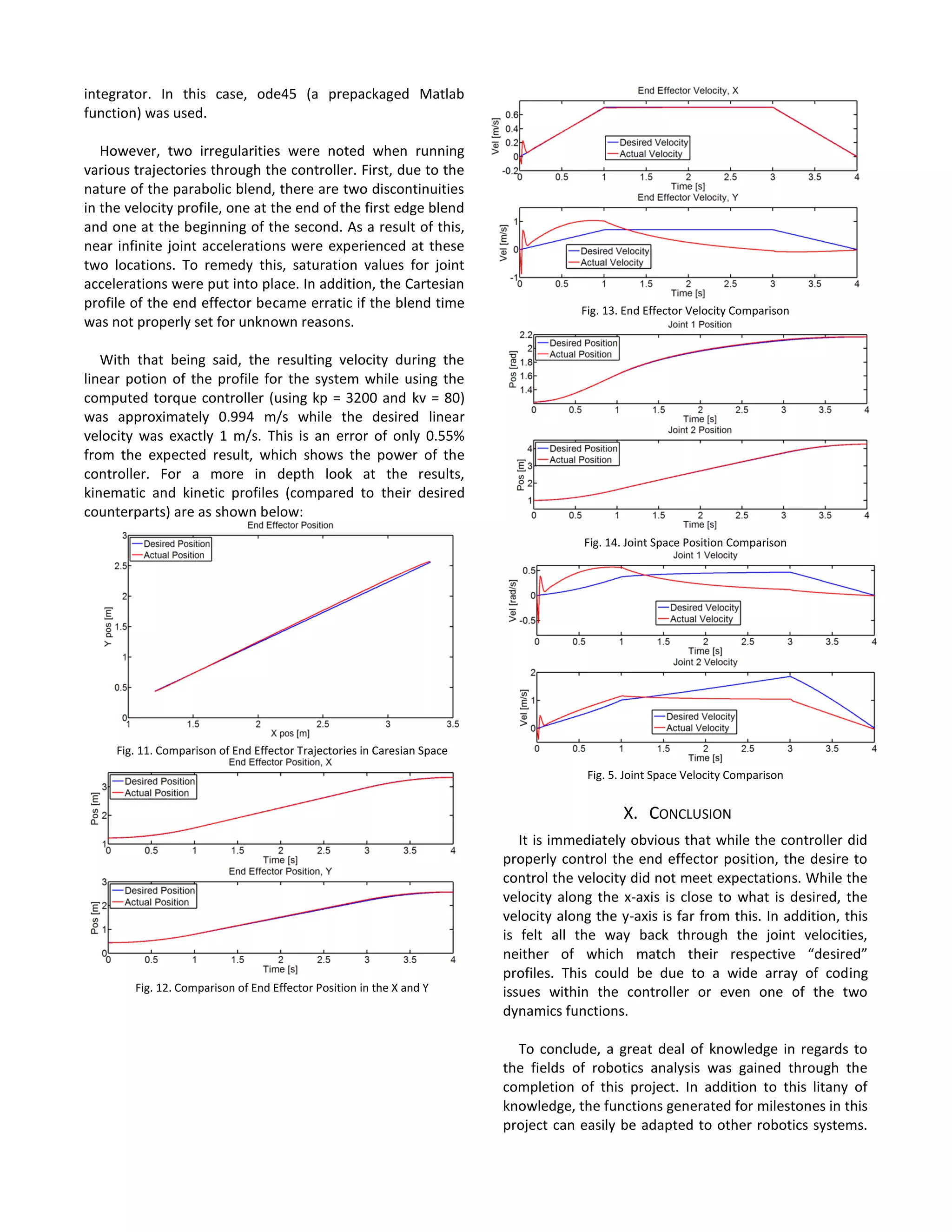
figure(1)
plot(x_des,y_des,'blue')
hold
plot(x_act,y_act, 'red')
title('End Effector Position')
ylabel('Y pos [m]')
xlabel('X pos [m]')
legend('Desired Position','Actual Position','location', 'northwest')
figure(2)
subplot(2,1,1)
plot(time,x_dot_des,'blue')
hold
plot(time,x_dot_act(1:400),'red')
title('End Effector Velocity, X')
ylabel('Vel [m/s]')
xlabel('Time [s]')
legend('Desired Velocity','Actual Velocity','location', 'northwest')
subplot(2,1,2)
plot(time,y_dot_des,'blue')
hold
plot(time,y_dot_act(1:400),'red')
title('End Effector Velocity, Y')
ylabel('Vel [m/s]')
xlabel('Time [s]')
legend('Desired Velocity','Actual Velocity','location', 'northwest')
figure(3)
subplot(2,1,1)
plot(time,g_amma_dot_des,'blue')
hold
plot(time,g_amma_dot_act(1:400),'red')
title('Joint 1 Velocity')
ylabel('Vel [rad/s]')
xlabel('Time [s]')
legend('Desired Velocity','Actual Velocity','location', 'northwest')
subplot(2,1,2)
plot(time,d_dot_des,'blue')
hold
plot(time,d_dot_act(1:400),'red')
title('Joint 2 Velocity')
ylabel('Vel [m/s]')
xlabel('Time [s]')
legend('Desired Velocity','Actual Velocity','location', 'northwest')
figure(4)
subplot(2,1,1)
plot(time,x_des,'blue')
hold
plot(time,x_act(1:400),'red')
title('End Effector Position, X')
ylabel('Pos [m]')
xlabel('Time [s]')
legend('Desired Position','Actual Position','location', 'northwest')
subplot(2,1,2)
plot(time,y_des,'blue')
hold
plot(time,y_act(1:400),'red')
title('End Effector Position, Y')
ylabel('Pos [m]')
xlabel('Time [s]')
legend('Desired Position','Actual Position','location', 'northwest')
figure(5)
subplot(2,1,1)
plot(time,g_amma_des,'blue')
hold
plot(time,g_amma_act(1:400),'red')
title('Joint 1 Position')
ylabel('Pos [rad]')
xlabel('Time [s]')
legend('Desired Position','Actual Position','location', 'northwest')
subplot(2,1,2)
plot(time,d_des,'blue')
hold
plot(time,d_act(1:400),'red')
title('Joint 2 Position')
ylabel('Pos [m]')
xlabel('Time [s]')
legend('Desired Position','Actual Position','location', 'northwest')
function qnew = forward_dynamics_control(t,q)
%Forward Dynamics
% INPUTS: q (current position of the robot), q_dot (current velocities), tau
(current
%generalized forces, time_period (time period for simulation)
% OUTPUTS: q_new (predicted position)
% q_dot_new (predicted velocities)
%Establish Global Variables
global a eta M1 M2 L1 L2 I1 I2 g
a1 = a*cos(eta);
a2 = a*sin(eta);
qnew = zeros(4,1);
%From the state model definition, p(2) & p(4) are the derivatives of
%p(1) & p(3), respectively
qnew(1) = q(2);
qnew(3) = q(4);
tau(1) = q(5);
tau(2) = q(6);

15. %Calculate components of the Mass matrix
m1 = M1*(0.25*a^2)+M2*(L2^2-
2*L2*(a+q(3))+a^2+2*a1*q(3)+q(3)^2)+I1+I2;
m2 = -M2*a2;
m3 = -M2*a2;
m4 = M2;
%Caculate components of the Force vector
v1 = 2*M2*(a1+q(3)-L2)*q(2)*q(4);
v2 = -M2*(a1+q(3)-L2)*q(2)^2;
g1 = (M1*L1*cos(-q(1))+M1*a*(sin(eta-q(1))*(sin(eta)-
sin(q(1))))+M2*cos(eta-q(1))*(a1-q(3)+L2)+M2*a2*sin(eta-q(1)))*g;
g2 = M2*g*sin(q(1)-eta);
%Initialize Mass Matrix and Force vector
m = [m1 m2; m3 m4];
F = [v1+g1+tau(1); v2+g2+tau(2)];
%Using the Mass Matrix and Force vector, determine pdot(2) &pdot(4)
%which are the angular acceleration of q and alpha, respectively
acc= m^(-1)*F;
qnew(2) = acc(1,1);
qnew(4) = acc(2,1);
qnew(5) = 0;
qnew(6) = 0;
end
B. Full Size Dynamics Matrices
𝑚(𝜃̈)
= [ 𝑚1 (
1
4
𝑎2
) + 𝑚2(𝐿2
2
− 2𝐿2(𝑎 + 𝑑) + 𝑎2
+ 2𝑎1 𝑑 + 𝑑2) + 𝐼1 + 𝐼2 −𝑚2 𝑎2
−𝑚2 𝑎2 𝑚2
]
(31)
𝑣(𝜃, 𝜃̇) = [
2𝑚2(𝑎1 + 𝑑 − 𝐿2)𝑑̇ 𝛾̇
−𝑚2(𝑎1 + 𝑑 + 𝐿2)𝛾̇2
] (32)
𝑔(𝜃)
= [
𝑚1 𝐿1 cos(−𝛾) + 𝑚1 𝑎(sin(𝜂 − 𝛾) (sin(𝜂) − sin(𝛾))) + 𝑚2 cos(𝜂 − 𝛾) (𝑎1 − 𝑑 + 𝐿2) + 𝑚2 𝑎2sin⁡( 𝜂 − 𝛾)
𝑚2sin⁡( 𝛾 − 𝜂)
]