Learning Objectives
- Understandlinear regression
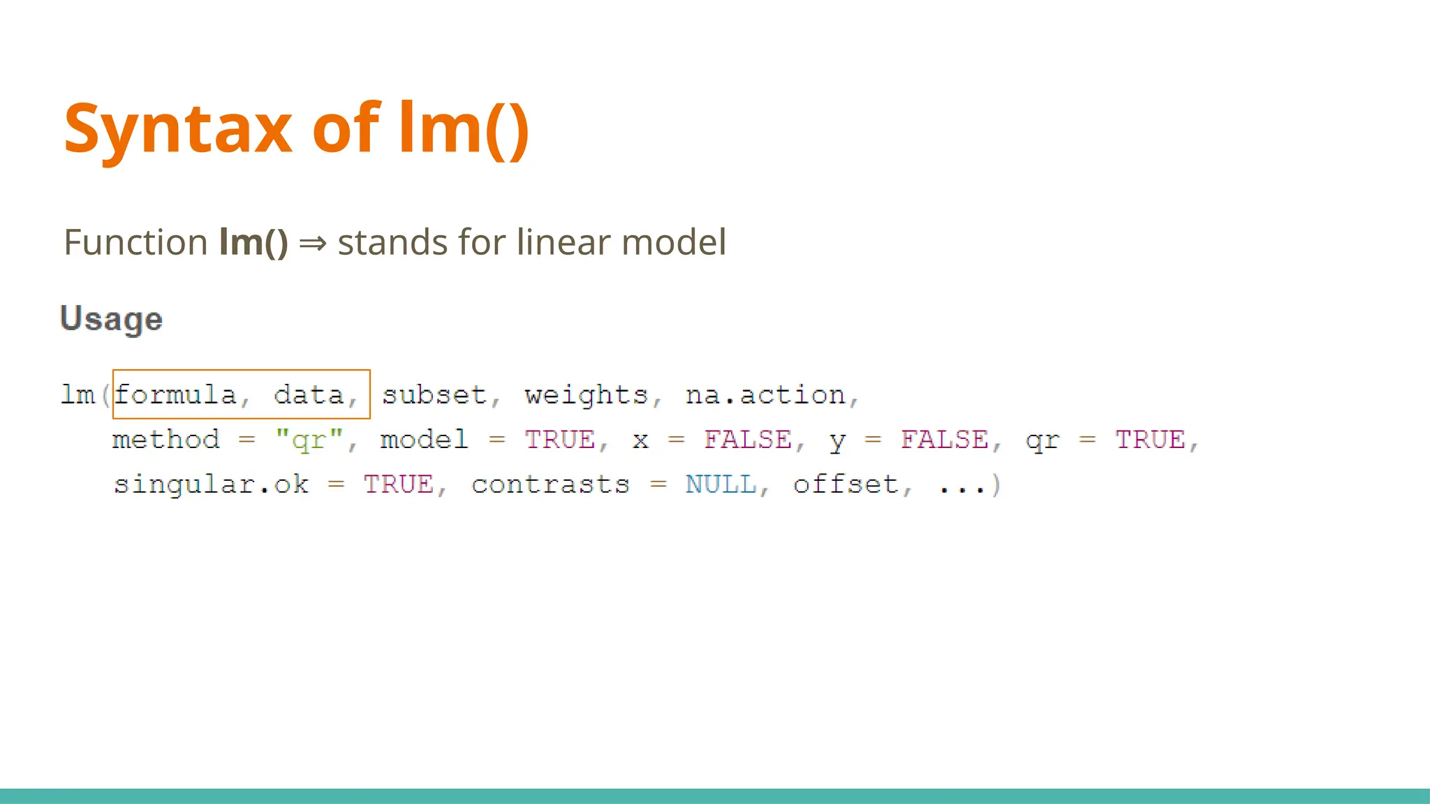
- Understand purpose of lm() function
- Using lm() to fit regression models
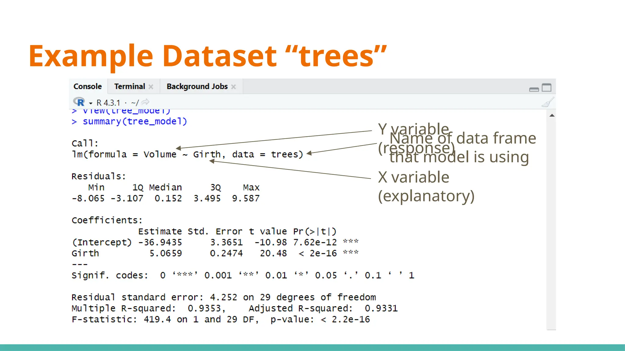
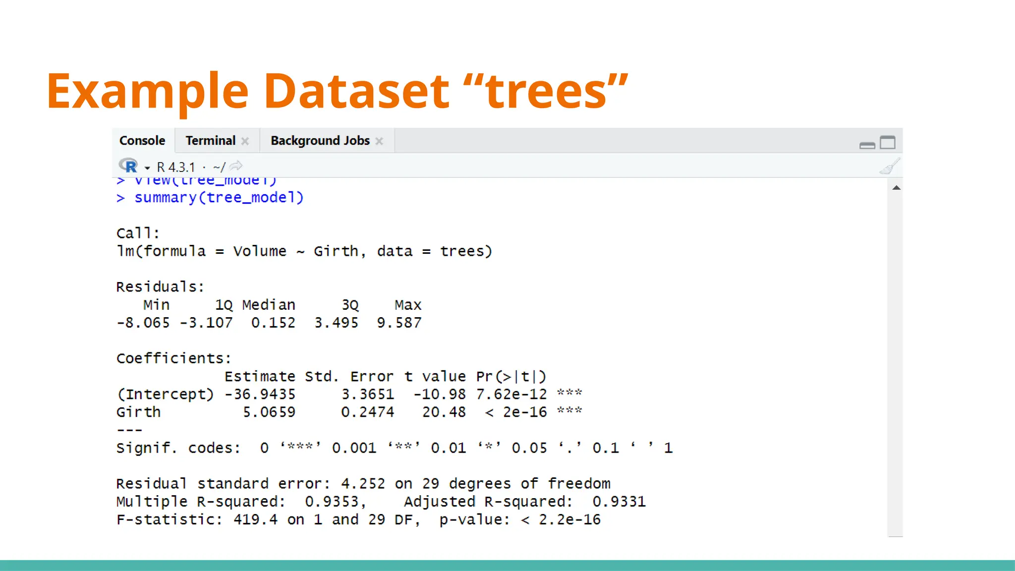
- Interpret output of lm() function
3.
Ever Wondered How…
-Maps are able to estimate your travelling time
- Surcharge pricing are determined to meet
demands for taxi
- HDB resale prices are forecasted
4.
What is LinearRegression?
- Interested in the relationship between a dependent variable (y)
and one or more independent variables (x)
- Models relationships between variables
- Simple Linear Regression (1 independent variable)
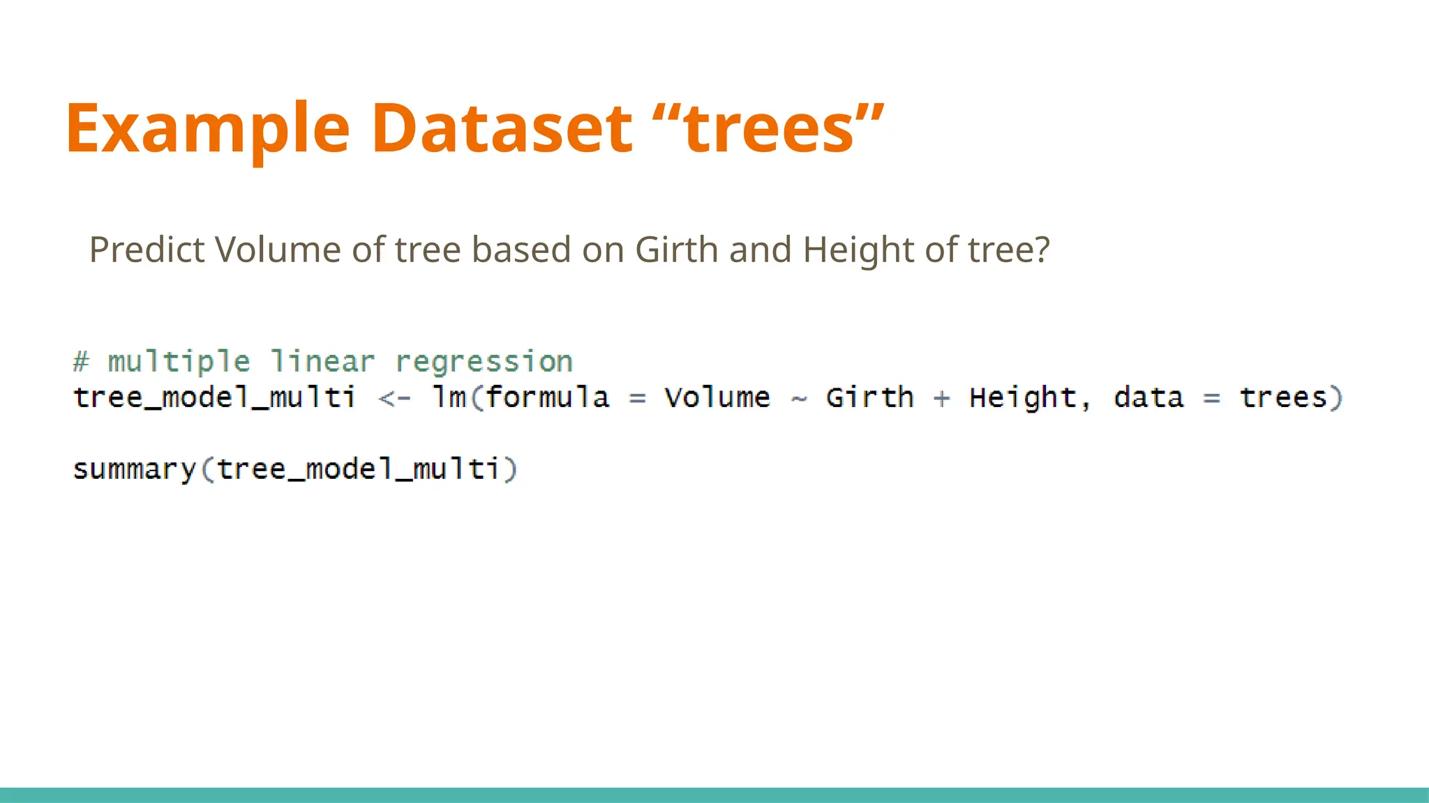
- Multiple Linear Regression (2 or more independent variables)
- Finds best-fit line that minimises distance between observed
data values and predicted values
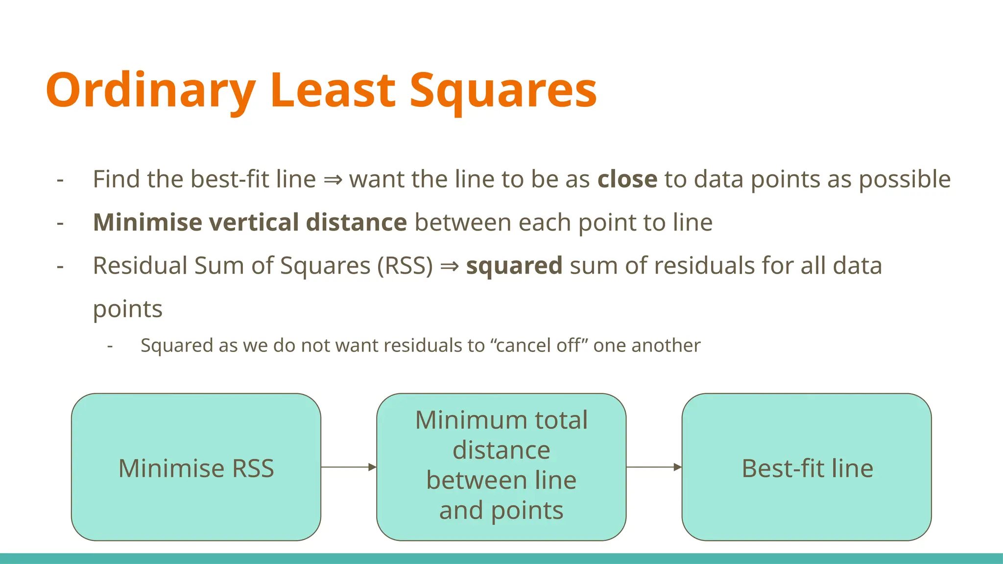
Ordinary Least Squares
-Find the best-fit line want the line to be as
⇒ close to data points as possible
- Minimise vertical distance between each point to line
- Residual Sum of Squares (RSS) ⇒ squared sum of residuals for all data
points
- Squared as we do not want residuals to “cancel off” one another
Minimise RSS
Minimum total
distance
between line
and points
Best-fit line
7.
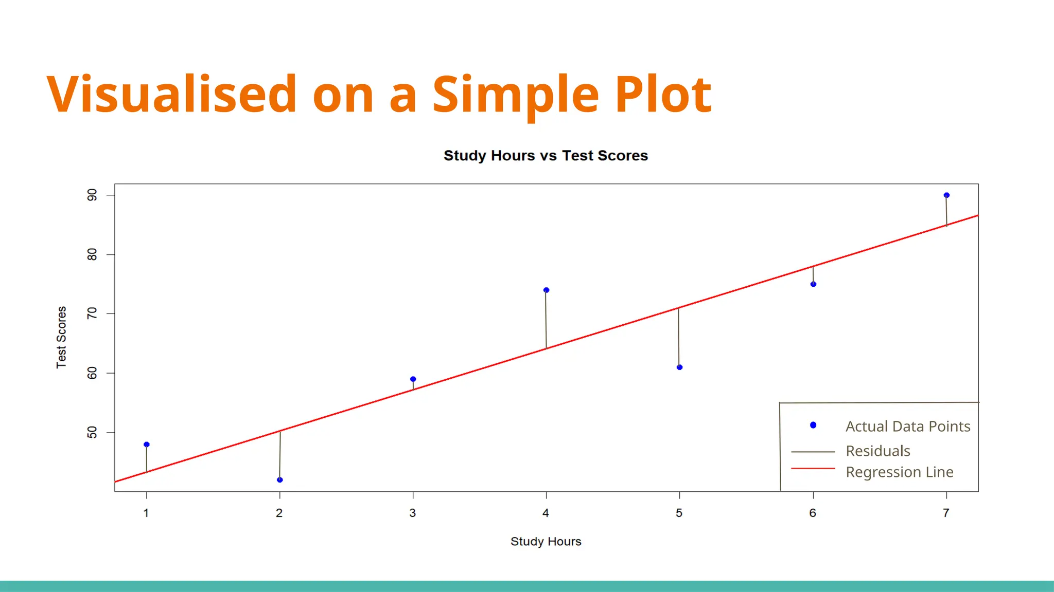
Visualised on aSimple Plot
Actual Data Points
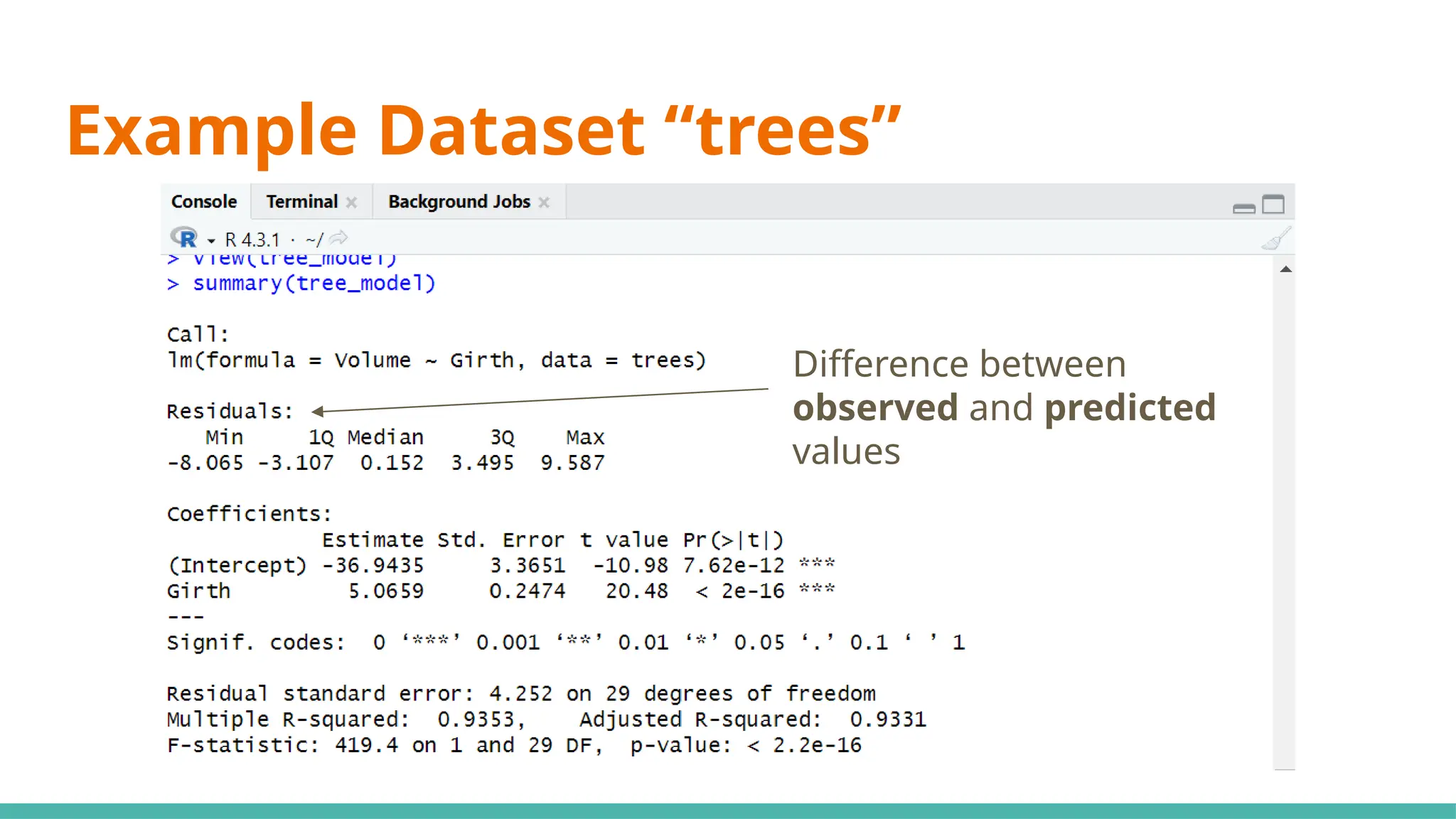
Residuals
Regression Line
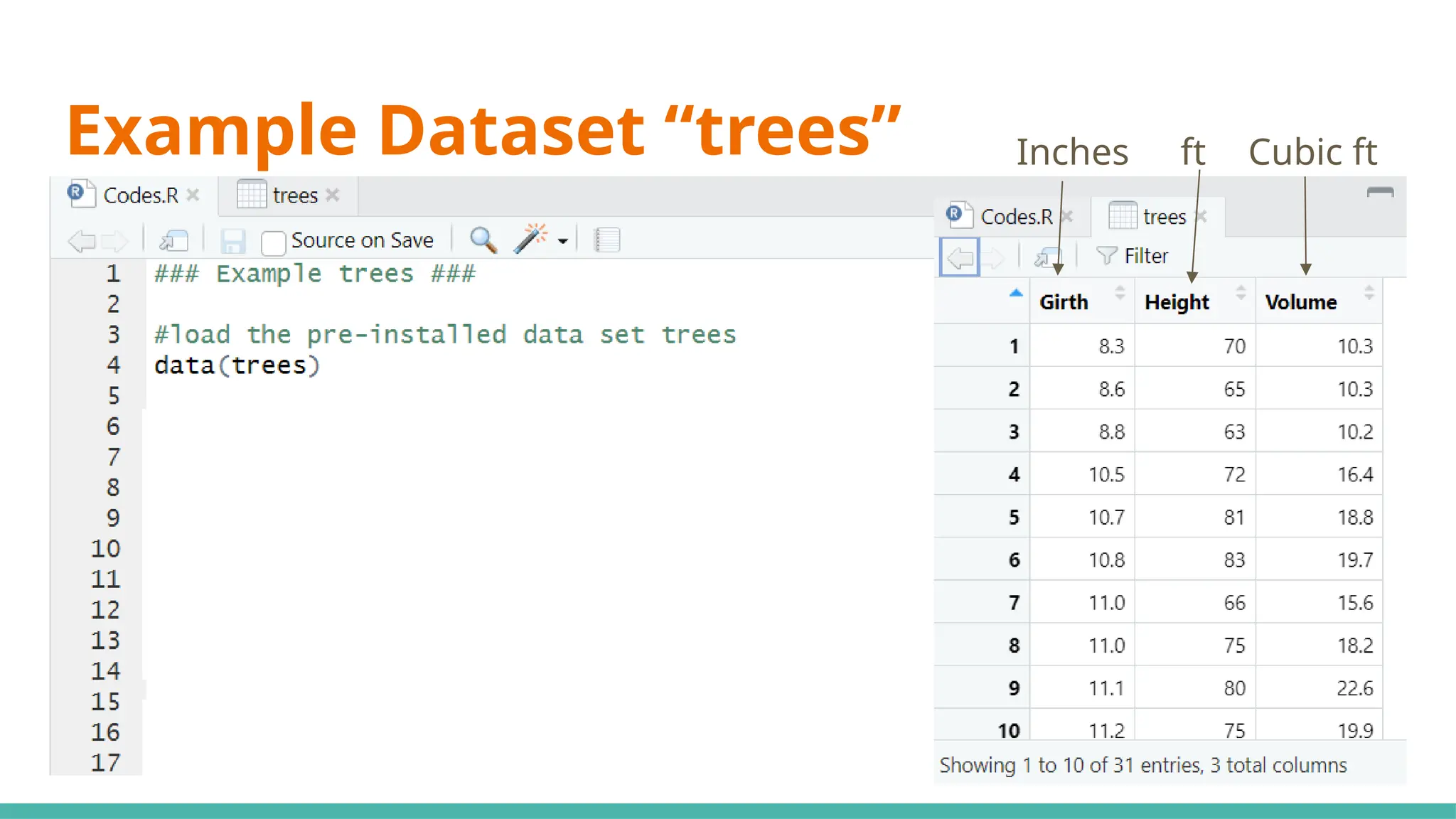
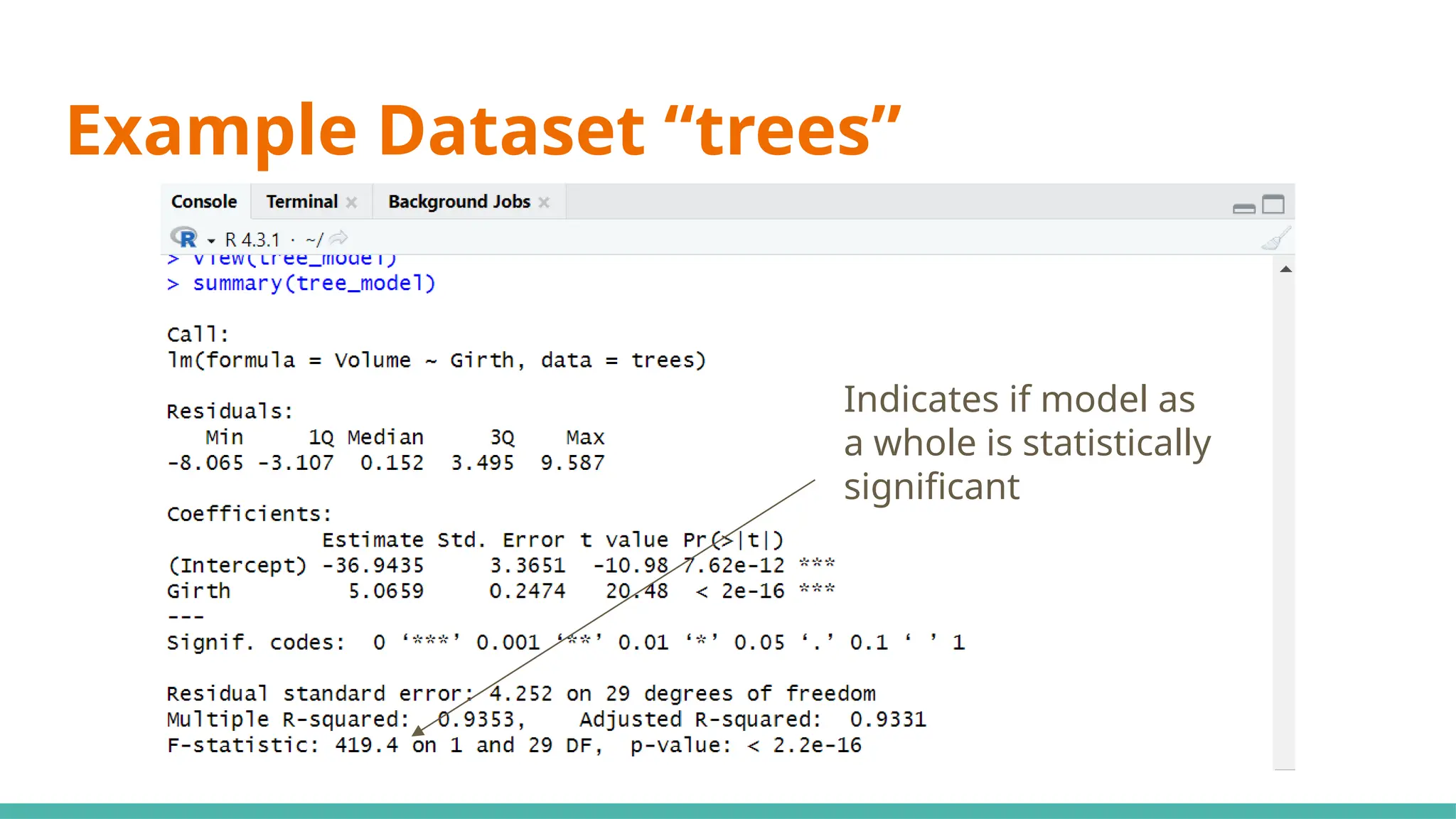
#10 Simple linear regression (SLR) (black cherry trees)
#13 Min ⇒ represents the data point furthest below the regression line
1Q ⇒ 25% of the residuals are less than this number
3Q ⇒ 25% of teh residuals are greater than this number
Max ⇒ point that is furthest from the regression line
Mean of residuals not shown as it will always be 0
Now, what can we infer just from the residuals alone to determine if this can be a good linear regression model?
Median of residuals ideally should be as close to 0 as possible (hard to preface what is close or far as it is relative to your data)
Why ⇒ this would imply our model isnt skewed one way or another
Another would be that it is symmetrically distributed ⇒ want min and max to have same magnitude, as well as 1Q and 3Q
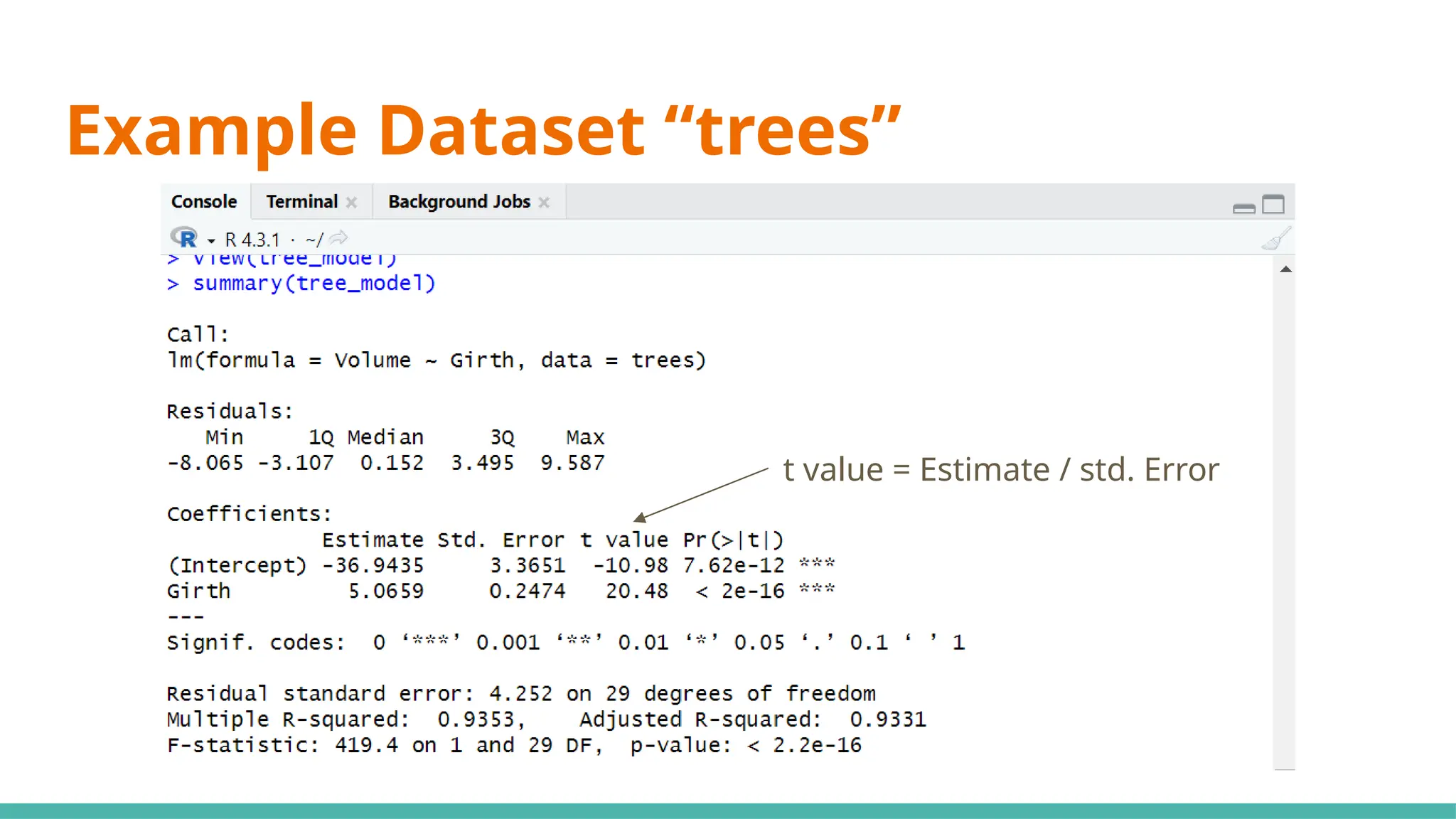
#15 Moving on to coefficients, the intercept will always be given, including any x variables that we have provided ⇒ y=mx+c
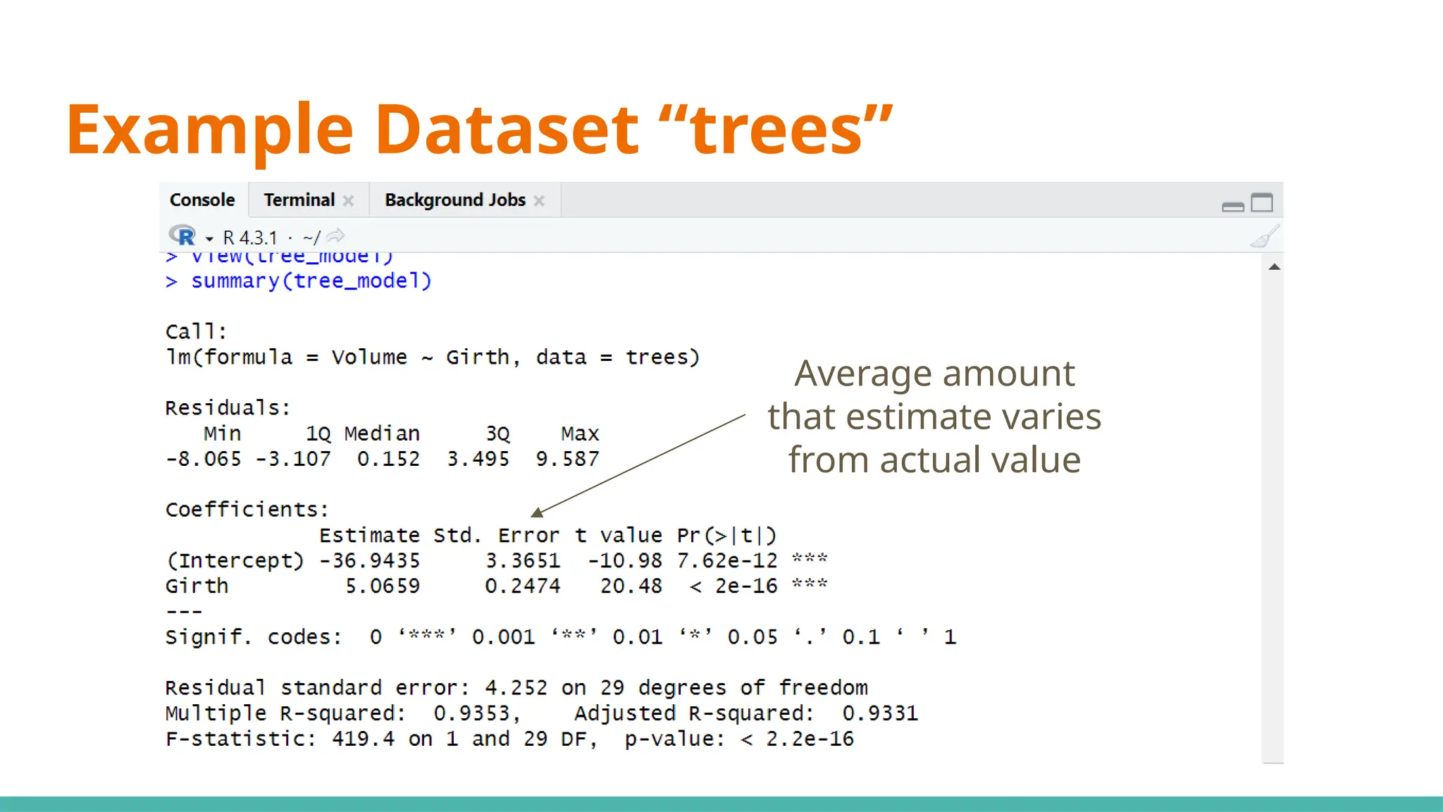
#17 Standard error ⇒ responsible for the width of the confidence interval
Ideally, you want a lower number relative to the estimate for standard error (e.g. standard error is small compared to est)
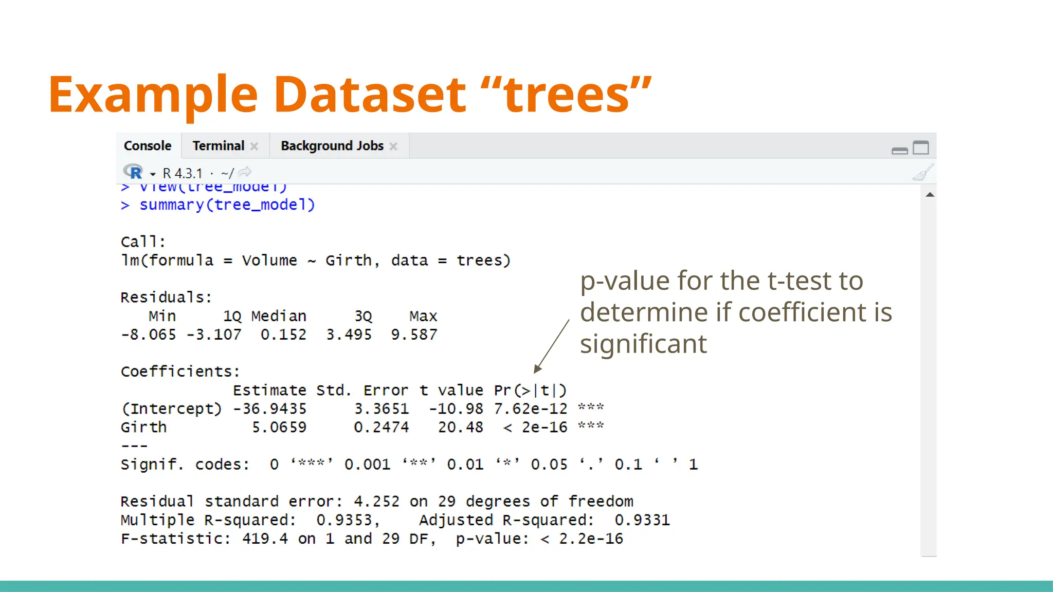
#21 We use 0.05 as a benchmark, it means that it is unlikely that the relationship between the y variable and x variable is due to chance ⇒ statistically significant
Stars on the right shows the significant levels, as seen in the significant codes
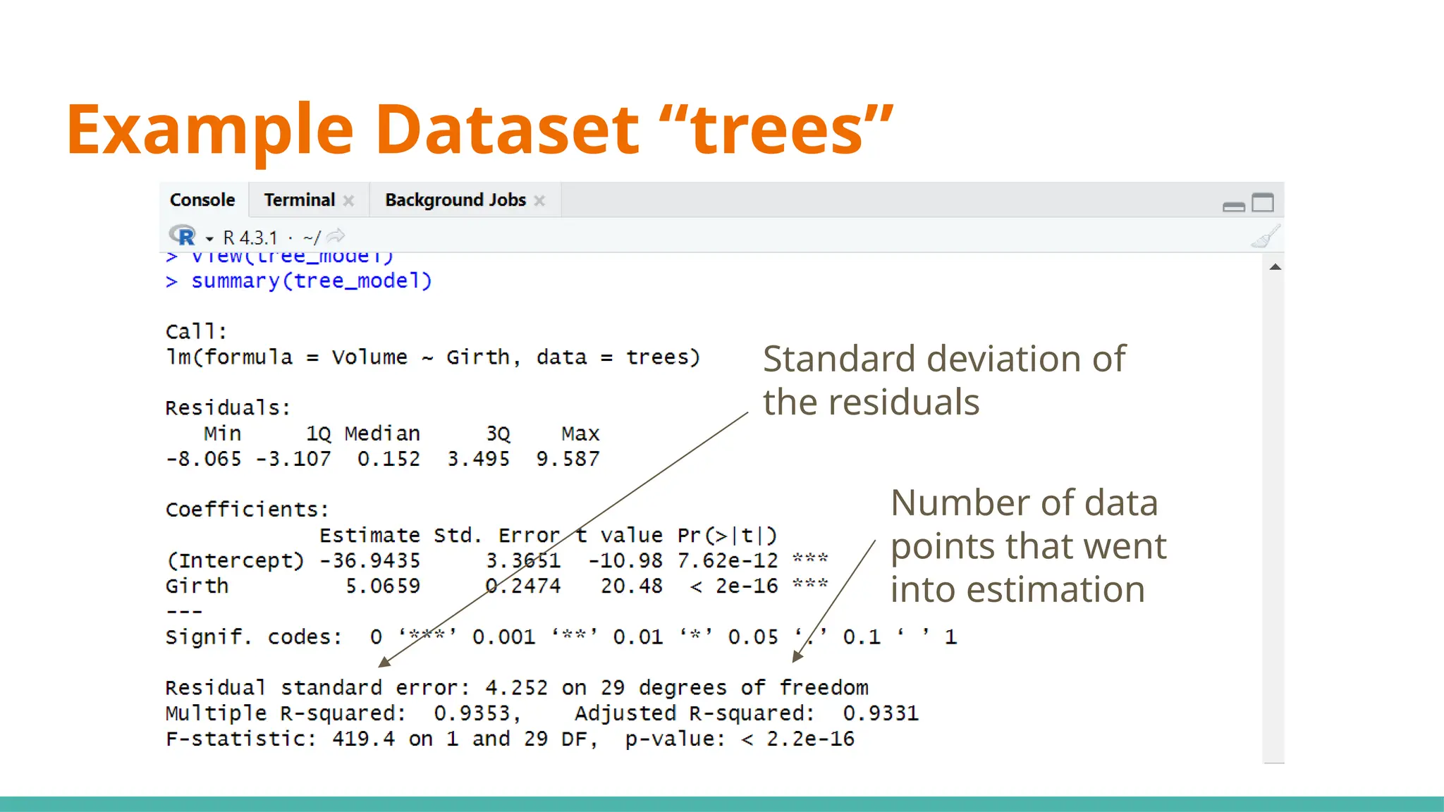
#23 Standard deviation of residuals ⇒ average distance of points from the regression line, adjusted with the number of points
Degrees of freedom ⇒ number of observations (31) minus number of variables (29)
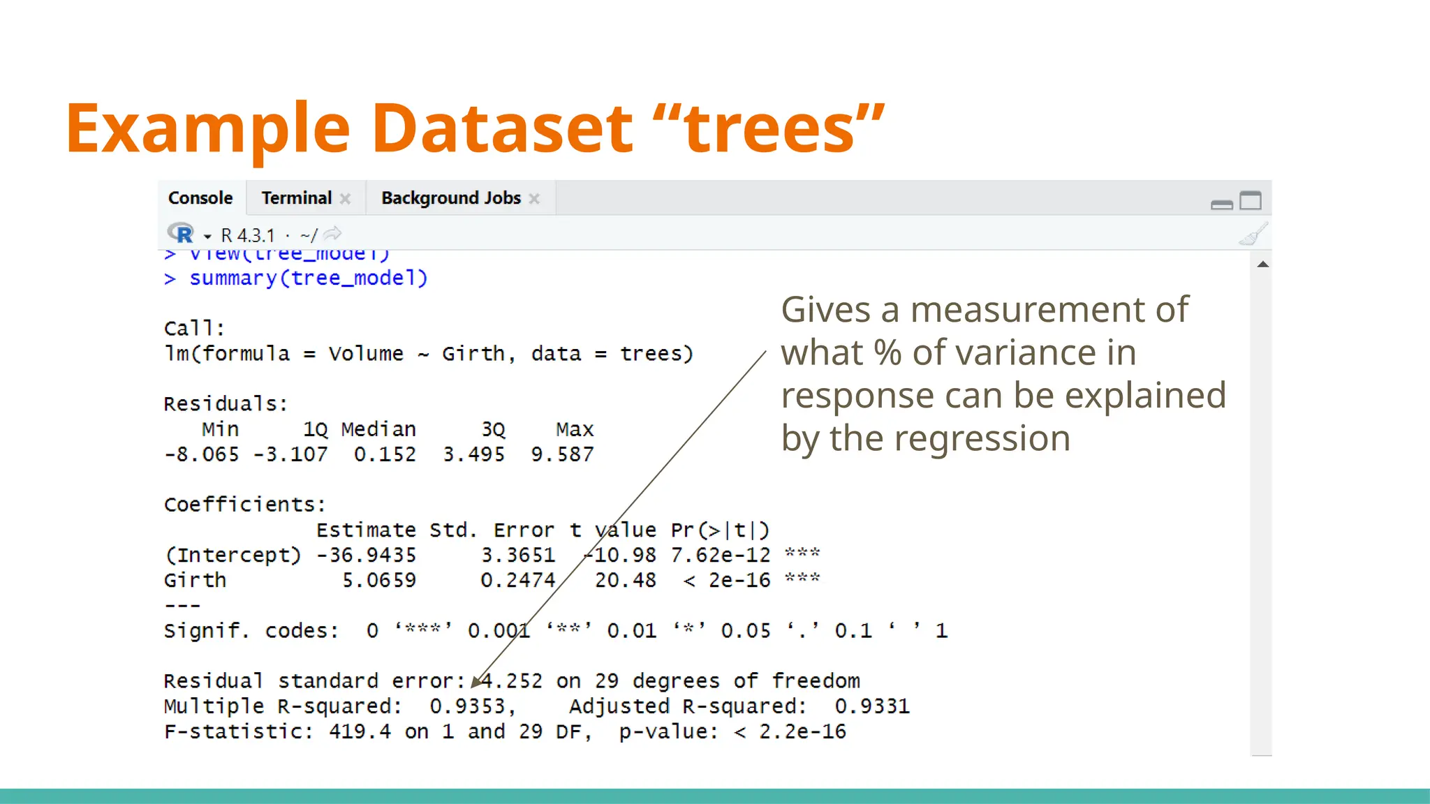
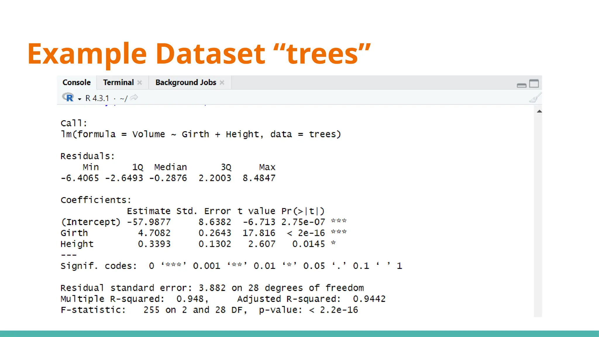
#25 Multiple R-squared ⇒ Generally gets better with more x variables
Adjusted R-squared ⇒ Penalises for adding useless predictor (x) variables
If multi R-squared is much higher than your adjusted, your model might be overfitted
#27 Want a value way bigger than 1 to be statistically significant, or you can just refer to p-value where if it is <0.05 it would be significant