This document provides an overview of mathematical functions in MATLAB, including: 1) Common math functions such as absolute value, rounding, floor/ceiling, exponents, logs, and trigonometric functions. 2) How to write custom functions and use programming constructs like if/else statements and for loops. 3) Data analysis functions including statistics and histograms. 4) Complex number representation and basic complex functions in MATLAB.

1. ECE 1010 ECE Problem Solving I
MATLAB 3
Functions
Overview
In this chapter we start studying the many, many, mathematical
functions that are included in MATLAB. Some time will be spent
introducing complex variables and how MATLAB handles them.
Later we will learn how to write custom (user written) functions
which are a special form of m-file. Two dimensional plotting
functions will be introduced. We will also explore programming
constructs for flow control (if-else-elseif code blocks)
and looping (for loop etc.). Next data analysis functions will be
investigated, which includes sample statistics and histogram plot-
ting functions.
Chapter 3: Overview 3–1

2. ECE 1010 ECE Problem Solving I
Mathematical Functions
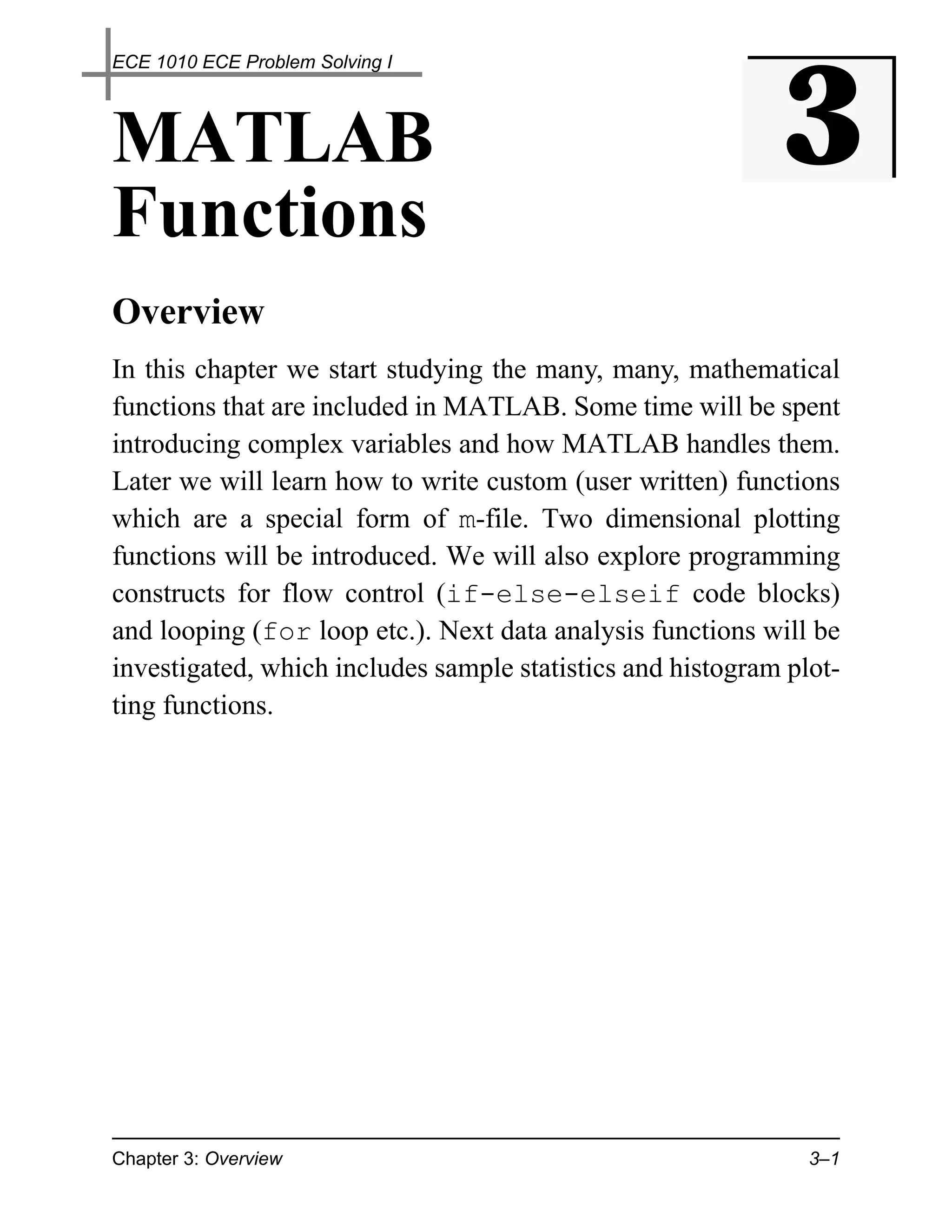
Common Math Functions
Table 3.1: Common math functions
Function Description Function Description
abs(x) x sqrt(x) x
round(x) nearest integer fix(x) nearest integer
floor(x) nearest integer ceil(x) nearest integer
toward – ∞ toward ∞
sign(x) rem(x,y) the remainder
 – 1, x < 0
 of x ⁄ y
 0, x = 0

 1, x > 0
exp(x) x log(x) natural log ln x
e
log10(x) log base 10
log 10 x
Examples:
» x = [-5.5 5.5];
» round(x)
ans = -6 6
» fix(x)
ans = -5 5
» floor(x)
ans = -6 5
» ceil(x)
Chapter 3: Mathematical Functions 3–2

3. ECE 1010 ECE Problem Solving I
ans = -5 6
» sign(x)
ans = -1 1
» rem(23,6)
ans = 5
Trigonometric and Hyperbolic Functions
• Unlike pocket calculators, the trigonometric functions always
assume the input argument is in radians
• The inverse trigonometric functions produce outputs that are
in radians
Table 3.2: Trigonometric functions
Function Description Function Description
sin(x) sin ( x ) cos(x) cos ( x )
tan(x) tan ( x ) asin(x) –1
sin ( x )
acos(x) –1 atan(x) –1
cos ( x ) tan ( x )
atan2(y, the inverse tan-
x) gent of y ⁄ x
including the
correct quad-
rant
Examples:
2 2
• A simple verification that sin ( x ) + cos ( x ) = 1
Chapter 3: Mathematical Functions 3–3

4. ECE 1010 ECE Problem Solving I
» x = 0:pi/10:pi;
» [x' sin(x)' cos(x)' (sin(x).^2+cos(x).^2)']
ans =
0 0 1.0000 1.0000
0.3142 0.3090 0.9511 1.0000
0.6283 0.5878 0.8090 1.0000
0.9425 0.8090 0.5878 1.0000
1.2566 0.9511 0.3090 1.0000
1.5708 1.0000 0.0000 1.0000
1.8850 0.9511 -0.3090 1.0000
2.1991 0.8090 -0.5878 1.0000
2.5133 0.5878 -0.8090 1.0000
2.8274 0.3090 -0.9511 1.0000
3.1416 0.0000 -1.0000 1.0000
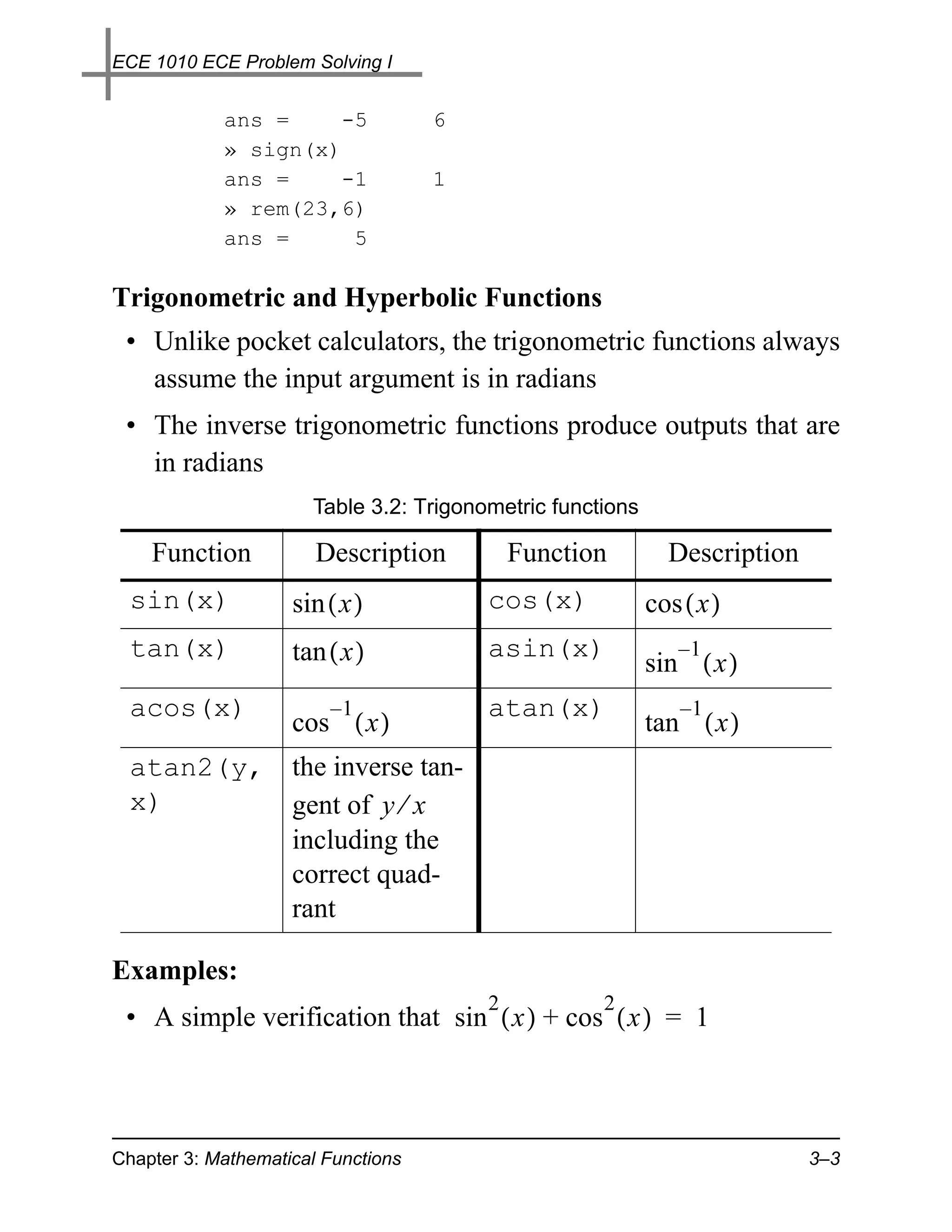
• Parametric plotting:
– Verify that by plotting sin θ versus cos θ for 0 ≤ θ ≤ 2π we
obtain a circle
» theta = 0:2*pi/100:2*pi; % Span 0 to 2pi with 100 pts
» plot(cos(theta),sin(theta)); axis('square')
» title('Parametric Plotting','fontsize',18)
» ylabel('y - axis','fontsize',14)
» xlabel('x - axis','fontsize',14)
» figure(2)
» hold
Current plot held
» plot(cos(5*theta).*cos(theta), ...
cos(5*theta).*sin(theta)); % A five-leaved rose
Chapter 3: Mathematical Functions 3–4

5. ECE 1010 ECE Problem Solving I
Parametric Plotting
1
Circle
0.8
0.6
0.4 Rose
0.2
y - axis
0
-0.2
-0.4
-0.6
-0.8
-1
-1 -0.8 -0.6 -0.4 -0.2 0 0.2 0.4 0.6 0.8 1
x - axis
• The trig functions are what you would expect, except the fea-
tures of atan2(y,x) may be unfamiliar
y y
4
2 x 2 x
φ 1 = 0.4636
4
φ 2 = – 2.0344
Chapter 3: Mathematical Functions 3–5

6. ECE 1010 ECE Problem Solving I
» [atan(2/4) atan2(2,4)]
ans = 0.4636 0.4636 % the same
» [atan(-4/-2) atan2(-4,-2)]
ans = 1.1071 -2.0344 % different; why?
x
• The hyperbolic functions are defined in terms of e
Table 3.3: Hyperbolic functions
Function Description Function Description
sinh(x) x –x cosh(x) x –x
e –e e –e
-----------------
- -----------------
-
2 2
tanh(x) x –x asinh(x) 2
e –e
------------------ ln ( x + x + 1 )
x –x
e +e
acosh(x) 2 atanh(x) 1+x
ln ( x + x – 1 ) ln -----------, x ≤ 1
-
1–x
• There are no special concerns in the use of these functions
except that atanh requires an argument that must not
exceed an absolute value of one
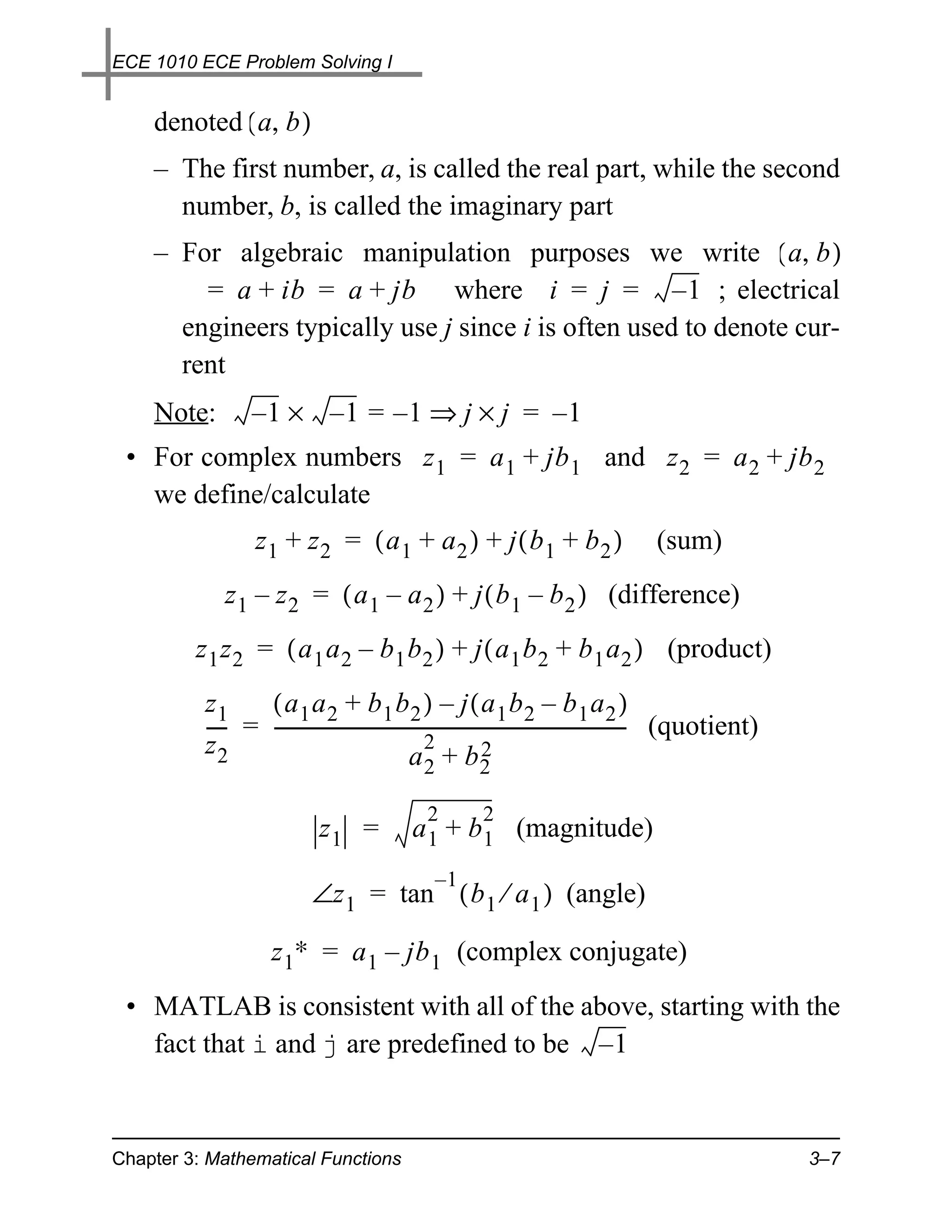
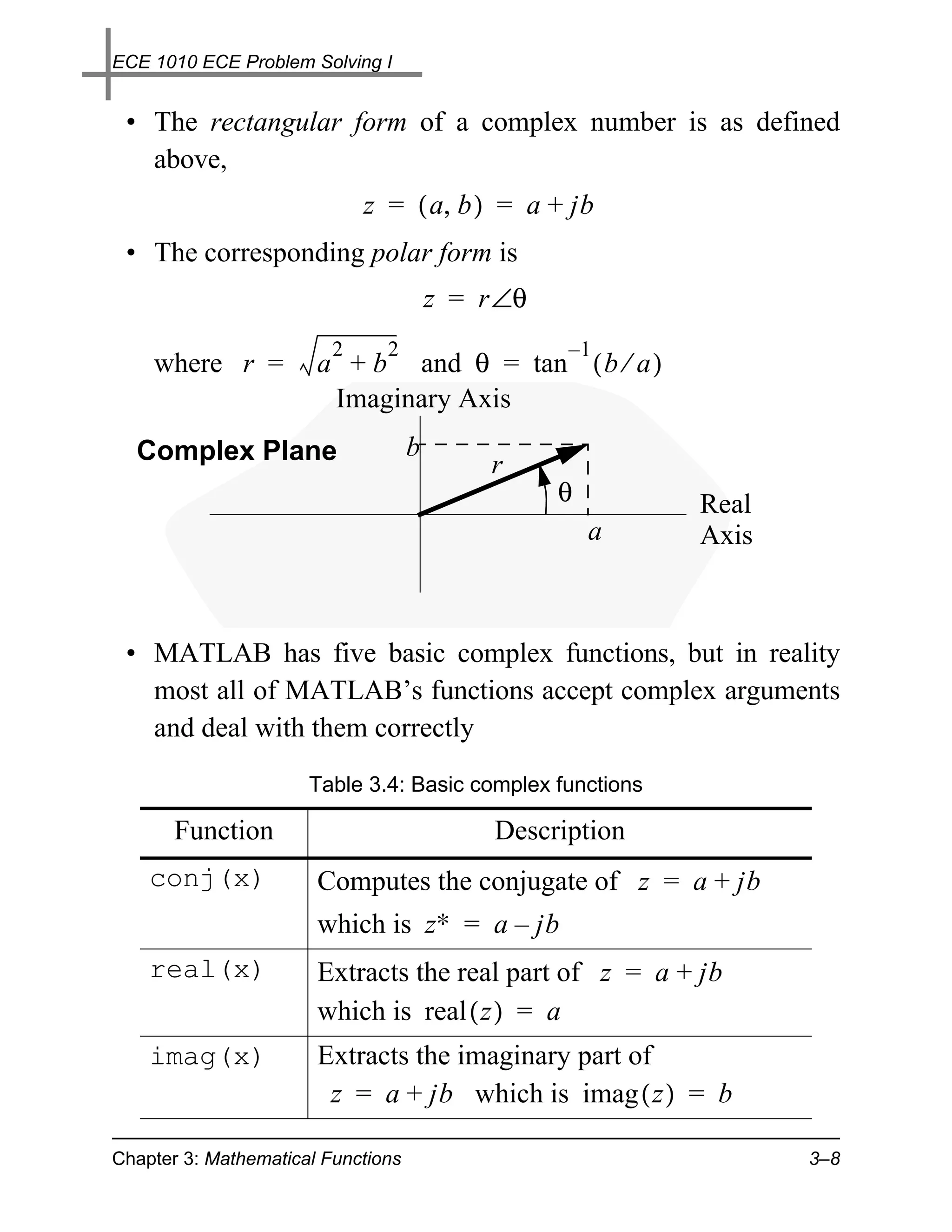
Complex Number Functions
• Before discussing these functions we first review a few facts
about complex variable theory
• In electrical engineering complex numbers appear frequently
• A complex number is an ordered pair of real numbers1
1. Tom M. Apostle, Mathematical Analysis, second edition, Addison Wesley,
p. 15, 1974.
Chapter 3: Mathematical Functions 3–6

7. ECE 1010 ECE Problem Solving I
denoted ( a, b )
– The first number, a, is called the real part, while the second
number, b, is called the imaginary part
– For algebraic manipulation purposes we write ( a, b )
= a + ib = a + jb where i = j = – 1 ; electrical
engineers typically use j since i is often used to denote cur-
rent
Note: –1 × –1 = –1 ⇒ j × j = –1
• For complex numbers z 1 = a 1 + jb 1 and z 2 = a 2 + jb 2
we define/calculate
z1 + z2 = ( a1 + a2 ) + j ( b1 + b2 ) (sum)
z 1 – z 2 = ( a 1 – a 2 ) + j ( b 1 – b 2 ) (difference)
z 1 z 2 = ( a 1 a 2 – b 1 b 2 ) + j ( a 1 b 2 + b 1 a 2 ) (product)
z1 ( a1 a2 + b1 b2 ) – j ( a1 b2 – b1 a2 )
---- = --------------------------------------------------------------------------- (quotient)
-
z2 2 2
a +b
2 2
2 2
z1 = a 1 + b 1 (magnitude)
–1
∠z 1 = tan ( b 1 ⁄ a 1 ) (angle)
z 1∗ = a 1 – jb 1 (complex conjugate)
• MATLAB is consistent with all of the above, starting with the
fact that i and j are predefined to be – 1
Chapter 3: Mathematical Functions 3–7

8. ECE 1010 ECE Problem Solving I
• The rectangular form of a complex number is as defined
above,
z = ( a, b ) = a + jb
• The corresponding polar form is
z = r ∠θ
2 2 –1
where r = a + b and θ = tan ( b ⁄ a )
Imaginary Axis
Complex Plane b
r
θ Real
a Axis
• MATLAB has five basic complex functions, but in reality
most all of MATLAB’s functions accept complex arguments
and deal with them correctly
Table 3.4: Basic complex functions
Function Description
conj(x) Computes the conjugate of z = a + jb
which is z∗ = a – jb
real(x) Extracts the real part of z = a + jb
which is real ( z ) = a
imag(x) Extracts the imaginary part of
z = a + jb which is imag ( z ) = b
Chapter 3: Mathematical Functions 3–8

9. ECE 1010 ECE Problem Solving I
Table 3.4: Basic complex functions
Function Description
angle(x) computes the angle of z = a + jb using
atan2 which is
atan2(imag(z),real(z))
Euler’s Formula: A special mathematical result of, special
importance to electrical engineers, is the fact that
jb
e = cos b + j sin b (3.1)
• Turning (3.1) around yields
jθ – jθ
e –e
sin θ = ---------------------
- (3.2)
2j
jθ – jθ
e +e
cos θ = ---------------------
- (3.3)
2
• It also follows that
jθ
z = a + jb = re (3.4)
where
2 2 –1 b
r= a + b , θ = tan --, a = r cos θ, b = r sin θ
-
a
Chapter 3: Mathematical Functions 3–9

10. ECE 1010 ECE Problem Solving I
• Some examples:
» z1 = 2+j*4; z2 = -5+j*7;
» [z1 z2]
ans =
2.0000 + 4.0000i -5.0000 + 7.0000i
» [real(z1) imag(z1) abs(z1) angle(z1)]
ans =
2.0000 4.0000 4.4721 1.1071
» [conj(z1) conj(z2)]
ans =
2.0000 - 4.0000i -5.0000 - 7.0000i
» [z1+z2 z1-z2 z1*z2 z1/z2]
ans =
-3.0000 +11.0000i 7.0000 - 3.0000i
-38.0000 - 6.0000i 0.2432 - 0.4595i
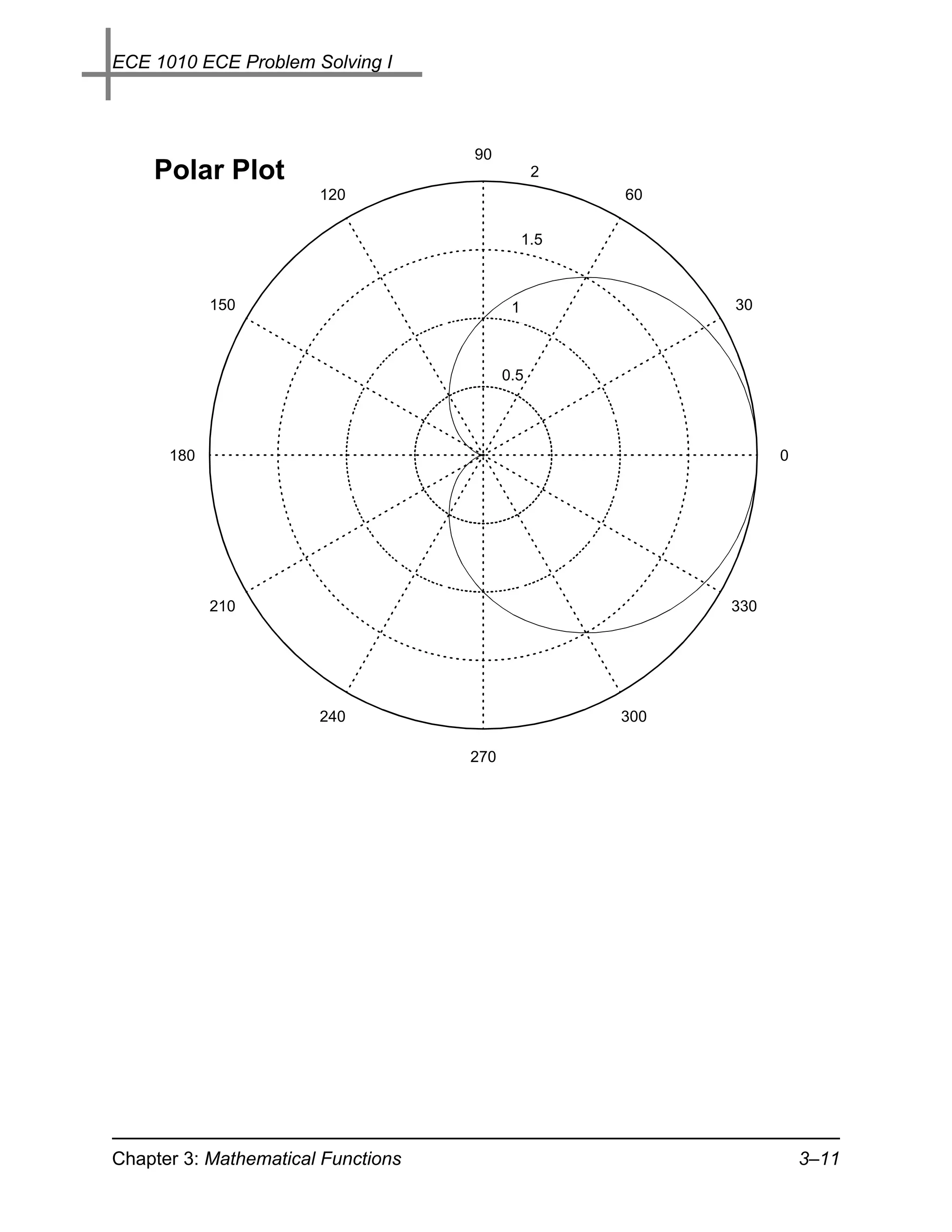
Polar Plots: When dealing with complex numbers we often deal
with the polar form. The plot command which directly plots vec-
tors of magnitude and angle is polar(theta,r)
• This function is also useful for general plotting
• As an example the equation of a cardioid in polar form, with
parameter a, is
r = a ( 1 + cos θ ), 0 ≤ θ ≤ 2π
» theta = 0:2*pi/100:2*pi; % Span 0 to 2pi with 100 pts
» r = 1+cos(theta);
» polar(theta,r)
Chapter 3: Mathematical Functions 3–10

11. ECE 1010 ECE Problem Solving I
90
Polar Plot 2
120 60
1.5
150 1 30
0.5
180 0
210 330
240 300
270
Chapter 3: Mathematical Functions 3–11