This document discusses optimization problems involving a single variable. It begins by introducing optimization problems and defining key concepts like objective functions, constraints, and optimality conditions. It then presents methods for solving single variable optimization problems both analytically and numerically. Analytically, it discusses using derivatives to find maxima and minima, and classifying functions as unimodal, convex, or concave. Numerically, it describes bracketing methods to bound the solution and the Newton-Raphson method requiring derivatives. It also introduces the golden section search method, a region-elimination technique.

1. CHAPTER 7. OPTIMIZATION: SINGLE VARIABLE PROBLEMS
7.1 INTRODUCTION
Consider the following consecutive reactions A B C taking place
in a plug flow reactor. We are interested in finding the yield of the intermediate product
B. The yield is defined by where is the feed concentration of A. If we write
the mass balances for the species A and B, this yields:
⎯→⎯ 1k
⎯→⎯ 2k
oA
B
oA
Ak
d
dA
1−=
τ (7.1)
BkAk
d
dB
21 −=
τ (7.2)
These equations are combined to give:
A
B
k
k
dA
dB
1
2
1+−=
(7.3)
This differential equation can be integrated to give the yield B/A0
K
o
oK
o
C
A
B
CC
KA
B
+−
−
= )(
1
1
(7.4)
where
1
2
k
k
Kand
A
A
C
o
==
(7.5)
Now we would like to determine the conditions that would give the maximum value of
the yield of B. This type of problem is an optimization problem. An optimization
problem consists in finding the maximum or minimum of a function. The function is
called an objective function. In this example the objective function is to maximize the
yield of B as given by Eq.(7.4) It can be seen that the yield of B depends on three
variables (C, K, Bo/Ao). The optimization consists in finding the combination of these
1

2. variables that would give the maximum yield. In general the values K and Bo/Ao are
known. The only optimization variable is C and the problem is a single variable
optimization. If we look closely at the variable C we know that the concentration A has
to be always less than the feed concentration Ao. Therefore the acceptable value of C
has to be bounded by 0 and 1. This single variable optimization consists in finding the
value of C that maximizes Eq.(7.4) knowing that C is bounded by 0 and 1.
Now suppose that we want to find the values of C and also that of Bo/Ao that
maximize the yield of B. In this optimization problem the objective function is still the
same (find the maximum value of the yield) but the optimization variables are two: C
and Bo/Ao. This is a multivariable optimization variable. Note that C is still bounded by
0 and 1. So we say that it is a multivariable constrained problem. In general the
constraints are not only simple bounds but they can be explicit equations that arise
generally from different balance equations.
In general, then, the optimization of any process refers to finding the values of the
process parameters that maximize or minimize a certain criterion within the constraints
inherent in the process model. The criteria, also called the objective function, can
represent the profit, cost, energy or other practical criteria. Optimization embraces
therefore all the fields of science, engineering and business .
In the chemical engineering field, optimization is used to solve a wide variety of
problems in the design, construction and operation of a chemical process. Examples of
application of optimization include the evaluation of plant data to construct a model of a
process, equipment and plant design, operation and control of the plant, allocation of
resources among several processes etc. In this chapter we will present some numerical
techniques for the solution of the following classes of optimization problems:
• Single variable problems
• Multivariable unconstrained problems
• Multivariable constrained problems
2

3. 7-2 INTRODUCTION TO OPTIMIZATION OF ONE SINGLE VARIABLE
FUNCTION
A one-dimensional optimization problem has the following form:
)()maximize(minimize xfor
x
(7.6)
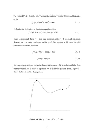
with
bxa ≤≤ (7.7)
That is, finding the optimum (maximum or minimum) of the objective function f(x) in
the region x∈ [a,b]. It should be useful to note that maximizing f(x) is equivalent to
minimizing −f(x).
The geometric characteristics of the objective function play an important role in
the solution of the optimization problem .Two important characteristics are discussed
below.
Figure 7-1: Unimodal function
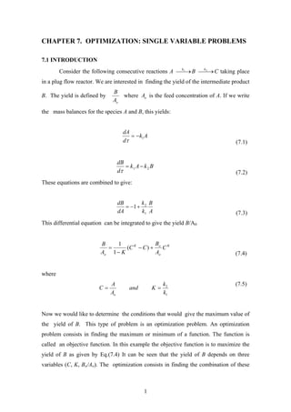
7.2.1 Unimodal Function
Figure 7-1 shows the plot of an objective function f(x). Over the interval [a,b]
the function has only one optimum (in this case a maximum). This function is called
unimodal. Multimodal functions, on the other hand, have more than one optimum.
3

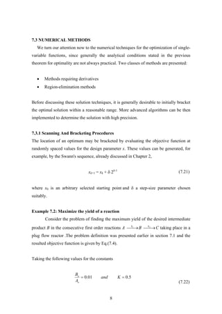
4. a b
x
f (x)
x1 x2
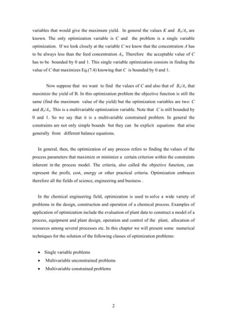
Figure 7-2: Multimodal function
7.2.2 Convex Functions
Another important property of the objective function is the convexity or
concavity. The one-single variable optimization problem is said to be convex (concave)
if the objective function is convex (concave) .The function f(x) is said to be convex over
a region R if the following inequality holds for two arbitrary values xa and xb in the
region R
(7.8))()1()())1(( baba xfxfxxf θ−+θ≤θ−+θ
Where θ is any scalar ∈ [0,1]. The sign of the inequality is replaced by ≥ for a concave
function. For the single variable function, the convexity can be characterized using the
second derivative of f(x). It can be shown that:
4

5. (7.9)convexisf(x)if0≥′′f
While
(7.10)concaveisf(x)if0≤′′f
Figure 7-3 and 7-4 show examples of convex and concave functions. The concept of
convexity is important in two aspects: It allows the use of appropriate and faster
optimization algorithms and it helps to determine whether the obtained optimum is a
local or global optimum. If a convex (or concave) function has a local optimum it is also
the global one.
Figure 7-3: Concave function Figure 7-4: Convex function
7.2.3 Optimality Conditions
Consider the objective function with a local maximum x*
shown in Figure 7-1. A
Taylor's expansion for a point x close to the assumed optimum x*
yields
(7.11)
L+′′′−+′′−+′−+= )()(
!3
1
)()(
!2
1
)()()()( *3**2****
xfxxxfxxxfxxxfxf
All the terms in the series are assumed to exist and are continuous. Since x*
is a
maximum then, the following condition must hold :
(7.12))()( *
xfxf ≤
5

6. that is
(7.13)0)()( *
≤− xfxf
The first term of the series is
(7.9)0)()()()( ***
≤′−=− xfxxxfxf
Since (x − x*
) can be of arbitrary sign (x can be on left or on right of x*
) then the
term f '(x*
) must be necessarily zero. The point at which the first derivative vanishes is
called a stationary point. To characterize whether the point is a maximum we need to
consider the second term in Taylor's expansion (Eq. 7.11). For x*
to be a maximum the
term (1/2!)(x − x*
)2
f ''(x*
) has to be negative. Since (x − x*
)2
is positive, clearly this
requires that f ''(x*
) ≤ 0. If, on the other hand it happens that f ''(x*
) = 0, then no
conclusion can be reached and higher derivatives in Taylor expansion should be
examined. The following theorem summarizes the results for optimality conditions.
7.2.4 Theorem
Suppose x*
is a stationary point (f '(x*
= 0)). Let n be the first higher order derivative that
is not zero. The following conclusions can be made:
1. If n is even, then x*
is a local optimum. Moreover
• If f n
(x*
) > 0 then x*
is a local minimum
• If f n
(x*
) < 0 then x*
is a local maximum
2. If n is odd, then x*
in neither a maximum nor a minimum. It is an inflection
(saddle) point.
Example 7.1: Optimum points of a polynomium
Consider the function :
f(x) = 12x5
+ 45x4
+ 40x3
(7.15)
defined on the real axis. The first derivative is :
f '(x) = 60x4
+ 180x3
+ 120x2
= 60x2
(x+1)(x+2) (7.16)
6

7. The roots of f '(x) = 0 are 0,-1,-2. These are the stationary points. The second derivative
of f is:
f ''(x) = 240x3
+ 540x2
+ 240x (7.17)
Evaluating the derivatives at the stationary points gives:
f ''(0) = 0, f ''(−1) = 60, f ''(−2) = −240 (7.18)
It can be concluded that x = −1 is a local minimum and x = −2 is a local maximum.
However, no conclusion can be reached for x = 0. To characterize this point, the third
derivative needs to be evaluated:
f '''(x) = 720x2
+ 1080x + 240 (7.19)
f '''(0) = 240 ≠ 0 (7.20)
Since the non zero highest derivative has an odd order (n = 3), it can be concluded from
the theorem that x = 0 is not an optimum but an inflection (saddle) point . Figure 7-5
shows the location of the three points .
Figure 7-5: Plot of 345
404512)( xxxxf ++=
7

8. 7.3 NUMERICAL METHODS
We turn our attention now to the numerical techniques for the optimization of single-
variable functions, since generally the analytical conditions stated in the previous
theorem for optimality are not always practical. Two classes of methods are presented:
• Methods requiring derivatives
• Region-elimination methods
Before discussing these solution techniques, it is generally desirable to initially bracket
the optimal solution within a reasonable range. More advanced algorithms can be then
implemented to determine the solution with high precision.
7.3.1 Scanning And Bracketing Procedures
The location of an optimum may be bracketed by evaluating the objective function at
randomly spaced values for the design parameter x. These values can be generated, for
example, by the Swann's sequence, already discussed in Chapter 2,
xk+1 = xk + δ 2k-1
(7.21)
where x0 is an arbitrary selected starting point and δ a step-size parameter chosen
suitably.
Example 7.2: Maximize the yield of a reaction
Consider the problem of finding the maximum yield of the desired intermediate
product B in the consecutive first order reactions A B C taking place in a
plug flow reactor .The problem definition was presented earlier in section 7.1 and the
resulted objective function is given by Eq.(7.4).
⎯→⎯ 1k
⎯→⎯ 2k
Taking the following values for the constants
(7.22)
5.001.0 == Kand
A
B
o
o
8

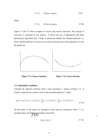
9. The objective function is, therefore
(7.23)
5.05.0
01.0)(
5.0
1
)( CCCCf +−=
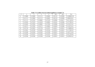
The sequence (Eq. 7.21) is used with δ = 0.01 and x0 = 0 and the results are shown in
Table 7-1. Since the value of the function increases until c = 5 and then decreases, i.e.,
f(0.31) > f(0.63) the optimum point has to lie in the range [0.31, 0.63]. It can be seen
that only seven iterations were needed to bracket the solution .To refine further the
interval another search can be carried out with a reduced value of δ starting with x0 =
0.31.
Table 7-1: Bracketing of the solution
k 0 1 2 3 4 5 6 7 8
C 0 0.01 0.03 0.07 0.15 0.31 0.63 1.27 2.55
f(C) 0 0.181 0.288 0.391 0.478 0.499 0.335 -0.274 -1.890
7.3.2 Optimization Methods Requiring Derivatives
In the previous section the necessary condition for the existence of an optimum was that
f '(x) = 0 (7.24)
This is a single variable (generally nonlinear) algebraic equation that can be solved
using any of the methods (Bisection, Newton-Raphson, Secant …) studied in chapter 3 .
If Newton-Raphson method is chosen then the iteration scheme is:
xn+1 = xn − f '(xn)/f ''(xn) (7.25)
The condition f(xn+1) > f(xn) (resp. f(xn+1) < f(xn)) should be checked for a maximum
(resp. minimum). Care should be taken for the selection of initial guess since this
sequence can fail near a turning point, i.e., f ''(xn) = 0 . It is also known, that unless the
function is unimodal, these methods will not necessarily find all the optimum points and
hence may converge on a local optimum.
9

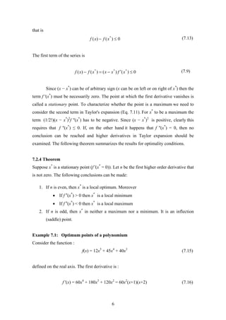
10. Example 7.3: Use of Newton method
The previous example 7.2 will be studied. The first and second derivative are readily
obtained
(7.26)
2
005.1
)(' −=
C
Cf
(7.27)CC
Cf
5025.0
)(''
−
=
Table 7-2 shows the iterations starting with the initial guess of C0 = 0.15 and converging
to the optimum value of C*
= 0.252506 with the maximum yield being f (C*) = 0.50501.
Table 7-2: Iterations to find optimum of Eq.(7.23) using Newton-Raphson method
Iteration Cn |f’(Cn)| |Cn−Cn-1|/|Cn-1|
0 0.150000E+00 0.594899E+00 -
1 0.218777E+00 0.148647E+00 0.458514E+00
2 0.249048E+00 0.138384E-01 0.138364E+00
3 0.252471E+00 0.141026E-03 0.137433E-01
4 0.252506E+00 0.149134E-07 0.141016E-03
7.3.3 Region-Elimination Methods
A number of search methods can be developed for the optimization of one-
single variable function, that do not use the derivative. Instead these search methods
locate the optimum by successively eliminating subintervals so as to reduce the interval
of search. These search methods are called region-elimination methods. In the following
one commonly used technique is presented.
7.3.3.1 Golden search method
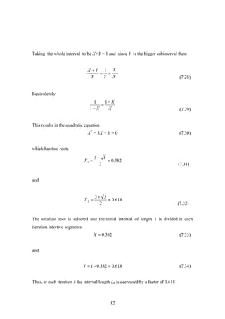
Consider, for example, the problem of finding a minimum for f(x) in the interval
[a,b]. Assume that f is unimodal and convex, hence, it has a global minimum.Consider
two arbitrary points x1 and x2 in the range [a,b]. Three cases are possible as far as the
values of f(x1) and f(x2) are concerned .In the first case (Figure 7.6a), we have f(x1) >
10

11. f(x2). A minimum can not be found in the region [a,x1] since this region contains values
for f such that f(x) > f(x1). This region can be eliminated from further consideration. In
the second case, (Figure 7.6b) we have f(x1) < f(x2). The region [x2,b] can not contain
the minimum and should be eliminated from consideration .The third case, (Figure
7-6c), f(x1) = f(x2) is not likely to occur because of round off errors. Therefore, if the
points x1 and x2 are suitably chosen a major portion of the interval can be eliminated in
each iteration .
Figure 7-6: Three possible cases for x1 and x2
Figure 7-7: Two lines segment for the Golden search method
In the golden search method the two points x1 and x2 are selected so that the
interval eliminated in one iteration will be of the same proportion to the total interval
regardless of the interval length.To achieve this, the ratio of the whole line to the larger
11

12. Taking the whole interval to be X+Y = 1 and since Y is the bigger subinterval then:
(7.28)X
Y
YY
YX
==
+ 1
Equivalently
(7.29)X
X
X
−
=
−
1
1
1
This results in the quadratic equation
X2
− 3X + 1 = 0 (7.30)
which has two roots
(7.31)
382.0
2
53
1 ≈
−
=X
and
(7.32)
618.0
2
53
2 ≈
+
=X
The smallest root is selected and the initial interval of length 1 is divided in each
iteration into two segments
382.0=X (7.33)
and
618.0382.01 =−=Y (7.34)
Thus, at each iteration k the interval length Lk is decreased by a factor of 0.618
12

13. Lk = 0.618 Lk-1 (7.35)
That is
Lk = (0.618)k
L0 (7.36)
where L0 is the length of the initial interval. This formula can be used to compute the
number of iterations required to reach a given precision. Let the desired final interval be
such that |Lk|≤ ε where ε is a given tolerance. Using (Eq. 7.36) the maximum number k
of iteration required to reach this accuracy is given by:
)0.618( k
L0 ≤ ε (7.37)
That is
(7.38)
618.0ln
)ln(
oL
k
ε
≥
Organigram 7.1: Golden Search Method
The algorithm for solving the one-dimensional minimization problem using the golden
search method is shown in Figure 7-8. For the maximization problem, the following
condition:
f(x1) > f(x2) (7.39)
should be replaced in the algorithm by:
f(x1) < f(x2) (7.40)
The stopping criteria are:
• The interval (L) is smaller than a given tolerance.
• The maximum number of iterations is exceeded.
13

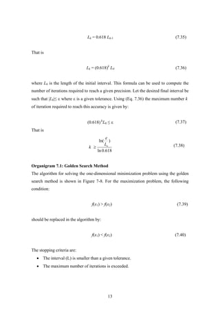
14. It should be noted also, that, for symmetric functions, the initial interval [a,b] should be
selected carefully, otherwise, the algorithm may not proceed since the following
condition:
f(x1) = f(x2) (7.41)
may occur.
Start
Input a,b,Kmax,
L = b - a
i > Kmax
f(x1) > f(x2)
b = x2
|x2-x1| <
a = x1
i = i +1
Stop
Yes
No
Yes
Print a,b,f(x1),f(x2)
Yes
No
No
bxax == 21 ,
Print maximum
iteration exceeded
Lbx
Lax
382.0
382.0
2
1
−=
+=
Figure 7-8: Golden search method for a minimization problem
14

15. Example 7.4: Golden search method
We reconsider the example 7.3 discussed earlier. The objective function is:
(7.43)
5.05.0
01.0)(
5.0
1
)( CCCCf +−=
where C∈[0.15,0.31]
At start (a,b) = (0.15,0.31) and L = 0.31 − 0.15 = 0.16. The two interior points are
x1 = a + Fs×L = 0.2111 (7.44)
x2 = b − Fs×L = 0.2489 (7.45)
Since f(x1) = 0.5013 < f(x2) = 0.5050 therefore in the next iteration a becomes x1 and b
remains unchanged. The interval of search becomes [0.2111, 0.3100]. The rest of
iterations are shown in Table 7-3. The optimum value up to a precision of 10-7
is x =
0.252506 corresponding to a yield of 0.50501.
7.4 OTHER SOLUTION TECHNIQUES
For the numerical solution of the necessary condition of optimization problem
i.e. f’(x) = 0, Newton-Raphson method has been covered. But the solution of this
nonlinear algebraic equation could also be carried out using bisection or secant method.
When the derivatives are difficult to obtain, they could be substituted by central finite
difference,
(7.46)
h
hxfhxf
xf
2
)()(
)('
−−+
≈
(7.47)
2
)()(2)(
)(''
h
hxfxfhxf
xf
−+−+
≈
A different class of techniques for the optimization of single variable consist in
approximating the function to be minimized in each iteration by a quadratic or cubic
polynomial interpolation. See references [31,39,49] for details.
15

16. 16
7.5 IMSL ROUTINES
Some IMSL routines to solve single variable optimization problems are as follows:
Routine Features
UVMIF
Find the minimum point of a smooth function of a single
variable using only function evaluations and using quadratic
interpolation method
UVMID
Find the minimum point of a smooth function of a single
variable using both function evaluations and first derivative
evaluations based on secant method or cubic interpolation

17. Table 7-3: Golden Search method applied to example 7.4
x f fK a b x1 2 (x1) (x2) |b-a|
0 0.150000 0.310000 0.211115 0.248885 0.501310 0.504986 0.160000E+00
1 0.211115 0.310000 0.211115 0.248885 0.501310 0.504986 0.988854E-01
2 0.211115 0.272229 0.248885 0.272229 0.504986 0.504271 0.611146E-01
3 0.234458 0.272229 0.234458 0.248885 0.504343 0.504986 0.377709E-01
4 0.234458 0.257802 0.248885 0.257802 0.504986 0.504958 0.233437E-01
5 0.243375 0.257802 0.243375 0.248885 0.504844 0.504986 0.144272E-01
10 0.251794 0.253095 0.251794 0.252291 0.505011 0.505012 0.130090E-02
15 0.252481 0.252598 0.252481 0.252526 0.505012 0.505012 0.117302E-03
20 0.252498 0.252509 0.252505 0.252509 0.505012 0.505012 0.105771E-04
25 0.252506 0.252507 0.252506 0.252507 0.505012 0.505012 0.953738E-06
30 0.252506 0.252506 0.252506 0.252506 0.505012 0.505012 0.859985E-07
17

18. 184