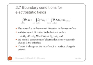
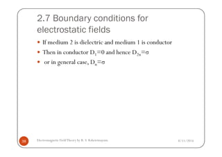
This document discusses electrostatics and related concepts. It begins by outlining what will be covered, including finding electrostatic fields for various charge distributions, the energy density of electrostatic fields, and how fields behave at media interfaces. It then defines Coulomb's law and the electric field, and discusses Gauss's law and how to use it to find electric fields from symmetric charge distributions. Finally, it covers electric potential, boundary value problems, and the electrostatic energy of charge distributions.
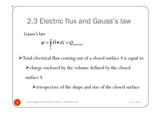
![2.3 Electric flux and Gauss’s law
( ) dvQdvDsdD
V
enclosed
VS
∫∫∫ ==•∇=•= ρψ
rvr
ψ
Since it is true for any arbitrary volume, we may equate the two
integrands and write,
Applying divergence theorem,
8/11/2014Electromagnetic FieldTheory by R. S. Kshetrimayum7
integrands and write,
Next we will discuss
How to find electric field from electric potential?
Easier since electric potential is a scalar quantity
0
= =D E
ρ
ρ
ε
∇ • ⇒ ∇ •
r r
[First law of Maxwell’s Equations]](https://image.slidesharecdn.com/2slides-150503000935-conversion-gate01/85/2-slides-7-320.jpg)
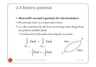
![2.4 Electric potential
1 2
+ 0
B A
A B
Path Path
E dl E dl∴ • • =∫ ∫
r rr r
∫ =•⇒ 0ldE
rr
8/11/2014Electromagnetic FieldTheory by R. S. Kshetrimayum12
Applying Stoke’s theorem, we have,
∫
( )∫ ∫ =•×∇=•⇒ 0sdEldE
rrrr
0=×∇ E
r [Second law of Maxwell’s
Equations for electrostatics]](https://image.slidesharecdn.com/2slides-150503000935-conversion-gate01/85/2-slides-12-320.jpg)