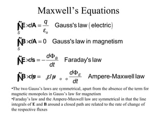
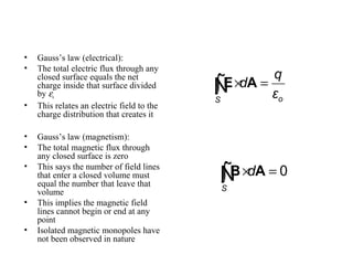
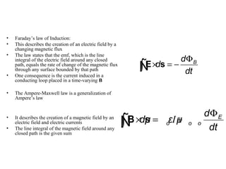
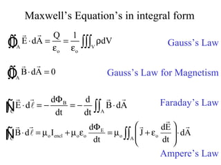
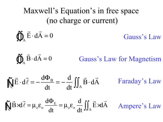
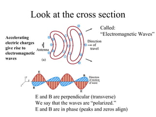
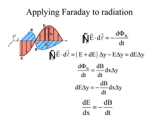
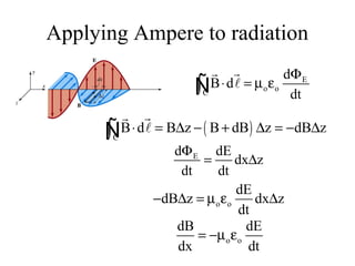
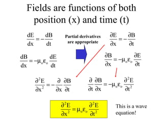
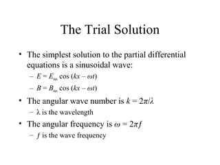
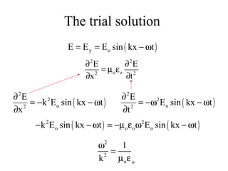
Maxwell's Equations describe the fundamental interactions between electric and magnetic fields. They consist of four equations: 1) Gauss's law relates electric charge density to electric field. 2) Gauss's law for magnetism states that magnetic monopoles have not been observed. 3) Faraday's law describes how a changing magnetic field induces an electric field. 4) Ampere-Maxwell law relates electric current and changing electric fields to magnetic fields. Together, Maxwell's Equations show that changing electric and magnetic fields propagate as electromagnetic waves moving at the speed of light.

1. Maxwell’s Equations
( )Gauss's law electric
0 Gauss's law in magnetism
Faraday's law
Ampere-Maxwell lawI
oS
S
B
E
o o o
q
d
ε
d
d
d
dt
d
dμ ε μ
dt
× =
× =
Φ
× = −
Φ
× = +
∫
∫
∫
∫
E A
B A
E s
B s
Ñ
Ñ
Ñ
Ñ
•The two Gauss’s laws are symmetrical, apart from the absence of the term for
magnetic monopoles in Gauss’s law for magnetism
•Faraday’s law and the Ampere-Maxwell law are symmetrical in that the line
integrals of E and B around a closed path are related to the rate of change of
the respective fluxes

2. • Gauss’s law (electrical):
• The total electric flux through any
closed surface equals the net
charge inside that surface divided
by εo
• This relates an electric field to the
charge distribution that creates it
• Gauss’s law (magnetism):
• The total magnetic flux through
any closed surface is zero
• This says the number of field lines
that enter a closed volume must
equal the number that leave that
volume
• This implies the magnetic field
lines cannot begin or end at any
point
• Isolated magnetic monopoles have
not been observed in nature
oS
q
d
ε
× =∫E AÑ
0
S
d× =∫B AÑ

3. • Faraday’s law of Induction:
• This describes the creation of an electric field by a
changing magnetic flux
• The law states that the emf, which is the line
integral of the electric field around any closed
path, equals the rate of change of the magnetic flux
through any surface bounded by that path
• One consequence is the current induced in a
conducting loop placed in a time-varying B
• The Ampere-Maxwell law is a generalization of
Ampere’s law
• It describes the creation of a magnetic field by an
electric field and electric currents
• The line integral of the magnetic field around any
closed path is the given sum
Bd
d
dt
Φ
× = −∫E sÑ
I E
o o o
d
dμ ε μ
dt
Φ
× = +∫B sÑ

4. Maxwell’s Equation’s in integral form
A V
o o
Q 1
E dA dV⋅ = = ρ
ε ε∫∫ ∫∫∫
rr
Ò
A
B dA 0⋅ =∫∫
rr
Ò
Gauss’s Law
Gauss’s Law for Magnetism
B
C A
d d
E d B dA
dt dt
Φ
⋅ = − = − ⋅∫ ∫∫
r rr r
lÑ
E
o encl o o o o
C A
d dE
B d I J dA
dt dt
 Φ
⋅ = µ + µ ε = µ + ε ⋅ 
 
∫ ∫∫
r
r rr r
lÑ
Faraday’s Law
Ampere’s Law

5. Maxwell’s Equation’s in free space
(no charge or current)
A
E dA 0⋅ =∫∫
rr
Ò
A
B dA 0⋅ =∫∫
rr
Ò
Gauss’s Law
Gauss’s Law for Magnetism
B
C A
d d
E d B dA
dt dt
Φ
⋅ = − = − ⋅∫ ∫∫
r rr r
lÑ
E
o o o oC A
d d
B d E dA
dt dt
Φ
× = µ ε = µ ε ×∫ ∫∫
r rr r
lÑ
Faraday’s Law
Ampere’s Law

6. Hertz’s Experiment
• An induction coil is connected to a
transmitter
• The transmitter consists of two spherical
electrodes separated by a narrow gap
• The discharge between the electrodes
exhibits an oscillatory behavior at a very
high frequency
• Sparks were induced across the gap of the
receiving electrodes when the frequency of
the receiver was adjusted to match that of
the transmitter
• In a series of other experiments, Hertz also
showed that the radiation generated by this
equipment exhibited wave properties
– Interference, diffraction, reflection,
refraction and polarization
• He also measured the speed of the radiation

7. Implication
• A magnetic field will be produced in empty space if there
is a changing electric field. (correction to Ampere)
• This magnetic field will be changing. (originally there
was none!)
• The changing magnetic field will produce an electric field.
(Faraday)
• This changes the electric field.
• This produces a new magnetic field.
• This is a change in the magnetic field.

8. An antenna
We have changed the magnetic
field near the antenna
Hook up an
AC source
An electric field results! This is
the start of a “radiation field.”

9. Look at the cross section
E and B are perpendicular (transverse)
We say that the waves are “polarized.”
E and B are in phase (peaks and zeros align)
Called:
“Electromagnetic Waves”
Accelerating
electric charges
give rise to
electromagnetic
waves

10. Angular Dependence of Intensity
• This shows the angular
dependence of the radiation
intensity produced by a dipole
antenna
• The intensity and power
radiated are a maximum in a
plane that is perpendicular to
the antenna and passing
through its midpoint
• The intensity varies as
(sin2
θ) / r2

11. Harmonic Plane Waves
x
At t = 0
At x = 0
λ
λ = spatial period or
wavelength
Τ
Τ = temporal period
2
v f
T T 2 k
λ π λ ω
= = λ = =
π
t
E
r
E
r

12. Applying Faraday to radiation
B
C
d
E d
dt
Φ
⋅ = −∫
rr
lÑ
( )C
E d E dE y E y dE y⋅ = + ∆ − ∆ = ∆∫
rr
lÑ
Bd dB
dx y
dt dt
Φ
= ∆
dB
dE y dx y
dt
∆ = − ∆
dE dB
dx dt
= −

13. Applying Ampere to radiation
E
o o
C
d
B d
dt
Φ
⋅ = µ ε∫
rr
lÑ
( )C
B d B z B dB z dB z⋅ = ∆ − + ∆ = − ∆∫
rr
lÑ
Ed dE
dx z
dt dt
Φ
= ∆
o o
dE
dB z dx z
dt
− ∆ = µ ε ∆
o o
dB dE
dx dt
= −µ ε

14. Fields are functions of both
position (x) and time (t)
o o
dB dE
dx dt
= −µ ε
dE dB
dx dt
= −
E B
x t
∂ ∂
= −
∂ ∂
o o
B E
x t
∂ ∂
= −µ ε
∂ ∂
2
2
E B
x x t
∂ ∂ ∂
= −
∂ ∂ ∂
2
o o 2
B E
t x t
∂ ∂ ∂
= −µ ε
∂ ∂ ∂
Partial derivatives
are appropriate
2 2
o o2 2
E E
x t
∂ ∂
= µ ε
∂ ∂
This is a wave
equation!

15. The Trial Solution
• The simplest solution to the partial differential
equations is a sinusoidal wave:
– E = Emax cos (kx – ωt)
– B = Bmax cos (kx – ωt)
• The angular wave number is k = 2π/λ
– λ is the wavelength
• The angular frequency is ω = 2πƒ
– ƒ is the wave frequency

16. The trial solution
( )y oE E E sin kx t= = − ω
2 2
o o2 2
E E
x t
∂ ∂
= µ ε
∂ ∂
( )
2
2
o2
E
E sin kx t
t
∂
= −ω − ω
∂
( )
2
2
o2
E
k E sin kx t
x
∂
= − − ω
∂
( ) ( )2 2
o o o ok E sin kx t E sin kx t− −ω = −µ ε ω − ω
2
2
o o
1
k
ω
=
µ ε

17. The speed of light
(or any other electromagnetic radiation)
o o
1
v c
k
ω
= = =
µ ε
2
v f
T T 2 k
λ π λ ω
= = λ = =
π

18. The electromagnetic spectrum
2
v f
T T 2 k
λ π λ ω
= = λ = =
π

20. Another look
dE dB
dx dt
= −
( )y oE E E sin kx t= = − ω
( ) ( )o o
d d
E sin kx t B sin kx t
dx dt
− ω = − − ω
( ) ( )o oE k cos kx t B cos kx t−ω = ω −ω
o
o o o
E 1
c
B k
ω
= = =
µ ε
( )z oB B B sin kx t= = − ω

21. Energy in Waves
2 2
0
0
1 1
u E B
2 2
= ε +
µ
o
o o o
E 1
c
B k
ω
= = =
µ ε
2
0u E= ε
2
0
1
u B=
µ
0
0
u EB
ε
=
µ

22. Poynting Vector
• Poynting vector points in the direction the wave moves
• Poynting vector gives the energy passing through a unit
area in 1 sec.
• Units are Watts/m2
( )
0
1
S E B= ×
µ
r r r
S cu=
r
= = =
2 2
o o o
E c BEB
S
μ μ c μ

23. Intensity
• The wave intensity, I, is the time average of
S (the Poynting vector) over one or more
cycles
• When the average is taken, the time average
of cos2
(kx - ωt) = ½ is involved
= = = = =
2 2
max max max max
av
2 2 2
I ave
o o o
E B E c B
S cu
μ μ c μ

24. Radiation Pressure
U
p
c
∆
∆ =
F 1 dp
P
A A dt
= =
aveS1 dU
P
Ac dt c
= =
r
Maxwell showed:
(Absorption of radiation
by an object)
What if the radiation reflects off an object?

25. Pressure and Momentum
• For a perfectly reflecting surface,
p = 2U/c and P = 2S/c
• For a surface with a reflectivity somewhere
between a perfect reflector and a perfect absorber,
the momentum delivered to the surface will be
somewhere in between U/c and 2U/c
• For direct sunlight, the radiation pressure is about
5 x 10-6
N/m2